2D Spin-Dependent Diffraction of Electrons From Periodical Chains of Nanomagnets

Abstract

The scattering of the unpolarized beams of electrons by nanomagnets in the vicinity of some scattering angles leads to complete spin polarized electrons. This result is obtained with the help of the perturbation theory. The dipole-dipole interaction between the magnetic moment of the nanomagnet and the magnetic moment of electron is treated as perturbation. This interaction is not spherically symmetric. Rather it depends on the electron spin variables. It in turn results in spinor character of the scattering amplitudes. Due to the smallness of the magnetic interactions, the scattering length of this process is very small to be proved experimentally. To enhance the relevant scattering lengths, we considered the diffraction of unpolarized beams of electrons by linear chains of nanomagnets. By tuning the distance between the scatterers it is possible to obtain the diffraction maximum of the scattered electrons at scattering angles which corresponds to complete spin polarization of electrons. It is shown that the total differential scattering length is proportional to N² (N is a number of scatterers). Even small number of nanomagnets in the chain helps to obtain experimentally visible enhancement of spin polarization of the scattered electrons.

1. Introduction

Modern technology enables to manufacture nanomagnets with anomalous magnetic moments [1,2,3]. Their physical properties have recently been studied experimentally, theoretically, and by computer simulation in [4,5,6,7,8,9]. The interaction between anomalous magnetic moment of the nanomagnet and the magnetic moment of electron manifests itself in the spin-dependent electron scattering. The spin-dependent scattering of electrons by nanomagnets in 2D geometry was studied for the first time theoretically in [10]. In this paper, in the Born approximation, we have studied the scattering of polarized beams of electrons by nanomagnets. The study indicated that such scattering can considerably change the polarization of the slow incident electrons. However, the scattering amplitudes of this process were relatively small due to the smallness of the magnetic interactions. The anisotropy of 2D spin-dependent electron scattering may be used to control the spin currents. The corresponding scattering amplitudes can be increased by using a large number of scatterers. The usage of periodical chains of nanomagnets with specially tuned distance between them allows one to use the diffraction properties of the scattering. This helps to obtain rather sharp maximums in the angle distribution of the polarized electrons.

In this paper, we consider the elastic 2D scattering of electron by nanomagnets. We find out that the probabilities of scattering depend on the spin polarization of incident and scattered electrons. With the help of the obtained scattering lengths, we consider the diffraction of the unpolarized beams of electrons from the linear periodical chains of nanomagnets and analyze the angular-spin dependence of the diffraction patterns.

2. Probabilities of Spin-Dependent Scattering by Nanomagnets

The Pauli equation of an electron moving in the magnetic field of the nanomagnet may be presented in the form

$$\widehat{H}=\frac{1}{2m}{\left[\widehat{p}+\frac{e}{c}\vec{A}\right]}^2+{\mu }_B\widehat{\sigma }·\vec{B}$$

(1)

Here m and e are the electron mass and its absolute charge respectively, p̂ is its momentum operator, A⃗ = µ⃗ × r⃗/r³, is the vector potential of the magnetic moment µ⃗, r⃗ is the radius vector, B⃗ = ▽⃗ × A⃗, ${\mu }_B=e\hslash /2mc$ is the Bohr magneton, and σ̂ are the Pauli matrices.

Below we consider the case when the magnetic moment of the nanomagnet µ⃗ is in the x − z plane.

For this case the Equation (1) is reduced to the 2D problem and takes the form

$$\widehat{H}=\frac{1}{2m}{\widehat{p}}_2^2+\widehat{V}\left(\vec{\rho }\right)$$

(2)

Here ${\widehat{p}}_2^2$ and ρ⃗ are the two dimensional momentum operator and the radius vector of the electron, respectively. The second term in Equation (2) describes the interaction between the magnetic moments of the electron and nanomagnet in the dipole-dipole approximation, which can be written as

$$\widehat{V}\left(\vec{\rho }\right)=\frac{{\mu }_B}{{\rho }^3}\left(3(\vec{\mu }·\vec{n})\vec{n}·\widehat{\sigma }-\vec{\mu }·\widehat{\sigma }\right)$$

(3)

where n⃗ is a unit vector along the radius vector ρ⃗.

Treating Equation (3) as a small perturbation, we use the Fermi golden rule and write down the probability of transition of the electron from the initial state i to the final state f as follows [11]

$$d{W}_{fi}=\left(\frac{2\pi }{\hslash }\right){\left|V_{f}i\right|}^2\delta (E_f-E_i)d{\nu }_f$$

(4)

where E_i and E_f are the energies of the electron in the initial and final state, respectively. V_fi is the matrix element of perturbation Equation (3), dν_f is the interval of the quantum numbers which corresponds to the final states.

Now we apply this formula to the transition from the state of the incident particle with momentum p⃗_i to the state with momentum p⃗_f. The interval of states dν_f can be written as d²p_f/(2πℏ)². First, we express the difference between energies in terms of their momenta

$$E_f-E_i=(p_f^2-p_i^2)/2m$$

(5)

Substituting Equation (5) into Equation (4) and using the property of delta function, we obtain

$$d{W}_{fi}=\left(\frac{m}{\pi {\hslash }^3}\right){\left|{\widehat{V}}_{fi}\right|}^2\delta (p_f^2-p_i^2)d^2{p}_f$$

(6)

.

The wave functions of the incident and the scattered electron are the products of the plane waves and spin wave functions

$$|i\rangle =\sqrt{\frac{m}{p}}\text{exp}\left(\frac{i{\vec{p}}_i·\vec{\rho }}{\hslash }\right)\vec{\chi }(S_i)$$

(7)

$$|f\rangle =\text{exp}\left(\frac{i\vec{p}{ }_f·\vec{\rho }}{\hslash }\right)\vec{\chi }(S_f)$$

(8)

The incident wave Equation (7) relates to the state with the momentum p⃗_i and S_i, and the scattered wave Equation (8) relates to p⃗_f and S_f, respectively. The incident wave function is normalized by the unit current density and the scattered wave function is normalized by the delta function [11].

With account of the above normalizations of the wave functions, the Equation (6) has dimension of length as it must be in 2D case and describes the differential scattering length. Integration in Equation (6) with respect to p_f with account of the relation dp²_f = 1/2d(p²_f)dφ gives the following expression of the differential scattering length

$$dL(k,\phi ;S_f,S_i)=\frac{m^2}{2\pi {\hslash }^{4}k}{\left|\langle \vec{\chi }(S_f)|{\displaystyle \int e^{-i\vec{q}·\vec{\rho }}\widehat{V}\left(\vec{\rho }\right)d^2\rho |\vec{\chi }(S_i)\rangle }\right|}^{2}d\phi$$

(9)

where q⃗ = k⃗ − k⃗₀, is the transferred momentum, k⃗₀ = p⃗_i/ℏ, k⃗ = p⃗_f/ℏ, $k_0^2=k^2=\frac{2mE}{{\hslash }^2}$, $q=2k\text{sin}\frac{\phi }{2},$ φ is the scattering angle. Integration in Equation (6) with account of the delta function means that we consider only elastic collisions.

Because of the spin-dependent character of the scattering, the differential scattering length Equation (9) includes the process with spin flipping and non-spin flipping. To distinguish them, it is better to use the spin-dependent scattering amplitudes introduced in [10]. Comparison of Equation (9) with corresponding result of [10] allows one to write down the following expression

$$dL(k,\phi ;S_f,S_i)={\left|\langle \vec{\chi }(S_f)|\vec{f}\left(k,\phi \right)\rangle \right|}^2$$

(10)

where the scattering amplitude f⃗(k, φ) is the two component spinor given by the relation

$$\vec{f}(k,\phi ) =-\frac{m}{{\hslash }^2\sqrt{2\pi k}}{\displaystyle \int e^{-i\vec{q}·\vec{\rho }\prime }\widehat{V}(\vec{\rho }\prime )\rho \prime d\rho \prime d\phi \prime |\vec{\chi }\left(S_i\right)\rangle }$$

(11)

It is worth noting that from Equation (10) one can not obtain the minus sign in Equation (11). It is obvious that the usage of the perturbation theory does not allow to obtain the phase factor [11]. The scattering amplitude Equation (11) was obtained in [10] with the help of the Born approximation. Its applicability coincides with the applicability of the perturbation theory |V̂| ≪ ℏ²/(mρ²), where ρ¯ is the range of action of the scattering potential V̂(ρ), which is given by Equation (3). For evaluation, we set $\left|V\right|\sim \frac{\mu \mu B}{{\rho }^3}$. Due to the fast decay of the magnetic dipole-dipole interaction with distance, we take ρ = 2a. Keeping this in mind, we obtain that the Born approximation is applicable if the following inequality is true [10]

$$\frac{16\pi \nu {\mu }_B^2{n}_{a}m{a}^2}{3{\hslash }^2}\ll 1$$

(12)

For the magnetic moment of nanoparticle, we used the formula $\mu =\frac{4\pi }{3}\nu {\mu }_B{n}_a{a}^3$, ν is a number of Bohr magnetons carried by the ferromagnetic atom, and n_a is the density of atoms of the nanomagnet. Substituting the numerical values of universal constants and n_a = 10²²cm⁻³ we obtain the following restriction on the size of the nanomagnet

$$a<\frac{100}{\sqrt{\nu }}nm$$

(13)

For the typical ν Equation (13) gives a of the order of 10 nm that allows us to consider only one domain nanomagnets.

The perturbation Equation (3) is non-spherically symmetric and depends on the spin degrees of freedom of the electron. This creates some problems while evaluating integral Equation (11). Basically the scattering amplitude is a two component spinor that depends on spin polarization of incident electron.

3. Scattering Amplitudes and Scattering Lengths

3.1. Magnetic Moment of Nanoparticle Parallel to the Velocity of Incident Electron

The scattering amplitude Equation (11) may be presented as

$$\vec{f}\left(k,\phi \right)=-\widehat{I}\vec{\chi }(S_i)$$

(14)

where the operator Î is given by

$$\widehat{I}=\frac{m}{{\hslash }^2\sqrt{2\pi k}}{\displaystyle \int e^{-i\vec{q}·\vec{\rho }\prime }\widehat{V}(\vec{\rho }\prime )d^2\rho \prime }$$

(15)

To evaluate integral Equation (15) one has to choose appropriate coordinate system. Figure 1 shows two coordinate systems. In the laboratory coordinate system (x, z), the magnetic moment of nanoparticle μ⃗ isalong the z-axis and the velocity of the incident electron is parallel to µ⃗. The calculation of Equation (15) is, however, convenient to carry out in other coordinate system (x′, z′) with x′-axis directed along q⃗, [10]. In this coordinate system, the dot product in the exponent Equation (15) has the simplest form q⃗ · ρ⃗′ = qρ′cosφ′ (ρ′ and φ′ are variables of integration), and Equation (15) can be written as

$$\begin{array}{l}\widehat{I}=\frac{m}{{\hslash }^2\sqrt{2\pi k}}{\displaystyle {\int }_0^{2\pi }{\displaystyle {\int }_{\alpha }^{\infty }{e}^{-iq\rho \prime \text{cos}\phi \prime }\widehat{V}(\vec{\rho }\prime )\rho \prime d\rho \prime d\phi \prime }}\end{array}$$

(16)

where a is the radius of the nanomagnet, and the operator of potential energy Equation (3) is given by

$$\widehat{V}=\frac{{\mu }_B}{\rho {\prime }^3}\left\{\left[{\mu }_{x\prime }\left(3{\text{cos}}^2\phi \prime -1\right)+\frac{3}{2}{\mu }_{z\prime }1\text{sin}2\phi \prime \right]{\widehat{\sigma }}_x+\left[{\mu }_{z\prime }（3{\text{sin}}^2\phi \prime -1｝+\frac{3}{2}{\mu }_{x\prime }\text{sin}2\phi \prime \right]{\widehat{\sigma }}_z\right\}$$

(17)

Figure 1. The coordinate systems: (x, z) and (x′, z′). The x′-axis is parallel to q⃗.

Figure 1. The coordinate systems: (x, z) and (x′, z′). The x′-axis is parallel to q⃗.

In the prime coordinate system, the magnetic moment µ has two com ${\mu }_{z\prime }=\mu \text{cos}\frac{\phi }{2}$, and ${\mu }_{x\prime }=-\mu \text{sin}\frac{\phi }{2}$. Inserting Equation (17) into Equation (16) and carrying out integration respect to φ′ we obtain

$$\widehat{I}\prime =\frac{6\pi \gamma }{a}\left(-I_1\sin \frac{\phi }{2}{\widehat{\sigma }}_x+I_2\cos \frac{\phi }{2}{\widehat{\sigma }}_z\right)$$

(18)

$$I_1=qa{\displaystyle {\int }_{qa}^{\infty }\frac{1}{x^2}\left[\frac{2}{3}{J}_0\left(x\right)-\frac{1}{x}{J}_1\left(x\right)\right]dx}$$

(19)

$$I_2=qa{\displaystyle {\int }_{qa}^{\infty }\frac{1}{x^2}\left[\frac{1}{x}{J}_1\left(x\right)-\frac{1}{3}{J}_0\left(x\right)\right]dx}$$

(20)

where $\gamma =-\frac{m\mu {\mu }_B}{{\hslash }^2\sqrt{2\pi k}}$, J₀(x), and J₁(x) are the first kind Bessel functions of the zeroth, and first order, respectively. Details of calculations of the integrals I₁ and I₂ are given in Appendixes (A1 − A8). In Equations (19) and (20), we introduced new variable of integration x = qρ′. It is necessary to remember that result Equation (18) is obtained in the x′ – z′ coordinate system.

To get the correct expression of the scattering amplitudes in the laboratory coordinate system, we can proceed in the following way: transform the spinor χ⃗(S_i) to x′ – z′ coordinate system, find the result Î′χ⃗(S_i), and transform this result back to the laboratory coordinate system.

Let us consider the unpolarized beam of electrons, which is in the x − z coordinate given by the linear combination of the spinors

$$\vec{\chi }(S_i)=\alpha \left|\begin{array}{c}1\\ 0\end{array}\right|+\beta \left|\begin{array}{c}0\\ 1\end{array}\right|$$

(21)

with α² + β² = 1, α² is the fraction of electrons whose spin is parallel to their initial velocity (along z-axis) and β² is the fraction of electrons with opposite spin. By carrying out the above specified operations, we obtain

$$\vec{f}\left(\phi \right)=f_{\uparrow }^{\left|\right|}\left(\phi \right)\left(\begin{array}{c}1\\ 0\end{array}\right)+f_{\downarrow }^{\left|\right|}\left(\phi \right)\left(\begin{array}{c}0\\ 1\end{array}\right)$$

(22)

where

$$f_{\uparrow }^{\left|\right|}\left(\phi \right)=\frac{6\gamma \pi }{a}\left[\alpha \left(I_1{\sin }^2\frac{\phi }{2}+I_2{\cos }^2\frac{\phi }{2}\right)+\frac{\beta }{2}\left(I_2-I_1\right)\sin \phi \right]$$

(23)

$$f_{\downarrow }^{\left|\right|}\left(\phi \right)=\frac{6\gamma \pi }{a}\left[-\beta \left(I_1{\sin }^2\frac{\phi }{2}+I_2{\cos }^2\frac{\phi }{2}\right)+\frac{\alpha }{2}\left(I_2-I_1\right)\sin \phi \right]$$

(24)

The quantity $f_{\uparrow }^{\left|\right|}\left(\phi \right)$ and $f_{\downarrow }^{\left|\right|}\left(\phi \right)$ are the scattering amplitudes of electrons having spin up and down after scattering, respectively. The denotation I stands for the initial electron velocity, which is parallel to the magnetic moment of the nanomagnet. It would be convenient to present Equations (23) and (24) as

$$f_{\uparrow }^{\left|\right|}\left(ka,\phi \right)=\sqrt{L_0}\left[\alpha \sqrt{{\tilde{L}}_1}+\beta \sqrt{{\tilde{L}}_3}\right]$$

(25)

$$f_{\downarrow }^{\left|\right|}\left(ka,\phi \right)=\sqrt{L_0}\left[-\beta \sqrt{{\tilde{L}}_1}+\alpha \sqrt{{\tilde{L}}_3}\right]$$

(26)

Here we introduced the quantity with dimension of length

$$L_0=32{\pi }^3{a}^5{\nu }^2{\left(\frac{{\mu }_B^2{n}_{a}m}{{\hslash }^2}\right)}^2$$

(27)

and the dimensionless parameters

$${\tilde{L}}_1=\frac{1}{ka}{\left[I_1{\sin }^2\frac{\phi }{2}+I_2{\cos }^2\frac{\phi }{2}\right]}^2$$

(28)

$${\tilde{L}}_3=\frac{1}{4ka}{\left[I_2-I_1\right]}^2{\sin }^2\phi$$

(29)

We also express the magnetic moment of nanomagnet as $\mu =\frac{4\pi }{3}\nu {\mu }_B{a}^3{n}_a$ (n_a is a density number of atoms in nanomagnets, ν is a number of Bohr magnetons per atom of the nanomagnet). The differential scattering lengths for the specified processes are given by

$${\left|f_{\uparrow }^{\left|\right|}\left(ka,\phi \right)\right|}^2= L_0{\left[\alpha \sqrt{{\tilde{L}}_1}+\beta \sqrt{{\tilde{L}}_3}\right]}^2$$

(30)

$${\left|f_{\downarrow }^{\left|\right|}\left(ka,\phi \right)\right|}^2=L_0{\left[-\beta \sqrt{{\tilde{L}}_1}+\alpha \sqrt{{\tilde{L}}_3}\right]}^2$$

(31)

In [10], we considered the scattering amplitudes of the polarized beam of electrons. These results can be recovered from Equations (30) and (31) setting α = 1, β = 0 and α = 0, β = 1.

3.2. Magnetic Moment of Nanomagnet Perpendicular to Velocity of Incident Electron

Now we consider the case when the magnetic moment µ⃗ is transverse to z-axis and the velocity v⃗ of electrons along the z-axis. Let µ⃗ be along positive x-axis. Acting as in the pervious subsection and taking in to account that the components of the magnetic moment of the nanomagnet in Equation (17) are ${\mu }_{x\prime }=\mu \cos \frac{\phi }{2}$ and ${\mu }_{z\prime }=\sin \frac{\phi }{2}$, we obtain the following scattering amplitudes

$$\vec{f}\left(\phi \right)=f_{\uparrow }^{\perp }(\phi )\left(\begin{array}{c}1\\ 0\end{array}\right)+f_{\downarrow }^{\perp }(\phi )\left(\begin{array}{c}0\\ 1\end{array}\right)$$

(32)

where $f_{\uparrow }^{\perp }(\phi )$ and $f_{\downarrow }^{\perp }(\phi )$ represent the spin-dependent 2D scattering amplitudes of electron with initial velocity perpendicular (⊥) to µ⃗ with the spin up and down after scattering, respectively. The scattering amplitudes $f_{\uparrow }^{\perp }(\phi )$ and $f_{\downarrow }^{\perp }(\phi )$ may be presented as

$$f_{\uparrow }^{\perp }(\phi )=\sqrt{L_0}\left[\beta \sqrt{{\tilde{L}}_2}+\alpha \sqrt{{\tilde{L}}_3}\right]$$

(33)

$$f_{\downarrow }^{\perp }(\phi )=\sqrt{L_0}\left[\alpha \sqrt{{\tilde{L}}_2}-\beta \sqrt{{\tilde{L}}_3}\right]$$

(34)

where we used Equations (27) and (29) together with

$${\tilde{L}}_2=\frac{1}{ka}{\left[I_1{\cos }^2\frac{\phi }{2}+I_2{\sin }^2\frac{\phi }{2}\right]}^2$$

(35)

The differential scattering lengths can be presented as

$${\left|f_{\uparrow }^{\perp }(ka,\phi )\right|}^2=L_0{\left[\beta \sqrt{{\tilde{L}}_2}+\alpha \sqrt{{\tilde{L}}_3}\right]}^2$$

(36)

$${\left|f_{\downarrow }^{\perp }(ka,\phi )\right|}^2=L_0{\left[\alpha \sqrt{{\tilde{L}}_2}-\beta \sqrt{{\tilde{L}}_3}\right]}^2$$

(37)

The next section discusses the general properties of the differential scattering lengths (30, 31) and (36, 37) as functions of the scattering angle φ and the dimensionless parameter ka, which characterizes the energy of unpolarized beams of incident electrons $\alpha =\beta =1/\sqrt{2}$.

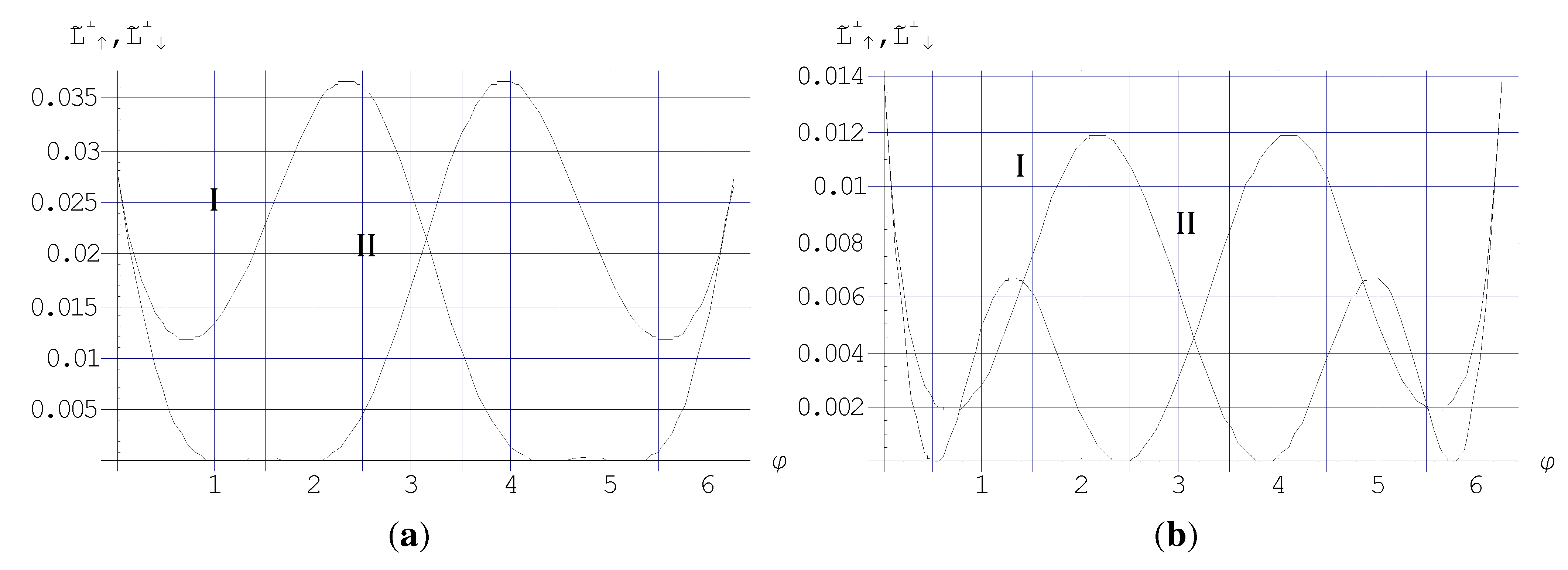
4. Graphical Presentations of the Scattering Lengths of Unpolarized Beams of Electrons by Nanomagnets

The above formulas help us to specify peculiarities of scattering of unpolarized beams of electrons. Consider the scattering of electrons initially moving parallel to µ⃗ (Equations (30) and (31)) and perpendicular to µ⃗(Equations (36) and (37)). Thus, we present the graphs of the following dimensionless differential scattering lengths

$${\tilde{L}}_{\uparrow }^{\left|\right|}=\frac{1}{L_0}\frac{d{L}_{\uparrow }^{\left|\right|}}{d\phi }=\frac{1}{L_0}{\left[f_{\uparrow }^{\left|\right|}(ka,\phi )\right]}^2$$

(38)

$${\tilde{L}}_{\downarrow }^{\left|\right|}=\frac{1}{L_0}\frac{d{L}_{\downarrow }^{\left|\right|}}{d\phi }=\frac{1}{L_0}{\left[f_{\downarrow }^{\left|\right|}(ka,\phi )\right]}^2$$

(39)

$${\tilde{L}}_{\uparrow }^{\perp }=\frac{1}{L_0}\frac{d{L}_{\uparrow }^{\perp }}{d\phi }=\frac{1}{L_0}{\left[f_{\uparrow }^{\perp }(ka,\phi )\right]}^2$$

(40)

$${\tilde{L}}_{\downarrow }^{\perp }=\frac{1}{L_0}\frac{d{L}_{\downarrow }^{\perp }}{d\phi }=\frac{1}{L_0}{\left[f_{\downarrow }^{\perp }(ka,\phi )\right]}^2$$

(41)

In [10], we obtained that 2D spin-dependent scattering of polarized beams of electrons by nanomagnets is practically isotropic for very slow particles ka ≪ 1. It is true for the scattering of unpolarized beams of slow electrons as well. Let us consider the scattering of electrons with the initial velocity v⃗ parallel to µ⃗.

Figure 2(a) shows the scattering lengths for spin up (curve I) and spin down (curve II). The maximum difference between these scattering lengths is 8% for φ = 2 rad. It allows us to claim that the scattering is anisotropically weak. With increasing in ka, the scattering becomes anisotropic. The ratio of numbers of the scattered electrons with spin up and spin down depends on φ. Figure 2(b) illustrates the scattering lengths for ka = 0.2. At φ ≃ π/2, the ratio of ${\tilde{L}}_{\uparrow }^{\left|\right|}$ to ${\tilde{L}}_{\downarrow }^{\left|\right|}$ is about 4. This is to mean that around the scattering angle φ = π/2 rad, about 80% of the scattered electrons have spin up and 20% spin down. However, the values of the corresponding scattering lengths are very small and become smaller with further increase in ka.

Figure 2. ${\tilde{L}}_{\uparrow }^{\left|\right|}$ (curve I) and ${\tilde{L}}_{\downarrow }^{\left|\right|}$ (curve II) versus φ (in radian). (a) for ka = 0.01, and (b) for ka = 0.2 according to Equations (38) and (39).

Figure 2. ${\tilde{L}}_{\uparrow }^{\left|\right|}$ (curve I) and ${\tilde{L}}_{\downarrow }^{\left|\right|}$ (curve II) versus φ (in radian). (a) for ka = 0.01, and (b) for ka = 0.2 according to Equations (38) and (39).

Figure 3(a) and 3(b) illustrates the scattering of unpolarized beams of electron by nanomagnets for ka = 0.5 and ka = 1, respectively. As one can see, the scattering lengths become smaller as the energy of the incident electron increases. The polarization of the beams considerably increases, and for particular values of φ one can get almost complete polarization. Figure 3(a) reveals that around φ = π/2 rad practically all scattered electrons have spin up and around φ = 3π/2 rad they have spin down. The complete polarization can also be seen in Figure 3(b) at φ = 1 and φ = 4 rad (spin up) and at φ = 2.3 and φ = 5.3 rad (spin down). The inspections of Figure 3(a) and 3(b) shows that in the range 0.5 < ka < 1, the scattering length roughly behaves like 1/ka.

Figure 3. ${\tilde{L}}_{\uparrow }^{\left|\right|}$ (curve I) and ${\tilde{L}}_{\downarrow }^{\left|\right|}$ (curve II) versus φ(in radian). (a) for ka = 0.5, and (b) for ka = 1 according to Equations (38) and (39).

Figure 3. ${\tilde{L}}_{\uparrow }^{\left|\right|}$ (curve I) and ${\tilde{L}}_{\downarrow }^{\left|\right|}$ (curve II) versus φ(in radian). (a) for ka = 0.5, and (b) for ka = 1 according to Equations (38) and (39).

Let us consider the scattering of unpolarized beams of electrons with initial velocity perpendicular to µ⃗. Figure 4(a) and Figure 4(b) presents the corresponding scattering lengths of electrons for ka = 0.01 and ka = 0.2, respectively. The properties of this scattering are practically the same compared to the above described Figure 2. Particularly, for ka = 0.01, the scattering is anisotropically weak, and for ka = 0.2, ratio of the scattering lengths for electrons with spin up and spin down around φ = π/2 rad is close to 4, just as the case of µ⃗ parallel to v⃗.

Figure 4. ${\tilde{L}}_{\uparrow }^{\perp }$ (curve I) and ${\tilde{L}}_{\downarrow }^{\perp }$ (curve II) versus φ (in radian). (a) for ka = 0.01, and (b) for ka = 0.2 according to Equations (40) and (41).

Figure 4. ${\tilde{L}}_{\uparrow }^{\perp }$ (curve I) and ${\tilde{L}}_{\downarrow }^{\perp }$ (curve II) versus φ (in radian). (a) for ka = 0.01, and (b) for ka = 0.2 according to Equations (40) and (41).

Figure 5(a) and Figure 5(b) indicates the scattering lengths ${\tilde{L}}_{\uparrow }^{\perp }$ (curve I) and ${\tilde{L}}_{\downarrow }^{\perp }$ (curve II) versus φ, respectively. Just as the case of µ⃗ parallel to v⃗, we have complete polarization of the electron beams for particular values of φ. For example, for ka = 0.5 around φ = 1 and 2 rad practically all electrons have spin up and around φ = 4.3 and 5.3 rad almost all electrons have spin down.

Figure 5. ${\tilde{L}}_{\uparrow }^{\perp }$ (curve I) and ${\tilde{L}}_{\downarrow }^{\perp }$ (curve II) versus φ (in radian). (a) for ka = 0.5, and (b) for ka = 1 according to Equations (40) and (41).

Figure 5. ${\tilde{L}}_{\uparrow }^{\perp }$ (curve I) and ${\tilde{L}}_{\downarrow }^{\perp }$ (curve II) versus φ (in radian). (a) for ka = 0.5, and (b) for ka = 1 according to Equations (40) and (41).

Figure 5(b) shows that around φ = 0.5 and 2.5 rad practically all spins of electrons pointed up and for φ = 3.8 and 5.8 rad their spins are down. The dimensionless differential scattering lengths behave like 1/ka in the range of 0.5 ≤ ka ≤ 1.

From the above graphs it is possible to conclude that at particular scattering angles in the range of 0.5 ≤ ka ≤ 1, the initially unpolarized beam of electrons becomes practically completely polarized. However, the corresponding scattering lengths are relatively small. The scattering lengthes can considerably increase through interference effects of periodical structures of nanomagnets.

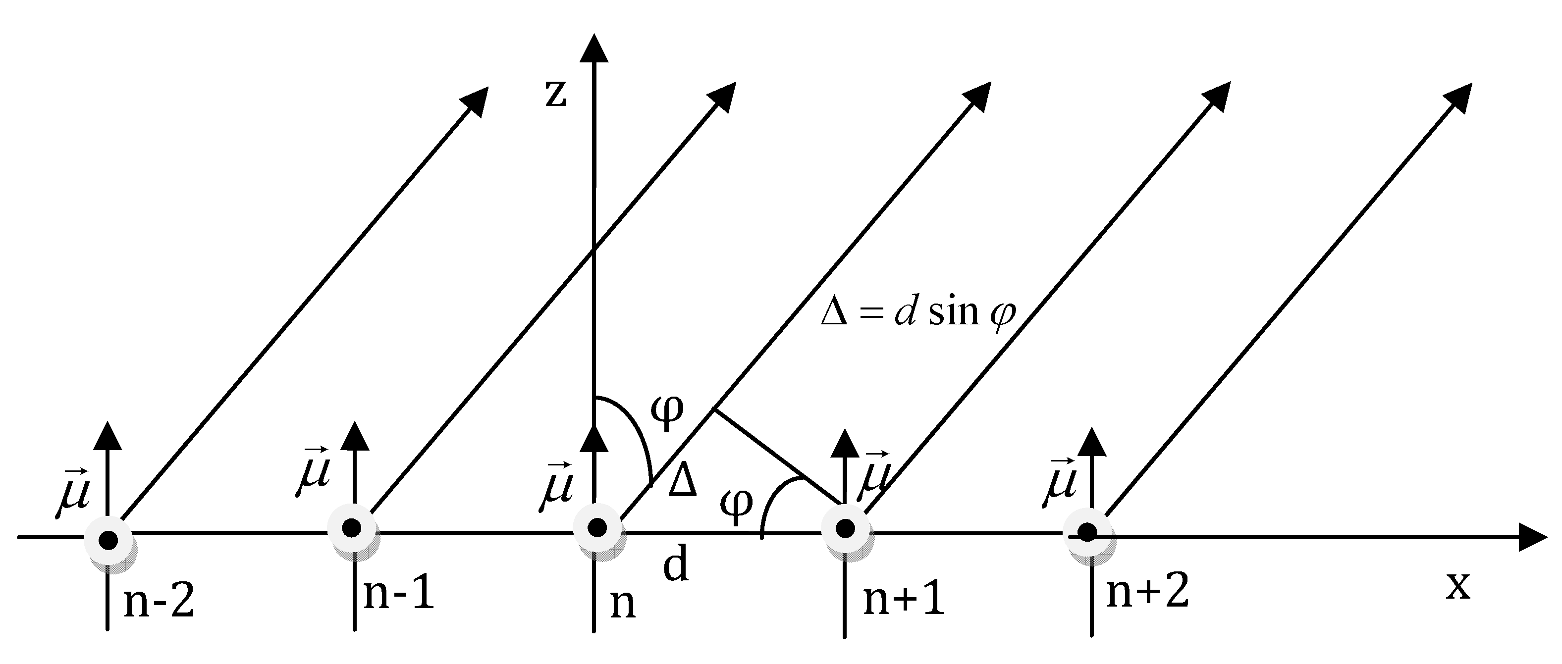
5. Diffraction of Electrons by Linear Chains of Nanomagnets

Consider the scattering of electrons from a linear chain of equally spaced nanomagnets with lattice constant d. We assume that all nanomagnets are identical. The magnetic moments of the nanomagnets are directed along the z-axis (see Figure 6). This linear chain of nanomagnets can be treated as a diffraction grating for 2D electron beams. According to the Huygens–Fresnel principle, every individual nanomagnet can be treated as the source of the cylindrical waves. In the case of 2D spin-dependent scattering by nanomagnets, the amplitude of the scattered wave depends on the scattering angle. As it was illustrated in the previous section, there are some scattering angles (for particular energy of incident electrons) where the unpolarized incident beams of electrons is practically completely polarized. Particularly, according to Figure 3(a), the scattered particles with ka = 0.5 are completely polarized at φ = 1.5 rad. Similarly, it follows from Figure 3(b) that complete polarization is observed for scattered electrons with ka = 1 at φ = 1 rad.

Figure 6. Scattering of electrons by linear chains of nanomagnets.

Figure 6. Scattering of electrons by linear chains of nanomagnets.

Consider the case when all path differences ∆ (∆ = d sinφ) between the neighboring scattered beams are the same. This condition allows us to find the distance between nanomagnets when all the scattering amplitudes added coherently (if they put together by focusing the electrons beams far from the chain of the nanomagnets). This condition gives the following relation for the distance between the nanomagnets

$$d=\frac{2\pi a}{ka\sin {\phi }_d}$$

(42)

where a is the radius of individual nanomagnets and φ_d is the scattering angle corresponding to almost the complete polarization. Let us apply this relation to the case ka = 0.5 and φ_d = 1.5 rad = 87°. Substituting this parameters in Equation (42), we get d = 4πa ≫ a. The last condition is favorable for not taking into account the multiple scattering by the neighboring nanomagnets. The typical size of the nanomagnet a must satisfy inequality Equation (13). For large nanomagnets, the magnetization vectors of the scatterers in the chain will wander and destroy constructive interference.

It is clear that the resultant scattering amplitude at the scattering angle φ_d is proportional to N (N is the number of the scatterers). The total scattering length corresponding to N scatterers is ~ N²${\tilde{L}}_{\uparrow }^{\left|\right|}$ ≃ 2.5 × 10⁻²N². Even setting N = 10, we get considerable increment in the scattering lengths.

We considered the chain of scatterers with magnetic moment parallel to z-axis (Figure 6). In the same manner, one can consider the chain of nanomagnets with the magnetic moments transverse to z-axis. In this case, the largest scattering length of complete polarization ${\tilde{L}}_{\uparrow }^{\perp }$ ≃ 0.034 is obtained for ka = 0.5 at φ = 2 rad (Figure 5(a)). It is similar to the chain with µ⃗ parallel to z-axis. However, it is necessary to note that the scattering angle φ = 2 rad relates to the back scattering that may complicate the experimental verification of the theory.

Conclusions

In this paper, we consider 2D scattering of unpolarized beams of electrons by nanomagnets. Treating the interaction between the magnetic moments of the nanomagnet and the electron as a small perturbation, we obtained the scattering amplitudes and scattering lengths.

One of the main finding of this work is that at particular scattering angles it is possible to obtain practically all scattered electrons with the same orientation of their spin. However, the corresponding scattering lengths are relatively small. To increase these scattering lengths, we propose to use the diffraction of unpolarized electron beams from the periodical chains of nanomagnets. We studied the diffraction of electrons by a linear periodic chain of nanomagnets. In the case of convectional diffraction, any scatterer is considered as a source of spherical wave with the amplitude which does not depend on the scattering angle. The scattering potential is not spherically symmetric. Moreover, it depends on the spin variables of the electron. This results in strong angular anisotropy of the scattering and its dependence on the spin orientation of electrons at the specified energy range of incident electrons.

By tuning the distance between the nanomagnets, it is possible to organize a diffraction maximum at the scattering angles which correspond to the dominant spin polarization of the scattered electrons. The study concluded that the resultant differential scattering length is proportional to N², which is typical for diffraction processes. Even for N = 10, the enhancement of the scattering lengths due to diffraction will be of the order of 10².

References

1. Nieuwenhuys, G.J. Magnetic behavior of cobalt, iron, and manganese dissolved in palladium. Adv. Phys. 1975, 24, 515–519. [Google Scholar] [CrossRef]
2. Hong, N.H.; Sakai, J.; Prellier, W.; Hassini, A. Transport Cr-doped SnO2 thin films: Ferromagnetism beyoned room temperature with a giant magnetic moment. J. Phys. Condens. Matter 2005, 17, 1697–1702. [Google Scholar] [CrossRef]
3. Kabir, M.; Kanhere, D.G.; Mookerjee, A. Large magnetic moments and anomalous exchange coupling in As-doped Mn clusters. Phys. Rev. B 2006, 73, 075210:1–075210:4. [Google Scholar]
4. Liu, L.; Guo, G.Y.; Jayanthi, C.S.; Wu, S.Y. Colossal Paramagnetic moments in metallic carbon nanotori. Phys. Rev. Lett. 2002, 88, 217206:1–217206:4. [Google Scholar]
5. Ogale, S.B.; Chouldhary, R.J.; Buban, J.P.; Lofland, S.E.; Shinde, S.R.; Kale, S.N.; Kulkarni, V.N.; Higgins, J.; Lanci, C.; Simpson, J.R.; Browning, N.D.; Sarma, S.D.; Drew, H.D.; Green, R.L.; Venkatesan, T. High temperature ferromagnetism with a giant magnetic moment in transport Co-doped SnO2δ. Phys. Rev. Lett. 2003, 91, 077205:1–077205:4. [Google Scholar] [CrossRef]
6. Jung, M.-H.; Lee, S.-I. Giant magnetic moment of oxygen-free CuNi nanoparticles. J. Nanosci. Nanotechnol. 2009, 9, 3201–3203. [Google Scholar] [CrossRef] [PubMed]
7. Ito, Y.; Miyazaki, A.; Takai, K.; Sivamurugan, V.; Maeno, T.; Kadono, T.; Kitano, M.; Ogawa, Y.; Nakamura, N.; Hara, M.; Valiyaveetti, S.; Enoki, T. Magnetic sponge prepared with an alkanedithiol-bridged network of nanomagnets. J. Am. Chem. Soc. 2011, 133, 11470–11473. [Google Scholar] [CrossRef] [PubMed]
8. Wang, J.; Beeli, P.; Ren, Y.; Zhao, G.-M. Giant magnetic moment enhancement of nickel nanopar- ticles embedded in multiwalled carbon nanotubes. Phys. Rev. B. 2010, 82, 193410:1–193410:4. [Google Scholar]
9. Qun, J.J.; Cao, H.-B.; Ge, G.-X.; Wang, Y.X.; Yan, H.-X.; Zhang, Z.-Y.; Liu, Y.-H. Giant magnetic moment of the core-shell Co13@Mn20 clusters: First principles calculation. J. Comb. Chem. 2011, 32, 2474–2478. [Google Scholar] [CrossRef]
10. Mal’nev, V.N.; Senbeta, T. Spin-dependent 2D electron scattering by Nanomagnets. J. Magnet. Magnet. Mater. 2011, 323, 1581–1587. [Google Scholar] [CrossRef]
11. Landau, L.D.; Lifshitz, E.M. Quantum Mechanics: Non-Relativistic Theory, 3rd ed.; Pergamon Press: Oxford, UK, 1977. [Google Scholar]
12. Taylor, J.R. Scattering Theory: The Quantum Theory of Nonrelativistic Collisions; Dover Publications,Inc.: Mineola, NY, USA, 2000. [Google Scholar]