Article

Using GM (1,1) Optimized by MFO with Rolling Mechanism to Forecast the Electricity Consumption of Inner Mongolia

School of Economics and Management, North China Electric Power University, Beijing 102206, China
*
Author to whom correspondence should be addressed.
Appl. Sci. 2016, 6(1), 20; https://doi.org/10.3390/app6010020
Submission received: 21 November 2015 / Revised: 27 December 2015 / Accepted: 8 January 2016 / Published: 15 January 2016

Abstract

:
Accurate and reliable forecasting on annual electricity consumption will be valuable for social projectors and power grid operators. With the acceleration of electricity market reformation and the development of smart grid and the energy Internet, the modern electric power system is becoming increasingly complex in terms of structure and function. Therefore, electricity consumption forecasting has become a more difficult and challenging task. In this paper, a new hybrid electricity consumption forecasting method, namely grey model (1,1) (GM (1,1)), optimized by moth-flame optimization (MFO) algorithm with rolling mechanism (Rolling-MFO-GM (1,1)), was put forward. The parameters a and b of GM (1,1) were optimized by employing moth-flame optimization algorithm (MFO), which is the latest natured-inspired meta-heuristic algorithm proposed in 2015. Furthermore, the rolling mechanism was also introduced to improve the precision of prediction. The Inner Mongolia case discussion shows the superiority of proposed Rolling-MFO-GM (1,1) for annual electricity consumption prediction when compared with least square regression (LSR), GM (1,1), FOA (fruit fly optimization)-GM (1,1), MFO-GM (1,1), Rolling-LSR, Rolling-GM (1,1) and Rolling-FOA-GM (1,1). The grey forecasting model optimized by MFO with rolling mechanism can improve the forecasting performance of annual electricity consumption significantly.

Graphical Abstract

1. Introduction

Electricity consumption is one of the significant indices of electrical power supply system planning and operation management. The characteristics analysis of electric power consumption is the primary requirement for the quality, stable, economic and safe operation of power grid. Since it is very difficult to store electric energy, precise and reliable forecasting on electricity consumption is of great significance to satisfy the continuously increasing demand for electricity, sustain the industrialization development, and formulate long-term stable energy policy [1].
Since the 1970s, much literature has focused on developing various kinds of forecasting techniques for electric energy [2]. The traditional forecasting methods mainly include electric elasticity coefficient method [3], trend extrapolation technique [4], regression analysis method [5,6,7], time series method [8], and so on. However, the traditional approach greatly depends on an accurate model. Some parameters are set as fixed values in the process of prediction so that the forecasting results would be difficult for reflecting the real electricity demand accurately, which causes the traditional models to show a poor performance for electricity consumption forecasting in terms of accuracy and reliability [9].
With the acceleration of electricity market reformation and the development of smart grid and the energy Internet, the modern power grid is becoming increasingly complex in terms of structure and function. Simultaneously, with the continuous progress of modern science and technology and the gradual deepening of basic theory research, the emergence of interdisciplinary theory provides a solid theoretical and mathematical foundation for the accurate prediction of electric energy demand. Metaxiotis et al. [10] stated that the artificial intelligence algorithms have been widely applied in various fields, mostly due to their symbolic reasoning, flexibility and explanation capabilities. Wang and Yang [11] proposed a prediction model in terms of non-linear combined neural network, which can effectively take account of the merits of non-linear regression analysis and artificial neural network. Azadeh et al. [12] used time, temperature, and historical loads as inputs of an artificial neural networks (ANN) model for a more accurate short-term forecasting, and ANN-based results are compared to that of conventional regression models. It is observed that ANN models are superior to regression models in most cases in accordance with mean absolute percentage error (MAPE). Ma et al. [13] presented a new power load forecasting method on the basis of fuzzy inference and ANN, and a practical example was used to show that the prediction accuracy could be enhanced using the proposed method. Chen and Wang [14,15] presented a collaborative fuzzy-neural approach based on fuzzy back propagation networks to predict annual electricity consumption. AlRashidi and EL-Naggar [16] presents a particle swarm optimization (PSO) as an innovation to forecast annual peak load for Kuwait and Egypt. Cong et al. [17] used three kinds of kernel functions (radial basis kernel functionlinear, and poly) to establish a prediction model based on support vector machine (SVM) theory, and the fitting degree was tested with three evaluating indicators, namely MAPE, PMSE and Theil IC. Cheng and Chen [18] combined BP, GM (1,1), triple exponential smoothing model, and polynomial trend extrapolation model together to accurately forecast energy consumption. Xue and Cao [19] established a combination forecasting model consisting of neural network, grey forecasting model and time series model to predict Chinese energy consumption. Because the selection of the parameters of some intelligent algorithms and the weight coefficients of the combination forecasting models exerted a great influence on the prediction accuracy, many scholars have performed a number of researches related to the method of parameter selection and optimization. Liang [20] raised a prediction model based on the improved fruit fly algorithm to optimize the parameters of SVM so that the accuracy of forecasting can be enhanced. Li et al. [21] used a modified PSO combined with simulated annealing algorithm (SA) to optimize SVM. Wu et al. [22] used genetic algorithms to obtain the best-optimized parameter values of SVM model to enhance the precision of forecasting. Wang et al. [23] used support vector regression optimized by differential evolution algorithm to predict electricity consumption. Zhao et al. [24] employed fruit fly optimization algorithm to obtain the weights of combination forecasting model for urban saturated power load analysis.
The grey system theory proposed by Chinese professor Deng Julong is a theory that deals with uncertainty issues with the characteristics of less data and imperfect information [25]. Grey model (1,1) (GM (1,1)), which is a kind of grey forecasting model, has been employed in many forecasting problems, such as the prediction of short term and long term electric load [26,27], tourism flow [28], airline industry [29], automobile production [30], wave [31], wind speed and wind power [32], per capita annual net income forecast of rural households [33], fuel production [34], and carbon emissions, energy demand and economic growth [35]. Since the power system also has the characteristics of grey system, GM (1,1) has been used in electric energy demand forecasting [36,37,38,39]. However, the accuracy of electricity demand prediction is affected by many factors, such as political environment, economic development and social status. Therefore, the exponentially growing rule of GM (1,1) may not show a good forecasting performance in electricity demand prediction. Under this circumstance, the optimization of GM (1,1) is widely discussed. Recently, several studies have made valuable progress, for example, GM (1,1) with rolling mechanism was employed to predict annual peak load [40] and the chaotic co-evolutionary PSO algorithm was employed to determine the parameters of GM (1,1) [41]. Kumar and Jain [42] utilized grey model with rolling mechanism to predict electricity and coal demand. Jiang and Qian [43] presented a load forecasting model on the basis of the improved GM (1,1) Euler model, which uses the Euler formula to modify the whitenization equation with the aim of weakening the effect of the equation on the predicting results. Case analysis shows that the forecasting precision of improved GM (1,1) Euler model is better than that of the general grey model.
In the past few years, many swarm intelligence algorithms have also been proposed to solve practical optimization issues, such as particle swarm optimization (PSO) [44], genetic algorithm (GA) [45], ant colony optimization (ACO) [46], differential evolution algorithm (DE) [47], evolutionary strategy (ES) [48], evolutionary programming (EP) [49,50] and fruit fly optimization algorithm (FOA) [51,52,53]. Moth-flame optimization (MFO) is a novel nature-enlightenment algorithm, which was proposed by Mirjalili in 2015 to compete with the current optimization algorithms [54]. In this paper, the parameters of GM (1,1) would be optimized by employing MFO. Moreover, as the data may be used to perform diverse tendencies or features at different times, a rolling mechanism is also applied to address these differences in this paper [33,40,42]. PE, MAPE and RMSE are employed to compare the forecasting performances of LSR, GM (1,1), FOA-GM (1,1), MFO-GM (1,1), Rolling-LSR, Rolling-GM (1,1), Rolling-FOA-GM (1,1), and Rolling-MFO-GM (1,1). The main contributions of this paper include:
(1)
A new intelligent optimization algorithm named MFO is utilized to optimize the parameters of GM (1,1) model, and it is verified that it can increase the precision of annual electricity demand prediction.
(2)
Currently, most literature only study the combination of optimization algorithm or rolling mechanism with grey model for annual electricity consumption forecasting. However, this paper fulfills the triple combination of GM (1,1), optimization algorithm and rolling mechanism. Moreover, the empirical case shows that this triple combination can improve the forecasting accuracy drastically.
The remainder of this study is as follows. The basic theories of GM (1,1) and MFO are introduced in Section 2. Section 3 illustrates the concrete procedures of Rolling-MFO-GM (1,1). The forecasting of electricity consumption of Inner Mongolia using Rolling-MFO-GM (1,1) is given in Section 4. Section 5 compares the results of Rolling-MFO-GM (1,1) with other forecasting models. Section 6 draws the conclusions.

2. Basic Theories of GM (1,1) and MFO

2.1. GM (1,1)

In grey system theory, the stochastic process is regarded as the grey variable varying in a certain range. During the procedure of grey model, the disorganized initial data would be managed to a regularity generated data sequence through an accumulated generating operation. Then, a differential fitting method is employed to establish differential equation to describe the disciplinarian of generated data sequence. Finally, the prediction will be realized. GM (1,1) is the most common and simple grey model with convenient operation and high accuracy of prediction [55]. Its specific process of modeling is as follows.
It is assumed that X ( 0 ) is the initial sequence which can be illustrated as
X ( 0 ) = { x ( 0 ) ( 1 ) , x ( 0 ) ( 2 ) , , x ( 0 ) ( n ) }
The one-time accumulated generating sequence is
X ( 1 ) = { x ( 1 ) ( 1 ) , x ( 1 ) ( 2 ) , , x ( 1 ) ( n ) }
where
x ( 1 ) ( k ) = i = 1 k x ( 0 ) ( i ) , k = 1 , 2 , 3 , , n
The background value array Z ( 1 ) can be calculated as
Z ( 1 ) = { z ( 1 ) ( 2 ) , z ( 1 ) ( 3 ) , , z ( 1 ) ( n ) }
where
z ( 1 ) ( k ) = 0.5 x ( 1 ) ( k ) + 0.5 x ( 1 ) ( k 1 ) , k = 2 , 3 , , n
Then, the primitive form and basis form of GM (1,1) can be given by Equations (6) and (7), respectively.
x ( 0 ) ( k ) + a x ( 1 ) ( k ) = b
x ( 0 ) ( k ) + a z ( 1 ) ( k ) = b
where a indicates the development parameter, and b implies the grey action.
Suppose a = ( a , b ) T as the parameter vector, and
Y = ( x ( 0 ) ( 2 ) x ( 0 ) ( 3 ) x ( 0 ) ( n ) ) , B = ( z ( 1 ) ( 2 ) z ( 1 ) ( 3 ) z ( 1 ) ( n )                     1 1 1 )
By employing the least square estimation method, the parameter vector a should be
a ^ = ( B T B ) 1 B T Y
The differential equation
d x ( 1 ) d t + a x ( 1 ) = b
is called as albinism differential equation of GM (1,1), and its solution (known as time response function) is expressed as
x ( 1 ) ( t ) = ( x ( 1 ) ( 1 ) b a ) e a t + b a
Then, the time response sequence of GM (1,1) can be expressed as
x ( 1 ) ( k ) = ( x ( 0 ) ( 1 ) b a ) e a ( k 1 ) + b a
which is the solution of X ( 1 ) , k = 1 , 2 , , n .
Finally, the forecasting sequence X ( 0 ) can be obtained by employing the inverse accumulated generating operation (IAGO), namely
X ( 0 ) = { x ( 0 ) ( 1 ) = x ( 0 ) ( 1 ) x ( 0 ) ( k ) = x ( 1 ) ( k ) x ( 1 ) ( k 1 ) = ( 1 e a ) ( x ( 0 ) ( 1 ) b a ) e a ( k 1 )   , k = 2 , 3 , , n

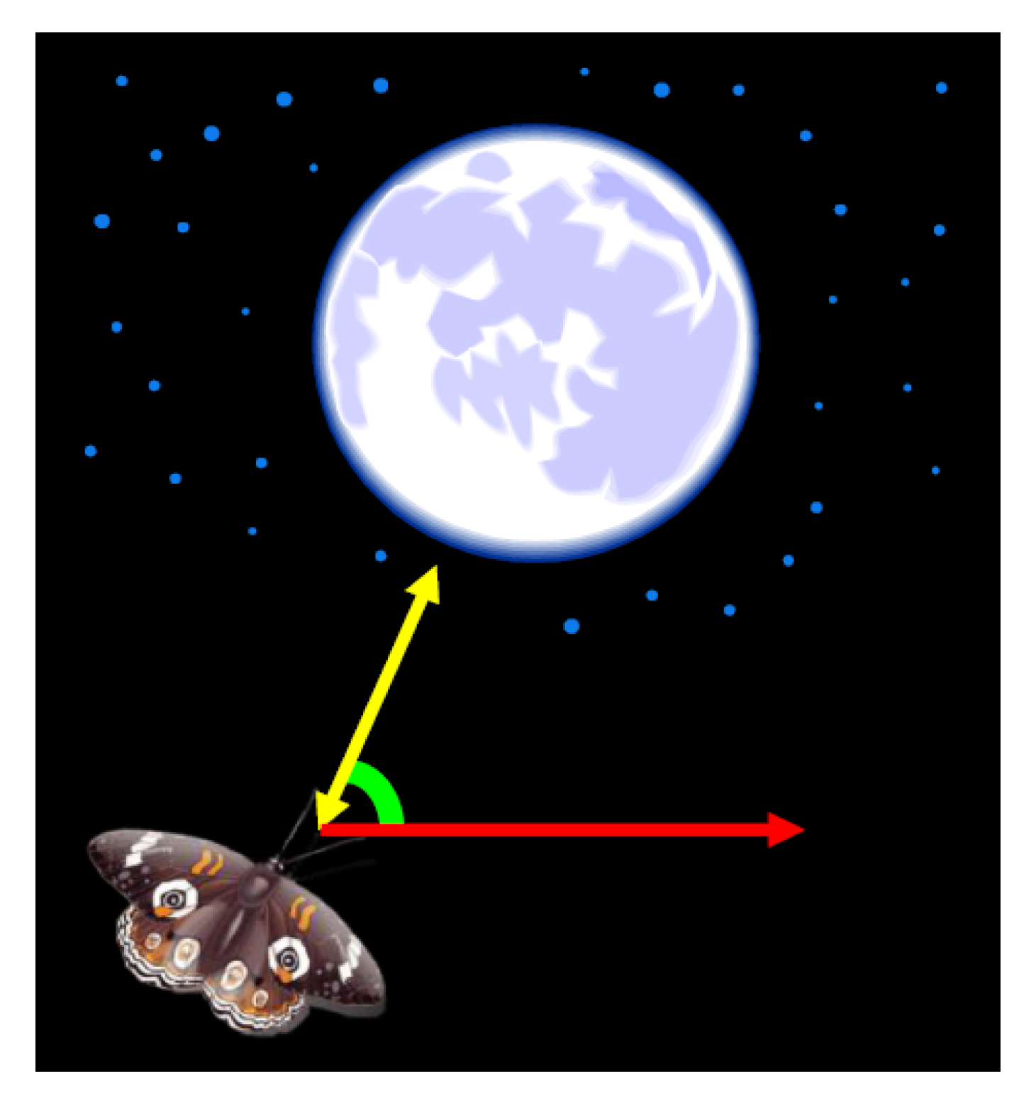
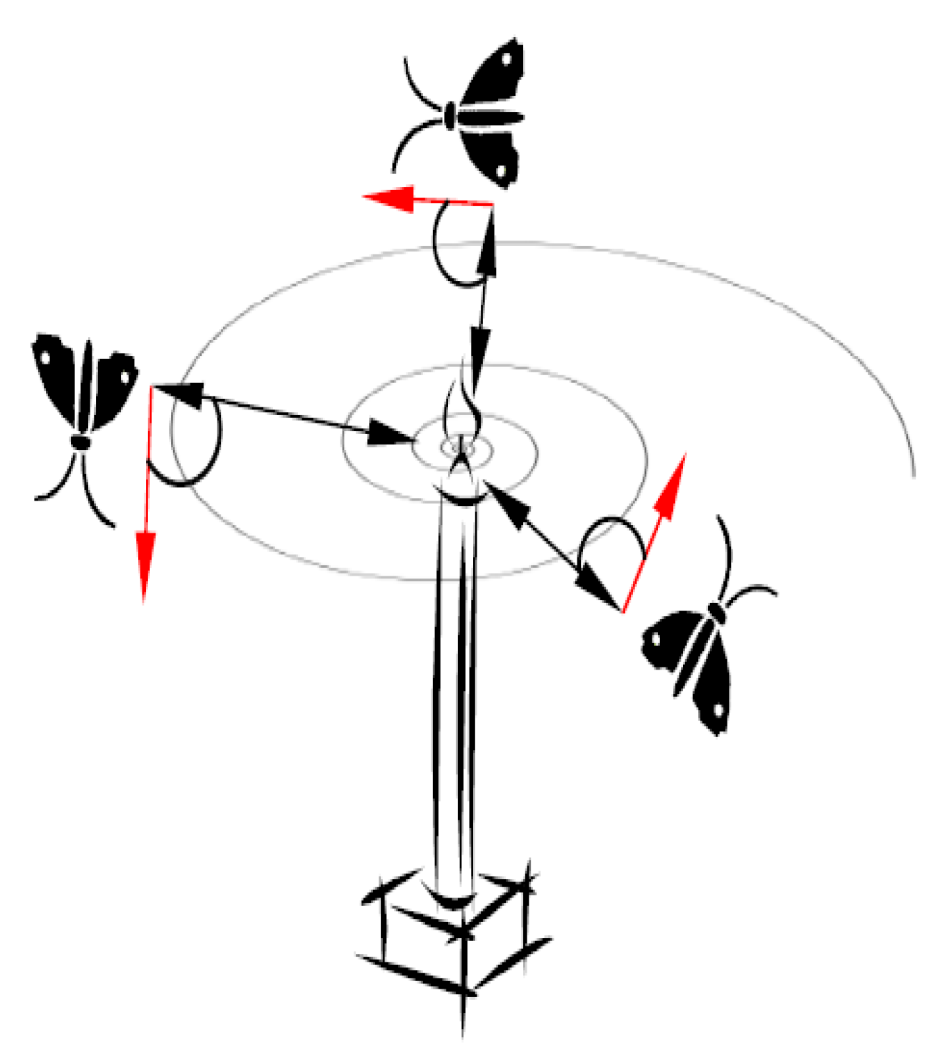
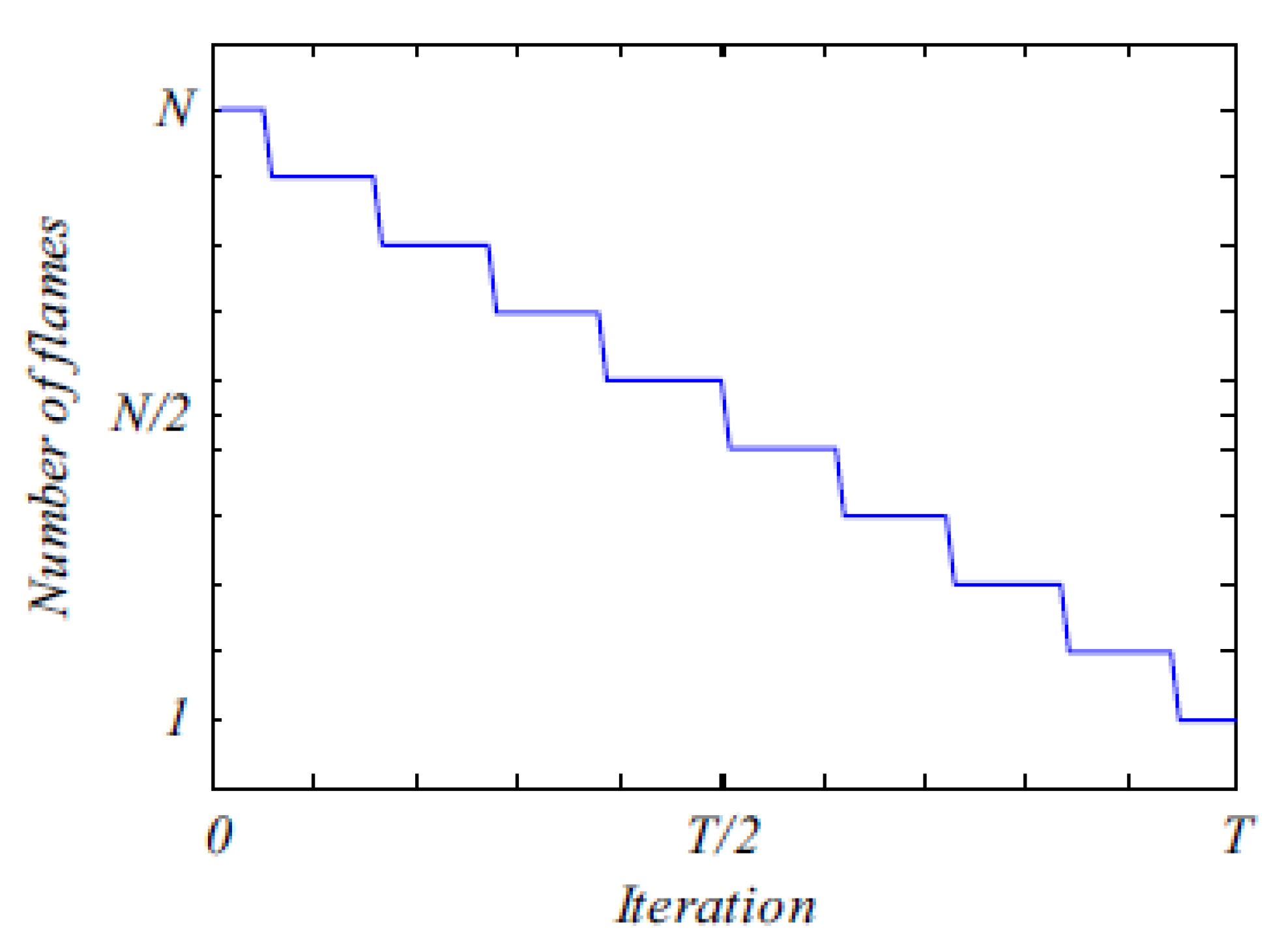
2.2. Moth-Flame Optimization Algorithm (MFO)

Inspired by the navigation method of moths in nature called transverse orientation, Mirjalili proposed a new intelligent optimization method named Moth-flame optimization algorithm (MFO) in 2015. In this method, a moth flies by maintaining a fixed angle with respect to the moon, which is a highly effective mechanism for travelling long distance in a straight path. A conceptual model of transverse orientation is shown in Figure 1. As the moon keeps a long distance from the moth, this mechanism guarantees flying in straight line. Despite the effectiveness of transverse orientation, what we usually observe is that moths fly spirally around artificial lights, which is due to the inefficiency of the transverse orientation, in which it can only help for moving in straight line when the light source is very far. When moths see an artificial light, they also try to keep a similar angle with the light to fly in straight line. Since such a light is extremely close compared to the moon, maintaining a similar angle to the light source will cause the moth to eventually converge towards the light, which can be illustrated in Figure 2 [54].
Figure 1. Transverse orientation.
Applsci 06 00020 g001
Figure 2. Spiral flying path around close light sources.
Applsci 06 00020 g002
According to the behavior of converging towards an artificial light, the steps of the MFO are listed below.
Step 1:
Parameters setting.
The primary parameters of MFO include: the number of moths and flames, Agents_no; the number of variables, dim; the maximum iteration number, Max_iteration; and the lower bound, l b = [ l b 1 , l b 2 , l b 3 , .... , l b n 1 , l b n ] , and upper bound, u b = [ u b 1 , u b 2 , u b 3 , , u b n 1 , u b n ] of variables.
Step 2:
Position initialization.
The position of moths and flames are indicated as Equations (14) and (15), respectively:
M = [ m 1 , 1 m 1 , 2 ... ... m 1 , d m 2 , 1 m 2 , 2 ... ... m 2 , d m n , 1 m n , 2 m n , d ]
F = [ F 1 , 1 F 1 , 2 ... ... F 1 , d F 2 , 1 F 2 , 2 ... ... F 2 , d F n , 1 F n , 2 F n , d ]
where M is the position matrix of moths; F is the position matrix of flames; n is the number of moths; and d is the number of variables (dimensions).
The initialization of M and F can be calculated by
m * , j  or  F * , j = ( u b j l b j ) × r a n d ( ) + l b j
where m * , j and F * , j implies the values of the j-th column of the matrix M and F, respectively; rand is the random number generated with uniform distribution in the interval [0, 1]; and u b j and l b j indicate the upper bound and lower bound of j-th variable, respectively.
Step 3:
Fitness value selection.
To evaluate each flame, a fitness function that can generate fitness values by inputting the position of flames would be given during optimization, and the matrix OF is employed to store the corresponding fitness values of flames.
O F = [ O F 1 O F 2 O F n ]
where OF is the matrix for saving the fitness value of flames, and n indicates the number of moths.
Selecting and saving the fitness value will make a moth never lose the best solutions in each iteration. With the purpose of increasing the probability of finding better solutions, the best solutions obtained so far are considered as the flames. Therefore, the matrix OF always includes n recent best solutions obtained thus far.
Step 4:
Iteration start.
In order to mathematically model the behavior of converging towards the light, a logarithmic spiral is defined for the MFO algorithm to simulate the spiral flying path of moths with respect to a flame:
M i = S ( M i , F j ) = D i e b t cos ( 2 π t ) + F j
D i can be calculated as follows:
D i = | F j M i |
where M i indicates the i-th moth, F j indicates the j-th flame, S is the spiral function, D i indicates the distance of the i-th moth for j-th flame, b is a constant for defining the shape of logarithmic spiral, and t is a random number in [–1, 1].
As the primary component of MFO method, the spiral movement illustrates how the moths update their positions around a flame. The t parameter in the spiral equation implies how much the next position of the moth should be close to the flame (t = −1 shows the closest position to the flame, while t = 1 indicates the farthest).
However, the position updating in Equation (18) only requires the moths to move around a flame, which causes the MFO algorithm to be converged in local optima quickly. To avoid local optimum stagnation, each moth is obliged to update its position according to only one of the flames in Equation (18). In each iteration and after updating the list of flames, the flames are sorted based on their fitness values. Then, the moths update their positions with respect to their corresponding flames.
However, the position updating of moths with respect to n different locations in the search space will possibly degrade the exploitation of best promising solutions. In order to solve this, an adaptive mechanism is carried out for the number of flames. Figure 3 described the way that the number of flames is declined adaptively during the course of iterations. The formula which is employed in this regard is as follows:
f l a m e _ n o = r o u n d ( N l × N 1 T )
where l implies the current number of iteration, N indicates the maximum number of flames, and T is the maximum number of iterations.
Figure 3. Number of flame is declined adaptively during the course of iterations.
Applsci 06 00020 g003
Step 5:
Optimal flames selection.
The position of the flame would be updated if any of the moths becomes fitter than it. According to this rule, the position and the fitness of flames would be updated, and then re-determine the best flame and update its position if any moth becomes fitter than the best flame selected from the previous iteration. When the iteration criterion is met, the best solution would be returned as the best obtained approximation of the optimum.

3. Rolling-MFO-GM (1,1) Model
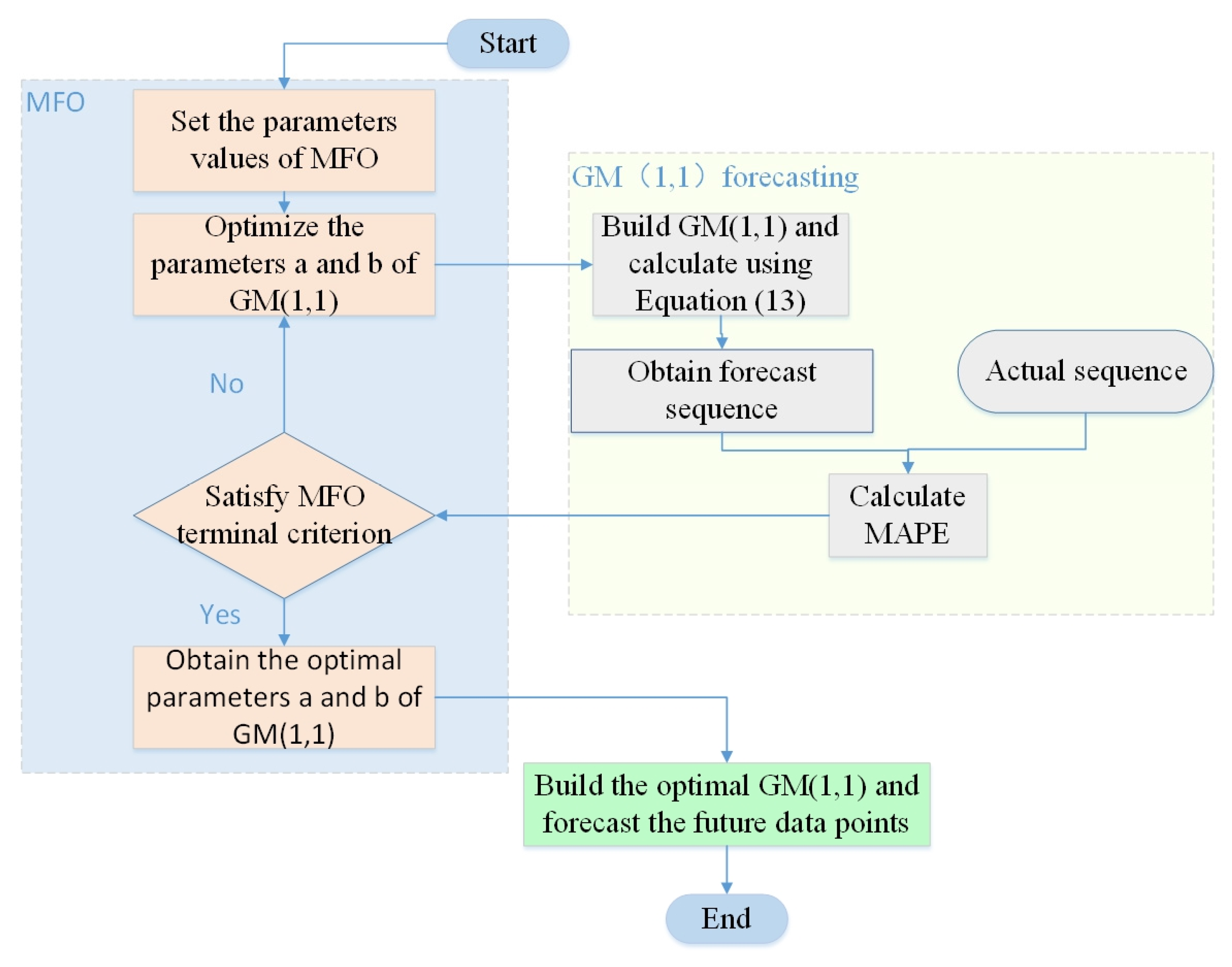
This paper proposed a new optimized grey forecasting model named Rolling-MFO-GM (1,1), which uses MFO to optimize the parameters of GM (1,1), and also employs the rolling mechanism to improve the predicting precision. The principle of Rolling-MFO-GM (1,1) is represented as follows.

3.1. MFO-GM (1,1)

Generally, the parameters a and b of GM (1,1) are usually determined by the least square estimation method [56]. However, as the accuracy of forecasting is required to be enhanced, many scholars have employed various kinds of methods to optimize these two parameters, such as intelligent optimization algorithms, which can improve the forecasting performance of grey model. In this paper, the two parameters of GM (1,1) are optimally determined by MFO on the purpose of improving the accuracy of annual electricity consumption. The procedures of MFO-GM (1,1) are elaborated below.
Step 1:
Parameters initialize.
Five parameters should be set firstly, which are the number of moths and flames, Agents_no; the number of variables, dim; the maximum iteration number, Max_iteration; and the lower bound, l b = [ l b 1 , l b 2 , l b 3 , .... , l b n 1 , l b n ] , and upper bound, u b = [ u b 1 , u b 2 , u b 3 , .... , u b n 1 , u b n ] , variables. In this paper, it is assumed that Agents_no = 100, dim = 2, Max_iteration = 1000, lb = [−10, 10], ub = [0, 10,000].
Step 2:
Optimization starts.
When employing MFO to optimize the parameters of GM (1,1), the fitness function should be determined firstly. This paper uses the Mean Absolute Percentage Error (MAPE, shown as Equation (21)) to build the fitness function.
M A P E = 1 n k = 1 n | x ( k ) x ( k ) x ( k ) | × 100 %
where x ( k ) is the practical value at time k; and x ( k ) is the forecasting value at time k.
In MFO-GM (1,1), the parameters a and b are determined by the position of flames stored in the column vector OF. According to the initialization position generated by Equation (16), GM (1,1) can be built, and Equation (13) can be calculated. The actual data sequence { x ( 0 ) ( 1 ) , x ( 0 ) ( 2 ) , , x ( 0 ) ( p ) } is selected as the input sequence, and then the forecasting sequence { x ( 0 ) ( 1 ) , x ( 0 ) ( 2 ) , , x ( 0 ) ( p ) } can be calculated in accordance with the GM (1,1). Furthermore, the fitness function can be confirmed which minimizes the result of MAPE of forecasting data elements, which is defined as follow:
f = min 1 p k = 1 p | x ( 0 ) ( k ) x ( 0 ) ( k ) x ( 0 ) ( k ) | × 100 %
Up to now, the best solution can be selected at the first iteration. The next 999 iterations (the maximum iterations, 1000, minus the initial iteration, 1) will be carried out on the basis of this optimization mechanism of MFO.
Step 3:
Optimization ends.
In the process of optimization, different MAPEs would be generated due to the different parameters values, and the best MAPE could be found by the end of the optimization. Furthermore, the optimal parameters a and b could be calculated by MFO based on Equation (22). Then, the future data can be forecasted by substituting the optimal parameters a and b into Equation (13).
The process of MFO-GM (1,1) is illustrated in Figure 4.
Figure 4. Flow process diagram of grey model (1,1) optimized by moth-flame optimization algorithm (MFO-GM (1,1)).
Applsci 06 00020 g004

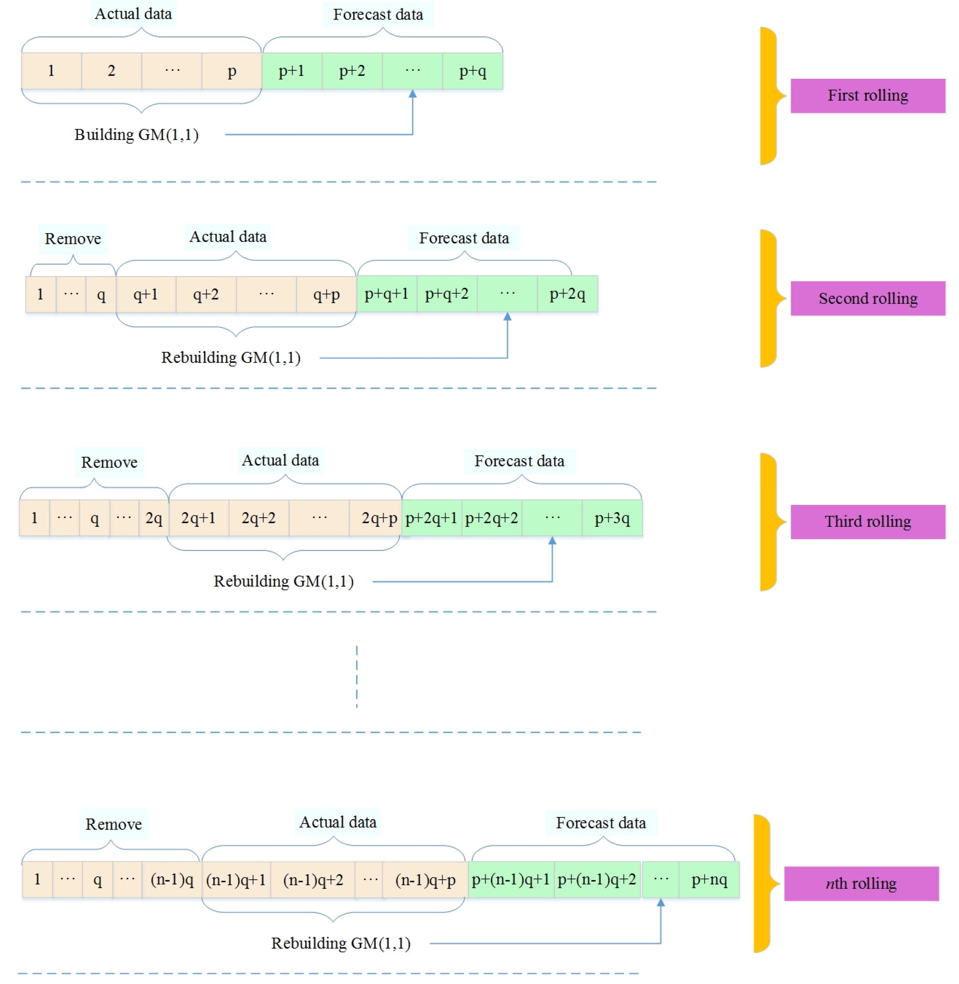
3.2. Rolling-GM (1,1)

The procedures of rolling-GM (1,1) are much more complicated than those of GM (1,1). Since the rolling mechanism focuses on utilizing recent data to predict future electricity demand, which can exhibit the latest development of economic and society, it can enhance the accuracy of forecasting results to a great extent [33,40].
It is assumed that p data elements are used as the input sequence of GM (1,1), and q data elements are to be forecasted by GM (1,1) in each rolling course. The procedures of rolling-GM (1,1) can be summarized below.
Step 1:
sequence { x ( 0 ) ( 1 ) , x ( 0 ) ( 2 ) , , x ( 0 ) ( p ) } is initially utilized as the input sequence of GM (1,1), and then data elements { x ( 0 ) ( p + 1 ) , x ( 0 ) ( p + 2 ) , , x ( 0 ) ( p + q ) } can be predicted.
Step 2:
As the rolling mechanism focused on updating data with the most recent ones, GM (1,1) needs to be rebuilt with p new actual data elements. In order to forecast the data elements { x ( 0 ) ( p + q + 1 ) , x ( 0 ) ( p + q + 2 ) , , x ( 0 ) ( p + 2 q ) } , the sequence { x ( 0 ) ( 1 ) , x ( 0 ) ( 2 ) , , x ( 0 ) ( p ) } need to be replaced by the latest p data elements { x ( 0 ) ( q + 1 ) , x ( 0 ) ( q + 2 ) , , x ( 0 ) ( q + p ) } , which would be employed to rebuild GM (1,1).
Step 3:
Repeat Step 2 until all the data elements that need to be forecasted are obtained.
The forecasting procedure of rolling-GM (1,1) is illustrated in Figure 5.
Figure 5. Forecasting procedure of rolling-GM (1,1).
Applsci 06 00020 g005

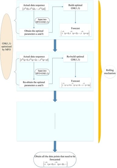
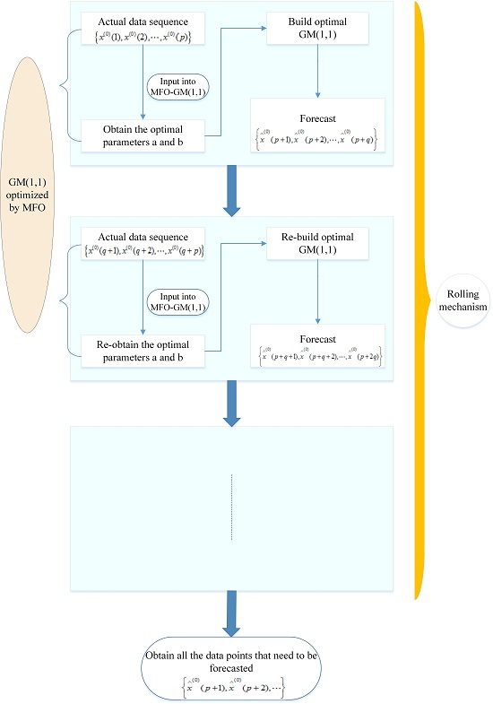
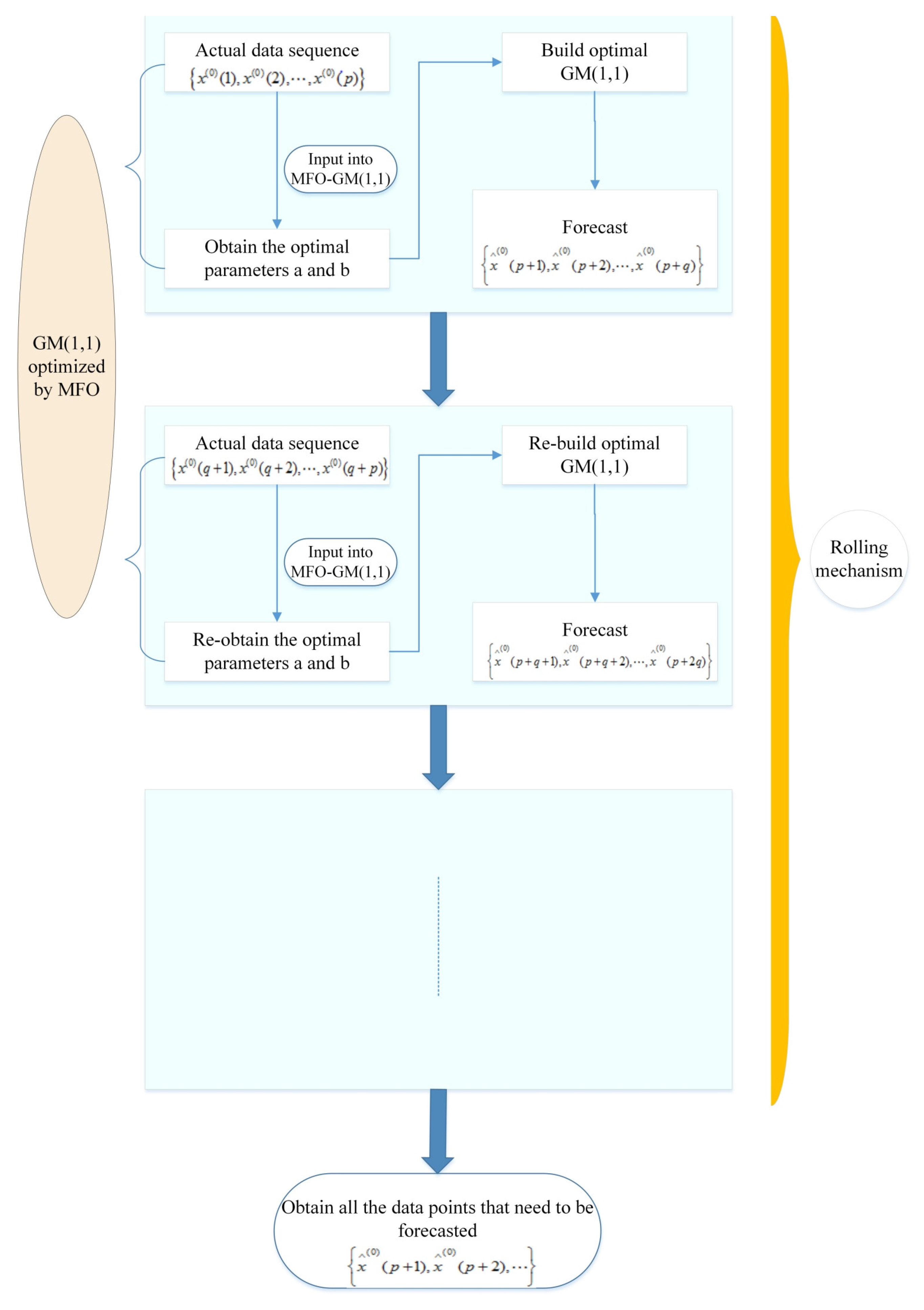
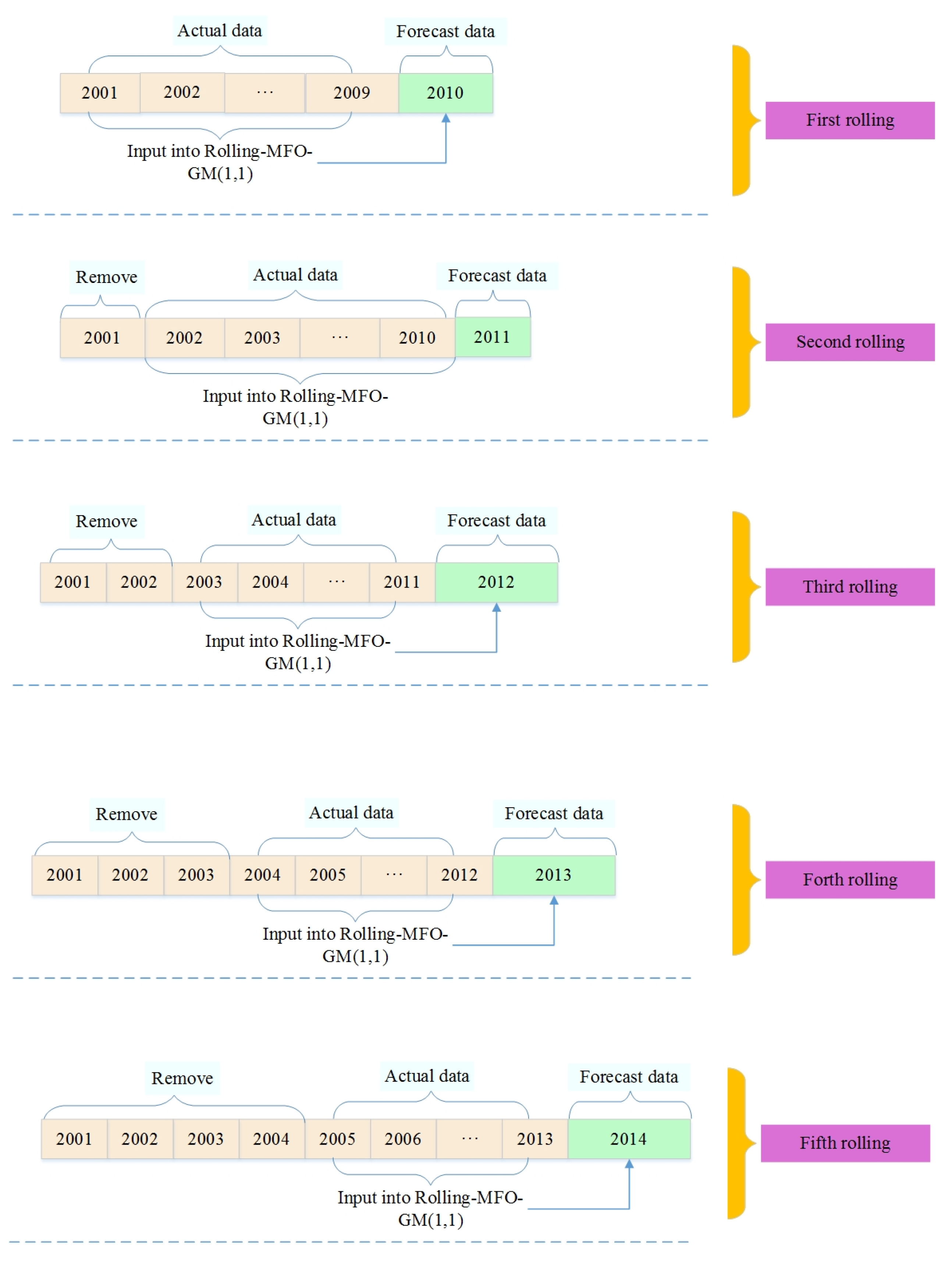
3.3 Rolling-MFO-GM (1,1)

Rolling-MFO-GM (1,1) is much more complex than GM (1,1) and MFO-GM (1,1), in which the parameters of GM (1,1) are optimized by MFO and the rolling mechanism is also introduced to enhance the precision of forecasting results. The steps of Rolling-MFO-GM (1,1) are listed as follows.
Step 1:
The actual data sequence { x ( 0 ) ( 1 ) , x ( 0 ) ( 2 ) , , x ( 0 ) ( p ) } is utilized to build MFO-GM (1,1), and then the optimal parameters a and b could be calculated by MFO using Equation (22). Then the forecasting sequence { x ( 0 ) ( p + 1 ) , x ( 0 ) ( p + 2 ) , , x ( 0 ) ( p + q ) } can be calculated using Equation (13).
Step 2:
As the rolling mechanism aims at employing the latest data for forecasting; in this step, MFO-GM (1,1) should be rebuilt using the new practical data sequence { x ( 0 ) ( q + 1 ) , x ( 0 ) ( q + 2 ) , , x ( 0 ) ( q + p ) } . Then, the parameters a and b would be re-optimized by MFO using Equation (23) and the forecasting sequence { x ^ ( 0 ) ( p + q + 1 ) , x ^ ( 0 ) ( p + q + 2 ) , , x ^ ( 0 ) ( p + 2 q ) } can be calculated using Equation (13).
f = min 1 p k = 1 p | x ( 0 ) ( q + k ) x ( 0 ) ( q + k ) x ( 0 ) ( q + k ) | × 100 %
Step 3:
Repeat Step 2 until all the forecasting data points are obtained.
The procedure of Rolling-MFO-GM (1,1) is illustrated in Figure 6.
Figure 6. The flow process diagram of Rolling-MFO-GM (1,1).
Applsci 06 00020 g006

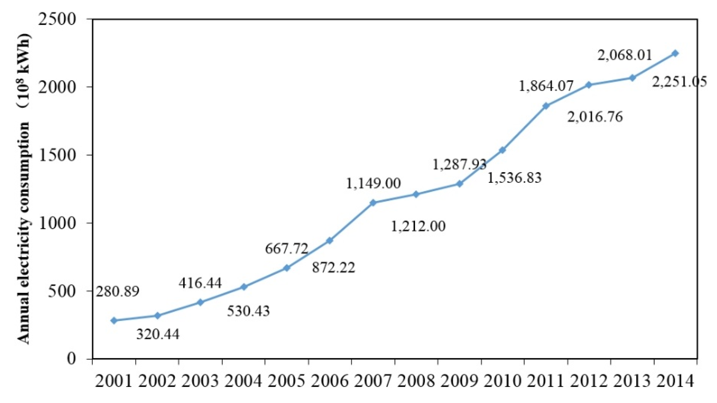
4. Forecasting Annual Electricity Consumption by Employing Rolling-MFO-GM (1,1) Model

In this paper, Rolling-MFO-GM (1,1) is applied to forecast the electricity consumption of Inner Mongolia, China. The electricity consumption of energy-intensive industries accounts for a significant share of total electricity demand of Inner Mongolia, so accurately forecasting electricity consumption will contribute to the sustainable development of regional industry and electric power grid. The sample data, the annual electricity consumption of Inner Mongolia between 2001 and 2014, are collected from North China Electric Power Statistical Yearbook. The changing trend of these 14 data is shown in Figure 7. This paper set p = 9 and q = 1 , which implies nine data points are used as the input sequence feeding into Rolling-MFO-GM (1,1), and one data point needs to be forecasted. The primary reason for using nine data points is that its forecasting result performs better than using other data sequences, such as five data points, six data points or eight data points, namely the forecasting result of using nine data points is much closer to the actual value. The detailed procedures of predicting electricity consumption of Inner Mongolia is displayed in Figure 8. It can be drawn that the parameters of a and b can be optimized after five times rolling. Therefore, five groups of parameters a and b can be obtained.
Figure 7. Annual electricity consumption of Inner Mongolia between 2001 and 2014.
Applsci 06 00020 g007
Figure 8. Forecasting procedure of Inner Mongolia’s electricity consumption employing Rolling-MFO-GM (1,1) model.
Applsci 06 00020 g008
Five sets of optimal parameters a and b for electricity consumption forecasting of Inner Mongolia from 2010 to 2014 are shown in Table 1. Then, the electricity consumption between 2010 and 2014 can be forecasted using Equation (13), which is also shown in Table 1.
Table 1. Optimal parameters’ values and forecasting results by using rolling-MFO-GM (1,1).
YearParametersForecasting ValueActual ValueThe Gap
ab
2010−0.2137241.66291546.381536.83−9.55
2011−0.1774349.10431881.121864.07−17.05
2012−0.1711444.68202189.212016.76−172.45
2013−0.1416629.60032315.542068.01−247.53
2014−0.1341750.48582462.042251.05−210.99
The gap means the different between the forecasting value and actual value. Of which, the negative value indicates the forecasting value is larger than the actual value.

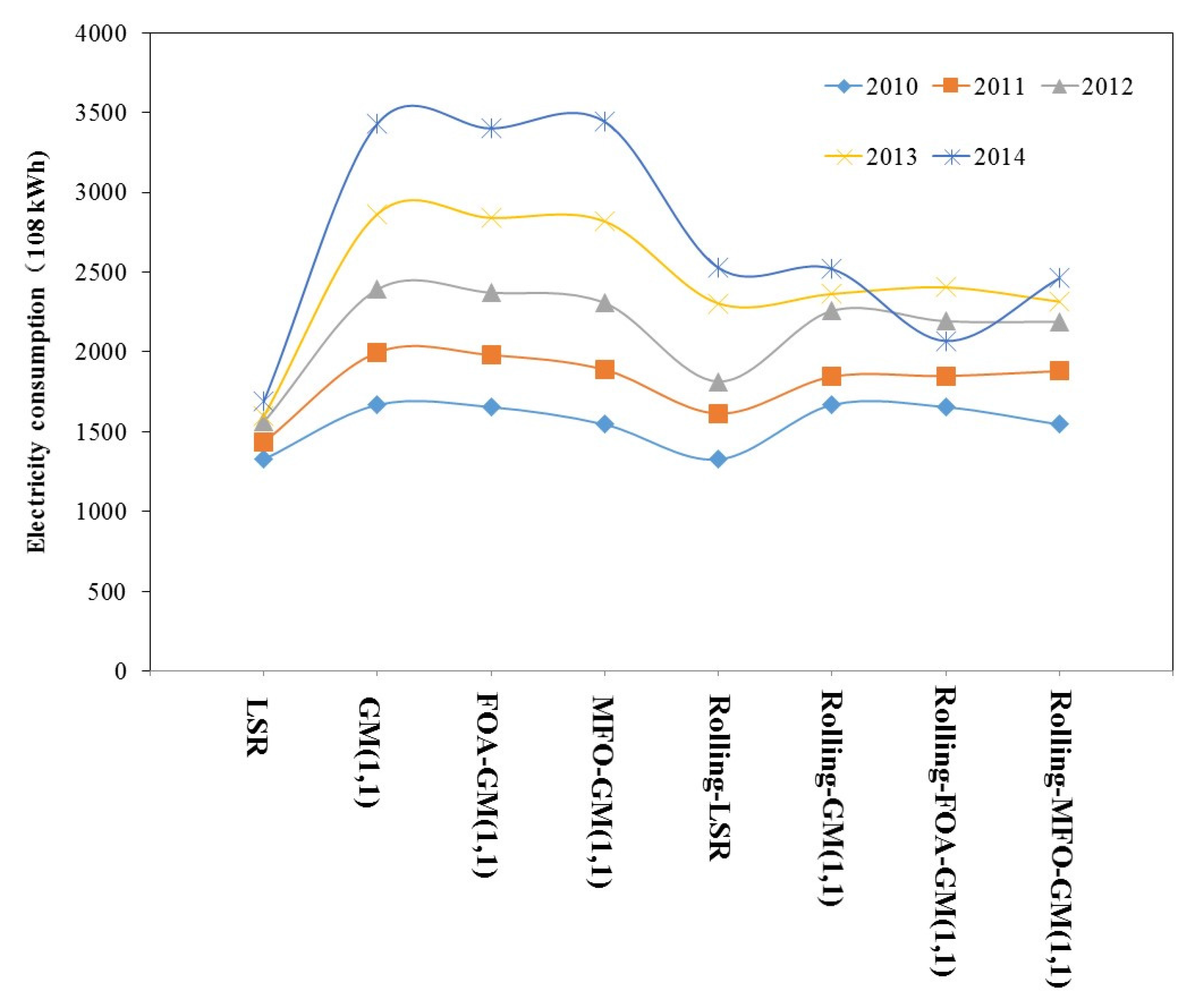
5. Comparison of Forecasting Results by Different Forecasting Models

With the aim of evaluating the precision of Rolling-MFO-GM (1,1) model for annual electricity consumption forecasting, the LSR (least square regression) method, GM (1,1), FOA (fruit fly optimization)-GM (1,1), MFO-GM (1,1), Rolling-LSR, Rolling-GM (1,1) and Rolling-FOA-GM (1,1) are selected as the compared models. Among these models, LSR method, GM (1,1), FOA-GM (1,1) and MFO-GM (1,1) are a class of forecasting models without rolling mechanism, while Rolling-LSR, Rolling-GM (1,1), Rolling-FOA-GM (1,1) and Rolling-MFO-GM (1,1) are another class of forecasting models with rolling mechanism. Specifically, LSR method, which is not a grey-based forecasting technique, is selected to validate the effectiveness of the proposed approach.
As the most well-known linear model in statistics and mathematics, LSR method is an effective technique to realize correlation analysis between variables. Given a set of training samples, LSR can find the coefficients of a linear model by minimizing the residual sum of squares [57]. For LSR method, the electricity consumption data points from 2001 to 2009 of Inner Mongolia will be treated as the training samples. The regression coefficient a and constant term b are shown in Table 2. According to the regression model, the forecasting values can be obtained (see Table 3).
For GM (1,1), the input data sequence is the electricity consumption data from 2001 to 2009 of Inner Mongolia, and then the parameters a and b can be determined (see Table 2). On the basis of this, the forecasting results of 2010–2014 can be calculated using Equation (13) (see Table 3).
For FOA-GM (1,1), the optimization algorithm FOA is applied to iteratively select the optimal value of parameters a and b of GM (1,1). Before iteration, the original parameters of FOA are set as follows: maxgen = 100, sizepop = 20, ( X _ axis ,   Y _ axis ) [- 50 , 50 ] , FR [- 10 , 10 ] , X _ axis = rands ( 1 , 2 ) , Y _ axis = rands ( 1 , 2 ) . The values of parameters a and b optimized by FOA are listed in Table 2, and the prediction results are shown in Table 3.
For MFO-GM (1,1), the forecasting procedure is shown as Figure 4. Applying the electricity consumption from 2001 to 2009 as input sequence, the parameters a and b can be optimized by MFO. Before iteration, the initial parameters setting are same as that in Section 3.2. Then, we can use the optimal values of a and b which are itemized in Table 2 to calculate the electricity consumption of 2010–2014, and the results are shown in Table 3.
For Rolling-LSR, we can obtain five regression models using five groups of data sequence. The electricity consumption from 2001 to 2009 are treated as the input sequence of LSR, so the electricity consumption of 2010 can be calculated based on the first regression model. Then, the data from 2002 to 2010 are employed as input sequence, so the electricity consumption of 2011 can be forecasted on the basis of the second regression model, and so on. Finally, five regression models can be obtained, and the electricity consumption from 2010 to 2014 can be forecasted, which are shown in Table 3.
Table 2. The parameters’ values determined by different compared forecasting models.
YearLSRGM (1,1)FOA-GM (1,1)MFO-GM (1,1)Rolling-LSRRolling-GM (1,1)Rolling-FOA-GM (1,1)
ababababababab
2010128.829239.4175−0.1821313.86480.1808307.2826−0.2137241.6629128.829239.4175−0.1821313.8648−0.1808307.2826
2011150.4075111.0747−0.1622422.0084−0.1730381.0492
2012162.1653193.8000−0.1554512.346−0.2041316.606
2013198.3753350.5633−0.1404644.246−0.2152310.4759
2014199.8292529.1364−0.1172828.0705−0.06531094.4900
Table 3. The forecasting results of different compared models.
YearActual ValueLSRGM (1,1)FOA-GM (1,1)MFO-GM (1,1)Rolling-LSRRolling-GM (1,1)Rolling-FOA-GM (1,1)
Forecasting ValueThe GapForecasting ValueThe GapForecasting ValueThe GapForecasting ValueThe GapForecasting ValueThe GapForecasting ValueThe GapForecasting ValueThe Gap
20101536.831327.72209.111668.59−131.761654.8−117.971546.38−9.551327.72209.111668.59−131.761654.8−117.97
20111864.071434.55429.521997.67−133.61981.16−117.091888.76−24.691615.17248.901845.9618.111849.6614.41
20122016.761561.38455.382391.64−374.882371.88−355.122306.93−290.171815.5201.262258.21−241.452192.67−175.91
20132068.011597.21470.802863.32−795.312839.65−771.642817.69−749.682334.36−266.352363.73−295.722404.58−336.57
20142251.051689.04562.013428.01−1176.963399.68−1148.633441.54−1190.492527.44−276.392520.12−269.072069.51181.54
The gap means the different between the forecasting value and actual value. Of which, the positive value of the gap indicates the actual value is larger than the forecasting value, while the negative value indicates the forecasting value is larger than the actual value.
For Rolling-GM (1,1), the forecasting procedure is illustrated in Figure 5. We use the electricity consumption from 2001 to 2009 as the input sequence of GM (1,1), and the first group of parameters a and b can be obtained, then the electricity consumption of 2010 can be calculated. After that, the data of 2002–2010 are utilized as input sequence, and the second group of parameters a and b can be obtained, then the electricity consumption of 2011 can be forecasted. The rest can be done in the same manner. Finally, five groups of parameters a and b and the forecasted electricity consumption of 2010–2014 can be obtained (see Table 3).
For Rolling-FOA-GM (1,1), the procedure of prediction is the same as Rolling-MFO-GM (1,1). The only difference between these two models is the meta-heuristic algorithm employed to optimize the parameters a and b of GM (1,1). The five groups of optimized values of parameters a and b obtained by FOA in each iteration are listed in Table 2. The forecasting results are listed in Table 3.
The forecasting results of electricity consumption of Inner Mongolia from 2010 to 2014, utilizing the different models above, are illustrated in Figure 9.
Figure 9. Forecasting results of Inner Mongolia’s electricity consumption from 2010 to 2014 by different models.
Applsci 06 00020 g009
As can be seen in Figure 9, the models with rolling mechanism show a better forecasting performance than the models without rolling mechanism. Specially, the forecasted annual electricity consumption using GM (1,1), FOA-GM (1,1) and MFO-GM (1,1) are much higher than actual electricity consumption, while the forecasting results of Rolling-LSR, Rolling-GM (1,1), Rolling-FOA-GM (1,1), and Rolling-MFO-GM (1,1) are much closer to actual values. Without rolling mechanism, the further into the future, the more the forecasted annual electricity consumption deviates from the actual annual electricity consumption. However, a forecast with rolling mechanism can pull it back at each “roll”. The primary reason is that a rolling forecast can use more up-to-date information, which takes not only the latest development of policy, the economy and society into account but also the features of forecasting objective into consideration. Therefore, the accuracy of forecasting results with rolling mechanism can be remarkably improved. This finding has also been verified in other practical issues, such as the prediction of GDP, interest rate, and energy consumption [42,58]. Additionally, the forecasting performance of MFO-GM (1,1) is much better to that of LSR, GM (1,1) and FOA-GM (1,1), which implies using MFO to optimize the parameters of GM (1,1) is effective and promising.
To further evaluate the accuracy of each forecasting model, several evaluation indicators are selected to analyze the accuracy of forecasting results, namely Percentage Error (PE), Mean Absolute Percentage Error (MAPE), and Root Mean Square Error (RMSE), which can be calculated as Equations (24)–(26), respectively.
P E = x ( k ) x ( k ) x ( k ) × 100 %
M A P E = 1 n k = 1 n | x ( k ) x ( k ) x ( k ) | × 100 %
R M S E = 1 n k = 1 n ( x ( k ) x ( k ) ) 2
where x ( k ) is the actual value at time k, and x ( k ) is the forecasting value at time k.
The PE results of different forecasting models show the superior performance of Rolling-MFO-GM (1,1) when compared with that of other seven models, as shown in Table 4.
Table 4. Percentage Error (PE) comparison of eight forecasting models.
YearLSRGM (1,1)FOA-GM (1,1)MFO-GM (1,1)Rolling-LSRRolling-GM
(1,1)
Rolling-FOA-GM (1,1)Rolling-MFO-GM (1,1)
201013.61%−8.57%−7.68%−0.62%13.61%−8.57%−7.68%−0.62%
201123.04%−7.17%−6.28%−1.32%13.35%0.97%0.77%−0.91%
201222.58%−18.59%−17.61%−14.39%9.98%−11.97%−8.72%−8.55%
201322.77%−38.46%−37.31%−36.25%−12.88%−14.30%−16.27%−11.97%
201424.97%−52.28%−51.03%−52.89%−12.28%−11.95%8.06%−9.37%
The results of MAPE and RMSE shown in Table 5 verify again that the forecasting models with rolling mechanism perform better than that without rolling mechanism. Furthermore, as can be seen in Table 5, the MAPE value of LSR is smaller than GM (1,1) but much larger than MFO-GM (1,1), which indicates that the MFO algorithm is effective. Meanwhile, according to the evaluating criterion of MAPE listed in Table 6 [33], as the MAPE results of the forecasting models with rolling mechanism are smaller than 10%, the forecasting power of these models is excellent, while the MAPE results of the models without rolling mechanism are a little more than 20%, which indicate the forecasting power of these models is reasonable. What is more, the Rolling-MFO-GM (1,1) is the best forecasting model for annual electricity consumption due to its obtained smallest MAPE (6.29%). We can draw the same conclusions from the results of RMSE as that of MAPE.
Table 5. Results of Mean Absolute Percentage Error (MAPE) and Root Mean Square Error (RMSE) for different forecasting models.
ModelLSRGM (1,1)FOA-GM (1,1)MFO-GM (1,1)Rolling-LSRRolling-GM (1,1)Rolling-FOA-GM (1,1)Rolling-MFO-GM (1,1)
MAPE21.39%25.01%23.98%21.09%12.42%9.55%8.30%6.29%
RMSE441.16662.34643.2642.52235.98 217.18195.6164.87
Table 6. Criterion of MAPE [33].
MAPE (%)Forecasting Power
<10Excellent
10–20Good
20–50Reasonable
>50Incorrect
Above all, the superiority of Rolling-MFO-GM (1,1) can be safely concluded. The proposed Rolling-MFO-GM (1,1), in which the parameters of GM (1,1) are optimized by employing the new intelligent optimization algorithm MFO and the introduction of rolling mechanism, is of great practical significance. Meanwhile, it can also be seen that MFO-GM (1,1) performs better than LSR, GM (1,1) and FOA-GM (1,1), and Rolling-MFO-GM (1,1) is better than Rolling-LSR, Rolling-GM (1,1) and Rolling-FOA-GM (1,1) in terms of annual electricity consumption forecasting. These findings indicate that the utilization of MFO to optimize the parameters of GM (1,1) can greatly enhance the precision of annual electricity consumption forecasting. Additionally, as the rolling mechanism uses recent data as input sequence of forecasting model, which can consider the latest change trends of policy, economy and society as well as the characteristics of forecasting subject, the models with rolling mechanism can perform better than those without rolling mechanism in terms of annual electricity consumption forecasting.

6. Conclusions

Accurate and reliable forecasting on annual electricity consumption will be valuable for social projectors and power network operators. For the purpose of enhancing the accuracy of electricity consumption prediction, this paper proposed a new hybrid optimized grey model named Rolling-MFO-GM (1,1), which combines rolling mechanism, the latest intelligent optimization algorithm MFO and grey forecasting model GM (1,1). What we can conclude from the empirical analysis are as follows:
(1)
Employing MFO to optimize the parameters of GM (1,1) can enhance the accuracy of annual electricity consumption prediction significantly.
(2)
The introduction of rolling mechanism can also make the forecasting results much closer to the actual data.
Currently, many scholars focus on the combination of GM (1,1) with various kinds of intelligent optimization algorithms or with rolling mechanism. Therefore, this paper combines GM (1,1), intelligent optimization algorithm MFO, and rolling mechanism together, attempting to improve the forecasting accuracy of annual electricity consumption. In future research, MFO can be employed to optimize support vector machines, the weight coefficients of combination forecasting models, and neural network for other forecasting issues, such as short-term electric power load forecasting, wind speed forecasting, and so on.

Acknowledgments

This study is supported by the National Natural Science Foundation of China under Grant No. 71373076, and the Fundamental Research Funds for the Central Universities under Grant No. 2015 XS28.

Author Contributions

Huiru Zhao and Sen Guo designed and proposed the concept of this research. Haoran Zhao completed the paper. Sen Guo also refined the manuscript and revised the final draft of the manuscript.

Conflicts of Interest

The authors declare no conflict of interest.

References

  1. Hamzacebi, C.; Es, H.A. Forecasting the annual electricity consumption of Turkey using an optimized grey model. Energy 2014, 70, 165–171. [Google Scholar] [CrossRef]
  2. Swan, L.G.; Ugursal, V.I. Modeling of end-use energy consumption in the residential sector: A review of modeling techniques. Renew. Sustain. Energy Rev. 2009, 13, 1819–1835. [Google Scholar] [CrossRef]
  3. Qin, H.-T.; Liu, Y.; Xiao, H.; Dang, Z.; Yang, S.; Wang, H. Forecast of medium and long-term power demand and distribution in Chongqing. Electr. Power Constr. 2015, 4, 115–122. [Google Scholar]
  4. Ning, B.; Kang, C.; Xia, Q. The expansion strategy for medium and long term load forecasting model. China Power 2000, 10, 38–40. [Google Scholar]
  5. Bianco, V.; Manca, O.; Nardini, S. Electricity consumption forecasting in Italy using linear regression models. Energy 2009, 34, 1413–1421. [Google Scholar] [CrossRef]
  6. Bianco, V.; Manca, O.; Nardini, S. Linear regression models to forecast electricity consumption in Italy. Energy Sources B Econ. Plan. Policy 2013, 8, 86–93. [Google Scholar] [CrossRef]
  7. Farzana, S.; Liu, M.; Baldwin, A.; Hossain, M.U. Multi-model prediction and simulation of residential building energy in urban areas of Chongqing, South West China. Energy Build. 2014, 81, 161–169. [Google Scholar] [CrossRef]
  8. Dilaver, Z.; Hunt, L.C. Industrial electricity demand for Turkey: A structural time series analysis. Energy Econ. 2011, 33, 426–436. [Google Scholar] [CrossRef] [Green Version]
  9. Hu, L. Study on Short Term Electric Load Forecasting Based on Fuzzy Neural Network; Nan Hua University: China, 2011. [Google Scholar]
  10. Metaxiotis, K.; Kagiannas, A.; Askounis, D.; Psarras, J. Artificial intelligence in short term electric load forecasting: A state-of-the-art survey for the researcher. Energy Convers. Manag. 2003, 44, 1525–1534. [Google Scholar] [CrossRef]
  11. Wang, K.-L.; Yang, L. Study on power demand forecasting based on non-linear regression combined neural network. Comput. Eng. Appl. 2010, 28, 225–227. [Google Scholar]
  12. Azadeh, A.; Ghaderi, S.F.; Sheikhalishahi, M.; Nokhandan, B.P. Optimization of short load forecasting in electricity market of Iran using artificial neural networks. Optim. Eng. 2014, 15, 485–508. [Google Scholar] [CrossRef]
  13. Ma, W.-X.; Bai, X.-M.; Mu, L.-S. Short term load forecasting using artificial neuron network and fuzzy inference. Grid Technol. 2003, 5, 29–32. [Google Scholar]
  14. Chen, T. A collaborative fuzzy-neural approach for long-term load forecasting in Taiwan. Comput. Ind. Eng. 2012, 63, 663–670. [Google Scholar] [CrossRef]
  15. Chen, T.; Wang, Y.-C. Long-term load forecasting by a collaborative fuzzy-neural approach. Int. J. Electr. Power Energy Syst. 2012, 43, 454–464. [Google Scholar] [CrossRef]
  16. AlRashidi, M.R.; El-Naggar, K.M. Long term electric load forecasting based on particle swarm optimization. Appl. Energy 2010, 87, 320–326. [Google Scholar] [CrossRef]
  17. Cong, R.; Zhang, Y.; Zhao, Y. Prediction of Shandong power demands based on the SVM model. Energy Technol. Econ. 2011, 3, 40–45. [Google Scholar]
  18. Cheng, Z.; Chen, X. Adaptive combination forecasting model based on area correlation degree with application to China’s energy consumption. J. Appl. Math. 2014, 2014, 1–13. [Google Scholar] [CrossRef]
  19. Xue, Y.; Cao, Z.; Xu, L. The application of combination forecasting model in energy consumption system. Energy Proc. 2011, 5, 2599–2603. [Google Scholar] [CrossRef]
  20. Liang, N. Short-Term Load Forecasting Based on Modified Fruit Fly Algorithm and Support Vector Machine; Guangxi University: Nanning, China, 2014. [Google Scholar]
  21. Li, X.; Yang, C.; Qi, J. A new support vector machine optimized by improved particle swarm optimization and its application. J. Cent. South Univ. Technol. 2006, 13, 568–572. [Google Scholar] [CrossRef]
  22. Wu, J.; Yang, S.; Liu, C. Parameter selection for support vector machines based on genetic algorithm to short-term power load forecasting. J. Cent. South Univ. 2009, 1, 180–184. [Google Scholar]
  23. Wang, J.; Li, L.; Niu, D.; Tan, Z. An annual load forecasting model based on support vector regression with differential evolution algorithm. Appl. Energy 2012, 94, 65–70. [Google Scholar] [CrossRef]
  24. Zhao, H.; Guo, S.; Xue, W. Urban saturated power load analysis based on a novel combined forecasting model. Information 2015, 6, 69–88. [Google Scholar] [CrossRef]
  25. Deng, J.-L. Introduction to grey system theory. J. Grey Syst. 1989, 1, 1–24. [Google Scholar]
  26. Bahrami, S.; Hooshmand, R.A.; Parastegari, M. Short term electric load forecasting by wavelet transform and grey model improved by PSO (particle swarm optimization) algorithm. Energy 2014, 72, 434–442. [Google Scholar] [CrossRef]
  27. Kang, J.; Zhao, H. Application of improved grey model in long-term load forecasting of power engineering. Syst. Eng. Proc. 2012, 3, 85–91. [Google Scholar] [CrossRef]
  28. Liu, X.; Peng, H.; Bai, Y.; Zhu, Y.; Liao, L. Tourism flows prediction based on an improved grey GM (1,1) model. Proc. Soc. Behav. Sci. 2014, 138, 767–775. [Google Scholar] [CrossRef]
  29. Benítez, R.B.C.; Paredes, R.B.C.; Lodewijks, G.; Nabais, J.L. Damp trend Grey Model forecasting method for airline industry. Expert Syst. Appl. 2013, 40, 4915–4921. [Google Scholar] [CrossRef]
  30. Li, G.D.; Masuda, S.; Nagai, M. The prediction for Japan’s domestic and overseas automobile production. Technol. Forecast. Soc. Chang. 2014, 87, 224–231. [Google Scholar] [CrossRef]
  31. Truong, D.Q.; Ahn, K.K. Wave prediction based on a modified grey model MGM (1,1) for real-time control of wave energy converters in irregular waves. Renew. Energy 2012, 43, 242–255. [Google Scholar] [CrossRef]
  32. El-Fouly, T.H.M.; El-Saadany, E.F.; Salama, M.M.A. Grey predictor for wind energy conversion systems output power prediction. IEEE Trans. Power Syst. 2006, 3, 1450–1452. [Google Scholar] [CrossRef]
  33. Zhao, Z.; Wang, J.; Zhao, J.; Su, Z. Using a grey model optimized by differential evolution algorithm to forecast the per capita annual net income of rural households in China. Omega 2012, 40, 525–532. [Google Scholar] [CrossRef]
  34. Zhou, W.; He, J.M. Generalized GM (1,1) model and its application in forecasting of fuel production. Appl. Math. Model. 2013, 37, 6234–6243. [Google Scholar] [CrossRef]
  35. Pao, H.T.; Fu, H.C.; Tseng, C.L. Forecasting of CO2 emissions, energy consumption and economic growth in China using an improved grey model. Energy 2012, 40, 400–409. [Google Scholar] [CrossRef]
  36. Xu, R.-F.; Liu, Y. Electric Power demand forecasting based on GM (1,1) model in Shanxi province. Mod. Commer. Ind. 2007, 12, 58–59. [Google Scholar]
  37. Zhang, H.-L.; Chen, Y.; Lu, Z.-N. Short-term prediction of electricity demand of Jiangsu province. Sci. Technol. Manag. 2011, 2, 9–11. [Google Scholar]
  38. Zhou, P.; Ang, B.W.; Poh, K.L. A trigonometric grey prediction approach to forecasting electricity demand. Energy 2006, 31, 2839–2847. [Google Scholar] [CrossRef]
  39. Shen, X.; Lu, Z. The application of Grey theory model in the predication of Jiangsu province’s electric power demand. AASRI Proc. 2014, 7, 81–87. [Google Scholar] [CrossRef]
  40. Akay, D.; Atak, M. Grey prediction with rolling mechanism for electricity demand forecasting of Turkey. Energy 2007, 32, 1670–1675. [Google Scholar] [CrossRef]
  41. Tan, L.-Z.; Ouyang, A.; Peng, X.-Y.; Li, E.-X.; Truong, T.K.; Hao, L. A fast and stable forecasting model to forecast power load. Int. J. Pattern Recognit. Artif. Intell. 2015. [Google Scholar] [CrossRef]
  42. Kumar, U.; Jain, V. Time series models (Grey-Markov, Grey Model with rolling mechanism and singular spectrum analysis) to forecast energy consumption in India. Energy 2010, 35, 1709–1716. [Google Scholar] [CrossRef]
  43. Jiang, Y.-C.; Qian, J. Power load forecasting model based on improved GM (1,1) Euler method. J. Kunming Univ. Sci. Technol. (Nat. Sci. Ed.) 2015, 4, 117–122. [Google Scholar]
  44. Eberhart, R.C.; Kennedy, J. A new optimizer using particle swarm theory. In Proceedings of the Sixth International Symposium on Micro Machine and Human Science, Nagoya, Japan, 4–6 October 1995; Volume 1, pp. 39–43.
  45. Clarke, J.; McLay, L.; McLeskey, J.T. Comparison of genetic algorithm to particle swarm for constrained simulation-based optimization of a geothermal power plant. Adv. Eng. Inform. 2014, 28, 81–90. [Google Scholar] [CrossRef]
  46. Dorigo, M.; Birattari, M.; Stützle, T. Ant colony optimization. Comput. Intell. Mag. IEEE 2006, 1, 28–39. [Google Scholar] [CrossRef]
  47. Storn, R.; Price, K. Differential evolution—A simple and efficient heuristic for global optimization over continuous spaces. J. Glob. Optim. 1997, 11, 341–359. [Google Scholar] [CrossRef]
  48. Papadrakakis, M.; Lagaros, N.D.; Tsompanakis, Y. Structural optimization using evolution strategies and neural networks. Comput. Methods Appl. Mech. Eng. 1998, 156, 309–333. [Google Scholar] [CrossRef]
  49. Yao, X.; Liu, Y. Fast evolutionary programming. Evol. Program. 1996, 451–460. [Google Scholar]
  50. Yao, X.; Liu, Y.; Lin, G. Evolutionary programming made faster. IEEE Trans. Evol. Comput. 1999, 3, 82–102. [Google Scholar]
  51. Li, H.; Guo, S.; Zhao, H.; Su, C.; Wang, B. Annual electric load forecasting by a least squares support vector machine with a fruit fly optimization algorithm. Energies 2012, 5, 4430–4445. [Google Scholar] [CrossRef]
  52. Pan, W.-T. A new fruit fly optimization algorithm: Taking the financial distress model as an example. Knowl. Based Syst. 2012, 26, 69–74. [Google Scholar] [CrossRef]
  53. Li, H.; Guo, S.; Li, C.; Sun, J. A hybrid annual power load forecasting model based on generalized regression neural network with fruit fly optimization algorithm. Knowl. Based Syst. 2013, 37, 378–387. [Google Scholar] [CrossRef]
  54. Mirjalili, S. Moth-flame optimization algorithm: A novel nature-inspired heuristic paradigm. Knowl. Based Syst. 2015, 89, 228–249. [Google Scholar] [CrossRef]
  55. Liu, M. Grey Forecasting Model and Its Application in Electric Power Demands; Architecture and Technology University of Xi’an: Xi’an, China, 2012. [Google Scholar]
  56. Liu, S.; Yang, Y.; Wu, L. Grey System Theory and Its Application, 7th ed.; Science Press: Beijing, China, 2014. [Google Scholar]
  57. Wang, S.; Yang, J. A probabilistic model for latent least squares regression. Neurocomputing 2015, 149, 1155–1161. [Google Scholar] [CrossRef]
  58. Clark, T.E.; McCracken, M.W. Improving forecast accuracy by combining recursive and rolling forecasts. Int. Econ. Rev. 2009, 50, 363–395. [Google Scholar] [CrossRef]

