Sinusoidal Parameter Estimation Using Quadratic Interpolation around Power-Scaled Magnitude Spectrum Peaks ^†

Abstract

The magnitude of the Discrete Fourier Transform (DFT) of a discrete-time signal has a limited frequency definition. Quadratic interpolation over the three DFT samples surrounding magnitude peaks improves the estimation of parameters (frequency and amplitude) of resolved sinusoids beyond that limit. Interpolating on a rescaled magnitude spectrum using a logarithmic scale has been shown to improve those estimates. In this article, we show how to heuristically tune a power scaling parameter to outperform linear and logarithmic scaling at an equivalent computational cost. Although this power scaling factor is computed heuristically rather than analytically, it is shown to depend in a structured way on window parameters. Invariance properties of this family of estimators are studied and the existence of a bias due to noise is shown. Comparing to two state-of-the-art estimators, we show that an optimized power scaling has a lower systematic bias and lower mean-squared-error in noisy conditions for ten out of twelve common windowing functions.

1. Introduction

Sinusoidal parameter estimation is a central task in engineering applications including sonar, power systems, measurement and instrumentation [1], array signal processing and radar signal processing [2], wireless communication, and speech analysis [3]. Sinusoidal parameter estimation is also central to musical signal processing, specifically spectral audio signal processing [4]. Tonal aspects of standard musical signals including the human singing voice and musical instrument sounds can be effectively modeled as the sum of multiple time-varying sinusoids [5]. In the musical signal processing context, the number of sinusoids is generally not known a priori, making it difficult to apply techniques like MUSIC [6] and ESPRIT [7] which jointly estimate the parameters of a number of sinusoids; as well these techniques can be computationally expensive.

The problem of detecting multiple sinusoids in a musical signal is often framed as a successive search for a single sinusoid in the Short-Time Fourier Transform (STFT) domain [8]. Framing the problem in this way essentially ignores the effect of interferers—nearby sinusoids whose sidelobes may tilt magnitude spectrum peaks slightly so that they no longer correspond exactly to sinusoidal components. Despite this, the approach of a successive search for sinusoids allows a complex problem to be broken down into many manageable simple problems without, e.g., any assumption of harmonic structure in the signal. Therefore, in this article, we formalize the problem as the search for a single sinusoid—in practical situations the search will be repeated in each frame until all sinusoids of interest are detected and their parameters estimated [8].

Sinusoidal parameter estimation in the STFT domain is exploited heavily in multi-sinusoid analysis/synthesis methods [5,9,10,11,12]. For these systems, as well as fundamental frequency detection [13], audio coding, and music information retrieval (MIR), improving the estimation of sinusoidal parameters is very important.

Early work presents interpolation methods only for signals windowed by the rectangular window or Rife–Vincent Class I windows. For the case of arbitrary windows, only a few methods have been presented. The state of the art for arbitrary windows is represented by the estimators of Duda [14] and Candan [15].

In [14], Duda builds on previous magnitude spectrum interpolators [16,17] derived for the Rife—incent Class I windows in order to build a first coarse estimator, whose error is compensated by an optimized polynomial remapping of the coarse estimated value to obtain a finer estimate, with the accuracy of the method controlled through the polynomial order of the remapping. In [15], Candan proposes a method derived from his previous work on the rectangular window case [18], itself building on a previous complex spectrum interpolator [19], where a corrected interpolator is derived from the Taylor expansion of the signal’s Discrete-Time Fourier Transform (DTFT) around the sinusoid frequency location. This work also proposes an iterative mechanism to update the correction factor using the previous estimate, further improving its accuracy.

Another approach to this problem which is applicable to arbitrary windows involves parabolic interpolation over magnitude spectrum peaks [4]. In [12] it was shown that logarithmic scaling improves parabolic interpolation significantly. Inspired by this finding, we extend the basic parabolic interpolation approach by fitting a parabola to a power-scaled magnitude spectrum—an approach we call the XQIFFT. Intuitively, this approach nonlinearly scales the shape of a window transform’s main lobe so that it very closely resembles a parabola and parabolic fitting will be very accurate. This approach was introduced in [20], where a coarse brute-force approach was used to optimize a power scaling coefficient and the XQIFFT was shown to greatly outperform parabolic fitting on a linear or logarithmic scale [20] also contained a rudimentary noise analysis.

We extend the XQIFFT approach by replacing the brute force search with a cheaper and more accurate search algorithm that leverages Fibonacci search and Simpson quadrature to achieve optimal search speed and controlled numerical accuracy. Invariance properties of the XQIFFT are studied and it is shown that linear and logarithmic scalings can be considered special cases of the XQIFFT. We extend the noise analysis to a proper study relating estimator mean-squared error to signal-to-noise ratio. We compare the proposed estimator to two state-of-the-art estimators and the Cramér—Rao bound for unbiased estimators, and analyze the systematic bias due to noise. A case study on Hann-windowed signals shows that the optimal power-scaling coefficient is related to window length in a structured way.

In another study, we compare the XQIFFT to the state-of-the-art estimators of Duda [14] and Candan [15] as well as the linear- and logarithmically-scaled versions of the QIFFT for twelve common windowing functions. Although Duda [14] and Candan [15] do not directly compare their methods to the QIFFT family, our study shows that indeed their methods usually outperform the linear- and logarithmically-scaled versions of the QIFFT. Our main finding is that the XQIFFT outperforms the state-of-the-art estimators of Duda [14] and Candan [15] at high and low SNRs for ten out of twelve common windowing functions.

The structure of the remainder of this article is as follows. Section 2 defines the problem of single sinusoidal parameter estimation. Section 3 reviews previous work on extracting sinusoidal parameters from the three spectral bins surrounding a magnitude peak using parabolic interpolation. Section 4 introduces our proposed method: the XQIFFT. Section 5 contains an error definition, a study on the error properties, and a heuristic method for optimizing the power scaling of the XQIFFT. In Section 6, we run experiments to study different aspects of the XQIFFT and compare it to two state-of-the-art estimators.

2. Problem Statement

A single complex discrete-time (sample index n) sinusoid with a sampling period of T is given by

$$x_s\left[n\right]=\mathcal{A}{e}^{j\left(2\pi \mathcal{F}nT+\varphi \right)}=\mathcal{A}{e}^{j\varphi }{e}^{j2\pi \mathcal{F}nT}.$$

(1)

In the most general case, the goal of sinusoid parameter estimation methods is to estimate the frequency $\mathcal{F}$, amplitude $\mathcal{A}$, and phase offset ϕ of a sinusoid. In this work, we restrict ourselves to the case of estimating $\mathcal{F}$ and $\mathcal{A}$ only. It is common practice to reduce spectral leakage by applying a length-N smoothing window w to $x_s$ to form a windowed signal x with Discrete Fourier Transform (DFT) X given by

$$\begin{array}{cc}\hfill x\left[n\right]& =x_s\left[n\right]w\left[n\right],n=0,\dots ,N-1,\hfill \end{array}$$

(2)

$$\begin{array}{cc}\hfill X\left[k\right]& =\mathcal{A}{e}^{j\varphi }W(\mathcal{F}-k/NT),k=0,\dots ,N-1,\hfill \end{array}$$

(3)

where k is the discrete frequency bin index and W is the Discrete-Time Fourier Transform (DTFT) of the window w defined by

$$W\left(f\right)=\sum _{n=0}^{N-1}w\left[n\right]e^{j\left(2\pi fnT\right)}.$$

(4)

The DTFT is defined for continuous rather than discrete frequencies, and in fact the DFT of a signal can be seen as a sampling of the DTFT at the frequencies indexed by k.

The window magnitude DTFT $\left|W\right|$ for typical smoothing windows is characterized by a main lobe centered around dc. After shifting and scaling, the main lobe is centered at the fractional bin number $\mathcal{K}$ with a maximum amplitude $\mathcal{X}$ defined as:

$$\mathcal{K}=\mathcal{F}NT\text{and}\mathcal{X}=\mathcal{A}W\left(0\right)$$

(5)

In spectral analysis, it is natural to assume that the center of each main lobe in the magnitude spectrum is associated with a complex sinusoid. Other available techniques build an estimate using all the magnitude spectrum samples to increase peak-estimation accuracy [21,22,23,24,25,26], but these tend to be computationally costly.

Sinusoidal parameter estimation methods which operate on the DFT exploit the assumption that the peak in the magnitude spectrum is associated with a complex sinusoid—in this context finding the fractional bin index $\mathcal{K}$ and peak magnitude $\mathcal{X}$ of the window transform is considered equivalent to recovering the frequency $\mathcal{F}$ and amplitude $\mathcal{A}$ of the sinusoid. This allows the problem of parameter estimation to be abstracted into the problem of estimating underlying DTFT peaks. We consider only the parametrization $(\mathcal{K},\mathcal{X})$ in the rest of the article to preserve the clarity and conciseness of the discussion independently of changes in the chosen window, sampling interval or DFT length, knowing that in the idealized case of a single sinusoid $(\mathcal{F},\mathcal{A})$ are readily recovered from $(\mathcal{K},\mathcal{X})$ using (5).

3. Estimating Sinusoidal Parameters from 3 Bins of Spectrum

The methods in this article estimate $(\mathcal{K},\mathcal{X})$ using some form of parabolic fit on the magnitude spectrum maximum at peak bin $k_m$ and its lower and upper neighbors at bins $k_m-1$ and $k_m+1$. For compactness, we introduce the magnitude spectrum value substitutions [12]

$$\begin{array}{cc}\hfill \alpha & =\left|X\left[k_m-1\right]\right| \hfill \end{array}$$

(6)

$$\begin{array}{cc}\hfill \beta & =\left|X\left[k_m\right]\right|\hfill \end{array}$$

(7)

$$\begin{array}{cc}\hfill \gamma & =\left|X\left[k_m+1\right]\right|.\hfill \end{array}$$

(8)

A coarse way of estimating sinusoid parameters is to find peaks in the DFT magnitude spectrum $\left|X\right[k\left]\right|$ and use their frequency and amplitude as estimates. Here the sinusoid’s fractional bin index and magnitude $(\mathcal{K},\mathcal{X})$ are estimated as $(\widehat{\mathcal{K}},\widehat{\mathcal{X}})$. The values associated with a peak bin $k_m$ in the magnitude spectrum are

$$\begin{array}{cc}\hfill \widehat{\mathcal{K}}& =k_m\hfill \end{array}$$

(9)

$$\begin{array}{cc}\hfill \widehat{\mathcal{X}}& =\left|X\right[k_m\left]\right|.\hfill \end{array}$$

(10)

We call this method the nearest bin method, or “nearest” for short. Here the fractional bin estimate $\mathcal{K}$ will always be an integer; hence the bin estimate of the nearest bin method can have up to $\pm 0.5$ bins of error. The nearest bin method is inherently limited by the finite frequency definition of the DFT. This lack of accuracy can be problematic, especially if typical DFT frequency definition falls below a satisfactory level (e.g., human perception in the lower frequency domain).

A typical engineering solution is to refine this coarse estimate by a fine search over $\pm 0.5$ bins around this peak [2,14,15,18,27,28]. Approaches to refining the coarse estimate can be divided into iterative approaches and direct approaches [27]. Iterative approaches (e.g., [29]) involve multiple rounds of function evaluations or a series of DTFT evaluations that narrow in on the solution. Direct methods form the estimate $(\widehat{\mathcal{K}},\widehat{\mathcal{X}})$ using a single function evaluation on $X\left[k_m-1\right]$, $X\left[k_m\right]$, and $X\left[k_m+1\right]$. For many spectral audio applications, efficiency is important. This is especially true for real-time applications and applications based on processing huge data sets, e.g. MIR. For this reason, we focus on direct methods in particular. It is worth noting that as with most direct methods, the direct method presented in this article can be further refined into an interactive method using correction functions [20,30].

A popular class of techniques, sometimes referred to as the Quadratically-Interpolated FFT (QIFFT) in the literature [30,31,32,33], is the subject of this article. Assuming that over a range of $\pm 1$ bins around a peak bin $k_m$ (i.e., between $k_m-1$ and $k_m+1$), the underlying DTFT of a window transform is reasonably smooth, QIFFT methods fit a parabola to the magnitude spectrum and use the vertex of this parabola as a refined estimate of the true spectral peak. (Some other direct methods fit a predetermined parabola shape to the spectrum peak bin and its left and right neighbors, e.g., using least-squares regression [34].) Parabolic fitting in the QIFFT is done by writing the Lagrange interpolating polynomial [4,35] that fits the three points $(k_m-1,\alpha )$, $(k_m,\beta )$, and $(k_m+1,\gamma )$, rearranging it into the vertex form of a parabola $\chi \left(\kappa \right)=a{(\kappa -\widehat{\mathcal{K}})}^2+\widehat{\mathcal{X}}$ with dummy bin index κ, and then considering the vertex of the parabola $(\widehat{\mathcal{K}},\widehat{\mathcal{X}})$ to be an estimate of the sinusoidal parameters. In terms of $k_m$, α, β, and γ, $(\widehat{\mathcal{K}},\widehat{\mathcal{X}})$ are:

$$\begin{array}{cc}\hfill \widehat{\mathcal{K}}& =k_m+\frac{1}{2}\frac{\alpha -\gamma }{\alpha -2\beta +\gamma }\hfill \end{array}$$

(11)

$$\begin{array}{cc}\hfill \widehat{\mathcal{X}}& =\beta -\frac{1}{8}\frac{{(\alpha -\gamma )}^2}{\alpha -2\beta +\gamma }.\hfill \end{array}$$

(12)

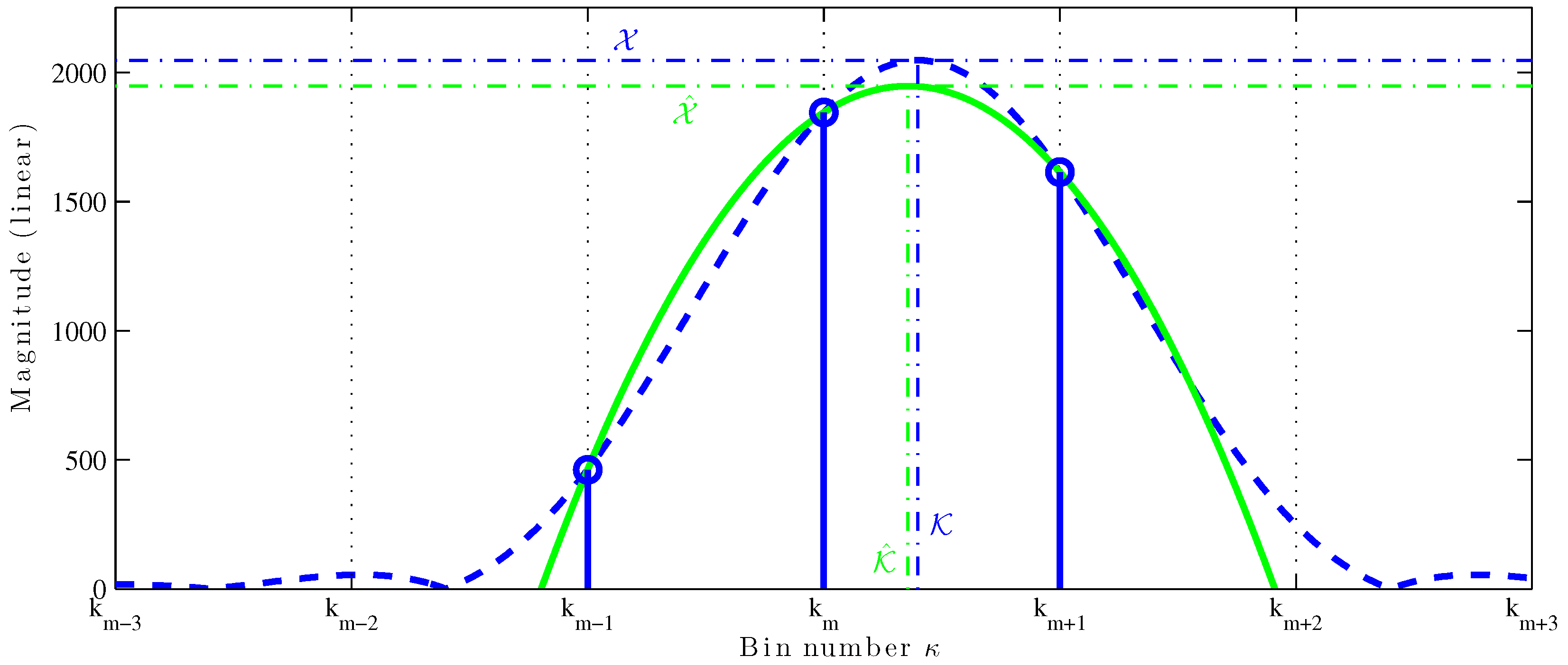
Since it is performed directly on the magnitude spectrum, we denote this technique the “magnitude-spectrum QIFFT” or MQIFFT. The parabolic fitting is shown in Figure 1. The thick dashed blue line is the DTFT of a length-4096 Hann-windowed sinusoid and the thick solid green line is a parabola fit to the top three bins ($k_{m-1}$, $k_m$, and $k_{m+1}$) of the magnitude DFT, shown as stemmed circle. The vertical dot-dashed lines mark the true fractional bin index $\mathcal{K}$ and the estimate $\widehat{\mathcal{K}}$; the horizontal dot-dashed lines mark the true amplitude $\mathcal{X}$ and the estimate $\widehat{\mathcal{X}}$. The QIFFT can be considered a perfect match to a truncated (order-2) Taylor series expansion of the window transform.

QIFFT-derived methods are very attractive, as they all have the following desirable properties: (1) they can greatly reduce estimation error; (2) they are inexpensive (requiring only a few multiplies to find the refined peak frequency and amplitude estimates); (3) they can be used with any window type with the notable exception of the non-zero-padded rectangular window as its main lobe width less that three bins [30]; and (4) they can be combined seamlessly with zero padding to further increase their accuracy.

The property of being applicable to any window type is one of the main advantages of QIFFT-derived methods. Other popular direct parameter estimation techniques are derived from properties of the rectangular window (no windowing) [2,8,18,19,36] or a particular window (e.g., [1], Cosine window) or class of windows (e.g., [16], Rife–Vincent class I windows). A few state-of-the-art methods are fully general and can be applied to any window, including methods by Duda [14] and Candan [15]. General methods have the distinct advantage of being portable to any window type, even those without analytic descriptions such as the Slepian (DPSS) window [4]. For instance, Duda gives examples of applying his method to Dolph–Chebyshev and Kaiser–Bessel windowed signals [14], which can only be approximated with Rife–Vincent class I windows and hence can’t take advantage of the approaches of, e.g., [16].

4. Proposed Method: XQIFFT

The QIFFT fits a parabola to the magnitude spectrum directly, however, it is possible to implement variations of the QIFFT where we fit parabolas to a magnitude spectrum scaled by a nonlinear function $\mathrm{f}(\Theta )=\Phi$. To qualify as a scaling, the function f needs to be invertible (and thus monotonic) with its inverse denoted as ${\mathrm{f}}^{-1}(\Phi )=\Theta$. This property is desirable for the fact that we may need to retrieve the amplitude value estimate on the original linear scale, and for the fact that this preserves the concavity property of the main lobe. These variations are based on nonlinear scalings of the magnitude spectrum estimate $(\widehat{\mathcal{K}},\widehat{\mathcal{X}})$ by:

$$\begin{array}{cc}\hfill \widehat{\mathcal{K}}& =k_m+\frac{1}{2}\frac{\mathrm{f}\left(\alpha \right)-\mathrm{f}\left(\gamma \right)}{\mathrm{f}\left(\alpha \right)-2\mathrm{f}\left(\beta \right)+\mathrm{f}\left(\gamma \right)}\hfill \end{array}$$

(13)

$$\begin{array}{cc}\hfill \widehat{\mathcal{X}}& ={\mathrm{f}}^{-1}\left(\mathrm{f}\left(\beta \right)-\frac{1}{8}\frac{{\left(\mathrm{f}\left(\alpha \right)-\mathrm{f}\left(\gamma \right)\right)}^2}{\mathrm{f}\left(\alpha \right)-2\mathrm{f}\left(\beta \right)+\mathrm{f}\left(\gamma \right)}\right).\hfill \end{array}$$

(14)

Rather than operating on α, β, and γ directly, these methods operate on nonlinear scalings $\mathrm{f}\left(\alpha \right)$, $\mathrm{f}\left(\beta \right)$, and $\mathrm{f}\left(\gamma \right)$. Since $\widehat{\mathcal{X}}$ is a linear scale estimate, we must also un-scale the vertex y-coordinate by ${\mathrm{f}}^{-1}(\Phi )$.

4.1. Logarithmically-Scaled QIFFT

A variant of the QIFFT approach is available in the literature which is calculated through a parabolic fit on a logarithmically-scaled magnitude spectrum, which we denote the “logarithmically-scaled QIFFT” or LQIFFT.

The LQIFFT uses (13) and (14) with the following nonlinear scaling and unscaling functions:

$$\begin{array}{cc}\hfill \mathrm{f}(\Theta )& =\log (\Theta )=\Phi \hfill \end{array}$$

(15)

$$\begin{array}{cc}\hfill {\mathrm{f}}^{-1}(\Phi )& =\exp (\Phi )=\Theta . \hfill \end{array}$$

(16)

The intuition leading to the use of logarithmic scaling in the QIFFT is that since the Fourier Transform (FT) of a continuous-time Gaussian window is also a Gaussian, the FT of a sinusoid will have a Gaussian-shaped main lobe. Since the logarithm of a Gaussian is exactly a parabola, using a parabolic fit on a logarithmically-scaled magnitude response of a Gaussian-windowed signal would give a perfect estimate of $(\mathcal{K},\mathcal{X})$. Considering that many popular smoothing window have a shape that can be seen as more closely approximating the shape of a Gaussian than a parabola, the logarithmic scaling was introduced in [12,31], and was shown to outperform the QIFFT on a linear scale for a variety of typical windows (Rectangular, Hann, Hamming, Blackman–Harris, Kaiser–Bessel). Note that changing the base of the logarithm has no impact on the resulting estimation—we arbitrarily choose the natural logarithm.

4.2. Power-Scaled QIFFT (XQIFFT)

While applying the QIFFT on a logarithmically-scaled magnitude spectrum was found to outperform the QIFFT on a linearly-scaled magnitude spectrum, some systematic error remains [30]. To further reduce the estimation error of the QIFFT method, we review our proposed variation on the QIFFT method that performs a parabolic fit to a magnitude spectrum rescaled by a power function [20].

The power-scaled QIFFT—the XQIFFT—uses (13) and (14) and has a tuning parameter p that controls the following nonlinear scaling and un-scaling functions:

$$\begin{array}{cc}\hfill \mathrm{f}(\Theta )& ={\Theta }^p\hfill \end{array}$$

(17)

$$\begin{array}{cc}\hfill {\mathrm{f}}^{-1}(\Phi )& ={\Phi }^{1/p}.\hfill \end{array}$$

(18)

The intuition leading to the XQIFFT is simply to try to scale the window transform shape to resemble a parabola. The performance of the XQIFFT depends heavily on choosing the tuning parameter p properly to scale the shape of the main lobe to be maximally parabolic. The shape of the main lobe is highly dependent on window type, as well as zero-padding factor and window length. Hence the proper value of p is also window-dependent. A simple procedure for choosing p is presented later, in Section 5.2.

4.3. Invariance Properties of QIFFT Methods

In this section, we show that for the XQIFFT along with the MQIFFT and LQIFFT, the estimate $\widehat{\mathcal{K}}$ is insensitive to amplitude and that the amplitude estimate $\widehat{\mathcal{X}}$ scales linearly as a function of the true amplitude $\mathcal{A}$. This property shows that the XQIFFT and its cousins are suitable for estimating sinusoids of any amplitude (other nonlinear scaling functions may not have these properties).

All the scalings discussed so far verify that the estimate in fractional bin index is insensitive to the true amplitude $\mathcal{A}$, while the estimate $\widehat{\mathcal{X}}$ scales linearly as a function of the true amplitude $\mathcal{A}$. Indeed, if we have another sinusoid of fractional bin number $\mathcal{K}$ and amplitude ${\mathcal{A}}^{\prime }=\lambda \mathcal{A}$, the QIFFT estimates (11) and (12) yield:

$$\begin{array}{cccc}\hfill {\widehat{\mathcal{K}}}^{\prime }& =k_m^{\prime }+\frac{1}{2}\frac{{\alpha }^{\prime }-{\gamma }^{\prime }}{{\alpha }^{\prime }-2{\beta }^{\prime }+{\gamma }^{\prime }}=k_m+\frac{1}{2}\frac{\lambda \alpha -\lambda \gamma }{\lambda \alpha -2\lambda \beta +\lambda \gamma }\hfill & \hfill \hspace{1em}\Rightarrow & {\widehat{\mathcal{K}}}^{\prime }=\widehat{\mathcal{K}}\hfill \end{array}$$

(19)

$$\begin{array}{cccc}\hfill {\widehat{\mathcal{X}}}^{\prime }& ={\beta }^{\prime }-\frac{1}{8}\frac{{({\alpha }^{\prime }-{\gamma }^{\prime })}^2}{{\alpha }^{\prime }-2{\beta }^{\prime }+{\gamma }^{\prime }}=\lambda \beta -\frac{1}{8}\frac{{(\lambda \alpha -\lambda \gamma )}^2}{\lambda \alpha -2\lambda \beta +\lambda \gamma }\hfill & \hfill \hspace{1em} \Rightarrow & {\widehat{\mathcal{X}}}^{\prime }=\lambda \widehat{\mathcal{X}}\hfill \end{array}$$

(20)

For the log-scaled QIFFT (13)–(16), we have the property that $\mathrm{f}(\lambda ·)=\mathrm{f}(·)+\mathrm{f}\left(\lambda \right)$, and ${\mathrm{f}}^{-1}(\mathrm{f}\left(\lambda \right)+·)$$=\lambda {\mathrm{f}}^{-1}(·)$, so that:

$$\begin{array}{cc}\hfill {\widehat{\mathcal{K}}}^{\prime }& =k_m^{\prime }+\frac{1}{2}\frac{\mathrm{f}\left({\alpha }^{\prime }\right)-\mathrm{f}\left({\gamma }^{\prime }\right)}{\mathrm{f}\left({\alpha }^{\prime }\right)-2\mathrm{f}\left({\beta }^{\prime }\right)+\mathrm{f}\left({\gamma }^{\prime }\right)}=k_m+\frac{1}{2}\frac{\mathrm{f}\left(\alpha \right)-\mathrm{f}\left(\gamma \right)}{\mathrm{f}\left(\alpha \right)-2\mathrm{f}\left(\beta \right)+\mathrm{f}\left(\gamma \right)}\Rightarrow {\widehat{\mathcal{K}}}^{\prime }=\widehat{\mathcal{K}}\hspace{1em}\hfill \end{array}$$

(21)

$$\begin{array}{cc}\hfill {\widehat{\mathcal{X}}}^{\prime }& ={\mathrm{f}}^{-1}\left(\mathrm{f}\left({\beta }^{\prime }\right)-\frac{1}{8}\frac{{\left(\mathrm{f}\left({\alpha }^{\prime }\right)-\mathrm{f}\left({\gamma }^{\prime }\right)\right)}^2}{\mathrm{f}\left({\alpha }^{\prime }\right)-2\mathrm{f}\left({\beta }^{\prime }\right)+\mathrm{f}\left({\gamma }^{\prime }\right)}\right)={\mathrm{f}}^{-1}\left(\mathrm{f}\left(\lambda \beta \right)-\frac{1}{8}\frac{{\left(\mathrm{f}\left(\alpha \right)-\mathrm{f}\left(\gamma \right)\right)}^2}{\mathrm{f}\left(\alpha \right)-2\mathrm{f}\left(\beta \right)+\mathrm{f}\left(\gamma \right)}\right)\hfill \\ & ={\mathrm{f}}^{-1}\left(\mathrm{f}\left(\lambda \right)+\mathrm{f}\left(\beta \right)-\frac{1}{8}\frac{{\left(\mathrm{f}\left(\alpha \right)-\mathrm{f}\left(\gamma \right)\right)}^2}{\mathrm{f}\left(\alpha \right)-2\mathrm{f}\left(\beta \right)+\mathrm{f}\left(\gamma \right)}\right)\Rightarrow {\widehat{\mathcal{X}}}^{\prime }=\lambda \widehat{\mathcal{X}}.\hfill \end{array}$$

(22)

For the power-scaled QIFFT (13), (14), (17) and (18), we have the property that $\mathrm{f}(\lambda ·)={\lambda }^p\mathrm{f}(·)$, and ${\mathrm{f}}^{-1}\left({\lambda }^p\mathrm{f}\left(\lambda \right)\right)=\lambda {\mathrm{f}}^{-1}(·)$, so that:

$$\begin{array}{cc}\hfill {\widehat{\mathcal{K}}}^{\prime }& =k_m^{\prime }+\frac{1}{2}\frac{\mathrm{f}\left({\alpha }^{\prime }\right)-\mathrm{f}\left({\gamma }^{\prime }\right)}{\mathrm{f}\left({\alpha }^{\prime }\right)-2\mathrm{f}\left({\beta }^{\prime }\right)+\mathrm{f}\left({\gamma }^{\prime }\right)}=k_m+\frac{1}{2}\frac{{\lambda }^p\mathrm{f}\left(\alpha \right)-{\lambda }^p\mathrm{f}\left(\gamma \right)}{{\lambda }^p\mathrm{f}\left(\alpha \right)-2{\lambda }^p\mathrm{f}\left(\beta \right)+{\lambda }^p\mathrm{f}\left(\gamma \right)}\Rightarrow {\widehat{\mathcal{K}}}^{\prime }=\widehat{\mathcal{K}}\hfill \end{array}$$

(23)

$$\begin{array}{cc}\hfill {\widehat{\mathcal{X}}}^{\prime }& ={\mathrm{f}}^{-1}\left(\mathrm{f}\left({\beta }^{\prime }\right)-\frac{1}{8}\frac{{\left(\mathrm{f}\left({\alpha }^{\prime }\right)-\mathrm{f}\left({\gamma }^{\prime }\right)\right)}^2}{\mathrm{f}\left({\alpha }^{\prime }\right)-2\mathrm{f}\left({\beta }^{\prime }\right)+\mathrm{f}\left({\gamma }^{\prime }\right)}\right)={\mathrm{f}}^{-1}\left({\lambda }^p\mathrm{f}\left(\beta \right)-\frac{{\lambda }^{2p}}{8{\lambda }^p}\frac{{\left(\mathrm{f}\left(\alpha \right)-\mathrm{f}\left(\gamma \right)\right)}^2}{\mathrm{f}\left(\alpha \right)-2\mathrm{f}\left(\beta \right)+\mathrm{f}\left(\gamma \right)}\right)\hfill \\ & ={\mathrm{f}}^{-1}\left({\lambda }^p\left[\mathrm{f}\left(\beta \right)-\frac{1}{8}\frac{{\left(\mathrm{f}\left(\alpha \right)-\mathrm{f}\left(\gamma \right)\right)}^2}{\mathrm{f}\left(\alpha \right)-2\mathrm{f}\left(\beta \right)+\mathrm{f}\left(\gamma \right)}\right]\right)\Rightarrow {\widehat{\mathcal{X}}}^{\prime }=\lambda \widehat{\mathcal{X}}.\hfill \end{array}$$

(24)

5. Estimation Error, Properties, and Reduction

In this section we provide error definitions (Section 5.1) and study interpolation bias (Section 5.2). Using these definitions, we propose a heuristic to find the optimal p value for a given windowing situation (Section 5.3). Finally, we mention correction functions which can unbias remaining systematic error (Section 5.4) and noise sensitivity properties (Section 5.5).

5.1. Error Definition

Following the error definition in [31], we compute the error in a particular fractional bin index $e_{\mathcal{K}}\left(\mathcal{K}\right)$ and a particular magnitude estimate $e_{\mathcal{X}}\left(\mathcal{K}\right)$ as follows. For each true fractional bin $\mathcal{K}$, the error in a particular fractional bin estimate is defined as

$$e_{\mathcal{K}}\left(\mathcal{K}\right)=\widehat{\mathcal{K}}-\mathcal{K}$$

(25)

and the error in a magnitude estimate is defined proportionally by

$$e_{\mathcal{X}}\left(\mathcal{K}\right)=\frac{\widehat{\mathcal{X}}-\mathcal{X}}{\mathcal{X}}.$$

(26)

Because of the invariance of $\widehat{\mathcal{K}}$ to amplitude, and the linear dependency of $\widehat{\mathcal{X}}$ to amplitude, these errors are thus independent of the true $\mathcal{X}$, so that we only need to index these by $\mathcal{K}$.

We also define the worst-case bin estimates of the fractional bin as $e_{\mathcal{K}}^{\mathrm{w}.\mathrm{c}.}$ and the magnitude as $e_{\mathcal{X}}^{\mathrm{w}.\mathrm{c}.}$, meaning the maximum errors obtained across all the possible fractional bin indices:

$$\begin{array}{cc}\hfill e_{\mathcal{K}}^{\mathrm{w}.\mathrm{c}.}& =\underset{{\Delta }_{\mathcal{K}}\in [0,\frac{1}{2}]}{\max }\left|e_{\mathcal{K}}\left({\Delta }_{\mathcal{K}}\right)\right| \hfill \end{array}$$

(27)

$$\begin{array}{cc}\hfill e_{\mathcal{X}}^{\mathrm{w}.\mathrm{c}.}& =\underset{{\Delta }_{\mathcal{K}}\in [0,\frac{1}{2}]}{\max }\left|e_{\mathcal{X}}\left({\Delta }_{\mathcal{K}}\right)\right|.\hfill \end{array}$$

(28)

These errors have means $\mathrm{E}\left[\left|e_{\mathcal{K}}\left(\mathcal{K}\right)\right|\right]$ and $\mathrm{E}\left[\left|e_{\mathcal{X}}\left(\mathcal{K}\right)\right|\right]$:

$$\begin{array}{cc}\hfill \mathrm{E}\left[\left|e_{\mathcal{K}}\left(\kappa \right)\right|\right]& =2{\int }_0^{1/2}\left|e_{\mathcal{K}}\left({\Delta }_{\kappa }\right)\right|\mathrm{d}{\Delta }_{\kappa }\hfill \end{array}$$

(29)

$$\begin{array}{cc}\hfill \mathrm{E}\left[\left|e_{\mathcal{X}}\left(\kappa \right)\right|\right]& =2{\int }_0^{1/2}\left|e_{\mathcal{X}}\left({\Delta }_{\kappa }\right)\right|\mathrm{d}{\Delta }_{\kappa }\hfill \end{array}$$

(30)

and variances $\mathrm{Var}\left(e_{\mathcal{K}}\left(\mathcal{K}\right)\right)$ and $\mathrm{Var}\left(e_{\mathcal{X}}\left(\mathcal{K}\right)\right)$.

5.2. Interpolation Bias

We know that the MQIFFT and the LQIFFT present systematic fractional bin index and amplitude errors that are strongly dependent [30] on the distance of the sinusoid’s true fractional bin index $\mathcal{K}$ from a bin center $\lfloor \mathcal{K}\rceil$. $\lfloor ·\rceil$ indicates the rounding function, which returns its argument rounded to the nearest integer. This distance, denoted by ${\Delta }_{\mathcal{K}}$, is defined as

$${\Delta }_{\mathcal{K}}=\mathcal{K}-\lfloor \mathcal{K}\rceil .$$

(31)

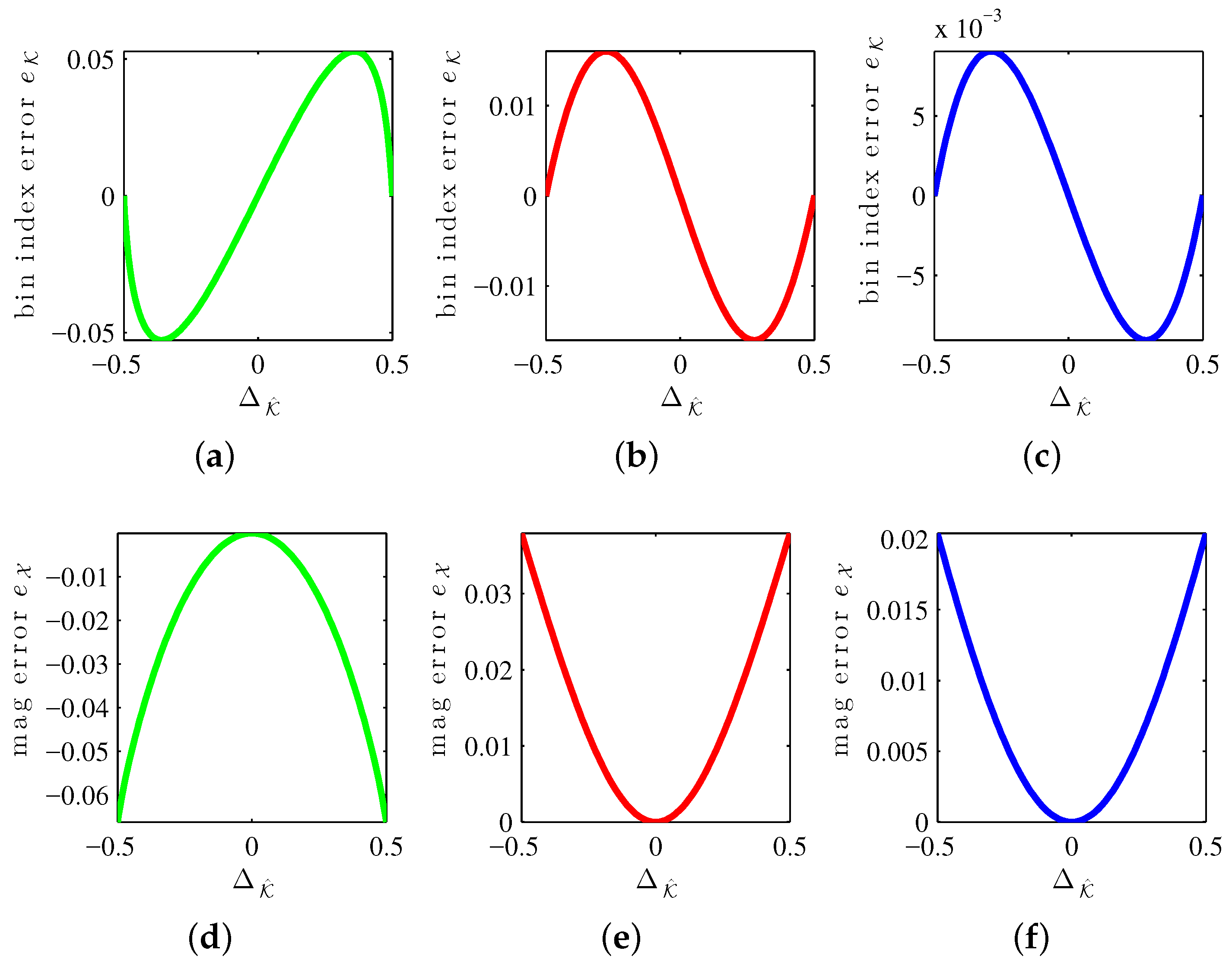
By construction, bin estimates have odd symmetry around ${\Delta }_{\mathcal{K}}=0$ and magnitude estimates have even symmetry around ${\Delta }_{\mathcal{K}}=0$ (symmetries exploited in the previous error mean and worst-case definitions). The errors in estimates associated with the XIQFFT have all these properties as well. These can be seen in the bias curves in Figure 2, which show $e_{\mathcal{K}}$ and $e_{\mathcal{X}}$ as a function of bin offset ${\Delta }_{\mathcal{K}}$ for a length-4096 Hann window.

Note that while it may sometimes (for certain windows) be possible to obtain closed form solutions for those two statistics, these solutions are generally very complex, even for simple smoothing windows. In the context of this article, we propose instead the following heuristic to evaluate those statistics numerically with arbitrary precision.

Finding the worst-case errors $e_{\mathcal{K}}^{\mathrm{w}.\mathrm{c}.}$ and $e_{\mathcal{X}}^{\mathrm{w}.\mathrm{c}.}$ requires finding the global maximum on the appropriate bias curve in Figure 2. Doing so numerically requires first to identify local maxima as the bias curves do not necessarily exhibit a single local maximum. We identify the regions containing a local maximum by computing the empirical error at a coarse sampling of the bin index space and finding the different local peaks that we associate with a single neighboring local maximum. We then run a Fibonacci search [37,38,39] (pp. 275–278, [40]) in the neighborhood of each found peak to find a local maximum. Using the Fibonacci search algorithm allows us to compute the location of that maximum up to a preset precision. We finally pick the global maximum as the largest local maximum.

Finding the mean errors $\mathrm{E}\left[\left|e_{\mathcal{K}}\left(\mathcal{K}\right)\right|\right]$ and $\mathrm{E}\left[\left|e_{\mathcal{X}}\left(\mathcal{K}\right)\right|\right]$ requires to evaluate the integral of the error function across the range of all possible bin indices (i.e., between $-0.5$ and $+0.5$). To do so numerically, we run an adaptive integration algorithm, the Simpson’s quadrature algorithm [41], on the empirical error function. This algorithm allows us to control the desired numerical precision of the final result.

For both methods, the procedure described above is aimed at obtaining estimates with arbitrary numerical precision (allowed by the Fibonacci search and the adaptive integration algorithms), while minimizing the number of empirical error function evaluations required during the extremum search (allowed by the Fibonacci search algorithm) and not requiring the derivation of a closed form error function.

5.3. Choice of the Power-Scaling Factor p

To demonstrate the XQIFFT and the process of choosing p, we study one particular representative window in detail: a length-4096 ($N=4096$) Hann window (p. 98, [42]) [43], defined as

$$w_{\mathrm{Hann}}\left(n\right)=\left[\frac{1}{2}+\frac{1}{2}\cos \left(\frac{2\pi n}{N}\right)\right].$$

(32)

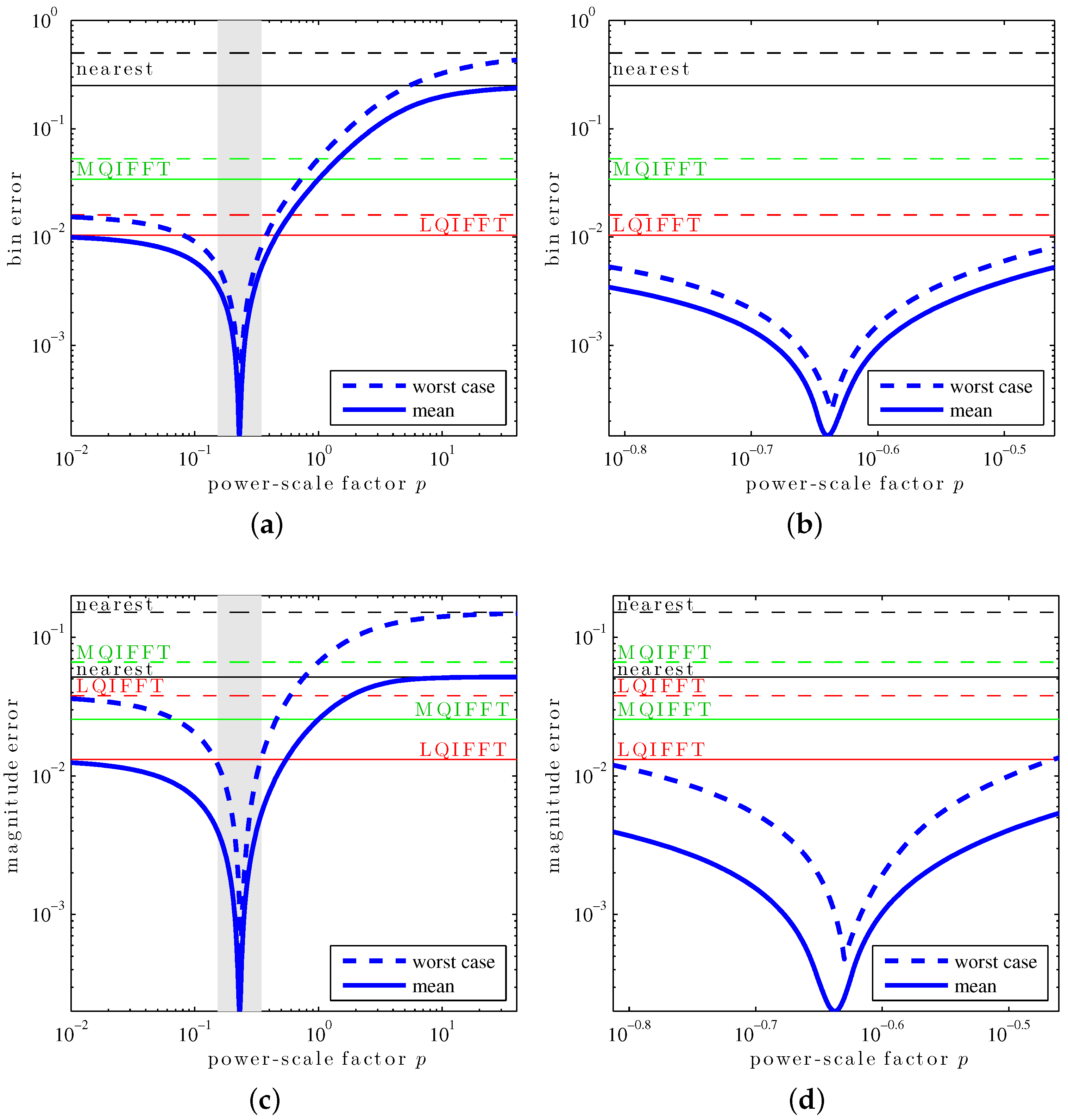
When computing the worst-case and mean errors for various values of power-scaling factor p (Figure 3), we can observe that the XQIFFT strongly outperforms the other QIFFT-derived methods if p is picked appropriately. In particular, we see that there seems to exist a single value p for which each statistic is minimized. This optimal value of p is typically different for each statistic, as well as for the chosen smoothing window, DFT length, and zero-padding factor.

As the function exhibits a single minimum (i.e., it is unimodal), we propose here to find an optimal p value numerically finding that minimum. Finding the minimum of a unimodal function can be done numerically by running a Fibonacci search on the desired error statistic. Such a heuristic yields a choice of p minimizing the desired error statistic up to an arbitrary precision order, while minimizing the number of power-scaling factors p for which we need to evaluate the statistic (using the proposed approach in Section 5.2), and still without requiring the complex derivation of a closed form solution for the different statistics as a function of p. Other estimators which allow for arbitrary windows also favor a computational rather than analytic approach [14,15].

Table 1. Comparing $e_{\mathcal{K}}\left(\mathcal{K}\right)$ and $e_{\mathcal{X}}\left(\mathcal{K}\right)$ for various estimation approaches on a length-4096 Hann window. XQIFFT cases which heuristically minimize worst case and mean error bin and magnitude errors are shown. Numbers are given to five significant figures and minimized values are shaded.

Case	${\mathit{e}}_{\mathcal{K}}^{\mathbf{w}.\mathbf{c}.}$	${\mathit{e}}_{\mathcal{X}}^{\mathbf{w}.\mathbf{c}.}$	$\mathit{E}\left[\left|{\mathit{e}}_{\mathcal{K}}\left(\mathcal{K}\right)\right|\right]$	$\mathit{E}\left[\left|{\mathit{e}}_{\mathcal{X}}\left(\mathcal{K}\right)\right|\right]$	Minimizes
nearest	5.0000 × ${10}^{-1}$	1.5110 × ${10}^{-1}$	2.5000 × ${10}^{-1}$	5.1688 × ${10}^{-2}$	n/a
MQIFFT	5.2764 × ${10}^{-2}$	6.6237 × ${10}^{-2}$	3.4221 × ${10}^{-2}$	2.5601 × ${10}^{-2}$	n/a
LQIFFT	1.5997 × ${10}^{-2}$	3.7932 × ${10}^{-1}$	1.0392 × ${10}^{-2}$	1.3121 × ${10}^{-2}$	n/a
XQIFFT, $p=0.23086$	2.4484 × ${10}^{-4}$	9.5196 × ${10}^{-4}$	1.5693 × ${10}^{-4}$	2.0239 × ${10}^{-4}$	$e_{\mathcal{K}}^{\mathrm{w}.\mathrm{c}.}$
XQIFFT, $p=0.23437$	4.4380 × ${10}^{-4}$	4.7735 × ${10}^{-4}$	2.3462 × ${10}^{-4}$	2.5251 × ${10}^{-4}$	$e_{\mathcal{X}}^{\mathrm{w}.\mathrm{c}.}$
XQIFFT, $p=0.22917$	3.1861 × ${10}^{-4}$	1.1803 × ${10}^{-3}$	1.4645 × ${10}^{-4}$	2.0637 × ${10}^{-4}$	$\mathrm{E}\left[\left|e_{\mathcal{K}}\left(\mathcal{K}\right)\right|\right]$
XQIFFT, $p=0.23039$	2.6445 × ${10}^{-4}$	1.0149 × ${10}^{-3}$	1.5203 × ${10}^{-4}$	2.0170 × ${10}^{-4}$	$\mathrm{E}\left[\left|e_{\mathcal{X}}\left(\mathcal{K}\right)\right|\right]$

shows the different error statistics from Figure 3 for the four different optimal cases. From the results, we can see that (1) for each error statistic, its associated optimal p yields an error much smaller than the MQIFFT and LQIFFT; and (2) a p value optimized for a given error statistic still yields small errors for the other ones, in particular, p values that yield small fractional bin index estimation error also yield small amplitude estimation error.

Notice that in Figure 3, the mean and worst-case bin and magnitude errors of the XQIFFT approach the performance of the nearest neighbor method for large values of p. This can be explained by the asymptotic behavior of the XQIFFT estimator as p approaches ∞. Because we have $0\le \alpha /\beta <1$ and $0\le \gamma /\beta <1$, ${\displaystyle \underset{p\to \infty }{\lim }{\left(\alpha /\beta \right)}^p=0}$ and ${\displaystyle \underset{p\to \infty }{\lim }{\left(\gamma /\beta \right)}^p=0}$ and the XQIFFT estimate (13), (14), (17) and (18) reduces to the nearest neighor method:

$$\begin{array}{cc}\hfill \widehat{\mathcal{K}}& =\underset{p\to \infty }{\lim }\left[k_m+\frac{1}{2}\frac{{\alpha }^p-{\gamma }^p}{{\alpha }^p-2{\beta }^p+{\gamma }^p}\right]=\underset{p\to \infty }{\lim }\left[k_m+\frac{1}{2}\frac{{\left(\alpha /\beta \right)}^p-{\left(\gamma /\beta \right)}^p}{{\left(\alpha /\beta \right)}^p-2+{\left(\gamma /\beta \right)}^p}\right]=k_m\hfill \end{array}$$

(33)

$$\begin{array}{cc}\hfill \widehat{\mathcal{X}}& =\underset{p\to \infty }{\lim }\left[{\left({\beta }^p-\frac{1}{8}\frac{{\left({\alpha }^p-{\gamma }^p\right)}^2}{{\alpha }^p-2{\beta }^p+{\gamma }^p}\right)}^{1/p}\right]=\underset{p\to \infty }{\lim }\left[\beta {\left(1-\frac{1}{8}\frac{{\left[{(\alpha /\beta )}^p-{(\gamma /\beta )}^p\right]}^2}{{\left(\alpha /\beta \right)}^p-2+{\left(\gamma /\beta \right)}^p}\right)}^{1/p}\right]=\beta .\hfill \end{array}$$

(34)

Additionally, we can show that, as suggested by Figure 3, the XQIFFT converges towards the LQIFFT as p approaches 0. Indeed, from the Taylor expansion of the bin estimate (13) using the XQIFFT scaling (17) and (18), we have that ${\alpha }^p=\exp \left(p\log \alpha \right)\sim 1+p\log \alpha +\mathcal{O}\left(p^2\right)$, ${\beta }^p\sim 1+p\log \beta +\mathcal{O}\left(p^2\right)$ and ${\gamma }^p\sim 1+p\log \gamma +\mathcal{O}\left(p^2\right)$. Hence, we get:

$$\begin{array}{cc}\hfill \widehat{\mathcal{K}}=\underset{p\to 0}{\lim }\left[k_m+\frac{1}{2}\frac{{\alpha }^p-{\gamma }^p}{{\alpha }^p-2{\beta }^p+{\gamma }^p}\right]& \sim \underset{p\to 0}{\lim }\left[k_m+\frac{1}{2}\frac{p\log \alpha -p\log \gamma +\mathcal{O}\left(p^2\right)}{p\log \alpha -2p\log \beta +p\log \gamma +\mathcal{O}\left(p^2\right)}\right]\hfill \\ & =k_m+\frac{1}{2}\frac{\log \alpha -\log \gamma }{\log \alpha -2\log \beta +\log \gamma }\hfill \end{array}$$

(35)

This matches (13) for a logarithmic scaling, verifying that the XQIFFT’s bin estimate (17) approaches the LQIFFT as $p\to 0$.

For the amplitude estimate (14) using the XQIFFT scaling (17) and (18) we have

$${\beta }^p-\frac{1}{8}\frac{{\left({\alpha }^p-{\gamma }^p\right)}^2}{{\alpha }^p-2{\beta }^p+{\gamma }^p}\sim 1+p\left(\log \beta +\mathcal{O}\left(p\right)-\frac{1}{8}\frac{{(\log \alpha -\log \gamma )}^2+\mathcal{O}\left(p\right)}{\log \alpha -2\log \beta +\log \gamma +\mathcal{O}\left(p\right)}\right)$$

(36)

Similarly, $\log (1+x)\sim x+\mathcal{O}\left(x^2\right)$, such that:

$$\log \left[{\beta }^p-\frac{1}{8}\frac{{\left({\alpha }^p-{\gamma }^p\right)}^2}{{\alpha }^p-2{\beta }^p+{\gamma }^p}\right]\sim p\left(\log \beta +\mathcal{O}\left(p\right)-\frac{1}{8}\frac{{(\log \alpha -\log \gamma )}^2+\mathcal{O}\left(p\right)}{\log \alpha -2\log \beta +\log \gamma +\mathcal{O}\left(p\right)}\right)+\mathcal{O}\left(p^2\right)$$

(37)

Furthermore, since ${(·)}^{1/p}=\exp \left[\frac{1}{p}\log (·)\right]$, we have:

$$\begin{array}{cc}\hfill {\left[{\beta }^p-\frac{1}{8}\frac{{\left({\alpha }^p-{\gamma }^p\right)}^2}{{\alpha }^p-2{\beta }^p+{\gamma }^p}\right]}^{1/p}& =\exp \left[\frac{1}{p}\log \left[{\beta }^p-\frac{1}{8}\frac{{\left({\alpha }^p-{\gamma }^p\right)}^2}{{\alpha }^p-2{\beta }^p+{\gamma }^p}\right]\right]\hfill \\ & \sim \exp \left[\log \beta -\frac{1}{8}\frac{{(\log \alpha -\log \gamma )}^2+\mathcal{O}\left(p\right)}{\log \alpha -2\log \beta +\log \gamma +\mathcal{O}\left(p\right)}+\mathcal{O}\left(p\right)\right]\hfill \end{array}$$

(38)

As $p\to 0$, we have $\mathcal{O}\left(p\right)\to 0$ and we then get the following limit:

$$\widehat{\mathcal{X}}=\underset{p\to 0}{\lim }\left[{\left[{\beta }^p-\frac{1}{8}\frac{{\left({\alpha }^p-{\gamma }^p\right)}^2}{{\alpha }^p-2{\beta }^p+{\gamma }^p}\right]}^{1/p}\right]=\exp \left[\log \beta -\frac{1}{8}\frac{{(\log \alpha -\log \gamma )}^2}{\log \alpha -2\log \beta +\log \gamma }\right]$$

(39)

This matches (14) for a logarithmic scaling, verifying that the XQIFFT’s amplitude estimate (18) approaches the LQIFFT as $p\to 0$.

5.4. Correction Functions

Correction functions are known to unbias some of the systematic error of interpolation on linear and logarithmic scales. Figure 4 shows systematic error curves for the MQIFFT, LQIFFT, and XQIFFT as a function of the bin estimate offset ${\Delta }_{\widehat{\mathcal{K}}}$. Similar to the bin offset (31), the bin estimate offset is defined by

$${\Delta }_{\widehat{\mathcal{K}}}=\widehat{\mathcal{K}}-\lfloor \widehat{\mathcal{K}}\rceil .$$

(40)

The reason to index the correction curves by ${\Delta }_{\widehat{\mathcal{K}}}$ instead of ${\Delta }_{\mathcal{K}}$ is that when implementing correction functions, the true value $\mathcal{K}$ (and hence ${\Delta }_{\mathcal{K}}$ which depends on it according to (31)) is not known. Only the estimate $\widehat{\mathcal{K}}$ (and hence ${\Delta }_{\widehat{\mathcal{K}}}$) is known.

Notice that all of the error curves shown in Figure 4 are highly structured. This means that it is possible to design parametric correction functions to match these curves and unbias the estimates somewhat, leading to further refinements. It should also be possible to create a tabulation of these curves when it is not convenient to develop a parametric equation. The limit of the efficacy of correction functions is controlled by the level of fitness of the fit curve or the density of a tabulation. Abe and Smith report correction functions for the LQIFFT [30] and Werner proposes magnitude and bin correction functions for the XQIFFT [20]. As we are focused solely on direct methods, a discussion of the particular form or performance of XQIFFT correction functions is outside the scope of this article since correction functions are considered to be iterative methods [27].

5.5. Sensitivity to Noise

We analyze how the parameter estimation is affected by the presence of noise in the signal. To do so we corrupt the signal $\mathcal{A}{e}^{j\left(2\pi \mathcal{F}nT+\varphi \right)}$ with different realizations of an additive white Gaussian noise random process (with zero-mean and standard deviation σ) at different levels of signal-to-noise ratio (SNR). The SNR is computed as the ratio of the amplitude of the sinusoid by the standard deviation of the noise:

$$\mathrm{SNR}=\mathcal{A}/\sigma$$

(41)

In this analysis, we quantify the effect of added noise by looking at the distribution of the noisy estimates ${\widehat{\mathcal{K}}}_G$ around the noiseless estimates $\widehat{\mathcal{K}}$. As such, we decorrelate the influence of the systematic bias associated with the estimator from the influence of the noise by reporting the bias and variance of ${\widehat{\mathcal{K}}}_G-\widehat{\mathcal{K}}$ for various bin index offsets.

In the following experiments, we consider a length-64 Hann window. We sample uniformly the bin index ${\Delta }_{\mathcal{K}}$ in $[-0.5,0]$. For each bin index, we generated ${10}^9$ noise trials to get reliable estimates of the bin index error bias and variance.

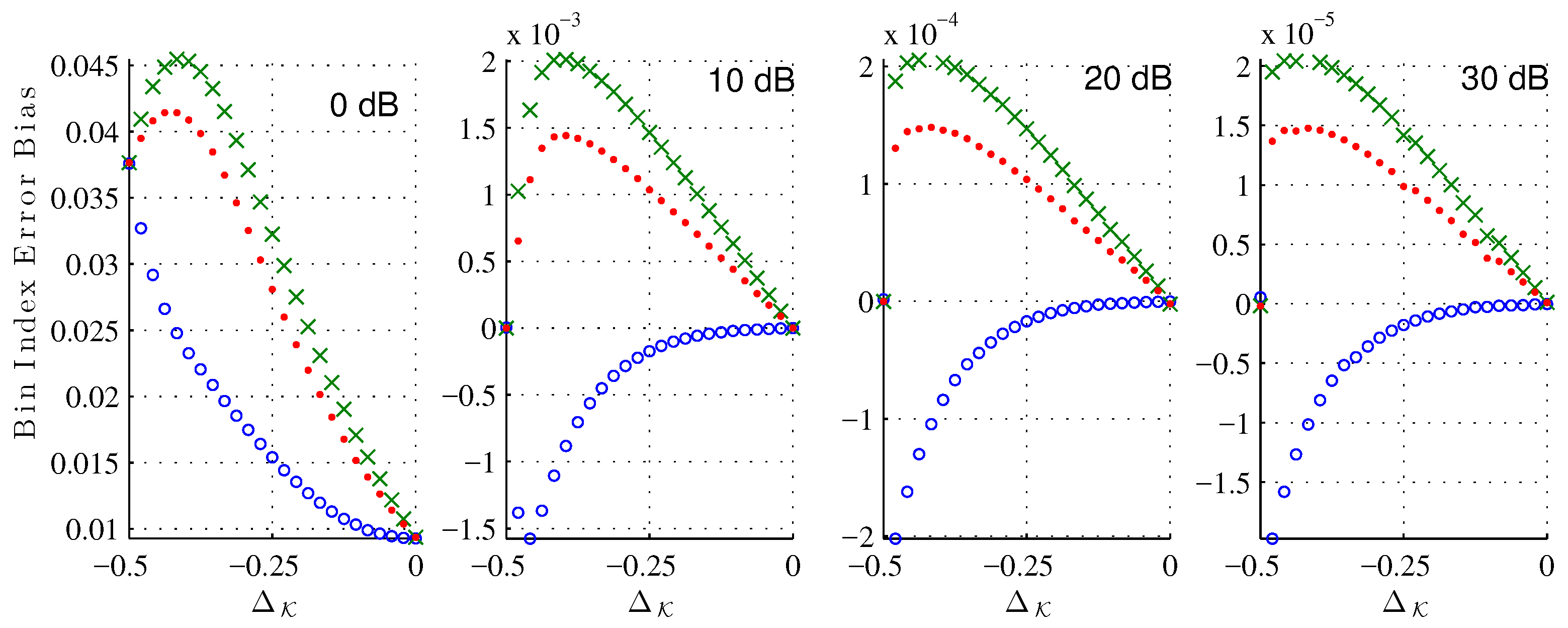
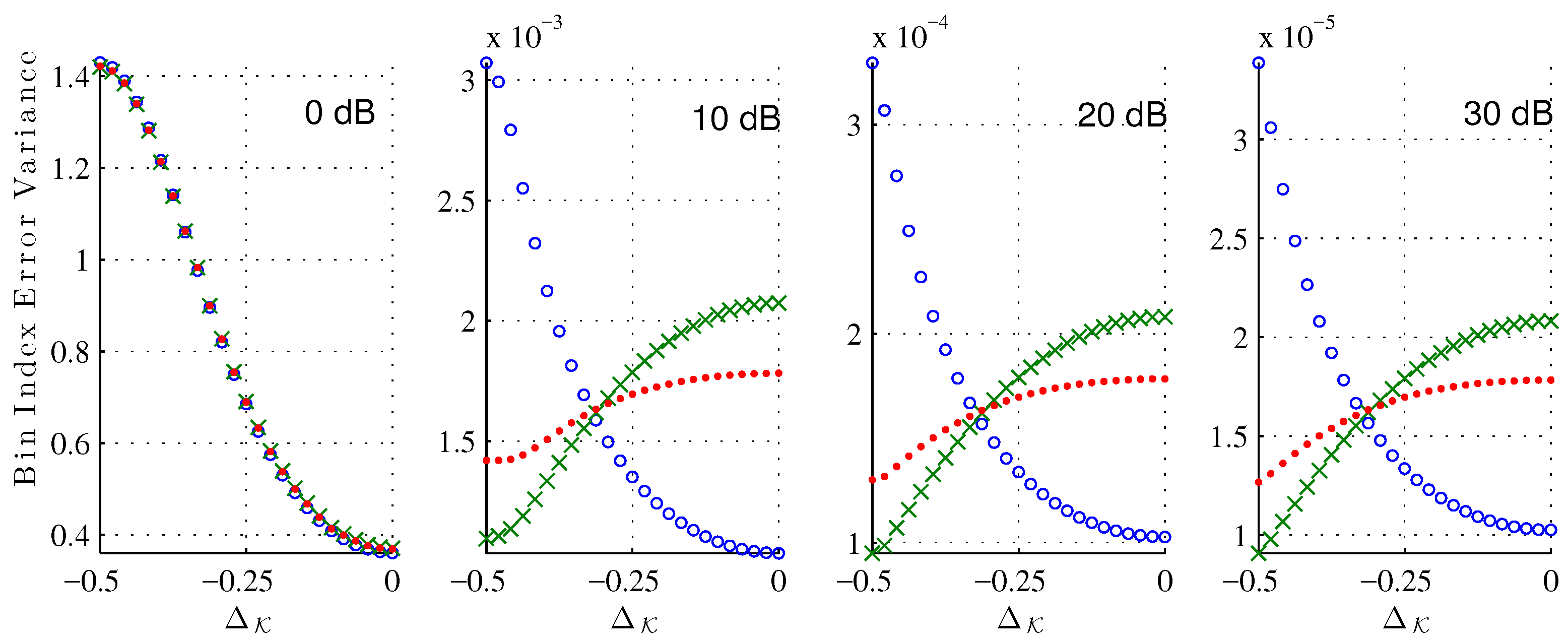
Figure 5 shows the bias of the bin index estimate (25) due to the noise corruption alone at various signal-to-noise ratios (SNR). As expected, for each estimator the bias decreases as the SNR increases. Across all ${\Delta }_{\mathcal{K}}$ and tested SNRs, the XQIFFT ($p=0.2776$) has a noise bias between that of the MQIFFT and the LQIFFT. Considering that the XQIFFT tends towards the LQIFFT as p approaches zero (as shown in Section 5.3) and is identical to the MQIFFT when $p=1$, the XQIFFT with a value of $p=0.2776$ can be considered an intermediate between the MQIFFT and LQIFFT. So, it is unsurprising that its noise bias also falls between the two. Interestingly, the bias is nonzero for most offsets ${\Delta }_{\mathcal{K}}$. This means that the presence of noise actually shifts the mean error of our estimator away from the systematic bias already present in the noiseless estimation.

Figure 6 shows the bin index error variance around the error mean. Again, the variance of the XQIFFT ($p=0.2776$) is between the MQIFFT and the LQIFFT, and we can notice that its variance has less variation across the different bin index offsets ${\Delta }_{\mathcal{K}}$.

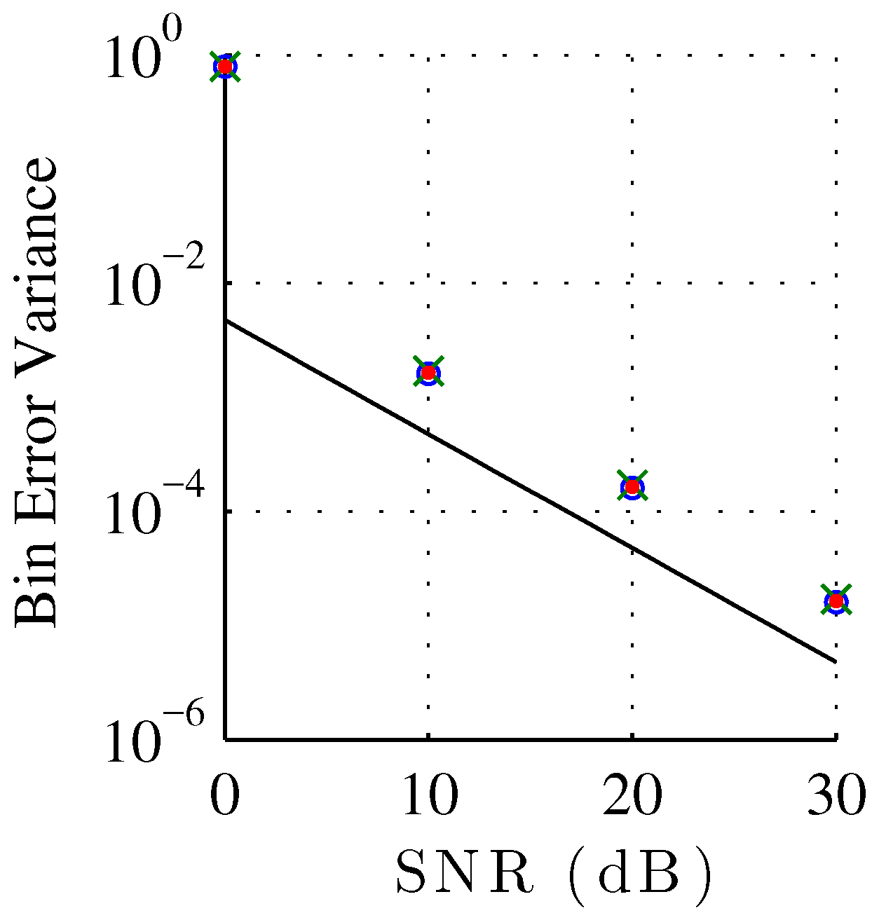
Figure 7 shows the bin index error variance of each estimator plotted against SNR, compared against the Cramér–Rao bound for unbiased estimators. Normalizing to bin width, the Cramér–Rao bound for a discrete-time signal corrupted by additive white Gaussian noise, with unknown phase and unknown amplitude is [44]

$$\mathrm{Var}\left(\widehat{\mathcal{K}}\right)=\frac{12{\sigma }^{2}N}{4{\pi }^2{\mathcal{A}}^2(N^2-1)},$$

(42)

where $N=64$ is the signal length, σ is the noise standard deviation, and $\mathcal{A}$ the sinusoid amplitude. To compare against the Cramér–Rao bound for unbiased estimation, we recompute the variance of the bin index estimation error under the assumption of a zero bias. Though we showed in Figure 5 that the estimation is not actually unbiased, the bias is commonly neglected for the noise robustness analysis of sinusoidal parameter analysis. Notice that all the QIFFT-based methods have a similar robustness against noise independently of the chosen magnitude spectrum scaling function. This result highly contrasts against the systematic estimation bias, which is highly sensitive to the choice of scaling function. We can also observe the expected thresholding effect at 0 dB [44], as the peak finding initial step becomes unreliable. The thresholding effect can also be observed in Figure 5 and Figure 6 where the behavior of the error bias and variance are very different for the 0 dB case.

From this noise sensitivity study, we can see that as long as the systematic error dominates, the best estimator will be the estimator with the lowest systematic bias—the XQIFFT with a properly-chosen value of p. At low SNR, the noise variance dominates and the methods all have a very similar compounded bias. A study on the compounded mean-squared error (MSE) comparing the XQIFFT to state-of-the-art estimators is given in the following Section.

6. Results

In this results section, the XQIFFT is compared to other QIFFT variants and two state-of-the-art estimators which, like the XQIFFT, are direct methods which can be used on any window. These two estimators are Duda’s [14] and the first step of Candan’s [15]. Candan also has a second refinement step that we do not compare to, since it corresponds to an iterative method and we are limiting our comparison to the class of direct methods.

First, we study the optimal p as a function of window length for the Hann window; Second, we study the MSE of each bin estimator for the case of a length-4096 Han window; Third, we expand that study to twelve common windows, showing that the XQIFFT minimizes MSE across all SNRs for two of the twelve tested windows.

6.1. Optimal p as a Funtion of Window Length

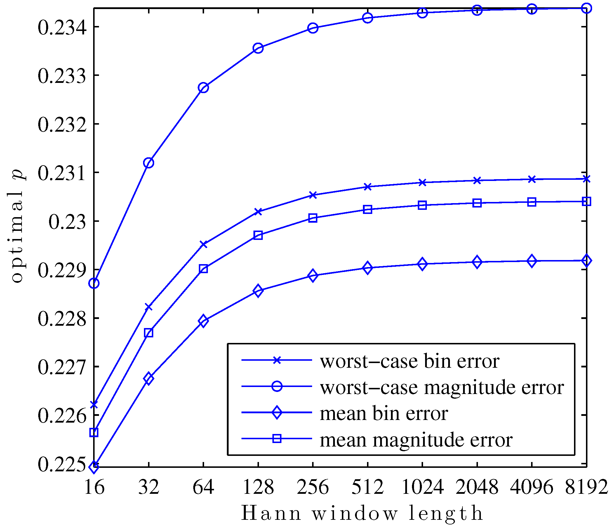
In this first study, the search for values of p which optimize $e_{\mathcal{K}}^{\mathrm{w}.\mathrm{c}.}$, $e_{\mathcal{X}}^{\mathrm{w}.\mathrm{c}.}$, $\mathrm{E}\left[\left|e_{\mathcal{K}}\left(\mathcal{K}\right)\right|\right]$, or $\mathrm{E}\left[\left|e_{\mathcal{X}}\left(\mathcal{K}\right)\right|\right]$ is repeated for Hann windows of various lengths, powers of two from 16 to 8192. The result is a family of curves, given in Figure 8, showing the optimal value of p for each window length and optimized metric.

This plot exemplifies a few interesting aspects of the search for optimal p. For any particular metric, the optimal p is a function of the shape of the main lobe within the region $\pm 1.5$ bins of its center. The reason for this is that the true DTFT peak may not be further than $\pm 0.5$ bins from a DFT bin. Since only the three closest bins are used to calculate any QIFFT-derived estimate, parts of the main lobe shape further than $\pm 1.5$ DFT bins of the DTFT peak will never be used directly in a QIFFT-derived method.

Main lobe shape is, of course, defined by the window type. A subtler but important point is that main lobe shape changes appreciably as a function of window length. This is due to the aliasing of sidelobe components of the window transform. For the Hann window, aliased sidelobe components have a decreasing effect on the main lobe shape as the window gets long due to the sidelobe rolloff of 18 dB/octave—in Figure 8 this is visible as a “flattening out” of the curves as window length increases.

Another interesting facet of this family of curves is its structure. The optimal p depends in a structured way on the window length. The same way that, e.g., Candan fits a polynomial to tabulated bias correction factors to avoid tabulating and storing every single possibility [15], it would be possible to fit a function to this family of curves to predict the optimal p for a particular metric and window shape without performing the optimization each time.

6.2. Bin Estimate MSE as a Function of SNR (Hann)

In this second study, the performance of the XQIFFT and other QIFFT-derived methods is compared to the state-of-the-art direct methods of Duda [14] and Candan [15] using again a length-4096 Hann window. Here, we choose $p=0.22917$ to minimize $\mathrm{E}\left[\left|e_{\mathcal{K}}\left(\mathcal{K}\right)\right|\right]$ as we found earlier. As before, the complex sinusoids are corrupted by additive white Gaussian noise. For each SNR from $-40$ to 120, in intervals of 5 dB, $20,000$ sinusoids are tested with bin offsets of $-0.5$ to $+0.5$. 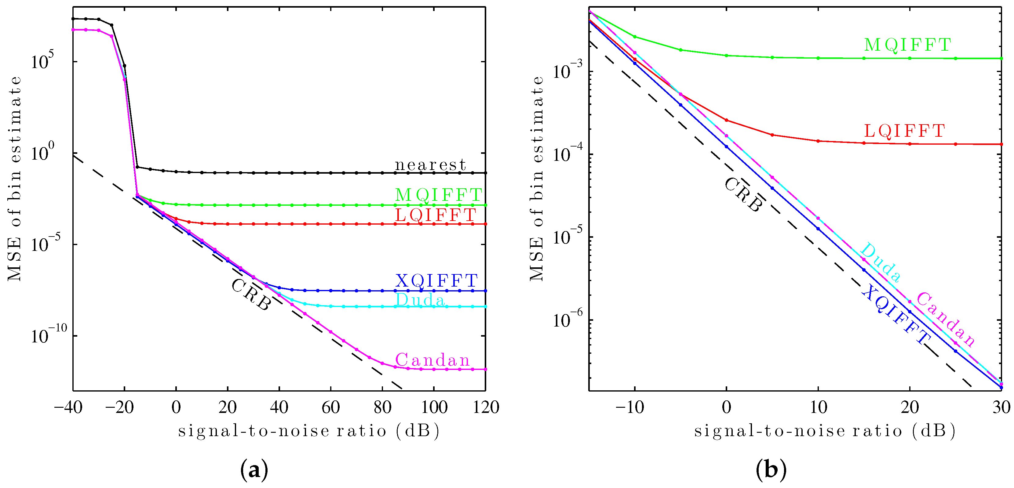The MSE of bin estimate is plotted against SNR for each method and the Cramér–Rao bound (CRB) in Figure 9a.

This plot shows a “thresholding” effect at low SNR (below $-15$ db). All of the tested methods use as their coarse estimate the maximum of the magnitude spectrum. The thresholding effect arises when the DFT samples are so noisy that the coarse estimate no longer reliably picks the DFT bin closest to the true fractional bin index $\mathcal{K}$. At low SNRs, the MSE of each method is dominated by noise—as SNR increases, the variance decreases. At high SNRs, the variance of each method is dominated by its systematic bias—noise no longer contributes much to the MSE so the traces “flatten out.”

For this particular window, the length-4096 Hann window, Figure 9a shows that Candan has the best performance at high SNRs (above 30 dB), followed by Duda, followed by the XQIFFT. However, at low SNRs (between $-15$ and 30 dB), the XQIFFT has better performance than both Duda and Candan and gets closer to the Cramér–Rao bound—a zoomed detail on this region is shown in Figure 9b.

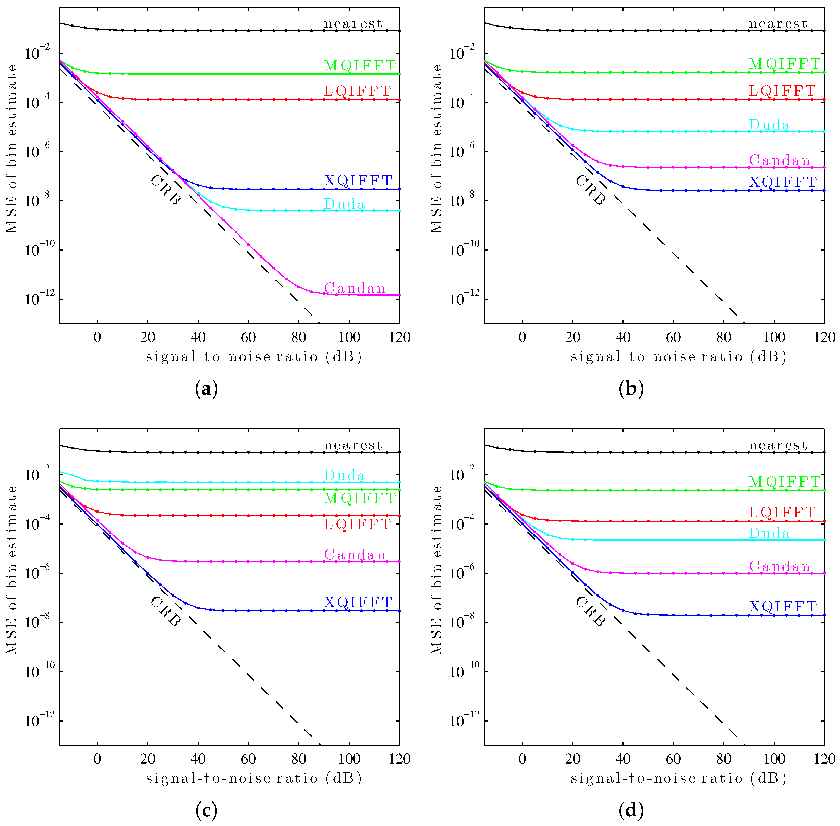
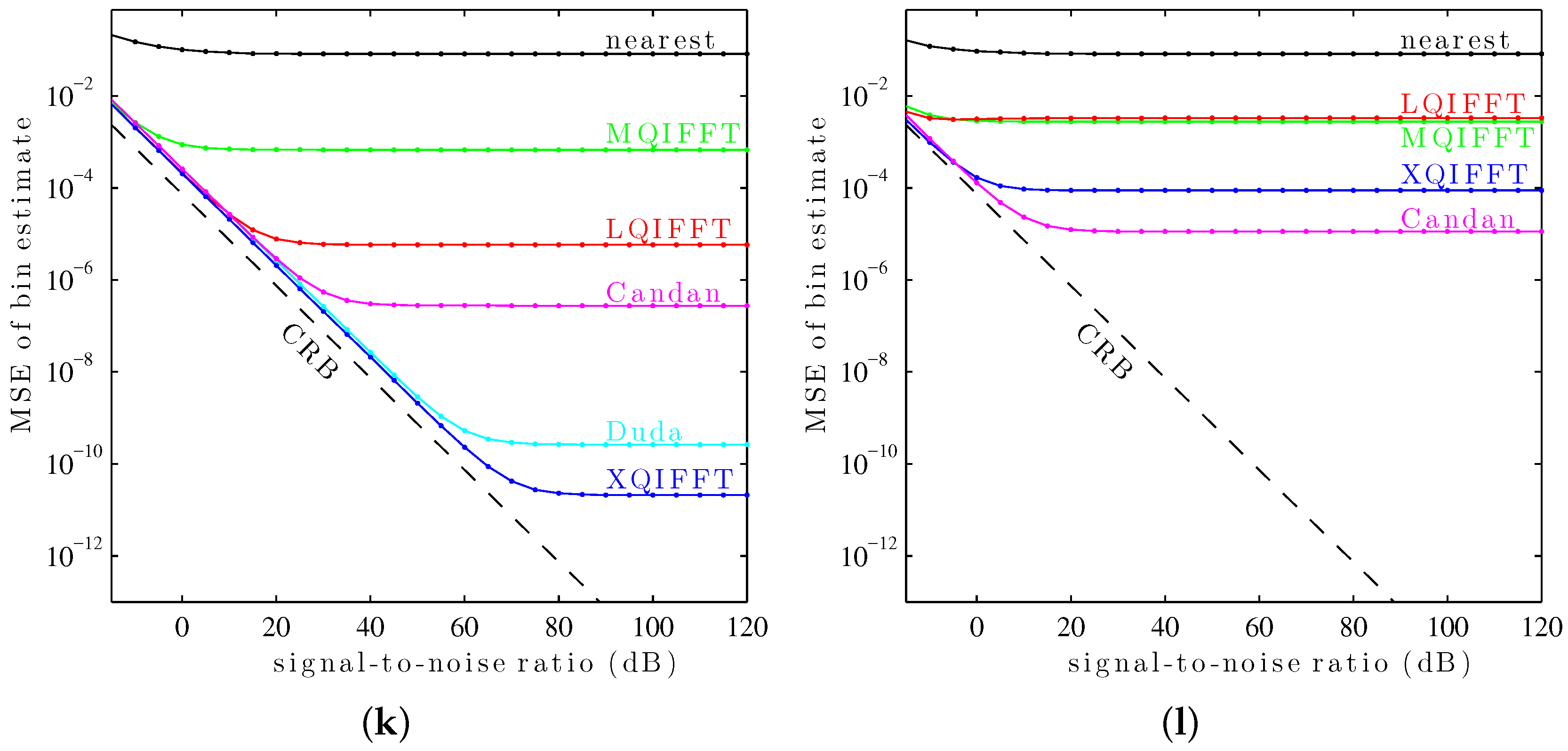
6.3. Bin Estimate MSE as a Function of SNR (Twelve Windows)

In this third study, the performance of the XQIFFT and other QIFFT-derived methods is compared to the state-of-the-art direct methods of Duda [14] and Candan [15] for twelve common length-4096 windows. These windows include the Hann window, the Bartlett–Hann window [45], the Bartlett window [4], the Hamming window [4], the Blackman window [4], the Blackman–Harris window [43], the Gaussian window [43], the Digital Prolate Spheroidal Sequence (DPSS/Slepian) window (with time–halfbandwidth product $NW=3$) [4], the Kaiser–Bessel window ($\beta =0.5$) [46], the Nuttall window [47], the Dolph–Chebyshev window (sidelobes at $-100$ dB) [43], and the Tukey window (with a 50% taper) [48]. For each of the twelve windows, p is chosen to minimize $\mathrm{E}\left[\left|e_{\mathcal{K}}\left(\mathcal{K}\right)\right|\right]$ using the procedure explained earlier. The values of p used for each window are given in

Table 2. The values of p that minimize $\mathrm{E}\left[\left|e_{\mathcal{K}}\left(\mathcal{K}\right)\right|\right]$ for the twelve length-4096 windows (highlighted column) used for tests in Figure 10, as well as length-512, -1024, and -2048 versions of the same windows. p is rounded to five decimal points.

Window	Length-512	Length-1024	Length-2048	Length-4096
Hann	$0.22903$	$0.22911$	$0.22915$	$0.22917$
Bartlett–Hann	$0.21635$	$0.21642$	$0.21645$	$0.21647$
Bartlett	$0.22530$	$0.22535$	$0.22538$	$0.22539$
Hamming	$0.18505$	$0.18575$	$0.18611$	$0.18628$
Blackman	$0.13056$	$0.13057$	$0.13058$	$0.13058$
Blackman–Harris	$0.08552$	$0.08553$	$0.08553$	$0.08554$
Gaussian	$0.12024$	$0.12074$	$0.12099$	$0.12112$
DPSS/Slepian ($NW=3$)	$0.11144$	$0.11144$	$0.11144$	$0.11144$
Kaiser–Bessel ($\beta =0.5$)	$0.28214$	$0.28270$	$0.28298$	$0.28312$
Nuttall	$0.08153$	$0.08155$	$0.08157$	$0.08157$
Dolph–Chebyshev (sidelobes at $-100$dB)	$0.08403$	$0.08403$	$0.08404$	$0.08404$
Tukey window (50% taper)	$0.50592$	$0.50609$	$0.50618$	$0.50622$

.

Again, the complex sinusoids are corrupted by additive white Gaussian noise. For each SNR from $-40$ to 120, in intervals of 5 dB, $20,000$ sinusoids are tested with bin offsets of $-0.5$ to $+0.5$. The MSE of the bin estimate is plotted against SNR for each method and the Cramér–Rao bound (CRB) in Figure 10.

It can be seen in Figure 10 that the XQIFFT (with a properly-chosen p according to Table 2) has the lowest MSE error across the entire range of SNRs for every tested window except the Hann window and the Tukey window (50% taper). In some cases the XQIFFT outperforms its closest competitor by several orders of magnitude. Figure 10 demonstrates that the XQIFFT is applicable to a wide range of common windows and that it even outperforms the state of the art for most tested windows. In a broader sense, this demonstrates that the best choice of method is highly dependent on the window type which is used—the performance ordering of different methods is highly variable, although for most windows tested the XQIFFT has the best performance. It is also interesting to note that of all the windows tested, the Nuttall window using the XQIFFT has the lowest MSE of bin estimate at high SNR. This implies that Nuttall using XQIFFT achieves the lowest systematic bias of the windows and estimators tested.

7. Conclusions

In this article, we detailed the concept of sinusoidal parameter estimation using quadratic interpolation over three bins of a power-scaled DFT surrounding a magnitude spectrum peak. This method, the XQIFFT, improves on existing quadratic interpolation methods based on linear and logarithmic scaling. We presented a heuristic for optimizing the XQIFFT power-scaling exponent p for a particular window type/window length/zero-padding factor. We presented an analysis of noise sensitivity of the proposed estimator, the dependency of the optimal exponent on window length, and a comparison with competing methods in noisy conditions under twelve common window types. We observed that across the entire tested SNR range, the proposed XQIFFT had a lower bin estimate MSE than the state-of-the-art direct estimates of Duda and Candan for ten of the twelve tested windows. From examining the high SNR regions we can also say that for ten of the twelve tested windows the XQIFFT has a lower systematic bias than the state-of-the-art methods as well. For the remaining two windows tested (Hann and Tukey), the XQIFFT has a lower MSE only at low SNR.

When implementing the XQIFFT, the reader may choose the correct value of p in one of two ways depending on their application. For common windows whose lengths are between 512 and 4096 samples, linear interpolation between the values of p reported in Table 2 may be used to approximate the optimal value of p to five decimal places. For even more precision or for window types or lengths not reported in Table 2, the reader may use the generalized procedure reported in Section 5.3 to produce an optimal value of p.

Future work should consider applying the XQIFFT-style magnitude spectrum scaling to types of estimators that rely on techniques other than parabolic interpolation. We expect that for other approaches that rely in some way on main lobe shape, the main-lobe-shaping philosophy of the XQIFFT may yield improvements.