A Cost-Effective Tracking Algorithm for Hypersonic Glide Vehicle Maneuver Based on Modified Aerodynamic Model

Abstract

In order to defend the hypersonic glide vehicle (HGV), a cost-effective single-model tracking algorithm using Cubature Kalman filter (CKF) is proposed in this paper based on modified aerodynamic model (MAM) as process equation and radar measurement model as measurement equation. In the existing aerodynamic model, the two control variables attack angle and bank angle cannot be measured by the existing radar equipment and their control laws cannot be known by defenders. To establish the process equation, the MAM for HGV tracking is proposed by using additive white noise to model the rates of change of the two control variables. For the ease of comparison several multiple model algorithms based on CKF are presented, including interacting multiple model (IMM) algorithm, adaptive grid interacting multiple model (AGIMM) algorithm and hybrid grid multiple model (HGMM) algorithm. The performances of these algorithms are compared and analyzed according to the simulation results. The simulation results indicate that the proposed tracking algorithm based on modified aerodynamic model has the best tracking performance with the best accuracy and least computational cost among all tracking algorithms in this paper. The proposed algorithm is cost-effective for HGV tracking.

1. Introduction

Hypersonic glide vehicle (HGV) [1] is a rapid strike weapon which can make long-range glide in near space by aerodynamic force at greater than Mach 5. It is a great threat to world peace that HGV can even strike anyplace in the world within two hours. Therefore, some papers about HGV tracking are published for the research of defending this weapon.

The wide range of maneuvers in three-dimension makes it really difficult to track the HGV and researchers prefer multiple model algorithms to single model algorithms for tracking the so-called strong maneuvering targets. Though the study of HGV tracking is in primary stage, there are still some representative papers about tracking some simple but not actual HGV trajectory. Zhang et al. [2] study the HGV’s Sanger trajectory [3] (without lateral maneuver) tracking using interacting multiple model (IMM) [4] algorithm based on constant acceleration (CA) model, constant turning (CT) [5] model and Singer model. Qin et al. [6] study the near space target tracking with adaptive grid interacting multiple model (AGIMM) [7] algorithm and the target trajectory is a simple combination of constant-velocity motion, constant-turning motion and constant-acceleration motion. Furthermore, the AGIMM with three different CT models is used to track the near space target, which is just called near space target but does not consist of any character of HGV. Zhai et al. [8] use adaptive IMM algorithm based on the dynamic model to study the tracking and predicting the HGV trajectory with the fixed known attack angle and the varying unknown bank angle. The attack angle and the bank angle are the two control variables. However, in real HGV trajectory tracking, the attack angle and the bank angle are unknown, which is different from all mentioned above. Thus, tracking the maneuvering trajectory with unknown attack angle and unknown bank angle will be studied in this paper using several algorithms.

If we track HGV just using some kinematic models, such as CA model, constant velocity (CV) model, CT model and so on, we may miss much important HGV information. To develop new HGV tracking algorithms using as much information as possible, in every model filter, we establish the process equation based on HGV aerodynamic model and the measurement equation according to radar measurement principle. However, the process equations of the two control variables are unknown by defenders. Hence, an effective method is needed to be proposed for modeling the rates of change of the two control variables. Furthermore, if we do not know how the two control variables change from the discrete time k-1 to k, we can also use multiple model tracking algorithms, including IMM algorithm, AGIMM algorithm and HGMM [9] algorithm. We will use different algorithms mentioned above to track the maneuvering trajectory with unknown attack angle and bank angle, and compare the accuracy and computational cost in the whole tracking stage.

Cubature Kalman filter (CKF) [10] is proposed by Arasaratnam based on the Cubature rules with rigorous mathematical derivation. CKF is more accurate than extended Kalman filter (EKF) [11] in nonlinear filter and more accurate than unscented Kalman filter (UKF) [12] in high-degree nonlinear system filter [13]. Furthermore, the system of tracking HGV is a high-degree nonlinear system. According to the above considerations, every model filter in algorithms in this paper can be constructed using CKF.

Radar is measurement equipment widely used in object detection and target tracking. In this paper, we conduct HGV tracking using only one sensor namely radar and in the future we could conduct HGV tracking using multiple sensors because of more measurement information and higher accuracy. If we used multiple sensors to measure HGV, the fuzzy multiple-sensor data fusion Kalman filter approach [14] proposed by James A. Rodger can improve the tracking performance effectively, which will be studied in the future.

This paper is organized as follows. In Section 2, the tracking algorithm based on modified aerodynamic model (MAM) is proposed, including the HGV aerodynamic model, radar measurement model and the MAM tracking algorithm. In Section 3, the multiple model tracking algorithms are proposed, including IMM tracking algorithm, AGIMM tracking algorithm and HGMM tracking algorithm. In Section 4, two typical HGV trajectories are generated and tracked using different algorithms by simulation, and the tracking performances are compared and discussed systematically. Finally, some valuable conclusions are drawn in Section 5.

2. HGV Tracking with Modified Aerodynamic Model

From above consideration, we know CKF is a good choice for high-degree nonlinear system, just like HGV tracking system. Based on CKF theory, the tracking problem of a nonlinear dynamic system can be defined by the following state-space model with additive noise in discrete time [15].

Process equation:

$$X_k=f(X_{k-1})+w_{k-1}$$

(1)

Measurement equation:

$$Y_k=h(X_k)+{\mathsf{\nu }}_{R,k}$$

(2)

where $X_k$ is the state variable at discrete time k; and $\left\{w_k\right\}$ and $\left\{{\mathsf{\nu }}_{R,k}\right\}$ are independent process and measurement Gaussian noise sequence with zero means and covariance matrixes $Q_k$ and $R_k$, respectively. Furthermore, the process equation will be established based on HGV aerodynamic model and the measurement equation will be obtained based on radar principle.

2.1. HGV Aerodynamic Model

Assuming the earth is a homogeneous sphere with rotation [16] and sideslip angle is zero, the three-dimensional point-mass dynamics of HGV in semi-speed coordinate system are described by the following equations of motion [17]:

$$\{\begin{array}{l}\frac{dV}{dt}=-D-\mathrm{gsin}\mathsf{\theta }\hfill \\ \frac{d\mathsf{\theta }}{dt}=\frac{L\cos \mathsf{\nu }}{V}+\left(\frac{V}{r}-\frac{g}{V}\right)\cos \mathsf{\theta }+2{\mathsf{\omega }}_e\cos \varphi \sin \mathsf{\sigma }\hfill \\ \frac{d\mathsf{\sigma }}{dt}=\frac{L\sin \mathsf{\nu }}{V\cos \mathsf{\theta }}+\frac{V\cos \mathsf{\theta }\sin \mathsf{\sigma }\tan \varphi }{r}-2{\mathsf{\omega }}_e\left(\cos \varphi \tan \mathsf{\theta }\cos \mathsf{\sigma }-\sin \varphi \right)\hfill \\ \frac{d\varphi }{dt}=\frac{V\cos \mathsf{\theta }\cos \mathsf{\sigma }}{r}\hfill \\ \frac{d\mathsf{\lambda }}{dt}=\frac{V\cos \mathsf{\theta }\sin \mathsf{\sigma }}{r\cos \varphi }\hfill \\ \frac{dr}{dt}=V\sin \mathsf{\theta }\hfill \end{array}$$

(3)

where $V,\mathsf{\theta },\mathsf{\sigma },r,\mathsf{\lambda }$ and $\varphi$ are the state variables, which stands for speed, flight path angle, velocity azimuth angle measured from the North in a clockwise direction, radial distance from the center of the earth to the vehicle, longitude and latitude, respectively. Bank angle $\nu$ and attack angle $\mathsf{\alpha }$ are the two unknown control variables, which will be estimated in the following sections for tracking HGV. g is gravity acceleration. t is the time. ${\mathsf{\omega }}_e$ is a coefficient related to the earth’s rotation. L and D are lift acceleration and drag acceleration, respectively, which are defined as following:

$$\{\begin{array}{l}D=\frac{C_{D}q{S}_M}{m}\\ L=\frac{C_{L}q{S}_M}{m}\end{array}$$

(4)

where $q=\frac{1}{2}\mathsf{\rho }{V}^2$ is dynamic pressure. $S_M$ is the HGV reference area. m is the HGV mass. $\mathsf{\rho }$ is mass density of air. HGV is designed based on the high-lift common aerodynamic vehicles (CAV-H) [18] so we can study the HGV aerodynamic model using the CAV-H aerodynamic parameters: m = 908 kg, $S_M= 0.484 {\mathrm{m}}^2$. Based on the U.S. Standard Atmosphere, 1976(USSA1976) [19], the mass density of air denoted as $\mathsf{\rho }$ and the sound speed a can be functions of height as

$$\mathsf{\rho }=1.225\times {10}^{-0.1133h}$$

(5)

$$a=f\left(h\right)=\{\begin{array}{c}-4.029h+340.3,h\le 10\\ -7.978\times {10}^{-4}{h}^3+0.1027h^2-2.873h+316.9,10<h\le 50\\ -1.63h+412.6,h>50\end{array}$$

(6)

where h is height in kilometers.

The drag and lift coefficient $C_D$ and $C_L$ are functions of attack angle $\mathsf{\alpha }$ and Mach number Ma, which can be expressed as:

$$\{\begin{array}{l}{C}_D=C_{D0}+C_{D1}{\alpha }^2+C_{D2}{e}^{(C_{D3}Ma)}\\ C_L=C_{L0}+C_{L1}\alpha +C_{L2}{e}^{(C_{L3}Ma)}\end{array}$$

(7)

where $C_{D0},C_{D1},C_{D2},C_{D3},C_{L0},C_{L1},C_{L2}$ and $C_{L3}$ are some fixed numerical coefficients.

Thus, we have almost established aerodynamic model. Furthermore, there are some important parameter constraints that must be considered, such as dynamic pressure q, aerodynamic load n and heat flux $\dot{Q}$. These constraints can be expressed as

$$\{\begin{array}{c}q\le q_{\max }\\ n=\frac{\sqrt{D^2+L^2}}{g}\le n_{\max }\\ \dot{Q}=K{\left(\frac{\mathsf{\rho }}{{\mathsf{\rho }}_0}\right)}^{0.5}{\left(\frac{V}{V_c}\right)}^{3.15}\le {\dot{Q}}_{\max }\end{array}$$

(8)

where $q_{\max }, n_{\max }$ and ${\dot{Q}}_{\max }$ are the maximum dynamic pressure, maximum aerodynamic load and maximum heat flux. ${\mathsf{\rho }}_0$ is the mass density of air at sea level. K is a coefficient associated with the head of HGV.

When the bank angle $\nu$ is not zero, the trajectory will maneuver laterally. Usually, in the HGV controlling, it is common to keep the attack angle fixed and keep the bank angle varying to make maneuvering laterally and skipping longitudinally trajectory. The bank angle is the main control variable and the attack angle is the auxiliary control variable for HGV controlling. Furthermore, in HGV trajectory design, the nominal attack angle is set based on engineering experience and the bank angle is used as the main control variable within the constraints of air heating, loading and dynamic pressure [20,21,22,23]. There are three main reasons for using above control approach [24]:

First, the attack angle determines the flight distance. Furthermore, once the flight mission is determined, the attack angle is determined correspondingly.

Second, the attack angle has a direct effect on aerodynamic force. The adjustments to attack angle frequently make aerodynamic force complicated, resulting in aggravating the burden of control system.

Third, the proper thermodynamic environment is provided by using big angle for HGV flight. It is harmful to the thermal protection system when adjusting attack angle frequently.

However, in some papers [17,25] the attack angle is not a constant and the two control variables can change at the same time to a large degree.

However, we will study HGV tracking using the typical trajectory with the control variables changing at the same time in this paper, which will be more convincing to validate the tracking algorithm.

Through analysis of Equations (3)–(7), we can know that the bank angle and attack angle have an important effect on flight distance. Furthermore, for an appropriate flight distance the variation ranges are usually set as follows [8]: attack angle, 6° to 12°; bank angle, −20° to 20°.

Taking the variation ranges of attack angle and bank angle into consideration, the control variables do not change at a big degree. From the aspect of kinematic models to study the trajectory HGV maneuvers strongly, but from the aspect of aerodynamic model to study the trajectory HGV does not maneuver that strongly in the long flight distance.

2.2. Radar Measurement Model

Assuming that, in the spherical coordinate system, the coordinates of the origin of the radar measurement coordinate system are ${[\begin{array}{ccc}{r}_0& {\mathsf{\lambda }}_0& {\varphi }_0\end{array}]}^T$, the coordinates of HGV centroid are ${[\begin{array}{ccc}r& \mathsf{\lambda }& \varphi \end{array}]}^T$ in the spherical coordinate system and ${\left[\begin{array}{ccc}x& y& z\end{array}\right]}^T$ in the radar measurement coordinate system. According to coordinate transforming relations, the transforming equations can be denoted as

$$\left[\begin{array}{c}r\cos \varphi \cos \mathsf{\lambda }\\ r\cos \varphi \sin \mathsf{\lambda }\\ r\sin \varphi \end{array}\right]=\left[\begin{array}{c}{r}_o\cos {\varphi }_o\cos {\mathsf{\lambda }}_o\\ r_o\cos {\varphi }_o\sin {\mathsf{\lambda }}_o\\ r_o\sin {\varphi }_o\end{array}\right]+F\left[\begin{array}{c}x\\ y\\ z\end{array}\right]$$

(9)

where F is the transform matrix of the radar measurement coordinate system to the geocentric rectangular coordinate system and can be denoted as

$$F=R_Z\left(90°-{\mathsf{\lambda }}_o\right)R_X\left(-{\varphi }_o\right)R_Y\left(90°\right)$$

(10)

where $R_Z$, $R_X$ and $R_Y$ is the rotation matrixes around the Z-axis, X-axis and Y-axis, respectively.

Assuming the HGV coordinate in radar measurement coordinate system is ${\left[\begin{array}{ccc}x& y& z\end{array}\right]}^T$, based on the radar principle [26] RAE can be expressed as:

$$\{\begin{array}{c}{R}_0=\sqrt{x^2+y^2+z^2}\\ A=\{\begin{array}{c}\arctan \left(\frac{z}{x}\right)+\mathsf{\pi },x<0\\ \arctan \left(\frac{z}{x}\right),x>0,z>0\\ \arctan \left(\frac{z}{x}\right)+2\mathsf{\pi },x>0,z<0\end{array}\\ E=\arcsin \left(y/R_0\right)\end{array}$$

(11)

In the HGV tracking, we assume the radar measurement noises are known independent white noises, so the radar measurement equations can be expressed as

$$\{\begin{array}{c}\widetilde{R_0}=R_0+{\mathsf{\epsilon }}_R\\ \tilde{A}=A+{\mathsf{\epsilon }}_A\\ \tilde{E}=E+{\mathsf{\epsilon }}_E\end{array}$$

(12)

Define $Y={[\begin{array}{ccc}\widetilde{R_0}& \tilde{A}& \tilde{E}\end{array}]}^T$ and $v_R={[\begin{array}{ccc}{\mathsf{\epsilon }}_R& {\mathsf{\epsilon }}_A& {\mathsf{\epsilon }}_E\end{array}]}^T$, then the radar measurement equation can be expressed as

$$Y=h\left(X\right)+v_R$$

(13)

The statistical characteristics of radar measurement noises $v_R$ can be expressed as

$$R=\left[\begin{array}{ccc}{\mathsf{\sigma }}_R^2& 0& 0\\ 0& {\mathsf{\sigma }}_A^2& 0\\ 0& 0& {\mathsf{\sigma }}_E^2\end{array}\right]$$

(14)

where ${\mathsf{\sigma }}_R^2$, ${\mathsf{\sigma }}_A^2$ and ${\mathsf{\sigma }}_E^2$ are measurement error deviations of range, azimuth and elevate, respectively.

2.3. Modified Aerodynamic Model Tracking Algorithm

It is known by us that the existing radar equipment cannot directly measure the attack angle and bank angle of HGV. Furthermore, the change law of the two control variables is unknown by defenders as an important secret of a strike weapon. Thus, we need to find an effective method for modeling the change law of the two control variables. Because HGV tracking is still in primary stage, there is not an existing method for modeling the change law.

To develop the MAM algorithm, we analyze the characters of HGV in near space first. HGV maneuvers by aerodynamic force with a Mach number bigger than 5 in near space and HGV can bear damage to the vehicle structure when bank angle and attack angle change strongly. Furthermore, in the practical control of HGV, the control variables usually change continuously in a certain degree for control stability. Thus, we think the rates of change of control variables in a short time are not very large and unknown by defenders.

Then, the two control variables can be modeled as constant Gaussian Markov process and we can use additive white noise to model the rates of change of attack angle and bank angle [27] as

$$\{\begin{array}{c}\frac{d\mathsf{\alpha }}{dt}=w_{t,\alpha }\approx 0\\ \frac{d\mathsf{\nu }}{dt}=w_{t,\nu }\approx 0\end{array}$$

(15)

where $w_{t,\alpha }$ and $w_{t,\nu }$ are white noise with an certain effect on attack angle and bank angle that accounts for the unknown control input.

Thus, the complete process equation can be established.

The augmented state variables at discrete time k can be defined as

$$X_k=\left[\begin{array}{cccccccc}{V}_k& {\mathsf{\theta }}_k& {\mathsf{\sigma }}_k& r_k& {\mathsf{\lambda }}_k& {\varphi }_k& {\mathsf{\alpha }}_k& {\mathsf{\nu }}_k\end{array}\right]$$

(16)

The basic process equations can be written by making Equation (3) discretization as

$$\{\begin{array}{l}{V}_{k+1}=V_k+\left(-D-g\sin {\mathsf{\theta }}_k\right)T+T{w}_{V,k}\hfill \\ {\mathsf{\theta }}_{k+1}={\mathsf{\theta }}_k+\left[\frac{L\cos {\mathsf{\nu }}_k}{V_k}+\left(\frac{V_k}{r_k}-\frac{g}{V_k}\right)\cos {\theta }_k+2{\mathsf{\omega }}_e\cos {\varphi }_k\sin {\mathsf{\sigma }}_k\right]T+T{w}_{\mathsf{\theta },k}\hfill \\ {\mathsf{\sigma }}_{k+1}={\mathsf{\sigma }}_k+\left[\frac{L\sin {\mathsf{\nu }}_k}{V_k\cos {\mathsf{\theta }}_k}+\frac{V_k\cos {\mathsf{\theta }}_k\sin {\mathsf{\sigma }}_k\tan {\varphi }_k}{r_k}-2{\mathsf{\omega }}_e\left(\cos {\varphi }_k\tan {\mathsf{\theta }}_k\cos {\mathsf{\sigma }}_k-\sin {\varphi }_k\right)\right]T+T{w}_{\mathsf{\sigma },k}\hfill \\ {\varphi }_{k+1}={\varphi }_k+\frac{V_k\cos {\mathsf{\theta }}_k\cos {\mathsf{\sigma }}_k}{r_k}T+T{w}_{\varphi ,k}\hfill \\ {\mathsf{\lambda }}_{k+1}={\mathsf{\lambda }}_k+\frac{V_k\cos {\mathsf{\theta }}_k\sin {\mathsf{\sigma }}_k}{r_k\cos {\varphi }_k}T+T{w}_{\mathsf{\lambda },k}\hfill \\ r_{k+1}=r_k+V_k\sin {\theta }_{k}T+T{w}_{r,k}\hfill \end{array}$$

(17)

Furthermore, the augmented equations about the control variables can be written by make Equation (15) discretization as

$$\{\begin{array}{c}{\mathsf{\alpha }}_{k+1}={\mathsf{\alpha }}_k+T{w}_{k,\mathsf{\alpha }}\\ {\mathsf{\nu }}_{k+1}={\mathsf{\nu }}_k+T{w}_{k,\mathsf{\nu }}\end{array}$$

(18)

where T is the time interval. $w_{V,k}$, $w_{\mathsf{\theta },k}$, $w_{\mathsf{\sigma },k}$, $w_{\varphi ,k}$, $w_{\mathsf{\lambda },k}$, $w_{r,k}$, $w_{\mathsf{\alpha },k}$ and $w_{\mathsf{\nu },k}$ are the components of $w_k$. We consider that the changes of the attack angle and the bank angle at the discrete time k and (k−1) are caused by the time interval T multiplied by white noise $w_{k-1,\mathsf{\alpha }}$ and $w_{k-1,\mathsf{\nu }}$, respectively.

The method to model the rates of change of the two control variables is similar to the method in CV model to model the rate of change of velocity [28]. In CV model the ideal equation is modified as

$$\dot{x}\left(t\right)=w\left(t\right)\approx 0$$

(19)

where the white noise $w\left(t\right)$ has a “small” effect on x that accounts for unpredictable modeling errors due to turbulence, etc.

After getting the process and measurement equations, according to CKF, we can get the predicated state ${\widehat{X}}_k$ at discrete time k using the state ${\widehat{X}}_{k-1}$ at discrete time k−1 and the new measurement $Y_k$. CKF operates only on means and covariances of the conditional densities encountered in time and measurement updates [10]. To develop this filter, a third-degree spherical-radial cubature rule is used to compute the various multi-dimensional Gaussian-weighted moment integrals. CKF provides an efficient solution even for high-dimensional nonlinear filtering problems.

3. HGV Tracking with Multiple Model Algorithms

To establish the process equation based on unmodified aerodynamic model with unknown attack angle and unknown bank angle, we can use multiple model algorithms. In the following section the three-model multiple model algorithms are established based on aerodynamic model with attack angle unmodified and bank angle modified, and the nine-model IMM algorithm is established based on unmodified aerodynamic model with both attack angle and bank angle unmodified.

Multiple model algorithms for target tracking include fixed structure multiple model (FSMM) algorithm and variable structure multiple model (VSMM) [29] algorithm. When we apply the FSMM to a complicated real system estimation, sometimes we encounter two problems [9]: First, the chosen model set may not cover the full range of the mode and the truth may lie between adjacent models. Second, even if the chosen model set is large enough to cover the full range, use of all those models does not guarantee performance improvement, not to mention the prohibitively large computational cost. To overcome those defects of FSMM estimation and increase cost-effectiveness, VSMM is proposed in [29,30,31]. IMM algorithm is one of the most popular and most cost-effective FSMM algorithms [32]. AGIMM algorithm and HGMM algorithm are two typical VSMM algorithms. Tracking algorithms using IMM algorithm, AGIMM algorithm and HGMM algorithm will be briefly showed in this section as follows.

3.1. IMM Tracking Algorithm

In this section we establish the HGV IMM tracking algorithms with three-model IMM algorithm and nine-model IMM algorithm based on aerodynamic equations and radar measurement equations. In the three-model IMM algorithm the distinguishing aerodynamic model parameters are combination of three known fixed attack angles and corresponding unknown varying bank angles. The three fixed attack angles are 6°, 9° and 12°. The process equation of corresponding unknown varying bank angle can be set as

$${\mathsf{\nu }}_k={\mathsf{\nu }}_{k-1}+T{w}_{k-1,\mathsf{\nu }}$$

(20)

In the nine-model IMM algorithm, the distinguishing aerodynamic model parameters are combination of three known fixed attack angles and three known fixed bank angles. The three known fixed bank angles are −20°, 0° and 20°. The transition between the N models is governed by a Markov chain, named as the transition probability ${\mathsf{\rho }}_{ij}$, which is selected at the beginning of the algorithm.

The IMM algorithm can be divided into four parts namely interacting, Kalman filtering (model updating), model probability calculation and estimate combination. For ease of comparison with other algorithms and considering above discussion about different nonlinear Kalman filters, we use CKF in model updating. Then, the IMM algorithm can be demonstrated as follows:

3.1.1. Interaction of the Estimates

The mixed state estimate for the CKF model $M_j$ at discrete time k−1 is calculated using outputs of the models ${\widehat{X}}_{k-1/k-1}^i$, the corresponding model probability ${\mathsf{\omega }}_{k-1}^i$, the transition probability ${\mathsf{\rho }}_{ij}$ and is given by

$${\widehat{X}}_{k-1/k-1}^{oj}={\displaystyle \sum _{i=1}^N\frac{{\mathsf{\rho }}_{ij}{\mathsf{\omega }}_{k-1}^i}{{\displaystyle \sum _{l=1}^N{\mathsf{\rho }}_{lj}{\mathsf{\omega }}_{k-1}^i}}}{\widehat{X}}_{k-1/k-1}^i$$

(21)

where N is the model number. The error covariance of the interactive state for the filter model $M_j$ at discrete time k−1 is

$$P_{k-1/k-1}^{oj}={\displaystyle \sum _{i=1}^N\left\{\frac{{\mathsf{\rho }}_{ij}{\mathsf{\omega }}_{k-1}^i}{{\displaystyle \sum _{l=1}^N{\mathsf{\rho }}_{lj}{\mathsf{\omega }}_{k-1}^i}}\left[P_{k-1/k-1}^i+\left({\widehat{X}}_{k-1/k-1}^i-{\widehat{X}}_{k-1/k-1}^{oj}\right){\left({\widehat{X}}_{k-1/k-1}^i-{\widehat{X}}_{k-1/k-1}^{oj}\right)}^T\right]\right\}}$$

(22)

where $P_{k-1/k-1}^i$ is the estimate covariance for the i-th filter at discrete time k−1.

3.1.2. Model Updating

We set ${\widehat{X}}_{k-1/k-1}^{oj}$ and $P_{k-1/k-1}^{oj}$ as the input of Cubature Kalman filter j and after once recurrence the output of Cubature Kalman filter j can be ${\widehat{X}}_{k/k}^j$ and $P_{k/k}^j$.

3.1.3. Model Probability Calculation

The likelihood of the CKF model is given by the innovation ${\tilde{Y}}_k^j$ and the covariance of the innovation $S_k^j$ from

$${\mathsf{\Lambda }}_k^j=\frac{\exp \left[-\frac{1}{2}{\left({\tilde{Y}}_k^j\right)}^T{\left(S_k^j\right)}^{-1}{\tilde{Y}}_k^j\right]}{\sqrt{{\left(2\mathsf{\pi }\right)}^M\left|S_k^j\right|}}$$

(23)

where M is the dimension of the radar measurement; ${\tilde{Y}}_k^j$ is the residual of actual measurement and prediction measurement in CKF; and $S_k^j$ is the covariance of ${\tilde{Y}}_k^j$.

The model probabilities ${\mathsf{\omega }}_k^j$ are given by Bayes rule from

$${\mathsf{\omega }}_k^j=\frac{{\mathsf{\Lambda }}_k^j{\displaystyle \sum _{i=1}^N{\mathsf{\rho }}_{ij}{\mathsf{\omega }}_{k-1}^i}}{{\displaystyle \sum _{i=1}^N{\mathsf{\Lambda }}_k^i{\mathsf{\rho }}_{ij}{\mathsf{\omega }}_{k-1}^i}}$$

(24)

3.1.4. Estimate Combination

The final output is generated by combining the state estimates from each model as

$${\widehat{X}}_{k/k}={\displaystyle \sum _{j=1}^N{\mathsf{\omega }}_k^j{\widehat{X}}_{k/k}^j}$$

(25)

$$P_{k/k}={\displaystyle \sum _{j=1}^N\left\{{\mathsf{\omega }}_k^j\left[P_{k/k}^j+\left({\widehat{X}}_{k/k}^j-{\widehat{X}}_{k/k}\right){\left({\widehat{X}}_{k/k}^j-{\widehat{X}}_{k/k}\right)}^T\right]\right\}}$$

(26)

3.2. AGIMM Tracking Algorithm

In order to solve real-world problems the use of only a small number of models is not good enough but the use of more models does not necessarily improve the performance and increases the computational burden considerably. Thus, the concept of variable structure multiple model estimation is proposed and several VSMM algorithms are developed by researchers. An effective VSMM algorithm is to make adaptive the grid of the parameters that characterize the possible modes.

In AGIMM tracking algorithm a coarse grid relating about attack angle is set up initially, and then the grid is adjusted recursively. HGV tracking using AGIMM algorithm can be demonstrated as follows:

Because the real attack angle (unknown) is assumed to be within the continuous range [6,12], we can consider a three-model IMM algorithm with time-varying supporting digraph $D_k$ and the model set $\left\{{\mathsf{\alpha }}_{1,k},{\mathsf{\alpha }}_{2,k},{\mathsf{\alpha }}_{3,k}\right\}$ for grid values (vertices of $D_k$) ${\mathsf{\alpha }}_{1,k}\le {\mathsf{\alpha }}_{2,k}\le {\mathsf{\alpha }}_{3,k}\in \left[6,12\right]$.

Initially, the AGIMM is started with the coarse grid

$$D_0=\left\{{\mathsf{\alpha }}_{1,0}=6,{\mathsf{\alpha }}_{2,0}=9,{\mathsf{\alpha }}_{3,0}=12\right\}$$

(27)

At each recursive time-step ($k\to k+1$), the grid is adjusted as following two-step adaptation logic.

3.2.1. Grid Center Readjustment

In the AGIMM algorithm, ${\alpha }_{2,k}$ is assumed to be the grid center and can be obtained by

$${\mathsf{\alpha }}_{2,k+1}{=\mathsf{\alpha }}_{1,k}{\mathsf{\omega }}_k^1{+\mathsf{\alpha }}_{2,k}{\mathsf{\omega }}_k^2{+\mathsf{\alpha }}_{3,k}{\mathsf{\omega }}_k^3$$

(28)

3.2.2. Grid Distances Readjustment

In this paper, we divide the grid distances readjustment situation into three cases no-jump, up-jump and down-jump.

Case 1.

No-jump: ${\mathsf{\omega }}_k^2$ is the biggest in ${\mathsf{\omega }}_k^1$, ${\mathsf{\omega }}_k^2$ and ${\mathsf{\omega }}_k^3$.

$${\mathsf{\alpha }}_{1,k+1}=\{\begin{array}{c}{\mathsf{\alpha }}_{2,k+1}-0.5{\mathsf{\lambda }}_{d,k},{\mathsf{\omega }}_k^1<t_1\\ {\mathsf{\alpha }}_{2,k+1}-{\mathsf{\lambda }}_{d,k},\mathrm{otherwise}\end{array}$$

(29)

$${\mathsf{\alpha }}_{3,k+1}=\{\begin{array}{c}{\mathsf{\alpha }}_{2,k+1}+0.5{\mathsf{\lambda }}_{u,k},{\mathsf{\omega }}_k^3<t_1\\ {\mathsf{\alpha }}_{2,k+1}+{\mathsf{\lambda }}_{u,k},\mathrm{otherwise}\end{array}$$

(30)

where ${\mathsf{\lambda }}_{d,k}=\max \left\{{\mathsf{\alpha }}_{2,k}-{\mathsf{\alpha }}_{1,k},\mathsf{\xi }\right\}$; ${\mathsf{\lambda }}_{u,k}=\max \left\{{\mathsf{\alpha }}_{3,k}-{\mathsf{\alpha }}_{2,k},\mathsf{\xi }\right\}$; $t_1=0.35$ is a threshold for detecting an unlikely model; and $\mathsf{\xi }=1$ is a model separation distance (design parameters).

Case 2.

Up-jump: ${\mathsf{\omega }}_k^3$ is the biggest in ${\mathsf{\omega }}_k^1$, ${\mathsf{\omega }}_k^2$ and ${\mathsf{\omega }}_k^3$.

$${\mathsf{\alpha }}_{1,k+1}={\mathsf{\alpha }}_{2,k+1}-{\mathsf{\lambda }}_{d,k}$$

(31)

$${\mathsf{\alpha }}_{3,k+1}=\{\begin{array}{c}{\mathsf{\alpha }}_{2,k+1}+2{\mathsf{\lambda }}_{u,k},{\mathsf{\omega }}_k^3>t_2\\ {\mathsf{\alpha }}_{2,k+1}+{\mathsf{\lambda }}_{u,k},\mathrm{otherwise}\end{array}$$

(32)

where $t_2=0.65$ is a threshold for detecting the significant mode.

Case 3.

Down-jump: ${\mathsf{\omega }}_k^1$ is the biggest in ${\mathsf{\omega }}_k^1$, ${\mathsf{\omega }}_k^2$ and ${\mathsf{\omega }}_k^3$

$${\mathsf{\alpha }}_{3,k+1}={\mathsf{\alpha }}_{2,k+1}{+\mathsf{\lambda }}_{u,k}$$

(33)

$${\mathsf{\alpha }}_{1,k+1}=\{\begin{array}{c}{\mathsf{\alpha }}_{2,k+1}-2{\mathsf{\lambda }}_{d,k},{\mathsf{\omega }}_k^1>t_2\\ {\mathsf{\alpha }}_{2,k+1}-{\mathsf{\lambda }}_{d,k},\mathrm{otherwise}\end{array}$$

(34)

Thus, the AGIMM algorithm for HGV tracking is defined. Through the adaptive grid method the attack angle ${\mathsf{\alpha }}_{1,k},{\mathsf{\alpha }}_{2,k}$ and ${\mathsf{\alpha }}_{3,k}$ are closer to the real unknown attack angle which is good to improve the tracking accuracy.

3.3. HGMM Tracking Algorithm

Stimulated by the idea that adding a new model set which is close to the true model will improve the performance of multiple-model estimation [33], the HGMM estimator is developed using the hybrid grid to cover a large continuous mode space with a relatively small number of models at a given accuracy level.

If the true mode is known and added to the model set, the estimator will converge to the true mode with probability 1, and the optimal state estimate can be obtained [34]. However, the true model is unknown actually, and a common way is to add the optimal mode estimate, which is statistically close to the true mode [35].

In HGMM algorithm the model set about attack angle is a combination of a fixed coarse grid and an adaptive fine grid. Denote by $A_k$ the adaptive fine grid and by M the fixed coarse subset. One cycle of HGMM algorithm consists of three steps: first, obtain the state estimate $\widehat{X}$ based on M; second, obtain the fine subset using the state estimate $\widehat{X}$; and, third, run VSMM.

Then the HGMM tracking algorithm can be demonstrated as follows:

3.3.1. Determination of the Coarse Subset

The fixed coarse grid is set as the same as that in AGIMM algorithm and can be written as

$$M=\left\{{\mathsf{\alpha }}_{1,M}=6,{\mathsf{\alpha }}_{2,M}=9,{\mathsf{\alpha }}_{3,M}=12\right\}$$

(35)

3.3.2. Determination of the Fine Subset

Two classes of approaches are presented in [36], which are simpler and easier to implement. The two approaches are: fine grid with fixed grid distance, and fine grid with adaptive grid distance. We use the first approach in this paper.

We need to get an attack angle estimate ${\widehat{\mathsf{\alpha }}}_k$ based on M using IMM algorithm and then we can form the fine grid by quantizing the region whose center is ${\widehat{\mathsf{\alpha }}}_k$ as following:

$$A_k=\left\{{\widehat{\mathsf{\alpha }}}_k-d,{\widehat{\mathsf{\alpha }}}_k,{\widehat{\mathsf{\alpha }}}_k+d\right\}$$

(36)

where d is the fixed grid distance, and in this paper we set d = 1°.

4. Simulation and Discussion

In this section, the HGV maneuvering trajectory is generated in semi-speed coordinate system and is to be measured and tracked in radar measurement coordinate system. The simulation configuration is defined in Section 4.1. The simulation results using MAM algorithm, three-model IMM algorithm, nine-model IMM algorithm, AGIMM algorithm and HGMM algorithm are compared and analyzed in Section 4.2.

4.1. Simulation Configuration

We set the initial augmented state of the HGV as follows: $V=6000$ m/s; $\theta =-0.1$ rad; $\mathsf{\sigma }=0$ rad; $r=6.378\times {10}^6+50\times {10}^3$ m; $\mathsf{\lambda }=0^{\circ }$; $\varphi =0^{\circ }$. To design a trajectory in a global strike mission, some constraints of real flight must be considered such as waypoints for reconnaissance, no-fly zones for threat avoidance, maximum dynamic pressure, maximum aerodynamic load and maximum heat flux. However, in this paper, we mainly study the HGV tracking algorithms and focus on the tracking performance of different algorithms. Thus, it is proper to design some simple but typical trajectories to test the tracking algorithms regardless of above constraints.

To validate the effectiveness of the HGV maneuvering trajectory tracking algorithms proposed in this paper, two maneuvering methods are given from

$$\{\begin{array}{l}\{\begin{array}{c}\begin{array}{c}{\mathsf{\alpha }=\mathsf{\alpha }}_{\max },V>V_1\\ \mathsf{\alpha }=\frac{{\mathsf{\alpha }}_{\max }+{\mathsf{\alpha }}_{\min }}{2}+\frac{\left({\mathsf{\alpha }}_{\max }-{\mathsf{\alpha }}_{\min }\right)\sin \left[\frac{\mathsf{\pi }\left(V-0.5\left(V_1+V_2\right)\right)}{V_1-V_2}\right]}{2},V_2<V<V_1\end{array}\\ {\mathsf{\alpha }=\mathsf{\alpha }}_{\max },V<V_2\end{array}\\ \{\begin{array}{l}\mathsf{\nu }={20}^{\circ },V>V_1\\ \mathsf{\nu }=0^{\circ },V_2<V<V_1\\ \mathsf{\nu }=-{20}^{\circ },V<V_2\end{array}\end{array}$$

(37)

$$\{\begin{array}{l}\{\begin{array}{c}\begin{array}{c}\mathsf{\alpha }={\mathsf{\alpha }}_{\max },V>V_1\\ \mathsf{\alpha }=\frac{{\mathsf{\alpha }}_{\max }+{\mathsf{\alpha }}_{\min }}{2}+\frac{\left({\alpha }_{\max }-{\alpha }_{\min }\right)\sin \left[\frac{\mathsf{\pi }\left(V-0.5\left(V_1+V_2\right)\right)}{V_1-V_2}\right]}{2},V_2<V<V_1\end{array}\\ \mathsf{\alpha }={\mathsf{\alpha }}_{\max },V<V_2\end{array}\\ \mathsf{\nu }={20}^{\circ }\sin \left(t\mathsf{\pi }/40\right)\end{array}$$

(38)

where $V_1$ = 5000 m/s, $V_2$ = 4500 m/s, ${\mathsf{\alpha }}_{\max }= {12}^{\circ }$ and ${\mathsf{\alpha }}_{\min }{= 6}^{\circ }$; t denotes the flight time. Equation (37) shows the HGV maneuvers laterally at the biggest degree. Furthermore, in the real world, controlling the bank angle cannot jump 20° immediately. The change law of Equation (37) is to challenge the tracking algorithm in simulation. Equation (38) shows the HGV maneuvers laterally by the bank angle changing in the sine law with period 80 s and amplitude 20°. Then, two HGV trajectory scenarios can be generated as Figure 1.

In Figure 1, Scenario 1 is generated based on Equation (37) and Scenario 2 is generated based on Equation (38). From Figure 1 we can know that HGV maneuvers laterally more strongly when bank angle changes according to Equation (37). Assume the radar is located at the position: $r=6.378\times {10}^6+200 \mathrm{m}$; $\mathsf{\lambda }=-\pi /32$ rad; $\varphi =\mathsf{\pi }/16$ rad. The standard deviation of the radar measurement errors is set as

$$\left[\begin{array}{ccc}{\mathsf{\sigma }}_R& {\mathsf{\sigma }}_A& {\mathsf{\sigma }}_E\end{array}\right]=\left[\begin{array}{ccc}10 \mathrm{m}& 0.5 \mathrm{mrad}& 0.5 \mathrm{mrad}\end{array}\right]$$

(39)

Every process noise covariance matrix in all tracking models is set as

$$Q=diag\left(\left[5^2,{0.001}^2,{0.001}^2,{50}^2,{0.00001}^2,{0.00001}^2,{0.01}^2,{0.01}^2\right]\right)$$

(40)

In the algorithm, simulation the time interval T is 0.1 s. The model switching probability ${\mathsf{\rho }}_{ij}$ for the multiple model algorithm is a constant matrix with a large value on the diagonal elements. The three-model switching probability can be set the same for three-model IMM, AGIMM and HGMM algorithm as

$${\mathsf{\rho }}_{ij}=\{\begin{array}{c}0.8,i=j\\ 0.1,i\ne j\end{array}$$

(41)

The nine-model switching probability for nine-model IMM algorithm can be set as

$${\mathsf{\rho }}_{ij}=\{\begin{array}{c}0.6,i=j\\ 0.05,i\ne j\end{array}$$

(42)

The initial model probability for the three-model tracking algorithm is taken assuming the second model is near to the real model of HGV; that is,

$${\mathsf{\omega }}_0^j=\{\begin{array}{c}0.6,j=2\\ 0.2,\mathrm{otherwise}\end{array}$$

(43)

The initial model probability for the nine-model tracking algorithm is taken assuming the first model is near to the real model of HGV; that is,

$${\mathsf{\omega }}_0^j=\{\begin{array}{c}0.2,j=1\\ 0.1,\mathrm{otherwise}\end{array}$$

(44)

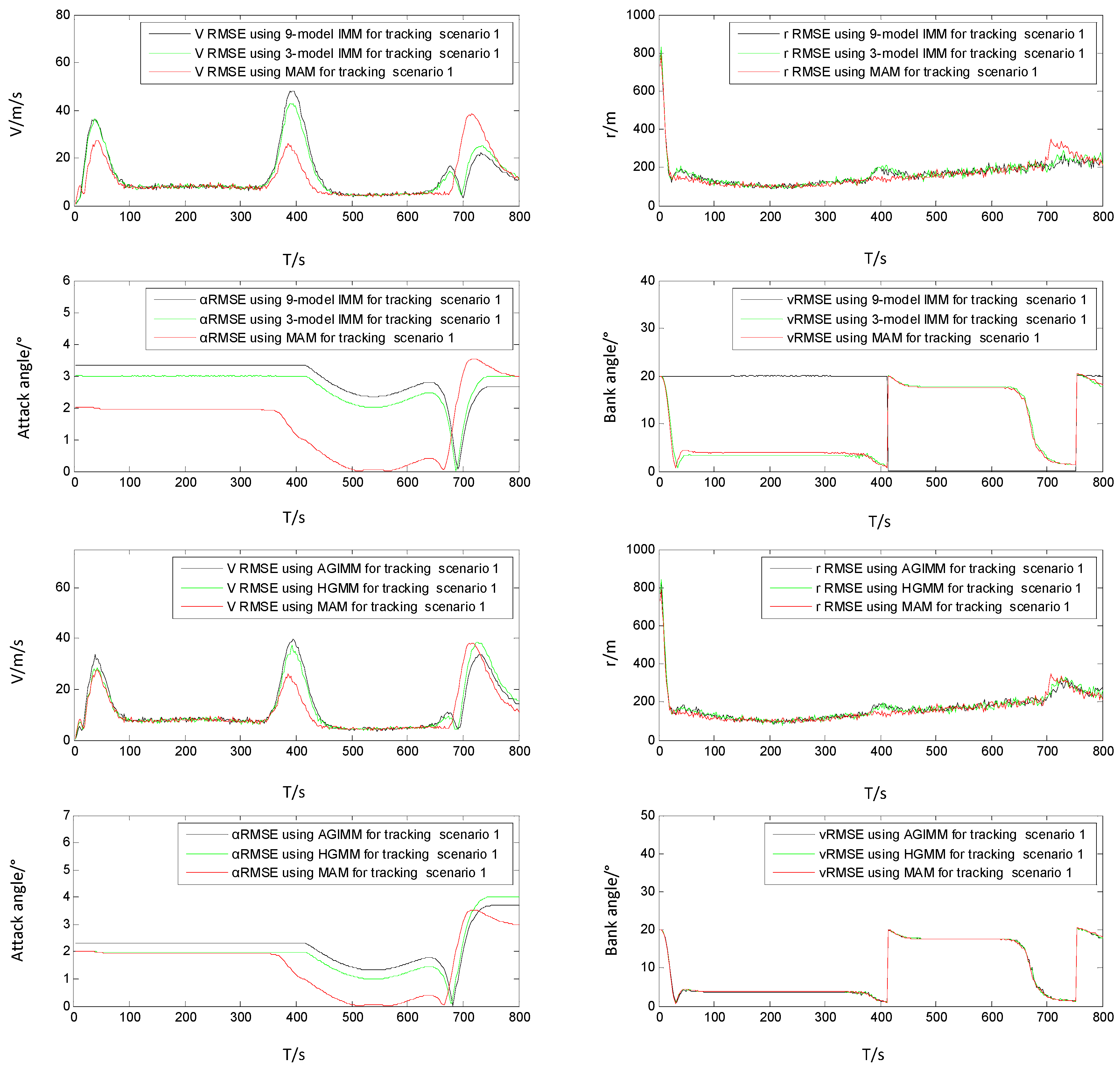
4.2. Simulation Results Comparison and Discussion

We using several different algorithms to track HGV maneuvering trajectory and run 100 Monte-Carlo simulations for every algorithm on each trajectory. We use root mean square error (RMSE) of position and velocity to compare the performances of different tracking algorithms. The RMSE, average RMSE (ARMSE) and peak RMSE (PRMSE) can be defined as

$$RMSE\left(k\right)=\sqrt{\frac{1}{n_{MC}}{\displaystyle \sum _{i=1}^{n_{MC}}{\left({\widehat{X}}_{k/k}^{(i)}-X_k\right)}^2}}$$

(45)

$$ARMSE=\frac{1}{m}{\displaystyle \sum _{k=n}^{n+m}RMSE(k)}$$

(46)

$$PRMSE=\underset{n\le k\le m+n}{\max }(RMSE(k))$$

(47)

where $n_{MC}=100$ is the Monte-Carlo simulation number; ${\widehat{X}}_{k/k}^{(i)}$ is the predicted state at discrete time k at i-th Monte-Carlo simulation; $X_k$ is the real state at discrete time k.

As defenders, velocity tracking error and position tracking error are the main indicators for HGV tracking performance [2,6,8] and more general target tracking performance [37,38,39]. Thus, in following tracking performance comparison, we mainly use velocity RMSE and position RMSE. V RMSE and r RMSE can represent the RMSE of velocity and position, respectively. Moreover, the attack angle error and bank angle error at discrete time k have a certain effect on the velocity and position at discrete time k+1. Thus, V RMSE, r RMSE, $\mathsf{\alpha }$ RMSE and $\mathsf{\nu }$ RMSE using different algorithms will be compared and analyzed as follows.

To compare the tracking performance of MAM algorithm with that of FSMM (three-model IMM and nine-model IMM) algorithm and compare the tracking performance of MAM algorithm with that of VSMM (AGIMM and HGMM) algorithm, we choose a point in every 2 s to plot the former and the later as Figure 2 for tracking Scenario 1 and as Figure 3 for tracking Scenario 2. Furthermore, the average RMSE and peak RMSE using different algorithms are listed as

Table 1. The performances for stably tracking Scenario 1.

Algorithm	V ARMSE (m/s)	V PRMSE (m/s)	r ARMSE (m)	r PRMSE (m)	$\mathsf{\alpha }$ ARMSE (°)	$\mathsf{\nu }$ ARMSE (°)
MAM	10.94	38.79	165.97	797.03	1.52	9.25
Three-model IMM	12.07	43.15	169.79	847.91	2.66	9.15
Nine-model IMM	12.27	48.61	167.27	832.13	2.91	11.49
AGIMM	12.09	40.09	172.12	862.06	2.17	9.25
HGMM	11.95	38.73	172.88	850.41	1.95	9.30

for tracking Scenario 1 and as

Table 2. The performances for stably tracking Scenario 2.

Algorithm	V ARMSE (m/s)	V PRMSE (m/s)	r ARMSE (m)	r PRMSE (m)	$\mathsf{\alpha }$ ARMSE (°)	$\mathsf{\nu }$ ARMSE (°)
MAM	10.95	38.04	161.99	790.48	1.63	14.57
Three-model IMM	12.18	40.26	164.69	842.41	2.74	14.55
Nine-model IMM	12.27	41.50	165.02	833.08	2.98	13.13
AGIMM	12.20	38.50	167.31	824.74	2.25	14.61
HGMM	12.10	39.20	168.57	863.36	2.03	14.63

for tracking Scenario 2.

From Table 1 and Table 2, we can know that the MAM algorithm outperforms multiple model algorithms in almost every ARMSE and PRMSE of velocity and position. Furthermore, VSMM algorithm performs better than FSMM algorithm for tracking Scenario 1 and Scenario 2. In VSMM algorithms, HGMM algorithm performs better than AGIMM algorithm. Although nine-model IMM algorithm uses more models, it does not perform better than three-model IMM algorithm. The tracking results using different algorithms will be analyzed and discussed in detail as follows.

Using MAM algorithm has reduced the average V RMSE by 9.36% than using three-model IMM algorithm for tracking Scenario 1, by 9.52% than using AGIMM algorithm for tracking Scenario 1, by 8.45% than using HGMM algorithm for tracking Scenario 1, by 12.18% than using three-model IMM algorithm for tracking Scenario 2, by 12.20% than using AGIMM algorithm for tracking Scenario 2, by 9.50% than using HGMM algorithm for tracking Scenario 2, respectively. Using MAM algorithm has reduced the average r RMSE by a certain degree than using other algorithms. The results that MAM (single model) algorithm outperforms other algorithms mentioned in this paper for tracking HGV trajectories contradicts the usual opinion that multiple model tracking algorithm outperforms single model (MAM) tracking algorithm for this so-called strong maneuvering target.

The HGV can make maneuver at big degree in long flight distance and maneuver strongly in three dimension from the aspect of kinematic models as Figure 1. However, the maneuver ability is not that strong as we think from the aspect of aerodynamic model because the maneuver is caused by the two control variables and the rates of change of the two control variables are not large. First, by comparing nine-model IMM algorithm with three-model IMM algorithm, we know the modeling method by Equation (20) is better cover the variation ranges of bank angle than multiple model method. Second, by comparing MAM algorithm with three-model multiple model algorithms in this paper, we know the modeling method by the equation for attack angle in Equation (19) is better to cover the variation ranges of the attack angle than the multiple model methods. Third, by comparing MAM algorithm with nine-model IMM algorithm, we known the modeling method by Equation (19) is better to cover the variation ranges of bank angle and attack angle than multiple model method. Moreover, we know from Figure 2 and Figure 3 MAM algorithm has a good attack angle and bank angle tracking performance for tracking Scenario 1 and Scenario 2. However, when tracking Scenario 2 the bank angle RMSE by nine-model IMM algorithm is lower than that by MAM algorithm. The reason is that the lateral maneuver is the position change and the position change is lagging behind acceleration change. Based on above discussion, we can know the modeling method of rates of change of the two control variables in the modified aerodynamic model for HGV tracking is better than multiple model method.

The VSMM algorithms are more efficient than FSMM algorithms as we know. In this paper, the AGIMM algorithm and HGMM algorithm perform better than IMM algorithm for HGV tracking. Furthermore, HGMM algorithm outperforms the AGIMM algorithm but has almost double computational burden. That is because that HGMM algorithm has a fixed coarse grid which covers the all possible and can overcome the mode hoping.

There is only one model filter in MAM algorithm. There are three model filters in both three-model IMM algorithm and AGIMM algorithm. There are nine model filters in nine-model IMM algorithm and six model filters in HGMM algorithm. The numbers of model filters determine mainly the computational cost of HGV tracking algorithm. Obviously, the MAM (single model) algorithm has the least computational cost. Furthermore, the MAM algorithm has the best average tracking accuracy in all these representative algorithms. Based on the above consideration, MAM algorithm is the most cost-effective algorithm for HGV tracking in those algorithms, with better accuracy and much less computational cost than other algorithms in this paper.

By comparing Table 1 with Table 2, we can know the V peak RMSE and r peak RMSE of Scenario 1 are higher than that of Scenario 2. This is because Scenario 1 maneuvers more strongly than Scenario 2 in peak points. The peak RMSE of Scenario 1 has almost the biggest lateral maneuver caused by bank angle jumping from 20° to 0° or from 0° to −20°, which means that the algorithms based on modified aerodynamic model are capable of tracking HGV effectively at good accuracy even in biggest maneuvering stage.

The simulation indicates the modified HGV aerodynamic model is effective for HGV tracking with unknown bank angle and unknown attack angle. Furthermore, the proposed method for modeling rates of changes of the control variables is more effective than multiple model methods. The tracking algorithm based on the modified aerodynamic model and radar measurement model has good tracking performance with good accuracy and little computational cost. Thus, this new proposed MAM algorithm is cost-effective for HGV tracking.

5. Conclusions

This paper mainly focuses on HGV maneuvering trajectory tracking. If we conduct HGV tracking based on kinematic models, we will miss much important information. However, we cannot conduct HGV tracking based on aerodynamic model because the attack angle and bank angle cannot be measured by existing radar equipment and the change laws of the two control variables are unknown by defenders. Thus, a modified aerodynamic model is proposed by modeling the rates of change of the two control variables with additive white noise. Based on the proposed modified aerodynamic model and radar measurement, we develop a cost-effective tracking algorithm for HGV maneuver.

We also conduct HGV tracking using multiple model algorithms, based on the unmodified aerodynamic model such as nine-model IMM algorithm and based on the half modified aerodynamic model, such as three-model IMM algorithm, AGIMM algorithm and HGMM algorithm. The tracking performances of different algorithms are compared and analyzed and simulation results indicate the MAM algorithm outperforms other multiple model algorithms, with the best accuracy and the least computational cost. The modeling method for rates of change of bank angle and attack angle is better than the multiple model method.

The proposed cost-effective tracking algorithm based on modified aerodynamic model is a good choice for HGV tracking. Because the HGV is still in experiment stage, we cannot conduct HGV tracking with real data. In the future research, we will try to develop a more effective HGV tracking algorithm and test the algorithm by tracking the real trajectory.

References

1. Li, G.; Zhang, H.; Tang, G.; Xie, Y. Maneuver modes analysis for hypersonic glide vehicles. In Proceedings of the 2014 IEEE Chinese Guidance, Navigation and Control Conference (CGNCC), Yantai, China, 8–10 August 2014; pp. 543–548.
2. Zhang, X.Y.; Wang, G.H.; Song, Z.Y.; Gu, J.J. Hypersonic sliding target tracking in near space. Def. Technol. 2015, 29, 370–381. [Google Scholar] [CrossRef]
3. Lei, M.; Han, C.Z. Expectation-maximization (EM) Algorithm Based on IMM Filtering with Adaptive Noise Covariance. Acta Autom. Sin. 2006, 32, 28–37. [Google Scholar]
4. Blom, H.A.P.; Barshalom, Y. The interacting multiple model algorithm for systems with Markovian switching coefficients. IEEE Trans. Autom. Control 1988, 33, 780–783. [Google Scholar] [CrossRef]
5. Wang, H.; Liu, G.; Gu, X. Research on Adaptive Turning Model in Grid Multiple Model Algorithm. J. Proj. Rocket. Missiles Guid. 2008, 28, 241–244. [Google Scholar]
6. Qin, L.; Li, J.; Zhou, D. Tracking filter algorithm for near space target based on AGIMM. Syst. Eng. Electron. 2015, 37, 1009–1014. [Google Scholar]
7. Jilkov, V.P. Design and comparison of mode-set adaptive IMM algorithms for maneuvering target tracking. IEEE Trans. Aerosp. Electron. Syst. 1999, 35, 343–350. [Google Scholar] [CrossRef]
8. Zhai, D.; Lei, H.; Li, J.; Liu, T. Trajectory prediction of hypersonic vehicles based on the self-adaptive IMM. Acta Aeronaut. Astronaut. Sin. 2016, 37, 245–253. [Google Scholar]
9. Xu, L.; Li, X.R.; Duan, Z. Hybrid grid multiple-model estimation with app.lication to maneuvering target tracking. IEEE Trans. Aerosp. Electron. Syst. 2016, 52, 122–136. [Google Scholar] [CrossRef]
10. Arasaratnam, I.; Haykin, S. Cubature kalman filters. IEEE Trans. Autom. Control 2009, 54, 1254–1269. [Google Scholar] [CrossRef]
11. Aidala, V.J. Kalman filter behavior in bearings-only tracking app.lications. IEEE Trans. Aerosp. Electron. Syst. 1979, AES-15, 29–39. [Google Scholar] [CrossRef]
12. Julier, S.J.; Uhlmann, J.K.; Durrant-Whyte, H.F. A new approach for filtering nonlinear systems. In Proceedings of the American Control Conference, Seattle, WA, USA, 21–23 June 1995; Volume 3, pp. 1628–1632.
13. Zhu, W.; Wang, W.; Yuan, G. An Improved Interacting Multiple Model Filtering Algorithm Based on the Cubature Kalman Filter for Maneuvering Target Tracking. Sensors 2016, 16, 805. [Google Scholar] [CrossRef] [PubMed]
14. Rodger, J.A. Toward reducing failure risk in an integrated vehicle health maintenance system: A fuzzy multi-sensor data fusion Kalman filter app.roach for IVHMS. Expert Syst. Appl. 2012, 39, 9821–9836. [Google Scholar] [CrossRef]
15. Ho, Y.-C.; Lee, R. A Bayesian approach to problems in stochastic estimation and control. IEEE Trans. Autom. Control 1964, 9, 333–339. [Google Scholar] [CrossRef]
16. Wu, N.; Chen, L. Adaptive Kalman Filtering for Trajectory Estimation of Hypersonic Glide Reentry Vehicles. Acta Aeronaut. Astronaut. Sin. 2013, 34, 1960–1971. [Google Scholar]
17. Shen, Z.; Lu, P. Dynamic lateral entry guidance logic. J. Guid. Control Dyn. 2004, 27, 949–959. [Google Scholar] [CrossRef]
18. Jorris, T.R. Common Aero Vehicle Autonomous Reentry Trajectory Optimization Satisfying Waypoint and No-Fly Zone Constraints. Ph.D. Dissertation, Air Force Institute of Technology, Dayton, OH, USA, 2007. [Google Scholar]
19. Center, N.G.D. US standard atmosphere (1976). Planet. Space Sci. 1992, 40, 553–554. [Google Scholar]
20. Li, H. Optimal design of nominal attack of angle for re-entry vehicle. J. Beijing Univ. Aeronaut. Astronaut. 2012, 38, 996–1000. [Google Scholar]
21. Wang, J. Mixed guidance method for reentry vehicles based on optimization. J. Beijing Univ. Aeronaut. Astronaut. 2010, 16, 736–740. [Google Scholar]
22. Li, H. Reentry guidance law design for RLV based on predictor-corrector method. J. Beijing Univ. Aeronaut. Astronaut. 2009, 35, 1344–1348. [Google Scholar]
23. Lu, P.; Hanson, J.M. Entry Guidance for the X-33 Vehicle. J. Spacecr. Rocket. 1998, 35, 342–349. [Google Scholar] [CrossRef]
24. Li, H. The Guidance and Control Technology for Nearspace Hypersonic Vehicle; China Astronautic Publishing House: Beijing, China, 2012. [Google Scholar]
25. Zhao, J.; Zhou, R. Reentry trajectory optimization for hypersonic vehicle satisfying complex constraints. Chin. J. Aeronaut. 2013, 26, 1544–1553. [Google Scholar] [CrossRef]
26. Ding, L.; Geng, F.; Chen, J. Radar Principle [M]; Xi’an Electronic: Xi’an, China, 1995. [Google Scholar]
27. Zhang, S.-C.; Hu, G.-D.; Liu, S.-H. Target tracking for maneuvering reentry vehicles with reduced sigma points unscented Kalman filter. In Proceedings of the 1st International Symposium on Systems and Control in Aerospace and Astronautics, Harbin, China, 19–21 January 2006.
28. Li, X.R.; Jilkov, V.P. Survey of maneuvering targettracking. Part I: Dynamic models. IEEE Trans. Aerosp. Electron. Syst. Aes 2003, 39, 1333–1364. [Google Scholar]
29. Li, X.R.; Bar-Shalom, Y. Multiple-model estimation with variable structure. IEEE Trans. Autom. Control 1996, 41, 478–493. [Google Scholar]
30. Li, X.R.; Bar-Shakm, Y. Mode-Set Adaptation in Multiple-Model Estimators for Hybrid Systems. In Proceedings of the American Control Conference, Chicago, IL, USA, 24–26 June 1992; pp. 1794–1799.
31. Li, X.R. Multiple-model estimation with variable structure: Some theoretical considerations. In Proceedings of the 33rd IEEE Conference on Decision & Control, Lake Buena Vista, FL, USA, 14–16 December 1994; pp. 1199–1204.
32. Mazor, E.; Averbuch, A.; Bar-Shalom, Y.; Dayan, J. Interacting Multiple Model Methods in Target Tracking: A Survey. IEEE Trans. Aerosp. Electron. Syst. 1998, 34, 103–123. [Google Scholar] [CrossRef]
33. Li, X.R.; Jilkov, V.P.; Ru, J. Multiple-model estimation with variable structure—Part VI: Expected-mode augmentation. IEEE Trans. Aerosp. Electron. Syst. 2005, 41, 853–867. [Google Scholar]
34. Baram, Y.; Sandell, N.R. An information theoretic app.roach to dynamical systems modeling and identification. IEEE Trans. Autom. Control 1977, 23, 1113–1118. [Google Scholar]
35. Munir, A.; Atherton, D.P. Adaptive interacting multiple model algorithm for tracking a manoeuvring target. IEE Proc. Radar Sonar Navig. 1995, 142, 11–17. [Google Scholar] [CrossRef]
36. Xu, L.; Li, X.R. Multiple model estimation by hybrid grid. Proc. Am. Control Conf. 2010, 20, 142–147. [Google Scholar]
37. Moose, R.L. An adaptive state estimation solution to the maneuvering target problem. IEEE Trans. Autom. Control 1975, AC–20, 359–362. [Google Scholar] [CrossRef]
38. Bogler, P.L. Tracking a Maneuvering Target Using Input Estimation. IEEE Trans. Aerosp. Electron. Syst. 1987, AES–23, 298–310. [Google Scholar] [CrossRef]
39. Blair, W.D.; Watson, G.A.; Rice, T.R. Tracking maneuvering targets with an interacting multiple model filter containing exponentially-correlated acceleration models. Asian J. Inf. Manag. 1991, 3, 224–228. [Google Scholar]
Figure 1. Hypersonic glide vehicle (HGV) maneuvering trajectory.
Applsci 06 00312 g001
Figure 2. Root mean square error (RMSE) for tracking Scenario 1.
Applsci 06 00312 g002
Figure 3. RMSE for tracking Scenario 2.
Applsci 06 00312 g003