Further Investigation on Laminar Forced Convection of Nanofluid Flows in a Uniformly Heated Pipe Using Direct Numerical Simulations

Abstract

In the present paper, laminar forced convection nanofluid flows in a uniformly heated horizontal tube were revisited by direct numerical simulations. Single and two-phase models were employed with constant and temperature-dependent properties. Comparisons with experimental data showed that the mixture model performs better than the single-phase model in the all cases studied. Temperature-dependent fluid properties also resulted in a better prediction of the thermal field. Particular attention was paid to the grid arrangement. The two-phase model was used then confidently to investigate the influence of the nanoparticle size on the heat and fluid flow with a particular emphasis on the sedimentation process. Four nanoparticle diameters were considered: 10, 42, 100 and 200 nm for both copper-water and alumina/water nanofluids. For the largest diameter $d_{np}=200$ nm, the Cu nanoparticles were more sedimented by around 80%, while the $A{l}_2{O}_3$ nanoparticles sedimented only by $2.5$%. Besides, it was found that increasing the Reynolds number improved the heat transfer rate, while it decreased the friction factor allowing the nanoparticles to stay more dispersed in the base fluid. The effect of nanoparticle type on the heat transfer coefficient was also investigated for six different water-based nanofluids. Results showed that the Cu-water nanofluid achieved the highest heat transfer coefficient, followed by C, $A{l}_2{O}_3$, $CuO$, $Ti{O}_2$, and $Si{O}_2$, respectively. All results were presented and discussed for four different values of the concentration in nanoparticles, namely $\mathsf{\phi }=0$, $0.6\%$, $1\%$ and $1.6\%$. Empirical correlations for the friction coefficient and the average Nusselt number were also provided summarizing all the presented results.

1. Introduction

Heat transfer is one of the most important processes in many industrial and heating-cooling applications, such as microelectronics, transportation, manufacturing, metrology, defense, and energy supply industries [1,2]. However, the inherent low thermal conductivity of conventional fluids, such as water, oils, and ethylene glycol, is a primary limitation in developing efficient heat transfer systems. The Maxwell’s theory [3] showed that an enhancement of the thermal conductivity may be achieved by dispersing millimeter or micrometer-sized solid particles into a base fluid. However one major drawback associated with the use of such large size particles is their rapid settling, which may result into a complete separation of the two phases along with the clogging of heat exchangers due to the sedimentation of the solid aggregates formed by the large size particles. This type of solid-fluid suspensions requires also the addition of a large number of particles resulting in significantly greater pressure drop, hence increased pumping power, corrosion of the walls and a noticeable increase in the wall shear stress. Thus, Choi and Eastman [4] suggested a novel approach to enhance heat transfer processes in industrial applications by exploiting the properties of nanoparticles and their dispersion in a host fluid. These metallic or non-metallic nanoparticles have an equivalent diameter $d_{np}$ lower than 100 nm. As opposed to milli- or microsized suspensions, very stable suspensions may be achieved by introducing nanoparticles. Moreover, nanoparticles benefit from a ${10}^3$ times larger surface/volume ratio than that of microparticles and exhibit much higher thermal conductivity than that of base fluids. For examples, the thermal conductivities of copper or alumina at room temperature are about 670 and 70 times greater than that of water, respectively [5]. On the contrary, it leads most of the time to a decrease in the heat capacity [6,7] and an increase in the dynamic viscosity of the mixture [6]. A compromise must be then found between the increase in thermal conductivity without loosing too much heat storage capacity and consuming too much power for pumping. If well stabilized, nanofluids represent nowadays a major technological and economical challenge and should offer very interesting perspectives for any heat transfer process.

The exponential increase in the number of publications about nanofluids [8] prevents from making an exhaustive state-of-the-art review on the topic. Many authors concentrated on measuring the thermophysical properties of various nanofluids showing that their properties depend on a large number of parameters such as the type of nanoparticle, their size, their mass or volume fraction, the type and the concentration of the surfactant, the pH of the mixture, the Brownian motion and the thickness of the interfacial nanolayer among other parameters (see in [6,7,8,9,10]). Others developed experimental set-ups to measure the convective heat transfer and temperature profiles in pipes [11,12], coaxial [13] or plate [14] heat exchangers among other geometries. Most authors focused on measuring global thermal quantities due to the difficulty to measure velocity and temperature profiles in such insulated systems. It has relatively slowed down the development of accurate models dedicated to nanofluid flows, especially regarding the agglomeration and sedimentation processes.

Only a few in-house solvers have been developed to investigate convective nanofluid flows. Most of them assume the flow as being a single-phase flow with constant or variable nanofluid properties in canonical configurations. For example, Mehrez et al. [15] numerically investigated the entropy generation and the mixed convection heat transfer of copper/water-based nanofluids in an inclined open cavity with uniform heat flux at the wall. During the last decade, many other authors compared the performance of the different single and two-phase models with constant or temperature-dependent properties in the context of nanofluid flows [16,17,18,19,20,21]. A detailed state-of-the-art review has been besides recently proposed by Kakaç and Pramuanjaroenkij [10]. Bianco et al. [17] compared the predictions of single and two-phase models (discrete phase model) with constant or temperature-dependent properties for a laminar forced convection flow of $A{l}_2{O}_3$/water-based nanofluids. They concluded that models with temperature-dependent properties lead to higher values of the heat transfer coefficient and Nusselt number, while decreasing the wall shear stress. With variable properties and for a volume fraction of $A{l}_2{O}_3$ nanoparticles equal to $4\%$, similar results have been found using single- and two-phase models with a maximum difference of $11\%$. On the contrary, Lotfi et al. [18] showed that the mixture model performs better than the single-phase model and the Eulerian one. Akbari et al. [19] compared three different two-phase models and a single-phase model to the experiments of Wen and Ding [11] for $A{l}_2{O}_3$/water-based nanofluids. The mixture, Volume of Fluid (VOF) and Eulerian models provided very similar results for the thermal field, while the single-phase model strongly underestimated the heat transfer coefficient. No clear consensus arises then from these former studies on the choice of the appropriate single- or two-phase flow models. Some attempts have also been achieved to investigate the influence of constant or variable thermophysical properties on the performances of single-phase flow models. In that, Labonté et al. [16] showed that the model with constant properties tends to underestimate the wall shear stress and overestimate the heat transfer coefficient. Azari et al. [20] found that the single-phase model with constant physical properties provides an acceptable agreement with the experimental data and the temperature-dependent model improves the predictions of the discrete two-phase flow model for low volume fractions in nanoparticles, typically $\mathsf{\phi }=0.03\%$. On the contrary, at higher particle concentrations $\mathsf{\phi }=3.5\%$, the two-phase flow performs best. Numerical modeling of laminar convective nanofluid flows even in relatively simple geometries remains very challenging, since the choice of the single- or two-phase flow models appears to be very case dependent.

Analytical models have also been developed to investigate the entropy generation in similar configurations. For example, one could cite the recent work of Bianco et al. [22], who investigated the entropy generation of $A{l}_2{O}_3$-water nanofluid turbulent forced convection in a pipe with constant wall temperature by means of a second law analysis. They showed in particular that the type of inlet conditions greatly influences the mechanisms responsible for entropy generation. Such analysis could be then very helpful to optimize nanofluid flows from an exergetic point of view.

The present paper focuses on the convective heat transfer in a cylindrical pipe for laminar flows of $A{l}_2{O}_3$/water-based nanofluids. This choice is justified by the large number of former works using this nanofluid in a similar flow configuration (laminar or developing flows in a pipe with constant heat flux) [23,24]. Moreover, such nanofluid is of a particular interest due to its non-corrosive properties and its good thermal conductivity enhancement using very low volume fractions in nanoparticles. For examples, Wang and Li [25] obtained an enhancement of $13\%$ using only a volume fraction equal to $0.4\%$ and Liu et al. [26] measured an increase of $34\%$ for a nanoparticle diameter equal to 33 nm and a volume fraction of $3\%$. The reader can refer to the reviews by Kakaç and Pramuanjaroenkij [10,27] for more details about the thermal enhancement using nanofluids.

The objective of the present paper is four-fold: (1) to properly revisit the laminar forced convection flows of $A{l}_2{O}_3$/water-based nanofluids using direct numerical simulations; (2) to extend the results to a wider range of Reynolds numbers as proposed by [19]; (3) to quantify the influence of the nanoparticle diameter and the type of nanoparticle on the hydrodynamic and thermal fields with an emphasis on the sedimentation process; (4) to provide useful empirical correlations for the friction coefficient and average Nusselt number. The experimental set-up developed by Wen and Ding [11] and the former numerical simulations of Akbari et al. [19] using the same model have been chosen for comparisons in the case of $A{l}_2{O}_3$/water-based nanofluids with the present simulations. The paper is then organized as follows: the numerical modeling and its validation are presented in Section 2 and Section 3 respectively. The influence of the Reynolds number, the concentration in nanoparticles, their diameter and the type of nanoparticles on the heat transfer process and the hydrodynamic field are then discussed in details in Section 4, before some concluding remarks in Section 5.

2. Numerical Approach

Three-dimensional calculations are carried out in the case of forced convection nanofluid flows in a heated pipe. Single- and two-phase flow models are both considered with constant or temperature-dependent properties using a finite-volume solver.

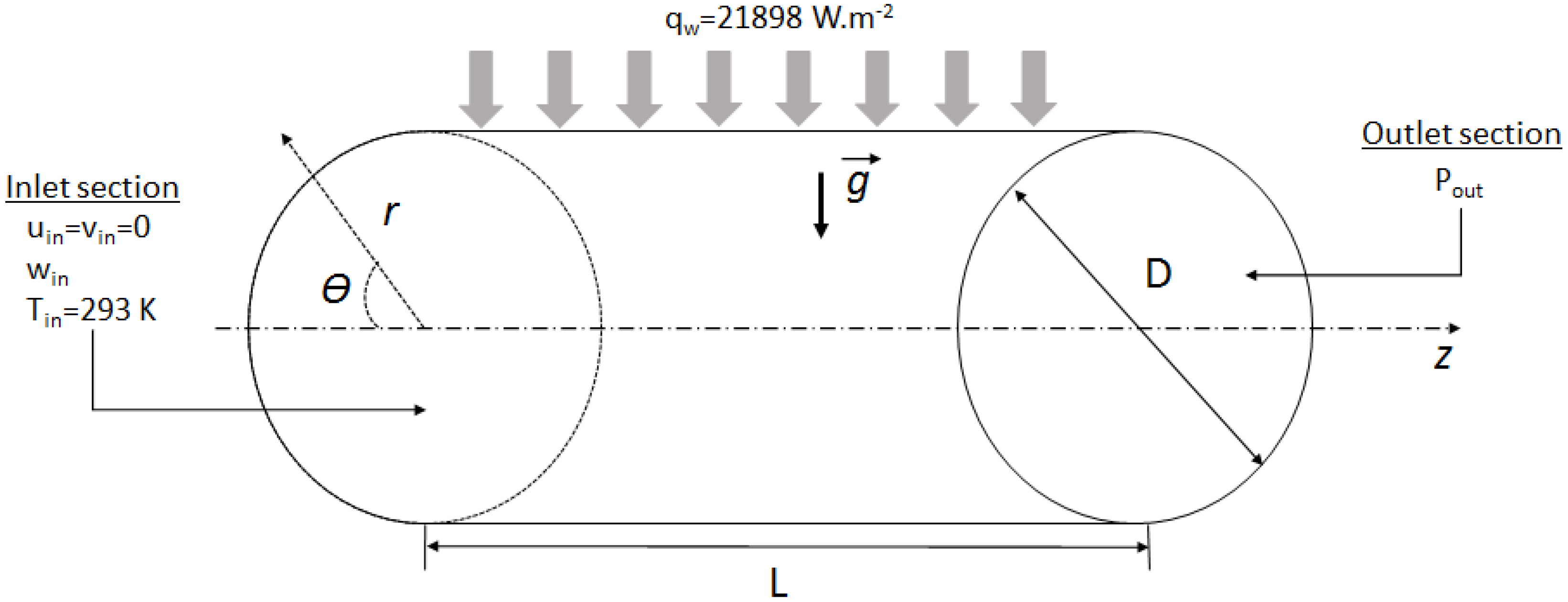
2.1. Geometrical Modeling

The problem under consideration involves nanoparticles of diameter $d_{np}$ perfectly monodispersed in pure liquid water. The geometry corresponds to the experimental set-up developed by Wen and Ding [11]. It consists of a horizontal cylindrical pipe of a length $L=0.97$ m and a diameter $D=2R=0.0045$ m, heated with a uniform heat flux $q_w=21898$ W·m${}^{-2}$ along the wall (Figure 1).

2.2. Numerical Method

The governing equations for the conservation of mass, momentum and energy are solved using a finite volume solver in a Cartesian frame. These equations are discretized in space by a second-order upwind scheme. The pressure-velocity coupling is achieved using the SIMPLEC algorithm. All calculations are performed in steady-state. It has been carefully checked that unsteady calculations led to similar results.

2.3. Fluid Properties and Two-Phase Modeling

2.3.1. Water Properties

The physical properties of water are considered to be temperature-dependent while those of the solid nanoparticles are kept constant (see

Table 1. Thermophysical properties of different types of nanoparticles.

	$\mathsf{\rho }$ (kg·m${}^{-3}$)	${\mathit{C}}_{\mathit{p}}$ (J·kg${}^{-1}$·K${}^{-1}$)	k (W·m${}^{-2}$·K${}^{-1}$)
C	220	710	129
$Cu$	8933	385	401
$CuO$	6510	540	18
$A{l}_2{O}_3$	3880	729	$42.3$
$Ti{O}_2$	4175	692	$8.4$
$Si{O}_2$	2220	745	$1.4$

). The following equations are used to evaluate the properties of pure liquid water (henceforth subscripted by $bf$ for base fluid) as a function of temperature T:

• Density [28]:

  $${\mathsf{\rho }}_{bf}=2446-20.674T+0.11576T^2-3.12895\times {10}^{-4}{T}^3+4.0505\times {10}^{-7}{T}^4-2.0546\times {10}^{-10}{T}^5$$

  (1)
• Viscosity [29]:

  $${\mathsf{\mu }}_{bf}=A\times {10}^{\left(\frac{B}{T-c}\right)}$$

  (2)

  where, $A=2.414\times {10}^{-5}$, $B=247.8$ and $C=140$.
• Specific heat [30]:

  $$C{p}_{bf}=exp\left(\frac{8.29041-0.012557T}{1-1.52373\times {10}^{-3}T}\right)$$

  (3)
• Conductivity [31]:

  $$k_{bf}=-0.76761+7.535211\times {10}^{-3}T-0.98249\times {10}^{-5}{T}^2$$

  (4)

Note that the above equations are similar to those used in the former numerical simulations of Akbari et al. [19] to ensure direct comparisons.

2.3.2. Single-Phase Model

The single-phase model assumes that the phases are in thermal equilibrium and the relative velocity between the base fluid and the nanoparticles is null. It treats then the nanofluid as a homogeneous fluid with effective thermophysical properties evaluated by theoretical models or empirical correlations.

All the nanofluid properties are function of the base fluid ($bf$) and nanoparticles ($np$) properties as well as the volume fraction $\mathsf{\phi }$ of the nanoparticles. It is recalled that all properties of the base fluid are temperature-dependent and evaluated using Equations (1)–(4). Plenty of correlations are available in the literature [8,10] and it appears crucial to use the most appropriate ones for the effective nanofluid properties to produce accurate results with the single-phase model. The present correlations are chosen to enable direct comparisons with Akbari et al. [19]. Two correlations for the thermal conductivity $k_{nf}$ and for the dynamic viscosity ${\mathsf{\mu }}_{nf}$ are considered here. The equations used to evaluate the nanofluid properties (density [11], heat capacity [32,33], viscosity [34,35]) are as follows:

$${\mathsf{\rho }}_{nf}=(1-\mathsf{\phi }){\mathsf{\rho }}_{bf}+\mathsf{\phi }{\mathsf{\rho }}_{np}$$

(5)

$$C{p}_{nf}=\frac{(1-\mathsf{\phi }){(\mathsf{\rho }Cp)}_{bf}+\mathsf{\phi }{(\mathsf{\rho }Cp)}_{np}}{{\mathsf{\rho }}_{nf}}$$

(6)

$${\mathsf{\mu }}_{nf}=(1+0.025\mathsf{\phi }+0.015{\mathsf{\phi }}^2){\mathsf{\mu }}_{bf}$$

(7)

$${\mathsf{\mu }}_{nf}=(1+7.3\mathsf{\phi }+123{\mathsf{\phi }}^2){\mathsf{\mu }}_{bf}$$

(8)

Note that the relations for the dynamic viscosity do not take into account the hysteresis cycle observed by Hachey et al. [36] for commercial and highly concentrated solutions of $A{l}_2{O}_3$/water-based nanofluids. The thermal conductivity $k_{nf}$ is evaluated using two different correlations suggested by [5,37] respectively:

$$k_{nf}=\left[\frac{k_{np}(1+2\mathsf{\alpha })+2k_{bf}-2\mathsf{\phi }(k_{bf}-k_{np}(1-\mathsf{\alpha }))}{k_{np}(1+2\mathsf{\alpha })+2k_{bf}+\mathsf{\phi }(k_{bf}-k_{np}(1-\mathsf{\alpha }))}\right]k_{bf}$$

(9)

$$k_{nf}=k_{bf}(1-\mathsf{\phi })+\mathsf{\gamma }{k}_{np}\mathsf{\phi }+C_d\frac{d_{bf}}{d_{np}}{k}_{bf}{R{e}_{np}}^{2}Pr\mathsf{\phi }$$

(10)

where $\mathsf{\alpha }=2R_b{k}_{bf}/d_{np}$ is the particle Biot number, $R_b=0.77\times {10}^{-8}$ K·m${}^2$/W is the interfacial thermal resistance, $\mathsf{\gamma }=0.01$ is a constant taking into account the Kapitza resistance per unit area, $C_d=18\times {10}^{-6}$ and $R{e}_{np}$ the particle Reynolds number defined as:

$$R{e}_{np}=\left(\frac{{\overline{C}}_{RM}{d}_{np}}{{\nu }_{bf}}\right)$$

(11)

In the present case, the random motion velocity ${\overline{C}}_{RM}$ is fixed to $0.1\mathrm{m}/\mathrm{s}$ as recommended by [5].

The general forms of the governing differential equations (conservation of mass, momentum and energy) for the single-phase model are:

$$\begin{array}{c}\hfill \mathrm{\nabla }·(\mathsf{\rho }\overrightarrow{V})=0\end{array}$$

(12)

$$\begin{array}{c}\hfill \mathsf{\rho }\overrightarrow{V}·\mathrm{\nabla }\overrightarrow{V}=-\mathrm{\nabla }P+\mathrm{\nabla }·(\mathsf{\mu }\mathrm{\nabla }\overrightarrow{V})+\mathsf{\rho }\overrightarrow{g}\end{array}$$

(13)

$$\begin{array}{c}\hfill \mathsf{\rho }\mathrm{\nabla }·(\overrightarrow{V}H)=-\mathrm{\nabla }·q-\tau :\mathrm{\nabla }\overrightarrow{V}\end{array}$$

(14)

2.3.3. Mixture Model

Several approaches exist to model two-phase flows, such as the volume of fluid (VOF) method, the mixture model, the Eulerian model or the discrete phase model (DPM) among other models. Akbari et al. [19] already demonstrated the superiority of two-phase models over the single-phase one. The Eulerian, VOF and mixture models giving very similar results in their case, only the mixture model will be considered here due to its simplicity, stability and lowest computational costs required.

The mixture model treats the nanofluid as a single fluid consisting of two strongly coupled phases. It defines the concept of phase volume fractions, which are continuous functions and their sum equals one. Each phase has its own velocity. The governing equations of the two-phase model are:

• Conservation of mass:

  $$\mathrm{\nabla }·({\mathsf{\rho }}_m{\overrightarrow{V}}_m)=0$$

  (15)
• Conservation of momentum:

  $${\mathsf{\rho }}_m{\overrightarrow{V}}_m·\mathrm{\nabla }{\overrightarrow{V}}_m=-\mathrm{\nabla }{P}_m+\mathrm{\nabla }·({\mathsf{\mu }}_m\mathrm{\nabla }{\overrightarrow{V}}_m)+{\mathsf{\rho }}_{m}g+\mathrm{\nabla }·(\sum _{k=1}^n{\mathsf{\phi }}_k{\mathsf{\rho }}_k{\overrightarrow{V}}_{dr,k}{\overrightarrow{V}}_{dr,k})$$

  (16)

  where the mixture velocity, density and viscosity are respectively:

  $${\overrightarrow{V}}_m=\frac{{\sum }_{k=1}^n{\mathsf{\phi }}_k{\mathsf{\rho }}_k{\overrightarrow{V}}_k}{{\mathsf{\rho }}_m}$$

  (17)

  $${\mathsf{\rho }}_m=\sum _{k=1}^n{\mathsf{\phi }}_k{\mathsf{\rho }}_k$$

  (18)

  $${\mathsf{\mu }}_m=\sum _{k=1}^n{\mathsf{\phi }}_k{\mathsf{\mu }}_k$$

  (19)
• The drift velocity of the kth phase writes:

  $${\overrightarrow{V}}_{dr,k}={\overrightarrow{V}}_k-{\overrightarrow{V}}_m$$

  (20)
• Conservation of energy:

  $$\mathrm{\nabla }·(\sum _{k=1}^n{\mathsf{\phi }}_k{\mathsf{\rho }}_k{\overrightarrow{V}}_k{H}_k)=-\mathrm{\nabla }·q_m-{\tau }_m:\mathrm{\nabla }{\overrightarrow{V}}_m$$

  (21)
• Conservation of the volume fraction in nanoparticles:

  $$\mathrm{\nabla }·({\mathsf{\phi }}_{np}{\mathsf{\rho }}_{np}{\overrightarrow{V}}_m)=-\mathrm{\nabla }·({\mathsf{\phi }}_{np}{\mathsf{\rho }}_{np}{\overrightarrow{V}}_{dr,np})$$

  (22)
• The slip velocity is defined as the velocity of a second phase (np: nanoparticles) relative to the primary phase (bf: base fluid):

  $${\overrightarrow{V}}_{pf}={\overrightarrow{V}}_{np}-{\overrightarrow{V}}_{bf}$$

  (23)
• The drift velocity is related to the relative velocity by:

  $${\overrightarrow{V}}_{dr,np}={\overrightarrow{V}}_{pf}-\sum _{k=1}^n\frac{{\mathsf{\phi }}_k{\mathsf{\rho }}_k}{{\mathsf{\rho }}_{eff}}{\overrightarrow{V}}_{fk}$$

  (24)
• The relative velocity is evaluated through the following equation proposed by Manninen et al. [38]:

  $${\overrightarrow{V}}_{pf}=\frac{{\tau }_p{d}_{np}^2}{18{\mathsf{\mu }}_{bf}{f}_{drag}}\frac{({\mathsf{\rho }}_{np}-{\mathsf{\rho }}_{eff})}{{\mathsf{\rho }}_{np}}\overrightarrow{a}$$

  (25)

  where $f_{drag}$ is the drag function calculated from Schiller and Naumann [39]:

  $$f_{drag}=\left\{\begin{array}{c}1+0.15R{e}_{np}^{0.687}R{e}_{np}\le 1000\hfill \\ 0.0183R{e}_{np}R{e}_{np}>1000\hfill \end{array}\right.$$

  (26)

  with $R{e}_{np}$ = $(V_m{d}_{np})$/ ${\nu }_{eff}$ and $\overrightarrow{a}=\overrightarrow{g}-({\overrightarrow{v}}_m·\mathrm{\nabla }){\overrightarrow{v}}_m$.

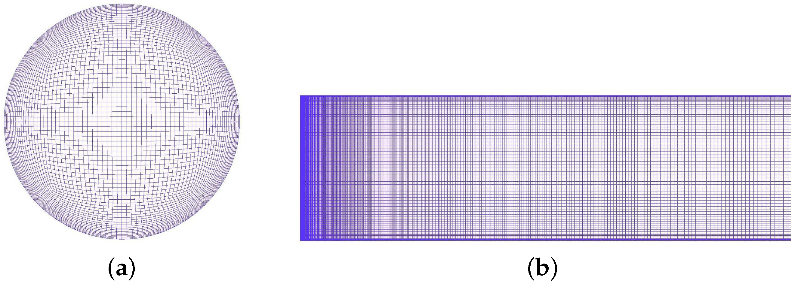
2.3.4. Boundary Conditions and Grid Resolution

The governing equations for the two models are solved with the following boundary conditions:

• At the inlet ($z=0$):

  $$w=w_{in},u=v=0,T=T_{in}=293K$$

  (27)
• On the pipe wall ($r=R=D/2$):

  $$u=v=w=0,-k_{eff}\frac{\partial T}{\partial r}{|}_{r=R}=q_w$$

  (28)
• At the pipe outlet, the gauge pressure is set equal to zero and all the normal diffusion fluxes and the mass balance correction are applied.

Several different grid distributions were tested to ensure the independence of the numerical results to the grid size. A structured mesh is used throughout the domain, with 140 nodes in the circumferential direction, 220 in the radial direction and 800 in the axial direction. A grid refinement close to the wall and in the pipe entrance is deemed necessary, where the highest velocity and temperature gradients occur (see Figure 2). This mesh grid provides grid-independent solutions for all cases studied.

The calculations are performed in parallel using Mammouth Parallel 2 of the Calcul Québec cluster with 2 nodes having each 8 processors. The convergence is typically reached after 4000 iterations corresponding to a CPU time of about 6 h.

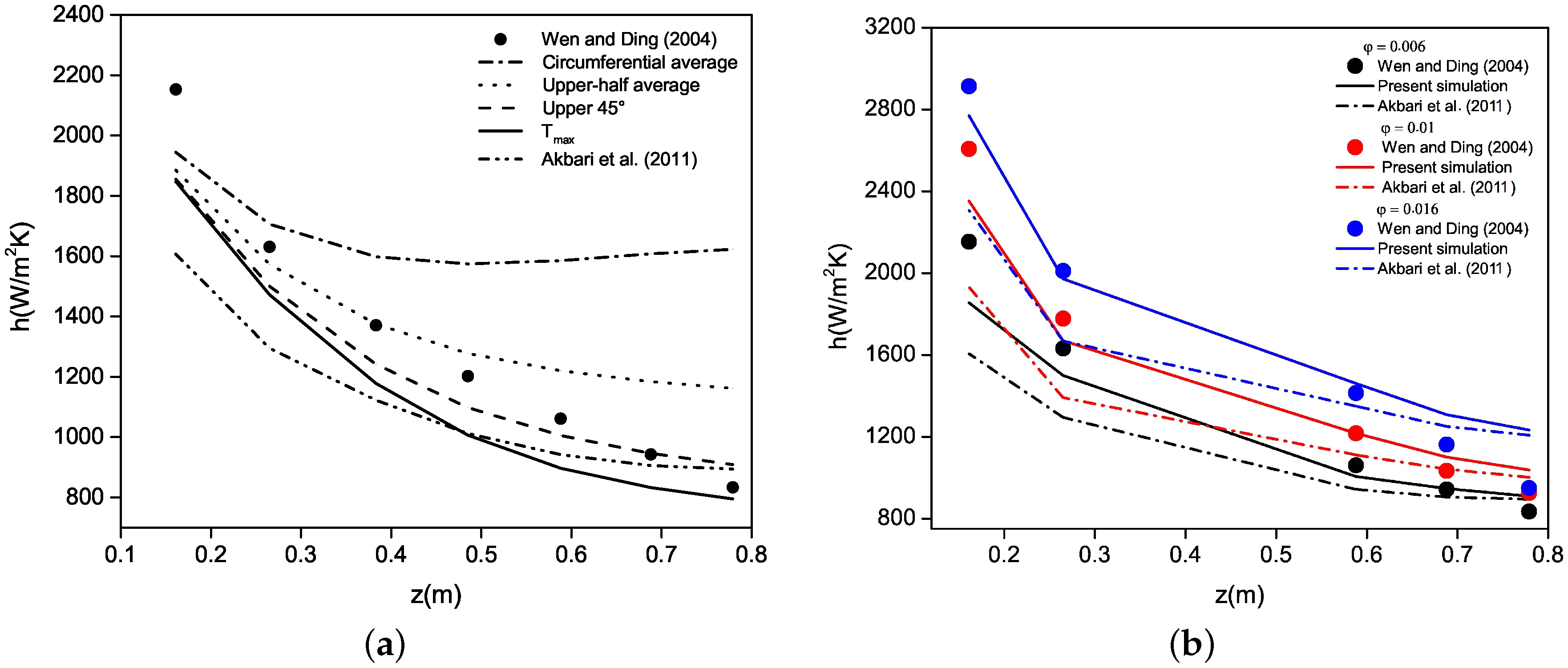
3. Validation of the Numerical Model

In this section, the results are discussed in terms of the inlet Reynolds number $Re=w_{in}D/{\nu }_{nf}$. The maximum value of the Richardson number reached here is $R{i}_{max}=Gr/R{e}^2=0.0115$, which ensures that a forced convection regime is achieved ($Gr$ the Grashof number based on D, the nanofluid properties and the temperature difference $T_{r=R,max}-T_{in}$) for all the cases studied.

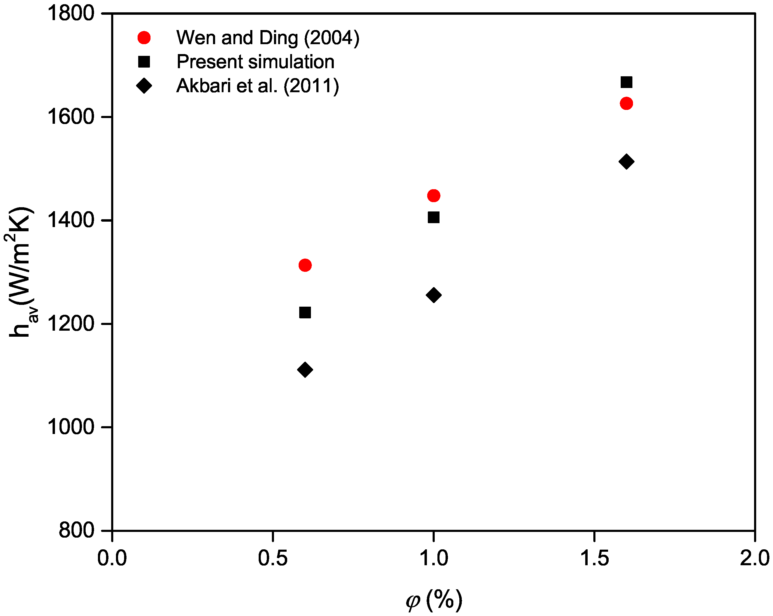
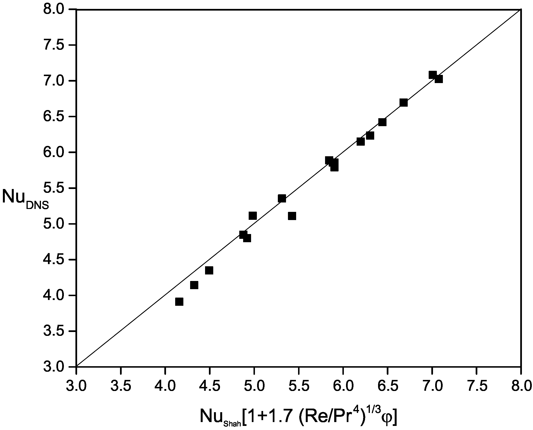
3.1. Performances of the Mixture Model

In order to first validate the selected numerical model, the local heat transfer coefficient $h(z)$ is evaluated along the pipe length. The mixture model is used together with temperature-dependent properties for water and Equations (7) and (10) for the nanoparticle properties. Due to the lack of precise information on the temperature measurement procedure in the experiments of Wen and Ding [11], four different averaging methods are used to evaluate the wall temperature of the simulated cases. Comparisons with the measurements of Wen and Ding [11] and the numerical simulations of Akbari et al. [19], for $Re=1600$ and $\mathsf{\phi }=0.6$%, are performed using the mixture model. Figure 3a illustrates that using an average over an upper arc of ±45${}^{\circ }$ leads to closer results to the experiments with an average error between $0.37\%$ and $13.84\%$ along the pipe. The temperature was probably measured experimentally near the top of the tube where the fluid is warmer due to buoyancy forces. This averaging method will be used adopted for the remainder of the study.

Figure 3b compares the values of the convective heat transfer coefficient $h(z)$ of the present simulations with the numerical results of Akbari et al. [19] and the experimental data of Wen and Ding [11] for $Re=1600$ and three volume fractions of $A{l}_2{O}_3$ nanoparticles $\mathsf{\phi }=0.6\%$, $1\%$ and $1.6\%$, respectively. The present numerical results agree fairly well with the experiments [11] with an exponential decrease of the heat transfer coefficient along the tube as expected from energy balance equation. The main discrepancy is observed close to the inlet due to the choice of the boundary conditions in the present calculations. It is noteworthy that the present simulations improve the predictions of Akbari et al. [19] using exactly the same solver and methods. It points out in particular the necessity to use an appropriate mesh grid in the near-wall regions and globally a more dense grid. Compared to [19], the number of mesh points is multiplied by a factor 86. The mesh grid sensitivity studies are generally performed using small increments of values such that no noticeable effect is observed.

Figure 4 provides further comparisons in terms of the average heat transfer coefficient $h_{av}$ for the same three cases. The present results obtained using the mixture model show an acceptable agreement with the experimental ones. The numerical data exhibit an average enhancement of about $36\%$ with increasing $\mathsf{\phi }$ from $0.6\%$ to $1.6\%$, which is to be compared to the value $24.3\%$ in the experiments. Once again, the present simulations improve the previous ones of Akbari et al. [19] pointing out the influence of the mesh grid. This improvement may be attributed to the increase of the thermal conductivity and some authors [11,12,40] proposed that it is also associated to the decrease of the thermal boundary layer thickness.

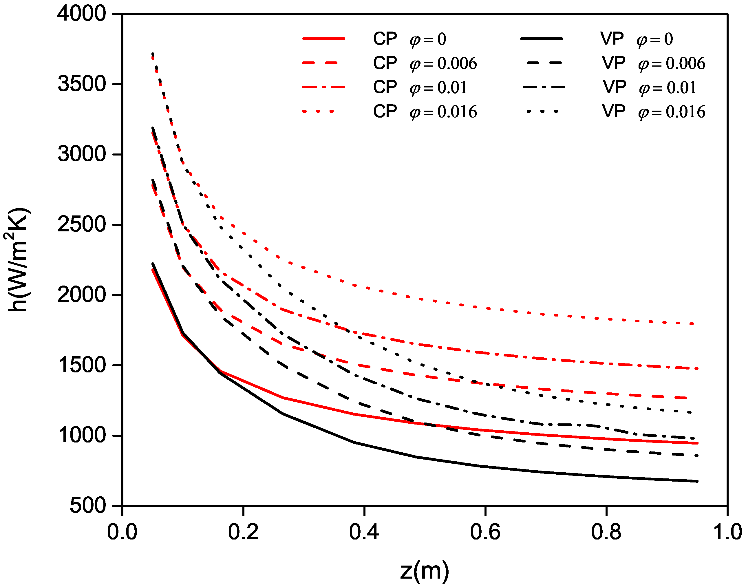
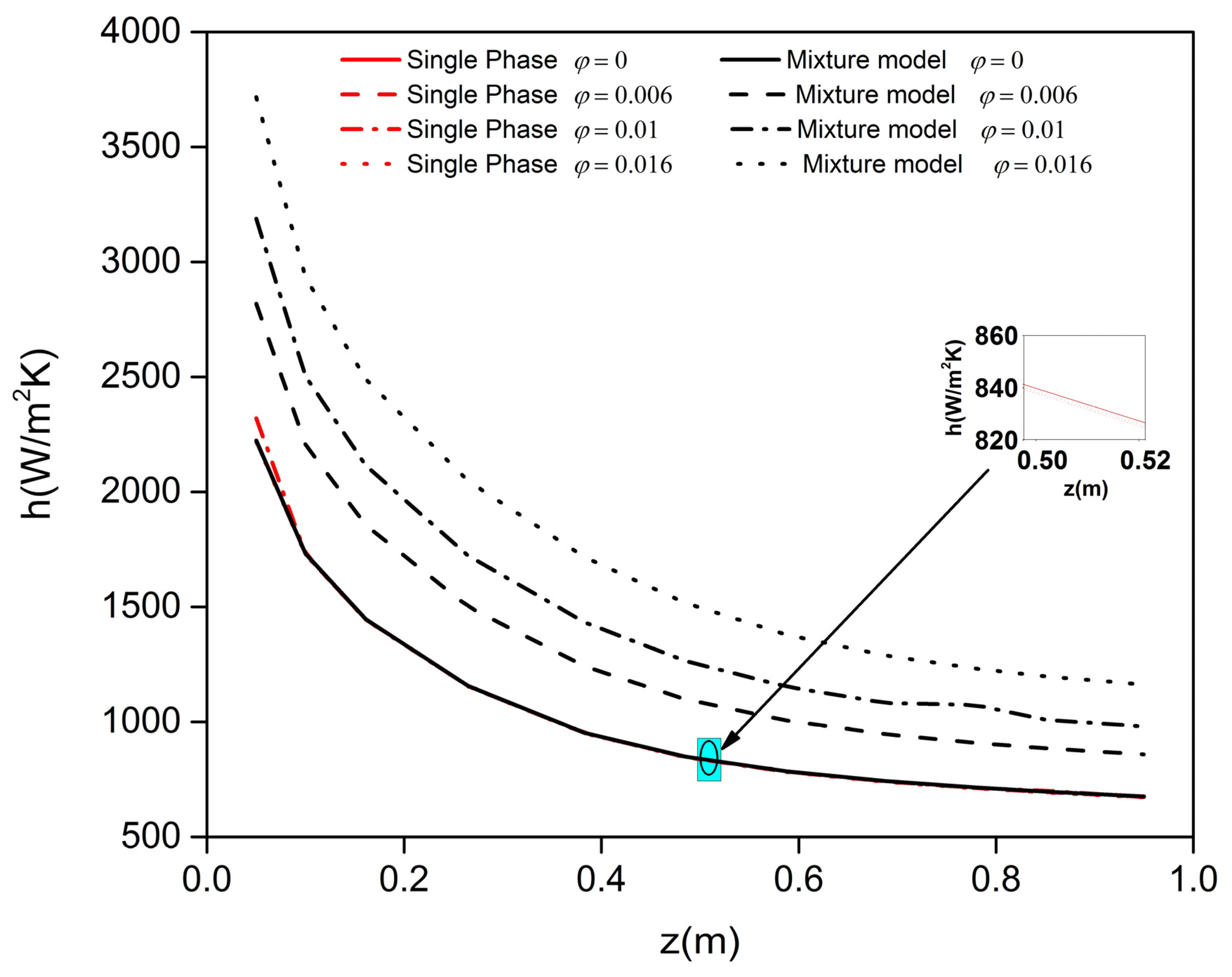
3.2. Comparative Analysis of Single-Phase and Mixture Models

Many authors [18,19,30,41] have already shown that the mixture model performs better than single-phase or other two-phase models like the Eulerian or volume of fluid models. Nevertheless, it is crucial to use appropriate correlations for the effective nanofluid properties to obtain accurate results with single-phase models.

First, the single-phase (using Equations (7) and (10) for ${\mathsf{\mu }}_{nf}$ and $k_{nf}$ respectively) and the mixture models with temperature-dependent are compared in Figure 5 for $Re=1600$ and four concentrations of nanoparticles. The single-phase model fails to predict the right axial distributions of the local heat transfer coefficient $h(z)$. An exponential decrease of $h(z)$ with the axial distance z is observed however with a noticeable underestimation for all cases with $\mathsf{\phi }\ne 0$. As expected, for $\mathsf{\phi }=0$, both models predict the same profile. Though the nanofluid properties take into account the volume fraction of nanoparticles $\mathsf{\phi }$, the single-phase model appears insensitive to $\mathsf{\phi }$ as the same heat transfer coefficient distribution is obtained whatever the value of $\mathsf{\phi }\le 0.016$. This confirms the previous results of Akbari et al. [19] and Bianco et al. [17]. On the other hand, the heat transfer coefficient predicted by the mixture model clearly increases with increased nanoparticle concentration in agreement with previous observations [18,19,30,41].

The superiority of the mixture model may be easily explained. In fact, the latter ensures a more accurate treatment of the two-phase mixture, compared to the single-phase model, which does not take into account either the spatial variations of the distribution in nanoparticles in the base fluid, nor the relative velocity of each phase. The mixture model seems a better model to describe the nanofluid flow. In fact, the slip velocity between the fluid and the nanoparticles is not zero due to several factors such as the Brownian motion or gravity, which induces for example the sedimentation of the solid particles.

One could argue that the single-phase model does not perform well due to inappropriate correlations for the thermal conductivity and the dynamic viscosity of the nanofluid. Thus, several correlations have been tested and the results are summarized in

Table 2. Influence of the different correlations on the average heat transfer coefficient $h_{av}$ (W·m${}^{-2}·$K${}^{-1}$) for $Re=1600$, $d_{np}=42$ nm and $A{l}_2{O}_3$-water based nanofluids. The relative error is given in brackets. Simulation 1 combines Equations (7) and (10), whereas simulation 2 uses Equations (8) and (9). Results obtained using the single-phase model.

$\mathsf{\phi }$	Experiments [11]	Simulation 1	Simulation 2
$0.006$	$1313.54$	$1089.66$	$1086.37$
		($17.04\%$)	($17.29\%$)
$0.016$	$1626.12$	$1085.69$	$1075.72$
		($33.23\%$)	($33.85\%$)

for $Re=1600$, $d_{np}=42$ nm and $A{l}_2{O}_3$-water based nanofluids. Two volume fractions $\mathsf{\phi }=0.006$ and $0.016$ have been considered. Simulation 1 combines Equations (7) and (10), whereas simulation 2 uses Equations (8) and (9). It is clear that the two sets of correlations provide rather the same results in terms of the average value of the heat transfer coefficient with differences of about $17\%$ and $33\%$ for $\mathsf{\phi }=0.006$ and $0.016$, respectively, compared to the experiments. It shows in particular that for these sets of parameters, the correlations do not considerably influence the accuracy of the single-phase model. As shown previously, the results are not influenced by the particle volume fraction. Though the effect of Brownian motion is accounted for in Equation (10), it has no noticeable influence in laminar flows. This confirms the previous work of Keblinski et al. [42], who suggested that the motion of nanoparticles due to the Brownian motion is too slow to transport a significant amount of heat through a nanofluid. They ignored the effect of Brownian motion in the enhancement of thermal conductivity of nanofluids.

For the sake of simplicity when developing new numerical models, it may be interesting to consider the mixture model with constant properties if satisfactory results may be obtained. Figure 6 displays the axial distributions of the local heat transfer coefficient for $Re=1600$, $d_{np}=42$ nm and $A{l}_2{O}_3$-water based nanofluids with four concentrations of nanoparticles. The results are obtained using Equations (7) and (10) either with constant (CP) or variable (VP) properties for the base fluid. In all cases, the local heat transfer coefficient h decreases exponentially with the axial distance z. Using temperature-dependent properties (VP) leads to very satisfactory results as already shown in Figure 3a. On the contrary, using constant properties (CP) leads to a strong overestimation of the heat transfer coefficient, with more pronounced differences towards the thermally fully developed flow region. In fact, the thermal conductivity of the nanofluid increases drastically with decreasing values of both temperature and density. Using VP, the circumferential wall temperature appears to be non-uniformly distributed in the tangential direction, whereas the CP model exhibits a more uniform and axisymmetric behavior. The VP model takes then into account buoyancy effects, which result in a noticeable increase of the fluid temperature in the upper half of the pipe. This confirms previous results such as those suggested by [17] except from the previous work of Labonte et al. [16], who showed that CP lead to an underestimation of the heat transfer coefficient. This difference may be attributed to the different multiphase models used.

It is important to note that taking into account temperature-dependent properties does not increase the computational cost. Using the same mesh grid, both calculations take about 4 h using 8 processors on Mammouth Parallel 2. Calculations using VP lead to a rather faster convergence as compared to the CP case.

4. Results and Discussion

All the results presented in the following have been obtained using the mixture model with temperature-dependent properties and Equations (7) and (10) to model the nanofluid properties. The influence of the Reynolds number $Re$, the volume fraction $\mathsf{\phi }$, the diameter $d_{np}$ of the nanoparticles and the type of nanoparticles on the hydrodynamic and the thermal fields are successively discussed in details in the following sections.

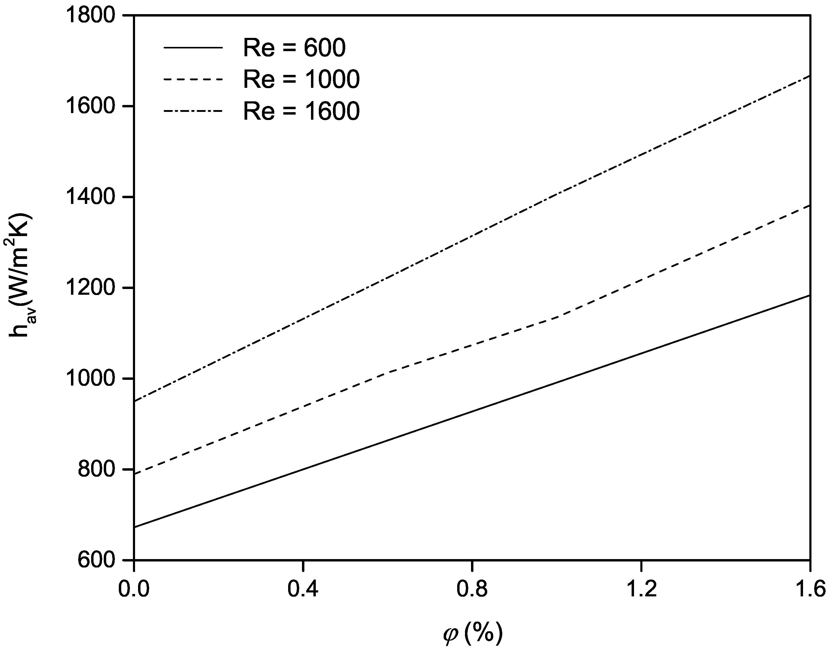
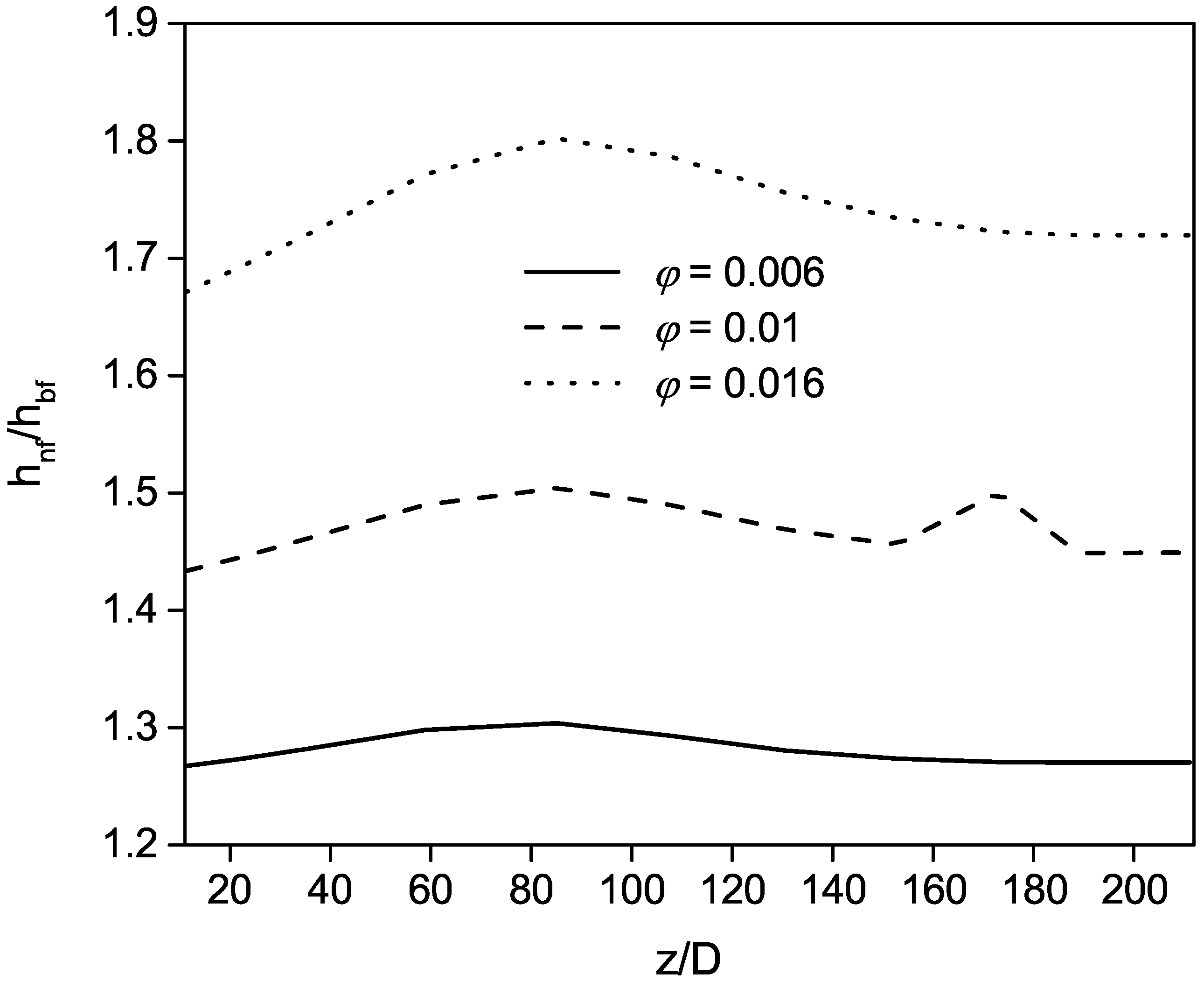
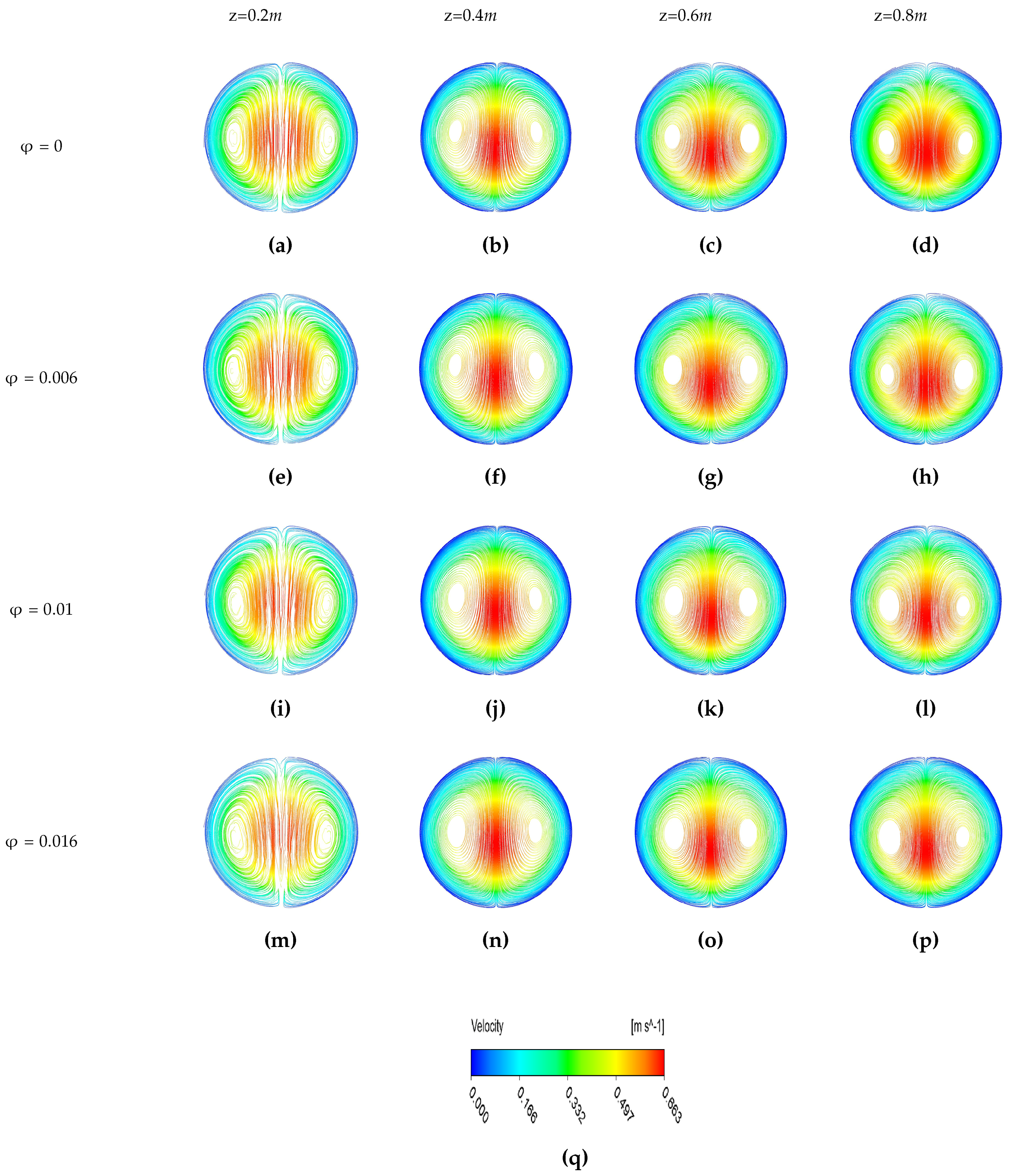
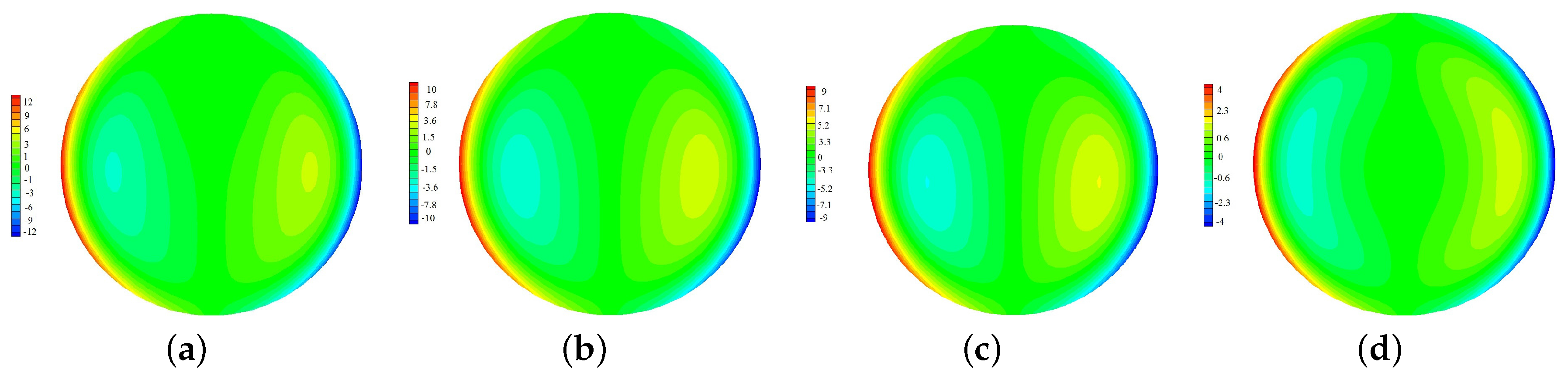
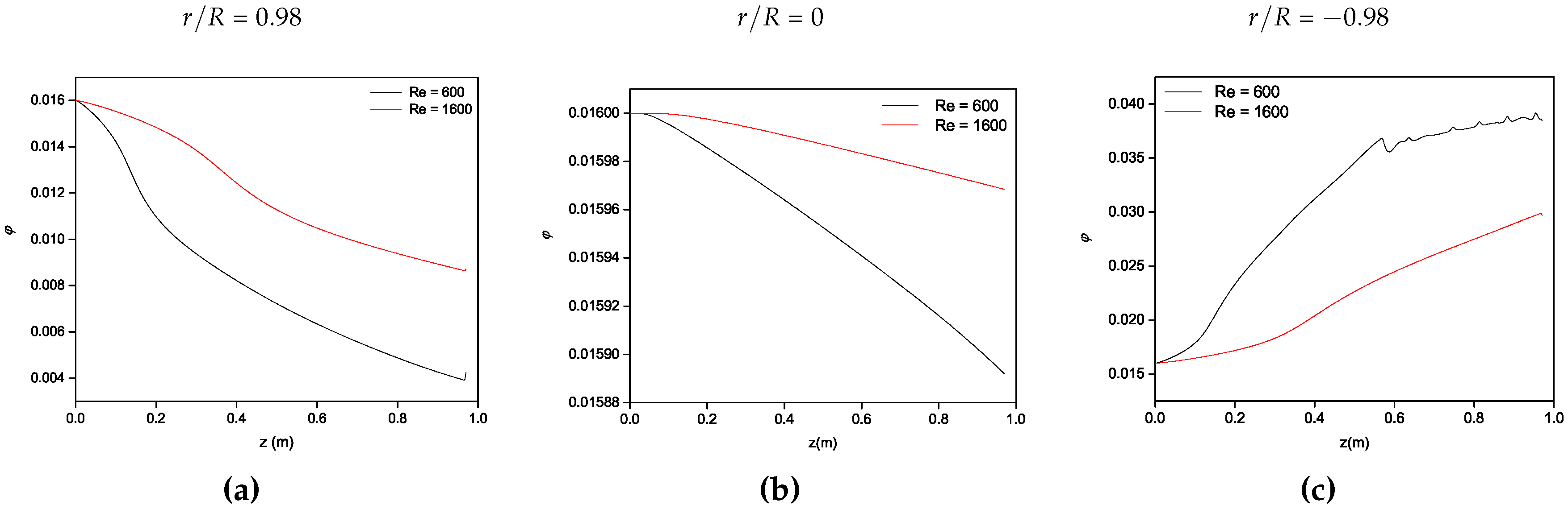
4.1. Influence of the Volume Fraction of Nanoparticles and Reynolds Number for $A{l}_2{O}_3$/Water-Based Nanofluids

The combined effects of the Reynolds number and the volume fraction of nanoparticles on the average heat transfer coefficient are plotted in Figure 7. It can be clearly observed that an average enhancement of the convective average heat transfer coefficient of about $40\%$ is achieved when the Reynolds number increases from $Re=600$ to 1600 for all nanoparticle concentrations $\mathsf{\phi }$. A linear dependency of $h_{av}$ is obtained against to $\mathsf{\phi }$ for the three $Re$ numbers.

Figure 8 shows the axial distribution of the heat transfer coefficient ratio $h_{nf}/h_{bf}$ along the pipe for $d_{np}=42$ nm, $Re=1600$ and three volume fractions of $A{l}_2{O}_3$ nanoparticles. It clearly indicates an average thermal enhancement of $28\%$, $48\%$ and $75.6\%$ for $\mathsf{\phi }=0.006$, $0.01$ and $0.016$, respectively. This ratio $h_{nf}/h_{bf}$ is rather constant in the axial direction $z/D$ with a local maximum around $z/D\simeq 85$ whatever $\mathsf{\phi }$ and a second local maximum at $z/D\simeq 175$ for $\mathsf{\phi }=0.01$.

Figure 9 illustrates the temperature contours at four axial positions $z=0.2$ m ($z/D=44.4$), $0.4$ m ($z/D=88.9$), $0.6$ m ($z/D=133.3$) and $0.8$ m ($z/D=177.8$) for $d_{np}=42$ nm, $Re=1600$ and four concentrations $\mathsf{\phi }$. The temperature contours change from a circular form at $z=0.2$ m, to an elliptical one at $z=0.4$ m then to a kidney shape from $z=0.6$ m to the tube outlet for all concentrations of nanoparticles. The circumferential wall temperature appears to be non-uniformly distributed in the tangential direction, especially at $z=0.8$ m, with maximum values at the top of the tube. It can be simply explained by density variations, since the warm nanofluid has a lowest density and can rise due to the buoyancy force to the upper half of the tube inducing a stratification of the fluid temperature. This suggests the necessity to consider temperature-dependent properties for the nanofluid in order to predict this effect. The hot temperature region located at the top of tube for $\mathsf{\phi }=0$ shown in Figure 9d progressively disappears when increasing the nanoparticle volume fraction. For example, the wall temperature $T_w$ decreases noticeably when $\mathsf{\phi }$ increases: at $z=0.8$ m, the maximum wall temperature decreases from 332 K to 293 K for $\mathsf{\phi }=0$ (Figure 9d) and $\mathsf{\phi }=0.016$ (Figure 9p), respectively. The maximum temperature difference is inversely proportional to the nanoparticle volume fraction. It is reduced almost by a factor 2 between $\mathsf{\phi }=0.016$ and $\mathsf{\phi }=0$. More generally, the introduction of even higher volume fractions (for this range of parameters) tends to homogeneize the temperature distribution at a given cross-section. It may be explained by considering nano-convection effect, which is linearly related to $\mathsf{\phi }$ [43]. This effect is induced by the Brownian motion of the nanoparticles. Brownian motion caused by the thermal interaction between the nanoparticles and the base fluid is stronger within regions of higher fluid temperature that is why the upper half of the tube is more affected. The influence of Brownian force on the thermal conductivity enhancement is strongly debated in the scientific community, some authors assume that it plays a key role [43,44], while others ignore its effect [42].

Note that the same phenomena are observed for the two other values of the Reynolds number.

Figure 10 displays the corresponding streamlines colored by the axial velocity component w at four cross-sections along the pipe. Due to the increased temperature at the wall, a secondary flow is observed. It consists of a pair of symmetrical counter-rotating vortices with respect to the tube axis. These vortices are induced by buoyancy forces: an upward flow restricted in a thin layer along the wall rises up a warm fluid and a downward flow along the tube axis drops a cool fluid [45,46]. For pure water ($\mathsf{\phi }=0$), Figure 10a shows clearly that the buoyancy force already appears at $z=0.2$ m and induces the secondary flow. The contours of the axial velocity component are axisymmetric at this axial position for all nanoparticle concentrations and the recirculation cells are symmetric. This indicates that the velocity is not yet affected by the buoyancy force, which is due to the fact that, at this location, the circumferential temperature gradients are very small.

When the fluid moves further downstream, the recirculations are slightly shifted and moves across the median plane, above the plane at $z=0.4$ m and just below the plane at $z=0.8$ m, for all values of $\mathsf{\phi }$. The maximum value of w is also slightly shifted downward below the horizontal tube axis when moving to the pipe outlet. This shift results from the important increase in the intensity of the secondary flow. This loss of axisymmetry is due to both the boundary layer development and the increasing influence of the buoyancy force, which becomes more pronounced along the tube, increasing then the strength of the secondary flow. At $z=0.8$ m, the axial velocity contours exhibit an ellipsoid-shaped form for $\mathsf{\phi }=0$. At the same time, the circular streamlines in the lower half of the tube indicate a weaker secondary flow, while the curved ones in the upper half indicate that a hot fluid is confined and accompanied by a more intense secondary flow. At $z=0.8$ m, the form of the axial velocity contours change from an ellipsoid-shaped pattern for $\mathsf{\phi }=0$ to a rather more circular form for $\mathsf{\phi }=0.016$ as illustrated in Figure 10d,p, respectively. For $\mathsf{\phi }=0.016$, the shape of the velocity contours remains practically unchanged indicating a fully developed region from z = 0.4 m. This result agrees well with the previous observations confirming that the nanoparticles suppress the buoyancy force induced secondary flow, stabilizes the flow with a strong homogeneity of the fluid temperature within the tube.

The same behavior is observed for all volume fractions of nanoparticles indicating that the latter has no remarkable influence on the hydrodynamic field. Nevertheless, the intensity of the secondary flow decreases when increasing $\mathsf{\phi }$ for all axial positions especially at $z=0.8$ m as shown in Figure 11. This is consistent with previous observations [47,48,49]. The wall layer vorticity also decreases with increased values of $\mathsf{\phi }$. The weak influence of the nanoparticle concentration on the velocity and temperature fields results from the ability of nanoparticles to homogenize the fluid temperature and therefore impeding buoyancy forces. Only few studies considered the influence of the nanoparticles on the development of the secondary flow and the homogenization of the temperature field. When $\mathsf{\phi }$ is increased, the molecular diffusion increases accompanied with an increase in the thermal conductivity and a reduction in the specific heat capacity, as proposed by [48]. Colla et al. [49] invoke the role of the Brownian diffusion.

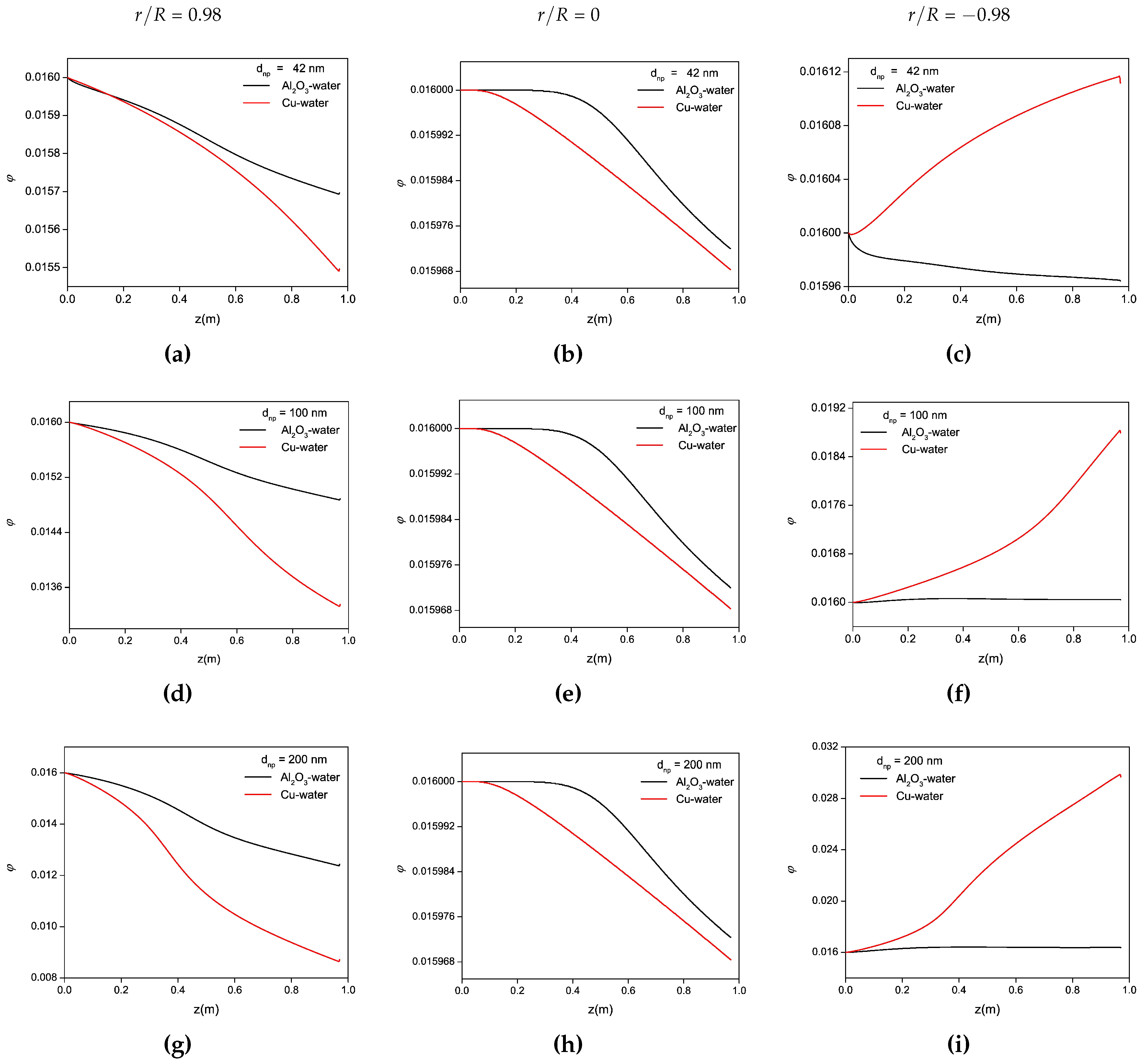
4.2. Influence of the Nanoparticle Diameter for $A{l}_2{O}_3$ and Cu/Water-Based Nanofluids

In real thermal engineering applications, increasing the nanoparticle diameter leads to higher agglomeration effects resulting in the sedimentation of the agglomerates. Such particle-particle interactions are not taken into account in the present model. Only the Brownian motion and the ratio between gravity and buoyancy forces are modeled here. The nanoparticle diameter $d_{np}$ has then no remarkable effect on the heat transfer coefficients as it will be shown in the following. More interestingly however, the influence of $d_{np}$ on the axial distributions of the nanoparticle concentration $\mathsf{\phi }$ is quite remarkable.

Figure 12 displays the axial profiles of $\mathsf{\phi }$ at three radial locations $r/R=0.98$ (top wall), $r/R=0$ (axis) and $r/R=-0.98$ (bottom wall) for two types of nanofluid (copper and alumina water-based), three nanoparticle diameters $d_{np}=42$, 100 and 200 nm and for $Re=1600$ and $\mathsf{\phi }=1.6\%$. Firstly, the concentration is rather constant along the center line of the tube ($r/R=0$) for the two nanofluids and all the nanoparticle diameters, remaining between $1.6\%$ and $1.596\%$. For $d_{np}=42$ nm, along the top wall of the tube, the nanoparticle concentration decreases by $1.5\%$ and $3\%$ for $A{l}_2{O}_3$ and Cu nanoparticles, respectively (Figure 12a). As the nanoparticle diameter grows, the concentration decreases along the top wall due to gravity effects. For example, $\mathsf{\phi }$ is reduced by $22.5\%$ and $43.75\%$ for $A{l}_2{O}_3$ and Cu nanoparticles, respectively, for $d_{np}=200$ nm. By conservation of the average value of $\mathsf{\phi }$ at a given cross-section, the concentration of nanoparticles along the bottom wall increases. Because of their higher density, this effect is more noticeable for copper/water-based nanofluids as illustrated in Figure 12c,f,i. The latter shows that $\mathsf{\phi }$ increases by $0.75\%$, $17.5\%$ and $87.5\%$ for $d_{np}=42$, 100 and 200 nm, respectively. The concentration of $A{l}_2{O}_3$ appears quite constant, with an increase of only $2.5\%$ for $d_{np}=200$ nm. This behavior can be easily explained since the density of copper is twice the alumina one.

The influence of the mean diameter of the $A{l}_2{O}_3$ nanoparticles on the heat transfer is not shown here, but it can be noticed that increasing $d_{np}$ does not affect the average heat transfer coefficient. For $\mathsf{\phi }=0.016$ and $Re=1600$, $h_{av}=1796.7$ W/m${}^2$ K and $1795.5$ W/m${}^2$ K for $d_{np}=10$ and 200 nm, respectively. However, the average heat transfer coefficient may be strongly modified by the size of the nanoparticles for copper-water nanofluids, which sediment more with only $12\%$ of the particles still in suspension in the base fluid as shown previously for $d_{np}=200$ nm (Figure 12g,i).

Figure 13 illustrates the effect of the global Reynolds number $Re$ on the distributions of the concentration in copper nanoparticles along the tube for $d_{np}=200$ nm, $\mathsf{\phi }=0.016$ and two Reynolds numbers $Re=600$ and 1600 at three radial locations $r/R=0.98$ (near the top wall), $r/R=0$ (pipe axis) and $r/R=-0.98$ (near the bottom wall). Even for this large nanoparticles, the concentration of nanoparticles along the tube axis remains almost constant. Throughout the pipe length, the variation of $\mathsf{\phi }$ is $0.13\%$ for $Re=1600$ and $0.75\%$ for $Re=1600$. At $r/R=0.98$, $\mathsf{\phi }$ decreases by a factor 2 then 4 for $Re=1600$ and $Re=600$, respectively. It results in a huge increase in nanoparticle concentration at the bottom of the pipe (Figure 13c): $\mathsf{\phi }$ increases by $87.5\%$ and $137.5\%$ for $Re=1600$ and 600, respectively. Almost all the copper nanoparticles are sedimented and there are only few copper nanoparticles suspended in pure water at the top of the tube for $Re=600$. The Reynolds number plays an important role to keep the nanoparticles well dispersed in the base fluid and reduce the sedimentation process, inducing a better stability of the nanofluid and higher resulting heat transfer.

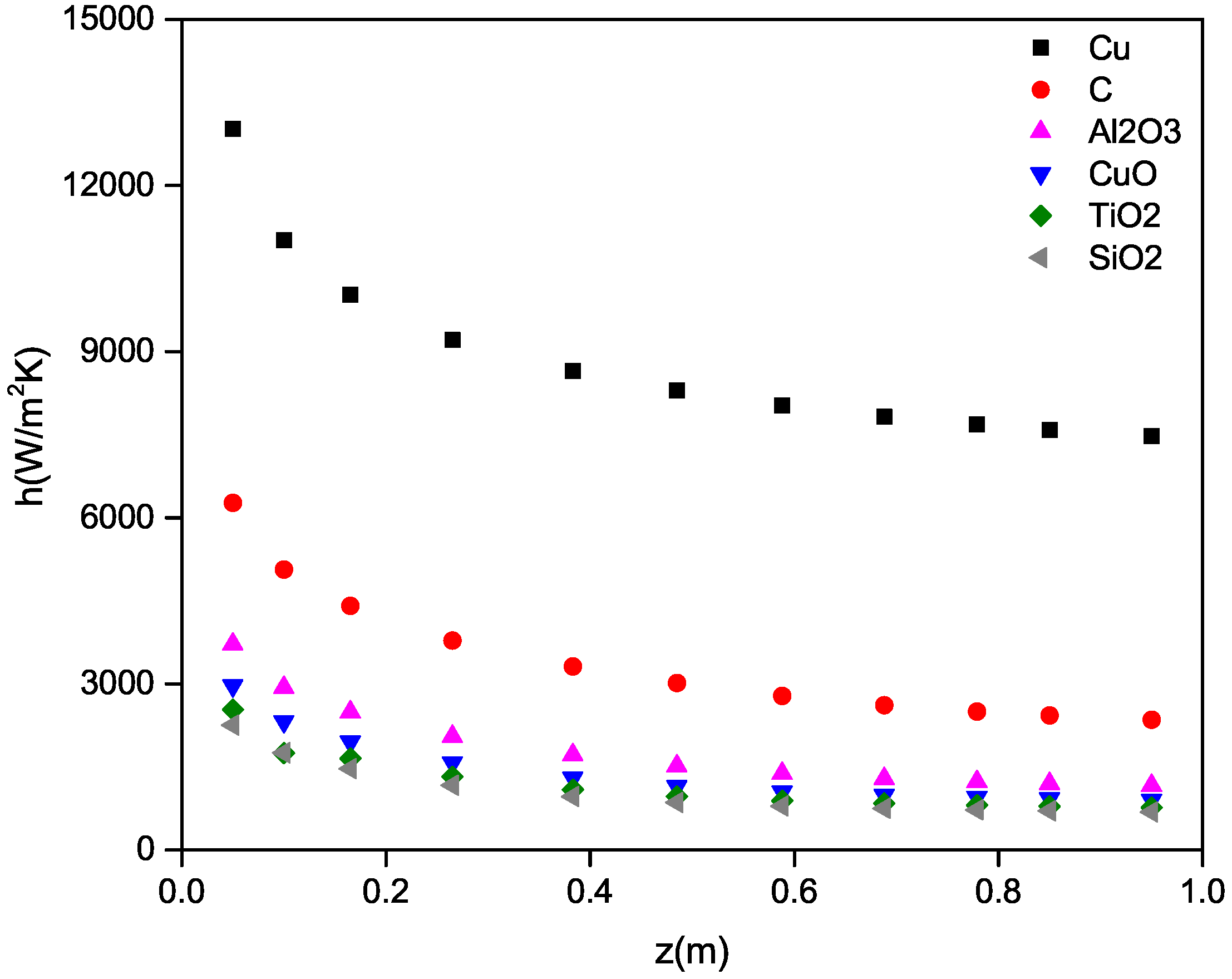
4.3. Influence of the Type of Nanoparticles for Water-Based Nanofluids

The axial variations of the heat transfer coefficient of six types of nanoparticles for $\mathsf{\phi }=1.6\%$, $d_{np}=42$ nm and $Re=1600$ are shown in Figure 14. This later figure illustrates that the local heat transfer coefficients for all water-based nanofluids exhibit the same behavior, with an exponential decrease with increased distance along the pipe. The nanofluid with copper nanoparticles achieves the highest heat transfer coefficient, followed by C, $A{l}_2{O}_3$, $CuO$, $Ti{O}_2$, and $Si{O}_2$, respectively. This behavior was expected since the copper has the highest thermal conductivity amongst the other nanofluids as shown in Table 1.

In the other hand, a major hindrance associated with the use of copper nanoparticles is the sedimentation phenomenon, as illustrated earlier for $\mathsf{\phi }=1.6\%$ and $d_{np}$ = 200 nm. They sediment 34 times higher than the $A{l}_2{O}_3$ nanoparticles under the same operating conditions. For this reason, the choice of the appropriate nanofluid does not depend only on its thermal conductivity, but should also take into account their stability and the suspension of the nanoparticles in the base fluid for a long term use.

4.4. Summary

For engineering applications, empirical correlations are of primary importance to predict the average heat transfer coefficient as a function of the flow and geometrical parameters for an effective design of thermal systems such as heat exchangers. This is particularly challenging for convective nanofluid flows as opposed to single-phase flows, because of the influence of various parameters due to the presence of the solid nanoparticles. An attempt has been done in the following. First, the well-known correlation proposed by Shah [50] for laminar flows under a constant heat flux boundary condition and used by Wen And Ding [11] is considered:

$$\begin{array}{c}\hfill N{u}_{Shah}=1.953{\left(RePr\frac{D}{x}\right)}^{1/3}33.3\le RePr\frac{D}{x}\end{array}$$

(29)

A second correlation was proposed by [50] for $RePr\frac{D}{x}\le 33.3$ but it was carefully checked here that it led to very similar results. For simplicity, only Equation (29) will be used in the following.

All the results obtained in this paper using direct numerical simulations may be expressed in terms of Nusselt number using the following correlation:

$$\begin{array}{c}\hfill N{u}_{DNS}=N{u}_{Shah}\left(1+1.7{\left(\frac{Re}{P{r}^4}\right)}^{1/3}\mathsf{\phi }\right)6.6\le RePr\frac{D}{x}\le 46.5Pr\ge 1\end{array}$$

(30)

It is noteworthy that the validity range of Equation (30) has been extended to $6.6\le RePr\frac{D}{x}\le 46.5$ compared to Equation (29). The present correlation is valid for all values tested in the present work except for the simulations involving copper nanoparticles for which $Pr\le 1$. Both geometrical (through x and D) and flow ($Re$ and $Pr$) parameters are considered in Equation (30). The influence of the solid nanoparticles is taken into account through $\mathsf{\phi }$ but also through their thermophysical properties used to define $Re$ and $Pr$. Figure 15 confirms that Equation (30) fits particularly well with all simulations for $Pr\ge 1$.

The second term $1.7{\left(Re/P{r}^4\right)}^{1/3}\mathsf{\phi }$ in Equation (30) is small compared to 1 in all cases. The results are then well fitted with Equation (29) and so with the correlation provided by Rea et al. [35] for $A{l}_2{O}_3$/water-based nanofluids, $431\le Re\le 2000$ and $\mathsf{\phi }\le 0.06$. It corresponds to Equation (29) with a prefactor equal to $2.0398$ instead of $1.953$.

The second interesting quantity for engineering applications is the variations of the average friction factor $f_{av}$ as a function of the Reynolds number $Re$. The friction factor is calculated as proposed by Choi and Cho [51]:

$$f=\frac{8{\tau }_w}{\mathsf{\rho }{u}_m^2}$$

(31)

where $u_m$ is the mean fluid velocity and ${\tau }_w$ is the wall shear stress. It may be convenient to find correlations under the form: $f=AR{e}^{\mathsf{\alpha }}$. Figure 16 summarizes the results obtained for $A{l}_2{O}_3$/water-based nanofluids with alumina nanoparticles of diameter $d_{np}=42$ nm and for four volume fractions $\mathsf{\phi }$. As for pure water flows, the average friction factor $f_{av}$ decreases for increased values of $Re$. Complementary calculations have been performed for turbulent flows up to $Re=15,000$. In the laminar regime, $f_{av}$ varies according to the relation $f_{av}=11.381R{e}^{-0.756}$, whereas, in the turbulent regime, $f_{av}$ follows: $f_{av}=1.05R{e}^{-0.358}$. A discontinuity is also observed in the transitional regime. The presence of nanoparticles in the base fluid affects the variations of the average friction factor compared to pure water flows. However, the friction factor $f_{av}$ appears to be insensitive to the nanoparticle concentration $\mathsf{\phi }$. The results are to be compared to the classical Darcy relations for single-phase flows in pipes, where: $A=64$ and $\mathsf{\alpha }=-1$ for laminar flows and $A=0.3164$ and $\mathsf{\alpha }=-0.25$ for turbulent flows in smooth pipes.

In the laminar regime, the results agree particularly well with the correlation of Suresh et al. [52] obtained for $A{l}_2{O}_3$-Cu/water-based nanofluid with $Re<2300$ and $\mathsf{\phi }\le 0.1\%$: $A=26.4f(\mathsf{\phi })$ and $\mathsf{\alpha }=-0.8737$.

5. Conclusions

Laminar forced convection flows of water-based nanofluids through a uniformly heated tube were revisited here using direct numerical simulations. The single-phase and mixture models with constant and temperature-dependent properties were compared to the experimental data of Wen and Ding [11] and to the numerical simulations of Akbari et al. [19]. The mixture model with temperature-dependent properties was shown to perform best with a close agreement to the experimental data. The former simulations of Akbari et al. [19] using the same model were significantly improved with the use of an appropriate mesh grid.

The numerical model was then used confidently and extensively to investigate the influences of the Reynolds number ($600\le Re\le 1600$), the concentration in nanoparticles ($\mathsf{\varphi }\le 1.6\%$) and their diameter ($42\le d_{np}\le 200$ nm) on the hydrodynamic and thermal fields. $A{l}_2{O}_3$/water based nanofluids have been considered first before evaluating the thermal performances of other nanoparticles such as: $Cu$, C, $CuO$, $Ti{O}_2$, and $Si{O}_2$.

For $A{l}_2{O}_3$/water based nanofluids, the average heat transfer coefficient increased linearly with the nanoparticle concentration for all Reynolds numbers. At $Re=1600$, the local heat transfer coefficient increased in average by $29\%$, $46\%$ and $74\%$ for $\mathsf{\phi }=0.006$, $0.01$ and $0.016$, respectively. Increasing the nanoparticle concentration led to a more homogenous temperature field, impeding the hot temperature region observed at the top of the pipe wall for pure water flows. The flow field revealed two recirculation regions for all ($r,\mathsf{\theta }$) planes, only weakly influenced by $\mathsf{\phi }$. The maximum value of the axial velocity component observed at ($r/R\simeq -0.2$, $\mathsf{\theta }=-{90}^{\circ }$) was also weakly affected by $\mathsf{\phi }$. The volume fraction in nanoparticles affected significantly the streamwise vorticity of the two recirculation cells. The flow and temperature fields exhibited a more homogeneous behavior. A particular attention was also paid to the sedimentation of the nanoparticles, which, as expected, increased for large size or high density nanoparticles. Finally, empirical correlations to predict both the Nusselt number and the average friction coefficient have been provided, summarizing all simulations presented here (in the range of $Pr\ge 1$ for $Nu$).

Further calculations are now required to extend the present simulations to the turbulent flow regime using large-eddy simulations. Further developments are also planned to improve the numerical model to take into account more complex phenomena like the thermophoresis effect and particle-particle interactions.

References

1. Wong, K.V.; De Leon, O. Applications of nanofluids: Current and future. Adv. Mech. Eng. 2010, 2010. [Google Scholar] [CrossRef]
2. Huminic, G.; Huminic, A. Application of nanofluids in heat exchangers: A review. Renew. Sustain. Energy Rev. 2012, 16, 5625–5638. [Google Scholar] [CrossRef]
3. Maxwell, J.C. A Treatise on Electricity and Magnetism, 2nd ed.; Clarendon: Oxford, UK, 1881. [Google Scholar]
4. Choi, S.U.S.; Eastman, J.A. Enhancing Thermal Conductivity of Fluids with Nanoparticles. In Proceedings of the ASME International Mechanical Engineering Congress & Exposition, San Francisco, CA, USA, 12–17 November 1995; Volume 231, pp. 99–106.
5. Jang, S.P.; Choi, S.U.S. Effects of various parameters on nanofluid thermal conductivity. J. Heat Transf. 2007, 129, 617–623. [Google Scholar] [CrossRef]
6. Khanafer, K.; Vafai, K. A critical synthesis of thermophysical characteristics of nanofluids. Int. J. Heat Mass Transf. 2011, 54, 4410–4428. [Google Scholar] [CrossRef]
7. Riazi, H.; Murphy, T.; Webber, G.B.; Atkin, R.; Mostafavi Tehrani, S.S.; Taylor, R.A. Specific heat control of nanofluids: A critical review. Int. J. Therm. Sci. 2016, 107, 25–38. [Google Scholar] [CrossRef]
8. Bianco, V.; Manca, O.; Nardini, S.; Vafai, K. Heat Transfer Enhancement with Nanofluids; CRC Press: London, UK, 2015. [Google Scholar]
9. Das, S.K.; Choi, S.U.S.; Yu, W.; Pradeep, T. Nanofluids Science and Technology; John Wiley & Sons, Inc.: Hoboken, NJ, USA, 2008. [Google Scholar]
10. Kakac, S.; Pramuanjaroenkij, A. Single-phase and two-phase treatments of convective heat transfer enhancement with nanofluids—A state-of-the-art review. Int. J. Therm. Sci. 2016, 100, 75–97. [Google Scholar] [CrossRef]
11. Wen, D.; Ding, Y. Experimental investigation into convective heat transfer of nanofluids at the entrance region under laminar flow conditions. Int. J. Heat Mass Transf. 2004, 47, 5181–5188. [Google Scholar] [CrossRef]
12. Heyhat, M.M.; Kowsary, F.; Rashidi, A.M.; Momenpour, M.H.; Amrollahi, A. Experimental investigation of laminar convective heat transfer and pressure drop of water-based Al2O3 nanofluids in fully developed flow regime. Exp. Therm. Fluid Sci. 2013, 44, 483–489. [Google Scholar] [CrossRef]
13. Halelfadl, S.; Estellé, P.; Maré, T. Heat transfer properties of aqueous carbon nanotubes nanofluids in coaxial heat exchanger under laminar regime. Exp. Therm. Fluid Sci. 2014, 55, 174–180. [Google Scholar] [CrossRef] [Green Version]
14. Maré, T.; Halelfadl, S.; Sow, O.; Estellé, P.; Duret, S.; Bazantay, F. Comparison of the thermal performances of two nanofluids at low temperature in a plate heat exchanger. Exp. Therm. Fluid Sci. 2011, 35, 1535–1543. [Google Scholar] [CrossRef] [Green Version]
15. Mehrez, Z.; El Cafsi, A.; Belghith, A.; Le Quéré, P. The entropy generation analysis in the mixed convective assisting flow of Cu-water nanofluid in an inclined open cavity. Adv. Powder Technol. 2015, 26, 1442–1451. [Google Scholar] [CrossRef]
16. Labonté, J.; Nguyen, C.T.; Roy, G. Heat Transfer Enhancement in Laminar Flow Using Al2O3-Water Nanofluid Considering Temperature-Dependent Properties. In Proceedings of the 4th WSEAS International Conference on Heat Transfer, Thermal Engineering and Environment, Elounda, Greece, 21–23 August 2006; pp. 21–23.
17. Bianco, V.; Chiacchio, F.; Manca, O.; Nardini, S. Numerical investigation of nanofluids forced convection in circular tubes. Appl. Therm. Eng. 2009, 29, 3632–3642. [Google Scholar] [CrossRef]
18. Lotfi, R.; Saboohi, Y.; Rashidi, A.M. Numerical study of forced convective heat transfer of nanofluids: Comparison of different approaches. Int. Commun. Heat Mass Transf. 2010, 37, 74–78. [Google Scholar] [CrossRef]
19. Akbari, M.; Galanis, N.; Behzadmehr, A. Comparative analysis of single and two-phase models for CFD studies of nanofluid heat transfer. Int. J. Therm. Sci. 2011, 50, 1343–1354. [Google Scholar] [CrossRef]
20. Azari, A.; Kalbasi, M.; Rahimi, M. CFD and experimental investigation on the heat transfer characteristics of alumina nanofluids under the laminar flow regime. Braz. J. Chem. Eng. 2014, 31, 469–481. [Google Scholar] [CrossRef]
21. Behroyan, I.; Vanaki, S.M.; Ganesan, P.; Saidur, R. A comprehensive comparison of various CFD models for convective heat transfer of Al2O3 nanofluid inside a heated tube. Int. Commun. Heat Mass Transf. 2016, 70, 27–37. [Google Scholar] [CrossRef]
22. Bianco, V.; Manca, O.; Nardini, S. Second law analysis of Al2O3-water nanofluid turbulent forced convection in a circular cross section tube with constant wall temperature. Adv. Mech. Eng. 2013, 2013, 1–12. [Google Scholar] [CrossRef]
23. Anoop, K.; Sundararajan, T.; Das, S. Effect of particle size on the convective heat transfer in nanofluid in the developing region. Int. J. Heat Mass Transf. 2009, 52, 2189–2195. [Google Scholar] [CrossRef]
24. Hwang, K.S.; Jang, S.P.; Choi, S.U.S. Flow and convective heat transfer characteristics of water-based Al2O3 nanofluids in fully developed laminar flow regime. Int. J. Heat Mass Transf. 2009, 52, 193–199. [Google Scholar] [CrossRef]
25. Wang, X.; Li, X. Influence of pH on nanofluids’ viscosity and thermal conductivity. Chin. Phys. Lett. 2009, 26. [Google Scholar] [CrossRef]
26. Liu, M.; Ding, C.; Wang, J. Modeling of thermal conductivity of nanofluids considering aggregation and interfacial thermal resistance. RSC Adv. 2016, 6, 3571–3577. [Google Scholar] [CrossRef]
27. Kakac, S.; Pramuanjaroenkij, A. Review of convective heat transfer enhancement with nanofluids. Int. J. Heat Mass Transf. 2009, 52, 3187–3196. [Google Scholar] [CrossRef]
28. Vargaftik, N.B. Tables on the Thermophysical Properties of Liquids and Gases: In Normal and Dissociated States; Hemisphere Publishing Corporation: Washington, DC, USA, 1975. [Google Scholar]
29. Chon, C.H.; Kihm, K.D.; Lee, S.P.; Choi, S.U.S. Empirical correlation finding the role of temperature and particle size for nanofluid (Al2O3) thermal conductivity enhancement. Appl. Phys. Lett. 2005, 87. [Google Scholar] [CrossRef]
30. Behzadmehr, A.; Saffar-Avval, M.; Galanis, N. Prediction of turbulent forced convection of a nanofluid in a tube with uniform heat flux using a two phase approach. Int. J. Heat Fluid Flow 2007, 28, 211–219. [Google Scholar] [CrossRef]
31. De Castro, C.A.N.; Li, S.F.Y.; Nagashima, A.; Trengove, R.D.; Wakeham, W.A. Standard reference data for the thermal conductivity of liquids. J. Phys. Chem. Ref. Data 1986, 15, 1073–1086. [Google Scholar] [CrossRef]
32. Xuan, Y.; Roetzel, W. Conceptions for heat transfer correlation of nanofluids. Int. J. Heat Mass Transf. 2000, 43, 3701–3707. [Google Scholar] [CrossRef]
33. Khanafer, K.; Vafai, K.; Lightstone, M. Buoyancy-driven heat transfer enhancement in a two-dimensional enclosure utilizing nanofluids. Int. J. Heat Mass Transf. 2003, 46, 3639–3653. [Google Scholar] [CrossRef]
34. Maiga, S.E.B.; Nguyen, C.T.; Galanis, N.; Roy, G. Heat transfer behaviours of nanofluids in a uniformly heated tube. Superlattices Microstruct. 2004, 35, 543–557. [Google Scholar] [CrossRef]
35. Rea, U.; McKrell, T.; Hu, L.; Buongiorno, J. Laminar convective heat transfer and viscous pressure loss of alumina-water and zirconia-water nanofluids. Int. J. Heat Mass Transf. 2009, 52, 2042–2048. [Google Scholar] [CrossRef]
36. Hachey, M.; Nguyen, C.; Galanis, N.; Popa, C. Experimental investigation of Al2O3 nanofluids thermal properties and rheology e effects of transient and steady-state heat exposure. Int. J. Therm. Sci. 2014, 76, 155–167. [Google Scholar] [CrossRef]
37. Nan, C.W.; Birringer, R.; Clarke, D.R.; Gleiter, H. Effective thermal conductivity of particulate composites with interfacial thermal resistance. J. Appl. Phys. 1997, 81, 6692–6699. [Google Scholar] [CrossRef]
38. Manninen, M.; Taivassalo, V.; Kallio, S. On the mixture model for multiphase flow. VTT Publ. 1996, 88, 67. [Google Scholar]
39. Schiller, L.; Naumann, Z. A drag coefficient correlation. Z. Ver. Deutsch. Ing. 1935, 77, 318–320. [Google Scholar]
40. Heris, S.Z.; Esfahany, M.N.; Etemad, S.G. Experimental investigation of convective heat transfer of Al2O3/water nanofluid in circular tube. Int. J. Heat Fluid Flow 2007, 28, 203–210. [Google Scholar] [CrossRef]
41. Bianco, V.; Manca, O.; Nardini, S. Numerical investigation on nanofluids turbulent convection heat transfer inside a circular tube. Int. J. Therm. Sci. 2011, 50, 341–349. [Google Scholar] [CrossRef]
42. Keblinski, P.; Phillpot, S.R.; Choi, S.U.S.; Eastman, J.A. Mechanisms of heat flow in suspensions of nano-sized particles (nanofluids). Int. J. Heat Mass Transf. 2002, 45, 855–863. [Google Scholar] [CrossRef]
43. Jang, S.P.; Choi, S.U.S. Role of Brownian motion in the enhanced thermal conductivity of nanofluids. Appl. Phys. Lett. 2004, 84, 4316–4318. [Google Scholar] [CrossRef]
44. Koo, J.; Kleinstreuer, C. A new thermal conductivity model for nanofluids. J. Nanopart. Res. 2004, 6, 577–588. [Google Scholar] [CrossRef]
45. Galanis, N.; Ouzzane, M. Developing mixed convection in an Inclined tube with circumferentially nonuniform heating at its outer surface. Numer. Heat Transf. A Appl. 1999, 35, 609–628. [Google Scholar] [CrossRef]
46. Orfi, J.; Galanis, N. Developing laminar mixed convection with heat and mass transfer in horizontal and vertical tubes. Int. J. Therm. Sci. 2002, 41, 319–331. [Google Scholar] [CrossRef]
47. Khdher, A.M.; Mamat, R.; Sidik, N.A.C. The Effects of Turbulent Nanofluids and Secondary Flow on the Heat Transfer through a Straight Channel. In Recent Advances in Mathematical and Computational Methods; Springer: Dordrecht, The Netherlands, 2011; pp. 118–124. [Google Scholar]
48. Ebrahimnia-Bajestan, E.; Niazmand, H. Convective heat transfer of nanofluids flows through an isothermally heated curved pipe. Iran. J. Chem. Eng. 2011, 8, 81–97. [Google Scholar]
49. Colla, L.; Fedele, L.; Buschmann, M.H. Nanofluids Suppress Secondary Flow in Laminar Pipe Flow. In Proceedings of the World Congress on Mechanical, Chemical, and Material Engineering, Barcelona, Spain, 20–21 July 2015; pp. 279-1–279-4.
50. Shah, R.K. Thermal Entry Length Solutions for the Circular Tube and Parallel Plates. In Proceedings of the Third National Heat and Mass Transfer Conference, Bombay, India, 11–13 December 1975; Volume 1, pp. 11–75.
51. Choi, M.; Cho, K. Effect of the aspect ratio of rectangular channels on the heat transfer and hydrodynamics of paraffin slurry flow. Int. J. Heat Mass Transf. 2001, 44, 55–61. [Google Scholar] [CrossRef]
52. Suresh, S.; Chandrasekar, M.; Chandra Sekhar, S. Experimental studies on heat transfer and friction factor characteristics of CuO/water nanofluid under turbulent flow in a helically dimpled tube. Exp. Therm. Fluid Sci. 2011, 35, 542–549. [Google Scholar] [CrossRef]
Figure 1. Schematic view of the computational domain with the boundary conditions.
Applsci 06 00332 g001
Figure 2. Schematic view of the mesh grid: (a) in a given cross-section; and (b) along the axial direction.
Applsci 06 00332 g002
Figure 3. Axial variations of the local heat transfer coefficient h ( z ) predicted by the mixture model for A l 2 O 3 water-based nanofluids: (a) different methods for the evaluation of the wall temperature T w for φ = 0 . 006 ; (b) three nanoparticle concentrations ( φ = 0 . 006 , 0 . 01 and 0 . 016 ). Comparisons for R e = 1600 and d n p = 42 nm with the experimental data of Wen and Ding [11] and the numerical simulations of Akbari et al. [19].
Applsci 06 00332 g003
Figure 4. Influence of the concentration of A l 2 O 3 nanoparticles φ on the average heat transfer coefficient for R e = 1600 and d n p = 42 nm. Comparisons with the experimental data of Wen and Ding [11] and the numerical simulations of Akbari et al. [19].
Applsci 06 00332 g004
Figure 5. Local heat transfer coefficient obtained for R e = 1600 , d n p = 42 nm and A l 2 O 3 -water based nanofluids: comparison between the single-phase and mixture models with temperature-dependent properties.
Applsci 06 00332 g005
Figure 6. Local heat transfer coefficient obtained for R e = 1600 , d n p = 42 nm and A l 2 O 3 -water based nanofluids: Influence of temperature-dependent properties on the performances of the mixture model.
Applsci 06 00332 g006
Figure 7. Effects of the A l 2 O 3 nanoparticle concentration φ and Reynolds number R e on the average heat transfer coefficient h a v for d n p = 42 nm.
Applsci 06 00332 g007
Figure 8. Axial variations of the heat transfer coefficient ratio h n f / h b f for d n p = 42 nm, R e = 1600 and three volume fractions in A l 2 O 3 nanoparticles: φ = 0 . 006 , 0 . 01 and 0 . 016 .
Applsci 06 00332 g008
Figure 9. Maps of temperature T at four axial positions: z = 0 . 2 m (a,e,i,m); z = 0 . 4 m (b,f,j,n); z = 0 . 6 m (c,g,k,o); and z = 0 . 8 m (d,h,l,p). Results obtained for d n p = 42 nm, R e = 1600 and four volume fractions of A l 2 O 3 nanoparticles: φ = 0 (ad); 0 . 006 (eh); 0 . 01 (il); and 0 . 016 (mp).
Applsci 06 00332 g009
Figure 10. Streamline patterns colored by the axial velocity component w at four axial positions: z = 0 . 2 m (a,e,i,m); z = 0 . 4 m (b,f,j,n); z = 0 . 6 m (c,g,k,o); and z = 0 . 8 m (d,h,l,p). Results obtained for d n p = 42 nm, R e = 1600 and four concentrations of A l 2 O 3 nanoparticles: φ = 0 (ad); 0 . 006 (eh); 0 . 01 (il); and 0 . 016 (mp).
Applsci 06 00332 g010
Figure 11. Contours of the streamwise vorticity at z = 0 . 8 m: (a) φ = 0 ; (b) φ = 0 . 006 ; (c) φ = 0 . 01 ; and (d) φ = 0 . 016 . Results obtained for d n p = 42 nm, R e = 1600 and A l 2 O 3 nanoparticles.
Applsci 06 00332 g011
Figure 12. Axial variations of the volume fraction φ at three radial locations: r / R = 0 . 98 (a,d,g); r / R = 0 (b,e,h); and r / R = 0 . 98 (c,f,i). Results obtained for C u and A l 2 O 3 nanoparticles of three different diameters d n p = 42 nm (ac); 100 nm (df); and 200 nm (gi) with φ = 0 . 016 and R e = 1600 .
Applsci 06 00332 g012
Figure 13. Axial variations of the volume fraction φ in C u nanoparticles at three radial locations: (a) r / R = 0 . 98 ; (b) r / R = 0 ; and (c) r / R = 0 . 98 . Results obtained for C u nanoparticles of diameter d n p = 200 nm with φ = 0 . 016 and two Reynolds numbers R e = 600 and 1600.
Applsci 06 00332 g013
Figure 14. Axial variations of the local heat transfer coefficient h for six types of nanoparticles with d n p = 42 nm, φ = 0 . 016 and R e = 1600 .
Applsci 06 00332 g014
Figure 15. Verification of Equation (30).
Applsci 06 00332 g015
Figure 16. Influence of the Reynolds number R e on the average friction coefficient f a v . Results obtained for all values of φ , d n p and all types of nanofluids.
Applsci 06 00332 g016