Article

Design and Implementation of an Optimal Energy Control System for Fixed-Wing Unmanned Aerial Vehicles

1
Department of Aerospace and Systems Engineering, Feng Chia University, No. 100, Wenhwa Road, Seatwen District, Taichung 407, Taiwan
2
Institute of Aeronautics and Astronautics Engineering, National Cheng-Kung University, No. 1, Daxue Road, East District, Tainan 701, Taiwan
*
Author to whom correspondence should be addressed.
Appl. Sci. 2016, 6(11), 369; https://doi.org/10.3390/app6110369
Submission received: 18 August 2016 / Revised: 29 October 2016 / Accepted: 15 November 2016 / Published: 19 November 2016

Abstract

:
In conventional flight control design, the autopilot and the autothrottle systems are usually considered separately, resulting in a complex system and inefficient integration of functions. Therefore, the concept of aircraft energy control is brought up to solve the problem of coordinated control using elevator and throttle. The goal of this study is to develop an optimal energy control system (OECS), based on the concept of optimal energy for fixed-wing unmanned aerial vehicles (UAVs). The energy of an aircraft is characterized by two parameters, which are specific energy distribution rate, driven by elevator, and total specific energy rate, driven by throttle. In this study, a system identification method was employed to obtain the energy model of a small UAV. The proposed approach consists of energy distribution loop and total energy loop. Energy distribution loop is designed based on linear-quadratic-Gaussian (LQG) regulator and is responsible for regulating specific energy distribution rate to zero. On the other hand, the total energy loop, based on simple gain scheduling method, is responsible for driving the error of total specific energy rate to zero. The implementation of OECS was successfully validated in the hard-in-the-loop (HIL) simulation of the applied UAV.

Graphical Abstract

1. Introduction

Driven by advanced computing technologies, open-source systems, investigations and applications of unmanned aerial vehicles (UAVs) have progressed at an astounding speed in the past decades. To extend the applications of UAVs in wide area or long range, the fuel efficiency of the propulsion system plays a key role in this topic. In general, a fixed-wing aircraft has higher aerodynamic efficiency than a rotorcraft, which implies that it has better endurance and range than the rotorcraft. It can provide the advantage of longer flight durations at higher speeds thus enabling larger survey areas per given flight. Both the range and endurance of an aircraft depend on rate of fuel consumption of the engine. Therefore, the flight control design plays an important role in the optimization of the fuel consumption for an aircraft or UAV. In conventional flight control design, the autopilot and the autothrottle systems are usually considered separately [1]. The autothrottle unit is mainly used to adjust the engine throttle valve to achieve the desired flight speed, and the autopilot unit is designed to regulate the control surfaces for attitude and altitude maneuvers. However, since the dynamic model of an aircraft is nonlinear and uncertain, interaction between autopilot and autothrottle systems actually exists, and dynamic coupling between speed and altitude always occurs.
According to the study proposed by Denker [2], a pilot who tries to control airspeed and altitude separately winds up controlling one or the other rather poorly. Often times, the airspeed gets too low, whereupon the wing stalls and the pilot abruptly loses control. There is a coupling effect between airspeed and altitude, and controlling either one will affect another. In conventional flight control system, airspeed is controlled by throttle and altitude is controlled by elevator. This method will cause the undesirable flight path and airspeed coupling, and loss of airspeed control when thrust is limited. Therefore, by utilizing the relationship between airspeed and altitude, a control system was introduced by utilizing the energy of an aircraft. The first energy-based flight control system, named total energy control system (TECS), was developed by Lambregts [3,4]. TECS is a generic control technique that integrates all longitudinal flight-path and speed control functions, which does not depend on a particular aircraft type [5]. For fixed-wing aircraft, the mechanism and applications of TECS were used in guidance [6,7] and flight control [5,8,9]. TECS based controllers have been successfully implemented on many aircrafts, such as the National Aeronautics and Space Administration (NASA) B737 technology demonstration plane [10], a general aviation aircraft [11], and a motor glider [12]. For helicopter, the design of a flight control system using TECS and H control theory was introduced in the study [1].
Recently, studies based on TECS for UAVs have attracted more and more attention. However, compared to manned aircrafts, there are relatively few studies focused on the fuel efficiency of UAVs [13,14]. To enhance the performance and usability of UAVs, there is a need for UAVs to increase endurance and/or reduce the amount of fuel carried. Many studies of UAVs focused on the problem of determining the optimal trajectory required to improve the fuel consumption [15,16,17]. Therefore, the design of the flight controllers emphasized on how to keep on the desired trajectory. For example, Deittert et al. used a Linear Quadratic Regulator (LQR) to stabilize the UAV on its nominal trajectory whilst rejecting disturbances and modeling errors [16]. However, for a typical flight profile of an aircraft, the level flight, climbing, and descending maneuvers are performed all the time after the aircraft leaves the ground. Therefore, the longitudinal flight control plays a significant role in fuel efficiency of an aircraft. A nonlinear description and implementation of TECS and a Lyapunov-based update law to estimate the aerodynamic drag coefficient of a UAV, assuming that the structure of the aerodynamic drag is known, were presented in [14]. Moreover, a longitudinal flight control system for UAVs based on TECS using 1 adaptive control theory was proposed in [13].
The fuel efficiency of UAVs is a significant issue that will limit their applications in wide area and long range. A popular solution is to adopt new propulsion systems, such as fuel cell or solar power, but these new systems are expensive and unstable due to the weight and space constraints of UAVs. Therefore, we decided to provide an approach based on flight control theory and flight dynamics. The proposed approach has the ability of the optimization of the fuel consumption and will not increase the cost and weight of UAVs. The goal of this study is to provide an optimal flight control system based TECS for fixed-wing UAVs. We propose an optimal energy control system (OECS) by integrating TECS and LQG regulator [18] to improve the fuel efficiency of UAVs. The successful flight demonstration of a UAV, named Spoonbill, proved that the LQG regulator can be effectively used in the flight control of small UAVs [19]. However, the longitudinal flight controller used previously on Spoonbill UAV for controlling the flight altitude was an altitude-hold controller. As such, it is unable to maintain a required climb/descent rate of the Spoonbill UAV. To overcome this problem, this study presents the development of an energy-based flight control system, in conjunction with optimal control technique, LQG regulator. Finally, the developed control scheme is verified in the hard-in-the-loop (HIL) simulation of Spoonbill UAV.
The design steps of the proposed OECS are as follows. First, the energy equations of the model of an aircraft are derived to obtain the total specific energy rate, driven by throttle, and the specific energy distribution rate, driven by elevator. Then, the energy distribution state-space model is obtained by using small-disturbance theory and Taylor’s series expansion. Second, the system identification process is executed to identify the unknown system parameters of the discrete time state-space model by using a set of experimental input and output data. Third, the proposed OECS is designed to form the aircraft longitudinal flight control system and to control the airspeed and altitude of an aircraft. The control scheme of inner and outer loops is used. In inner loop, the energy distribution loop is designed based on LQG regulator and responsible to regulate specific energy distribution rate to zero. In the outer loop, total energy loop, a gain scheduling method is adopted and it is responsible for driving the error of total specific energy rate to zero. Gain scheduling approach is applied in this study since it has had great success in a variety of commercial as well as military applications [20]. Finally, the implementation of OECS is validated in the HIL simulation of the target UAV.
The remainder of this paper is organized as follows. Section 2 derives the energy equations and state-space model for an aircraft. Section 3 presents the process of determining adequate mathematical model by using the system identification method. Section 4 presents the design and implementation of the proposed OECS. Section 5 shows the simulation results using the HIL system of Spoonbill UAV. Finally, Section 6 gives the conclusions of this study.

2. Aircraft Energy Equations and Dynamic Model

The concept of TECS design is to compute the total energy state and desired state of an aircraft as represented by flight path, speed, and associated target. The total energy error is controlled by thrust, and elevator controls the energy distribution error between flight path and airspeed. Therefore, it is important to derive the energy equations of an aircraft, especially for the total specific energy rate error and the specific energy rate distribution error. Then, the aircraft distribution energy model can be derived by postulating from the simplified equations of motion and energy equations with the addition of the jerk of aircraft.

2.1. Aircraft Energy Equations

The derivation of energy equations is based on Lambregts [4]. The total energy of an aircraft can be expressed as the sum of the potential energy and kinetic energy as follows:
E = E KE + E PE
E = 1 2 m V 2 + m g h
where g is the acceleration of gravity, h is altitude, m is aircraft weight, V is the longitudinal velocity, E KE is kinetic energy, and E PE is potential energy.
Assuming constant weight, Equation (2) can be rewritten as:
E = m g ( 1 2 V 2 g + h )
Similar to the derivation of aircraft equations of motion, by using the small-disturbance theory, the energy of aircraft is linearized at steady flight conditions, as shown below:
E 0 + E = m g ( 1 2 ( V 0 + V ) 2 g + ( h 0 + h ) )
where V 0 is trimmed airspeed. Assume that ( V ) 2 = 0 , and differentiate Equation (4) with respect to time, yielding:
d d t ( E 0 + E ) = m g d d t [ 1 2 ( V 0 2 g + 2 V 0 V g ) + ( h 0 + h ) ]
E ˙ = m g ( V 0 V ˙ g + h ˙ )
Dividing by the trimmed airspeed, V 0 , yielding:
E ˙ V 0 = m g ( V ˙ g + γ )
where γ is flight path angle.
Thus, at a given airspeed, the rate of change of aircraft energy is dependent only upon the change of longitudinal acceleration, V ˙ , and the change of flight path angle, γ . Since the total energy is determined by the thrust of engine, the thrust can be derived from aircraft longitudinal equation of motion,
m V ˙ = T D m g   sin γ
Assuming that γ is small, therefore sin γ = γ , then
m g ( γ + V ˙ g ) = T D
Thus, the aircraft rate of change of energy is proportional to the difference between thrust, T , and drag, D . By rearranging the equation above, the required thrust change as:
T = m g ( γ + V ˙ g ) + D = E ˙ V 0 + D = E s ˙ V 0 m g + D
where E s ˙ is total specific energy rate.
Assume that during the steady flight condition, the change of drag is small and negligible. The change of thrust is proportional to the sum of change of longitudinal acceleration and change of flight path angle:
T ( γ + V ˙ g )
Conversely, at a specific thrust level, it is possible to trade the change of flight path angle for change of longitudinal acceleration and vice versa using the elevator control only. Finally, the change of total specific energy rate error, driven by throttle, is derived as
E s ˙ = γ + a long g
E s ˙ = E ˙ s E ˙ s 0
where E s ˙ = E ˙ s E ˙ s 0 and E ˙ s 0 = 0 is the total specific energy rate of an aircraft at steady flight condition.
In addition, the change of specific energy rate distribution error, driven by elevator, is derived as
L s ˙ = γ + a long g
where L s ˙ is the change of specific energy rate distribution error and a long is longitudinal acceleration along flight path. The detailed derivation of L s ˙ refers to the study in [14].

2.2. Energy Distribution State-Space Model

By assuming that aircraft is a rigid body with fixed mass distribution and constant mass, the aircraft equations of motion can be obtained by Newton’s second law. In addition, the energy equations are obtained from law of conservation of energy. The equations of motion and energy equations are both simplified by using small-disturbance theory and Taylor’s series expansion. The aircraft distribution energy model is postulated from the simplified equations of motion and energy equation with the addition of the jerk of aircraft. The energy distribution state-space model can be expressed in the following equation:
[ Δ V ˙ Δ α ˙ Δ q ˙ Δ θ ˙ Δ a ˙ x Δ a ˙ z ] = [ X V X α V 0 0 g sin θ 0 0 0 Z V V 0 Z α V 0 1 + Z q V 0 g sin θ 0 0 0 M V + Z V M   α ˙ V 0 M α + Z α M   α ˙ V 0 ( 1 + Z α V 0 ) M   α ˙ + M q g M   α ˙ sin θ 0 V 0 0 0 0 0 1 0 0 0 A x V A x α V 0 0 0 A x V ˙ A x α ˙ V 0 A z V A z α V 0 0 0 A z V ˙ A z α ˙ V 0 ] [ Δ V Δ α Δ q Δ θ Δ a x Δ a z ] + [ X δ e Z δ e V 0 M δ e + Z δ e M α V 0 0 A x δ e A z δ e ] Δ δ e
The previous part shows that the linearized aircraft dynamics may be structured and expressed in the form of linear state-space equations. To implement the flight control system of the target UAV in real system, the equivalent state-space equations in discrete time domain were obtained by using system identification process. The used discrete-time mathematical model with no physical meaning, and the details of system identification process and discrete-time model are presented in Section 3.

2.3. Total Energy Model

For total energy model, assuming that the rate of work (power) done by the engine, P E , is correspond to the total specific energy rate error, E s ˙ , with no power loss. In addition, assuming that the torque, τ, is constant, we will have
E s ˙ r p m
where rpm is the revolutions per minute of engine. According to Hsieh [21], engine rotational speed is a nonlinear function of airspeed and throttle area, which implies that E s ˙ is a nonlinear function of airspeed and throttle:
E s ˙ = f ( V ,   δ T ,   V 2 ,   δ T 2 ,   V 3 ,   δ T 3 )
Assume that the change of airspeed is small, and then Equation (17) can be linearized. This result provides that the change of throttle is small around a trim throttle setting.
E s ˙ = μ δ T
where μ is a constant.

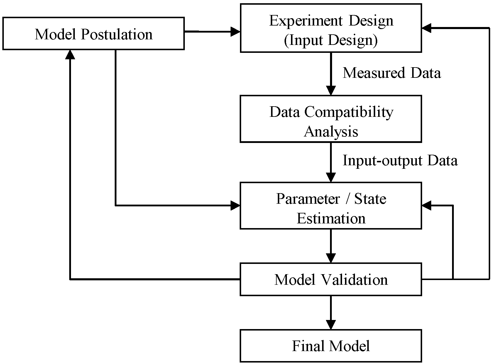
3. Aircraft System Identification
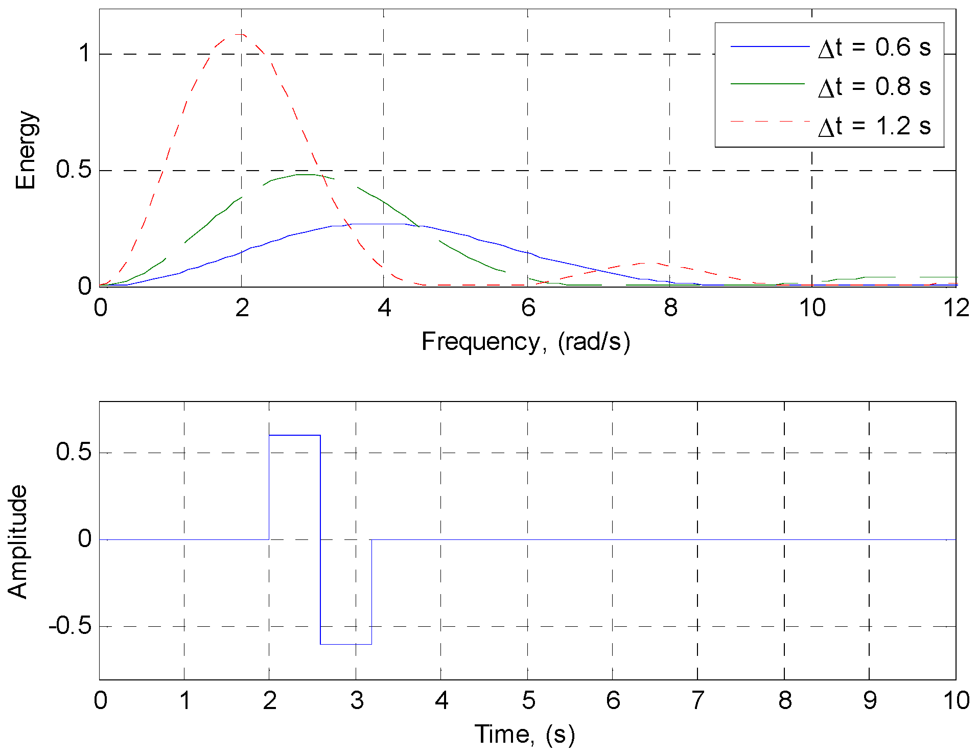
Aircraft system identification is the process of determining the unknown parameters of the adequate mathematical model [22], and the parameters have to be determined indirectly from the measured data. The flow chart of system identification process is presented in Figure 1. It begins with aircraft model postulation based on a priori knowledge about aircraft dynamic, aerodynamic and energy. After that, experiments are designed to measure the necessary output variables that are postulated. The experiment consists of deciding the operating flight conditions of the aircraft and designing of aircraft optimal control input to excite the dynamic motion of the aircraft. Next, the measured data undergo data compatibility analysis to compare with the reconstructed aircraft responses based on known rigid body kinematics. With the available input–output data, the parameters of the model can be estimated. The final step will be model validation with different set of input–output data. The identified model must demonstrate that its parameters have physically reasonable values and acceptable accuracy and that the model has good prediction capability on comparable aircraft maneuvers [23].

3.1. Input Design

The objective of input design for aircraft system identification is to excite the aircraft so that the data contain sufficient information for accurate modeling, subjected to the practical constraints of the experiment [23]. The common longitudinal flight maneuvers for aircraft system identification consist of short-period maneuver, phugoid maneuver, thrust variation, et cetera, which will be able to excite the longitudinal motion of aircraft, that is, short-period mode or phugoid motion. According to Jategaonkar [22], short-period motion is a fast responding longitudinal mode, provides the most information to enable the estimation of derivatives pertaining to the vertical and pitching motion. Since phugoid mode is the energy exchange, it is more suitable than short-period mode to excite the energy characteristic of the aircraft, which is the function of pitch angle, angle of attack, and longitudinal acceleration. The methods of utilizing the flight maneuvers in input design are called optimal input design, where the aircraft system identification uses the approach of a priori knowledge about the dynamic system response and the input is tailored accordingly. One of the popular optimal inputs is multistep input design where the range of aircraft natural frequencies are investigated, then followed by designing of suitable multistep input to cover the desired frequency range.
A more common multistep input is doublet input, as shown in Figure 2. The doublet input is a two-sided pulse, resulting with a symmetrical signal, which has higher energy and wider frequency bandwidth compared to pulse input. The time step of doublet input can be approximated by:
t DBLT = 1 2.7 ×   T osc
where ∆ t DBLT is the time step of doublet input and T osc is the period of aircraft oscillation.
The input design is a part of the iterative process of system identification, until an adequate model is developed and finally the model is successfully with the implementation of the controller. In this study, the energy distribution model consists of elevator input and total energy model consists of throttle input. For aircraft longitudinal motion, without significant influence from lateral dynamics, we can assume that energy distribution model is independent of total energy model. The suitable input for elevator is a doublet signal with ∆ t DBLT = 1 s. The maximum amplitude is eight degree and the minimum amplitude is −10 degree, as shown in Figure 3. The maximum positive elevator deflection is smaller to prevent the aircraft from excessive pitch down. The multi-steps input in the Figure 3 was suggested by Klein [23]. It is chosen due to the rich frequency spectrum covered in the input excitation which would result in better quality of dynamic response data.
The input of throttle is a pulse signal with ∆t = 3 s, as shown in Figure 4. The determination of the duration and magnitude for this input was based on the results of flight simulations and experiments. Moreover, in throttle response, there is a lag time constant, which is typically of the order of 2 to 3 s. This is the reason why the duration of 3 s is chosen for the input design of throttle.

3.2. Prediction Error Method (PEM)

In this study, PEM was applied to perform parameter estimation. According to Ljung [24], PEMs are a broad family of parameter estimation methods that can be applied to quite arbitrary model parameterizations and these methods have a close kinship with the maximum likelihood method. The state-space form of energy distribution is then readily available to be identified by using the PEM function in MATLAB System Identification Toolbox. The objective of system identification is to identify the discrete time state-space model in the following form:
x ( k + 1 ) = A x ( k ) + B u ( k ) + K w ( k )
y ( k ) = C x ( k ) + v ( k )
where k is the number of time-step. Note that x, y, u, w, and v are the state vector, output vector, input vector, process noise vector, and measurement noise vector, respectively. The remaining A, B, C, and K are the so-called system matrices, which determine the dynamics of the aircraft motion, and they are known to be constant with respect to a particular trimmed flight condition. Equation (21) is the output equation, and C is output matrix which represents the rationale of a linear relation between the state variables and the output. The used state vector, output vector, and input vector are presented as follows:
x = [ V   α   q   θ   a x   a z ] T
y = [ q   L ˙ ] T
u = [ δ e ]
The rationale of a linear relation between the state variables and the ∆ L ˙ is based on that the ∆ L ˙ is the function of the longitudinal acceleration and the flight path angle, and the flight path angle is the function of the pitch angle and angle of attack. In Equation (23), ∆q was selected to be the output state instead of ∆θ since ∆q is equal to ∆ θ ˙ and can be directly measured from the inertial sensor.
The predictor used to compute the one-step-ahead prediction for an underlying system description is the Kalman filter provided that w and v are Gaussian process. The predictor form of state-space representation can be given by:
x ^ ( k + 1 , ξ ) = A ( ξ ) x ^ ( k , ξ ) + B ( ξ ) u ( k , ξ ) + K ( ξ ) [ y ( k ) C ( ξ ) x ^ ( k , ξ ) ] y ^ ( k | ξ ) = C ( ξ ) x ^ ( k , ξ )
where x ^ and y ^ are the predicted states and predicted outputs, respectively, and ξ is a vector of parameters that typically correspond to unknown values of physical coefficients. The prediction error, ε, is given by:
ε ( k , ξ ) = y ( k ) y ^ ( k | ξ )
One of the approaches to qualify how small the ε is to form a scalar value norm or criterion function that measures the size of N. Consider a set of N data from an aircraft is given by:
Z N = [ y ( 1 ) , u ( 1 ) , y ( 2 ) , u ( 2 ) ,   ,   y ( N ) ,   u ( N ) ]
The corresponding norm:
V N ( ξ , Z N ) = 1 N k = 1 N || ε ( k , ξ ) || 2
Thus, the essence of PEM is the estimation of ξ from the model parameterization and ZN so that the norm VN is minimized.

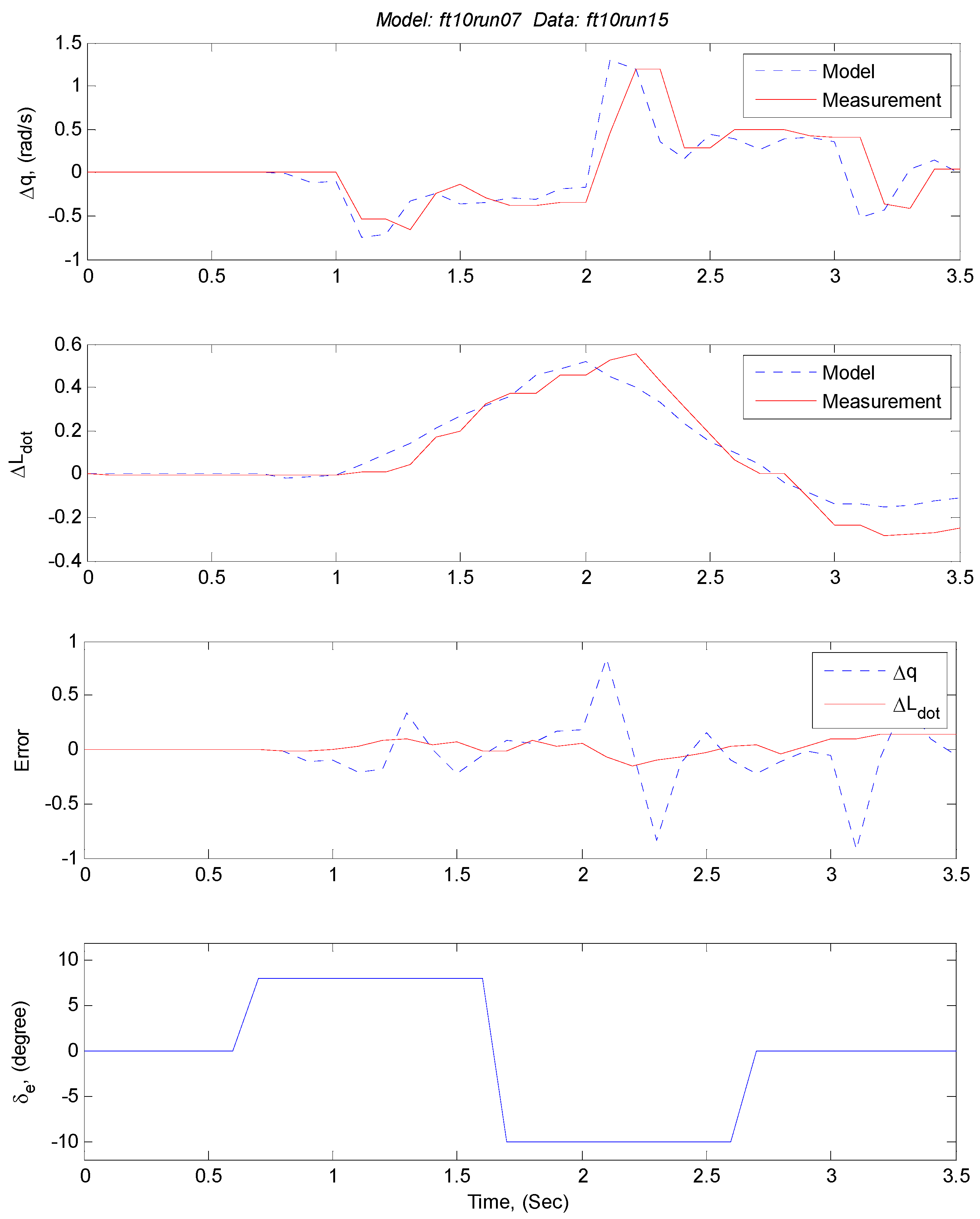
3.3. Aircraft Model Evaluation Method

In order to choose the best model among the identified models, it is required to apply a model evaluation method to evaluate the performance of the models. The used method in this study is adopted from Lee [18], which is variance accounted for (VAF) and norm. Given a set of N data, VAF is defined by the equation below:
V A F = { 1 var ( y i y ^ i ) var ( y i ) }   ×   100 % ,   i   =   1 ,   2 ,   3 ,   ,   N
where var(.) is the variance of the variable in the bracket, yi is the measured output, and y ^ i is the predicted output of the identified model. VAF is expressed in percentage where 100% means the outputs of identified model fit the measured output perfectly. However, there is a possibility to encounter with negative percentage, simply indicating that the outputs of the identified model do not fit the measured output. The norm is given by:
N R M = ( y ^ i y i y i ) T ( y ^ i y i y i ) ,   i   =   1 ,   2 ,   3 ,   , N
where a smaller value of norm will correspond to a better identified model.
There are total of 55 longitudinal flight data collected, performed by using elevator doublet input, with adequate elevator deflection angles. The flight data are named on the form as shown below for the ease of data management and analysis, as an example ft05run11 referred to the fifth flight test and the eleventh run. The aircraft distribution energy models were identified by imposing the performance requirements as shown below:
VAF ≥ 85% and NRM ≤ 15
The values of VAF have to be greater or equal to 85% and the norms must be smaller or equal to 15. There are total of 13 identified aircraft energy distribution models along with the trim conditions of the flight, VAF and norm. An example of an identified model ft11run10 that fulfills the performance requirements is shown in Figure 5. Identified models will be short-listed, and cross-validation is performed to further evaluate the performance of the model. Figure 6 presents the cross-validation result of model ft10run07 and data ft10run15. Cross-validation of model ft10run07 with other flight data is shown in Table 1. The discrete-time state-space of ft10run07 model, identified at trim airspeed of 27.44 m/s and altitude of 150.8 m, is given by Equations (20)–(24). From Figure 5, the VAF value of ∆q and L s ˙ are 92.31% and 94.52%, respectively, in which both values satisfy the minimum requirement of VAF at 85% based on the our experience.
Since model ft10run07 has better performance than others, it was adopted to be the model for control design. The identified discrete-time system matrices of model ft10run07 are shown below:
A = [ 0.8817 0.3071 0.1550 0.3277 0.1030 0.0179 0.1233 0.5893 0.1448 0.3950 0.4245 0.0658 0.1390 0.1834 0.5860 0.3802 0.8934 0.2023 0.3292 0.7071 0.3057 0.1676 0.0735 0.4707 0.0125 0.0863 0.5987 0.5262 0.1264 0.6399 0.1440 0.4595 0.0310 0.4682 0.5089 0.5017 ]
B = [ 0.0036 0.0049 0.0289 0.0523 0.0315 0.0173 ]
K = [ 0.0044 0.5807 0.1267 0.1459 0.1427 1.3377 0.1539 0.5222 0.0718 0.1018 0.3711 1.7641 ]
C = [ 0.6142 1.8588 0.2620 0.6264 0.4888 0.3138 1.2955 0.6276 0.1134 0.0499 0.0579 0.1528 ]

3.4. Total Energy Model

In Equation (18), the total energy is proportional to the deflection of throttle, ∆δT. The main objective for this section is to find out the relationship between ∆ E s ˙ and ∆δT, described by the parameter μ. The ∆ E s ˙ is obtained by applying the ∆δT as input with a time step of 3 s. An example of Pulse Width Modulation (PWM) input of ∆δT with a magnitude of 15 μ s is shown in Figure 7. We assume that the width of the input is proportional to the deflection of throttle. For each input with different magnitudes, five data were collected to obtain the average value of E s ˙ , as listed in Table 2. The average values of measured E s ˙ are plotted against the δ T , and the curve is fitted with a third degree polynomial, as shown in Figure 8. The slope of the fitted curve at zero PWM in Figure 8 is corresponding to the value of 0.0006522.

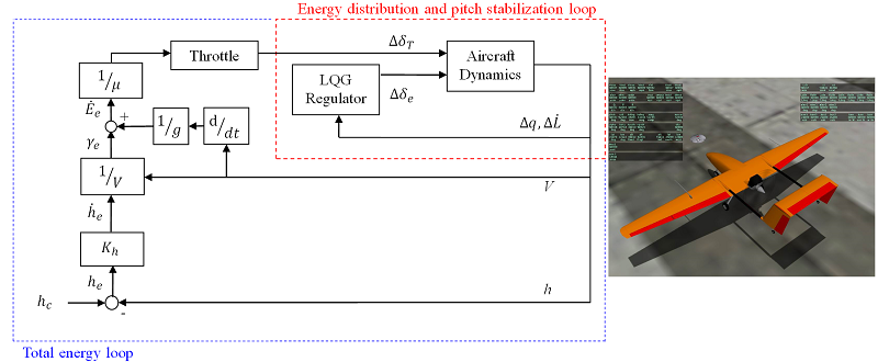
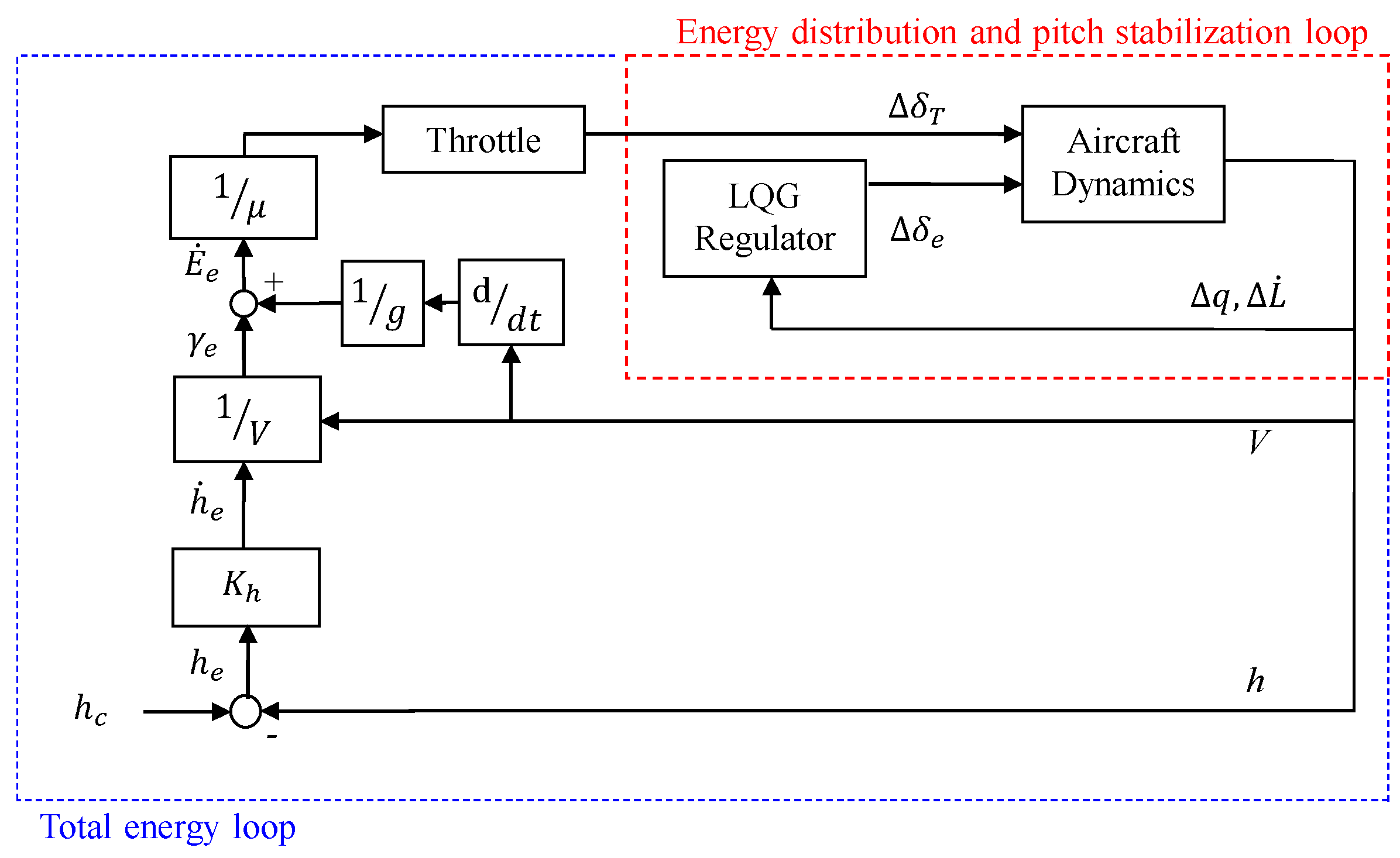
4. Optimal Energy Control System

4.1. OECS Design

In this study, an OECS has been proposed to form the aircraft longitudinal flight control system and to control the airspeed and altitude of the aircraft. There are two parameters, specific energy distribution rate, L ˙ s , and total specific energy rate, E ˙ s , utilized to characterize the energy of an aircraft or UAV. The block diagram of the proposed OECS is shown in Figure 9. The block diagram of the total energy loop is used to perform the tracking of aircraft altitude. Altitude tracking begins with the commanded altitude, h c . The difference between the commanded altitude and the current altitude of the aircraft, h, is the altitude error, h e which in turn will be scheduled by gains, K h . The values of K h were decided according to the tests of flight simulations. Table 3 shows the gains used in the gain scheduling. This simple gain scheduling is necessary to guarantee the throttle response is small, and thus meet the linearized total energy model, which stated that the increment of total specific energy rate, E ˙ e , is proportional to δ T . The result of gain scheduling is the climb rate or descent rate of an aircraft, which in turn will be divided by airspeed to obtain the flight path angle error, γ e . By assuming that the airspeed is almost constant, thus the longitudinal acceleration will be neglected.
The inner loop is energy distribution and pitch stabilization loop where the L ˙ s is regulated to zero. The inner loop, controlled by elevator, is responsible to distribute the energy of the aircraft between airspeed and altitude. The outer loop is total energy loop, which corresponds to the total energy of the aircraft. Total energy loop, controlled by throttle, is responsible to drive the total specific energy rate error E s ˙ to zero.

4.2. LQG Regulator

The objective of LQG regulator is to regulate L ˙ s and q to zero so that the aircraft’s energy is distributed among airspeed and altitude and the aircraft will achieve pitch-axis stabilization. This is completed by feeding the measured L ˙ s and q into the LQG regulator and the corresponding elevator command is computed. The design of LQG regulator is facilitated by the embedded functions in MATLAB. Eventually, a closed loop energy distribution state space model can be formed by using a series of functions in MATLAB. The process begins with the determination of optimal feedback gain of the regulator using the command dlqr. LQG regulator state-space model can be formed with the combination of Kalman estimator state-space model and LQR optimal feedback gain. For more details of LQG regulator design for a small UAV refer to studies [18,19].

5. Simulation Results and Discussion

In order to examine the feasibility and performance of the developed OECS, the simulations of OECS were conducted in the HIL system of Spoonbill UAV. Three flight maneuvers, level flight, descending, and climbing, were adopted to perform the simulations. Moreover, the influence of the wind effect was considered to validate the reliability of the developed system. The largest magnitude of wind was set to 8 m/s and the wind direction was set to be a headwind in the simulations.

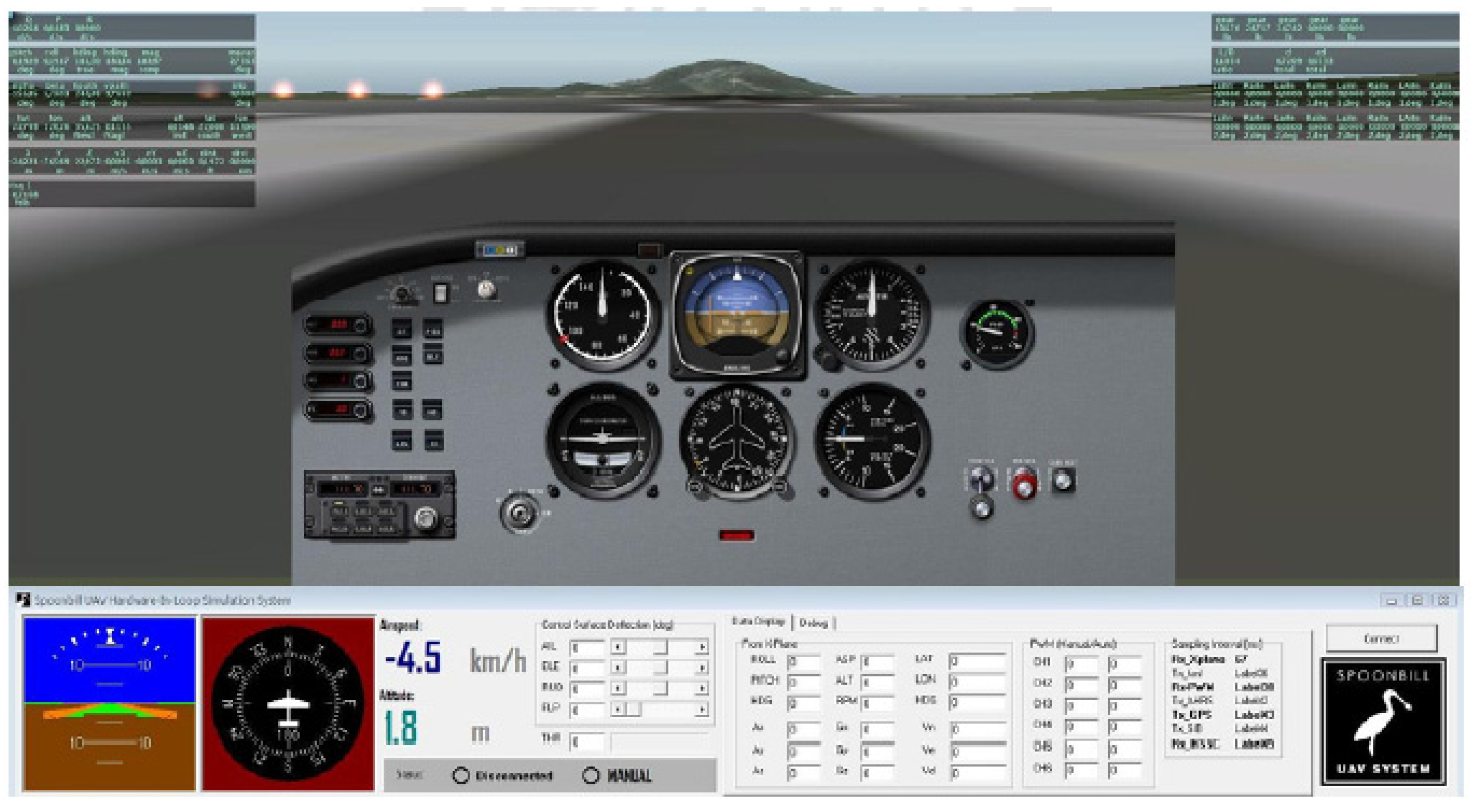
5.1. Hardware-in-the-Loop System of Spoonbill UAV

In order to validate the proposed OECS, a HIL system of Spoonbill UAV, as shown in Figure 10, was designed by integrating the onboard computer of Spoonbill UAV, a self-developed graphic user interface (GUI) program, and the X-Plane flight simulator, developed by Laminar Research. X-Plane can communicate with other applications via User Datagram Protocol (UDP). The GUI of the program, written using C++Builder (2007, Scotts Valley, CA, USA, 2007), is used to form the communication between the onboard computer and X-Plane Simulator. In the onboard computer, a flight program was used to integrate and save the flight data, and carry out the flight control at the rate of 20 Hz. Figure 11 shows the architecture of Spoonbill HIL system, and Figure 12 presents the communication between X-Plane and onboard computer with the help of GUI program.

5.2. Airspeed and Altitude Hold

With the help of HIL system, the developed OECS is first simulated in the aircraft level flight without the presence of wind. The simulation results of level flight, as shown in Figure 13, show that the change of pitch rate, q , is regulated within ± 0.01   rad / s and L ˙ s is regulated at 0.01. At the same time, the airspeed is maintained at around 20.8 m/s and the altitude shows agreement with the commanded altitude, h c , at 150 m.
Furthermore, aircraft level flight, as shown in Figure 14, is simulated with the presence of wind, and the largest magnitude of wind is 8 m/s. The results present that the change of pitch rate, q , is regulated within ± 0.10   rad / s and L ˙ s is regulated within 0.05. Moreover, the airspeed is regulated at trim airspeed of 20.3 m/s with the variation of ± 0.5   m / s . The trim airspeed is dependent on the identified aircraft energy distribution model. On the other hand, the altitude deviation is less than 2 m from the commanded altitude of 120 m. As a summary for level flight, the performance of the OECS satisfies the airspeed and altitude is successfully held.

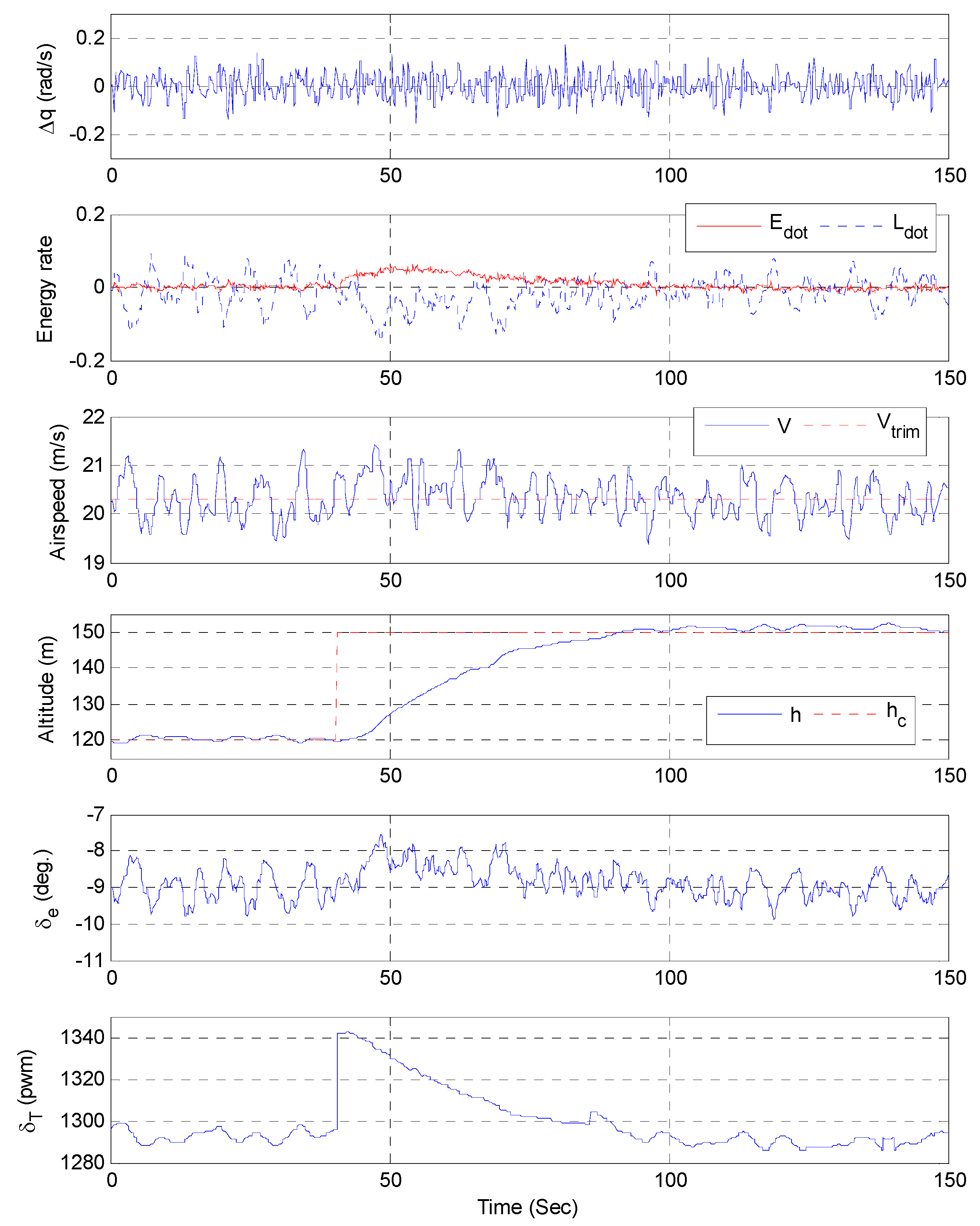
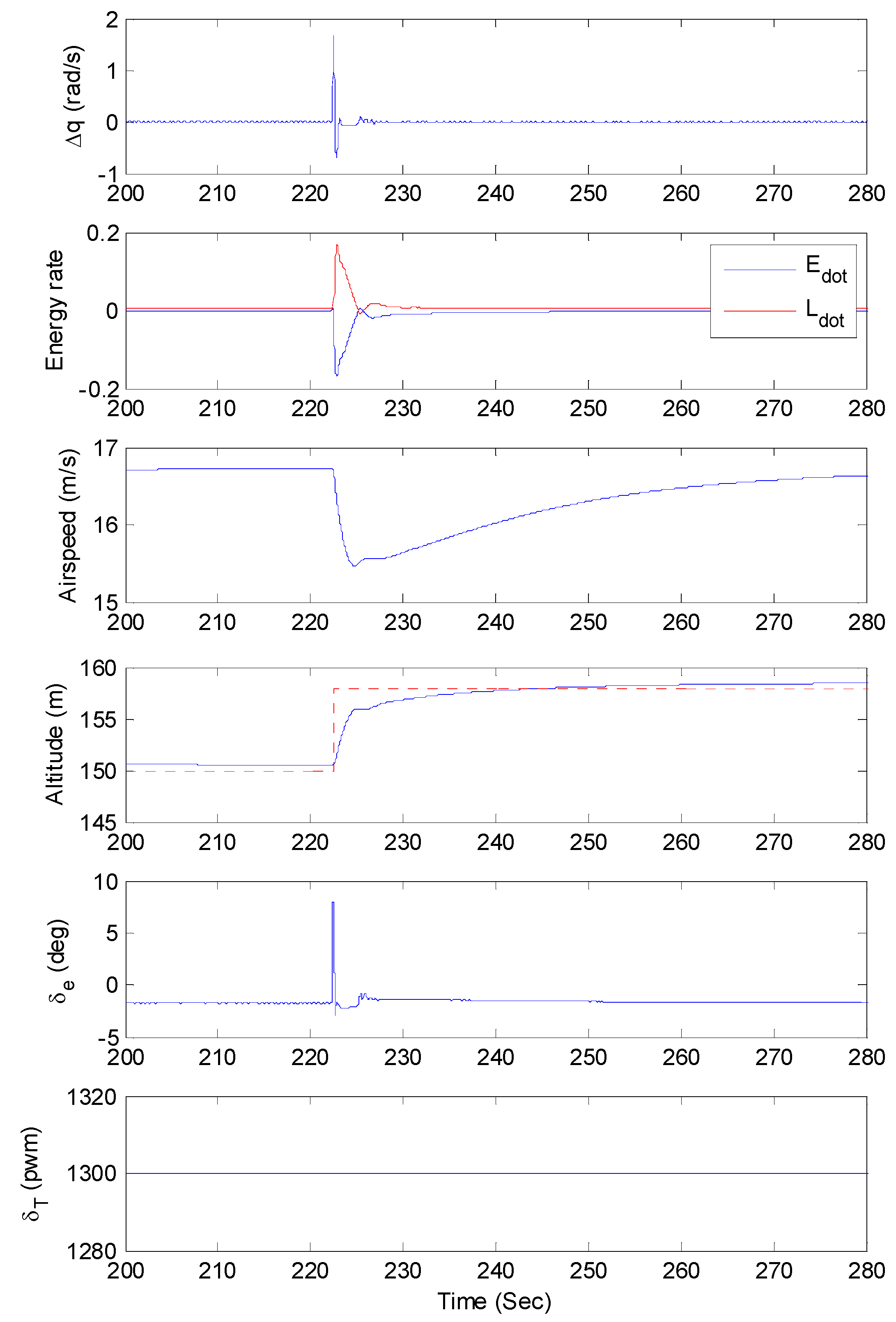
5.3. Climbing Maneuver

This section presents the climbing performance of the aircraft with and without the presence of wind. The climbing maneuver was performed at the trim airspeed of 20.8 m/s, without the presence of wind. The simulation results are shown in Figure 15. The initial altitude is 150 m and the commanded altitude is 158 m. During the aircraft climbing, the airspeed is maintained within the variation of ± 0.2   m / s from trim airspeed. The settling time for the climbing maneuver is around 40 s. Moreover, the change of pitch rate, q , is regulated within ± 0.01   rad / s , which is the same as in level flight. On the other hand, L ˙ s is regulated around the neighborhood of 0.01. Note that there is a slight decrease of L ˙ s at 18th second, which corresponds to the increase in flight path angle of the aircraft.
Figure 16 shows the simulation results with the presence of wind and the largest magnitude of wind is 8 m/s throughout the climbing maneuver. During the aircraft climbing, the change of pitch rate, q , is regulated within ±   0.15   rad / s and L ˙ s is regulated within the variation of ± 0.1 . Besides that, the airspeed is maintained at trim airspeed within the variation of ± 1   m / s . The settling time of altitude tracking is around 65 s.

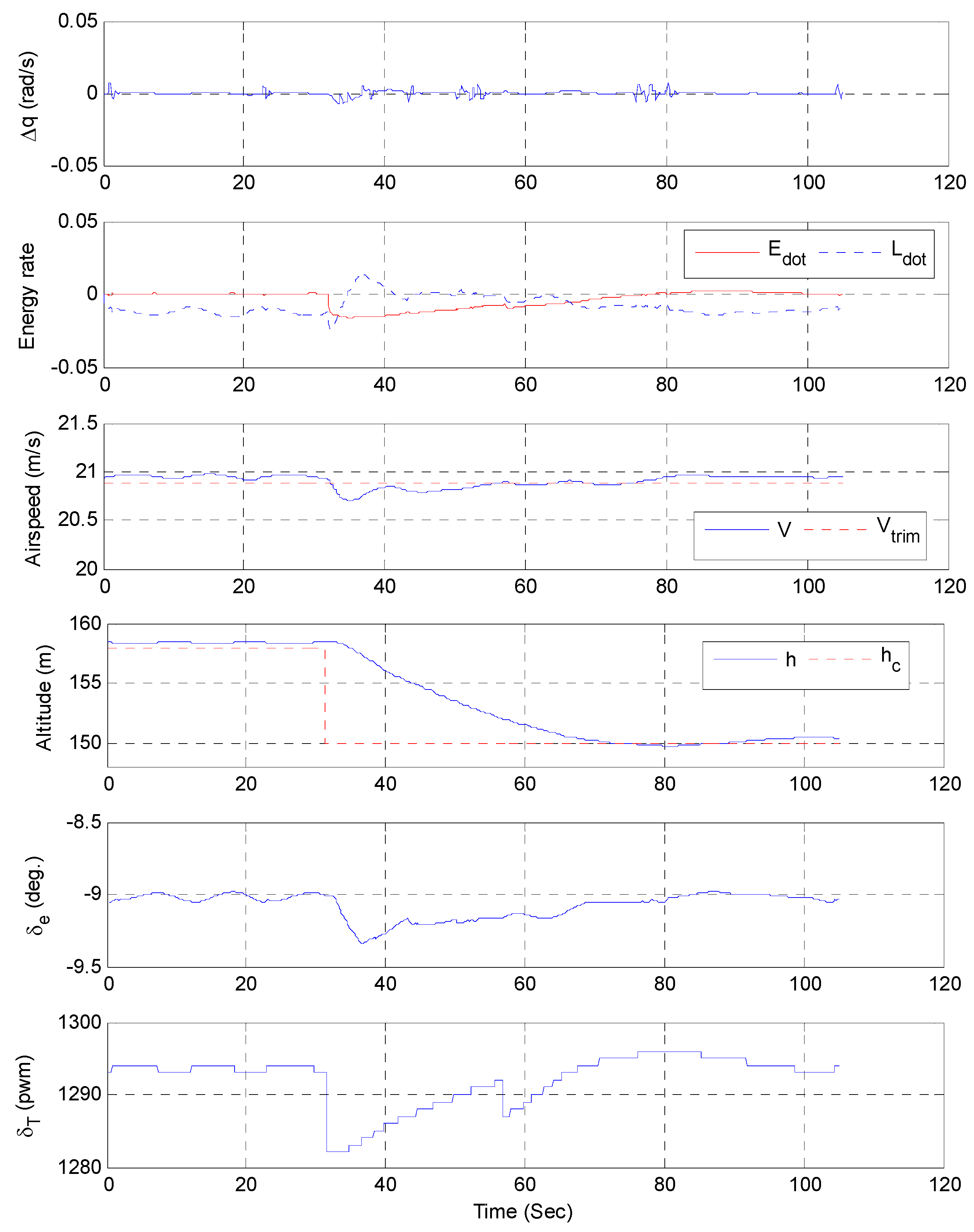
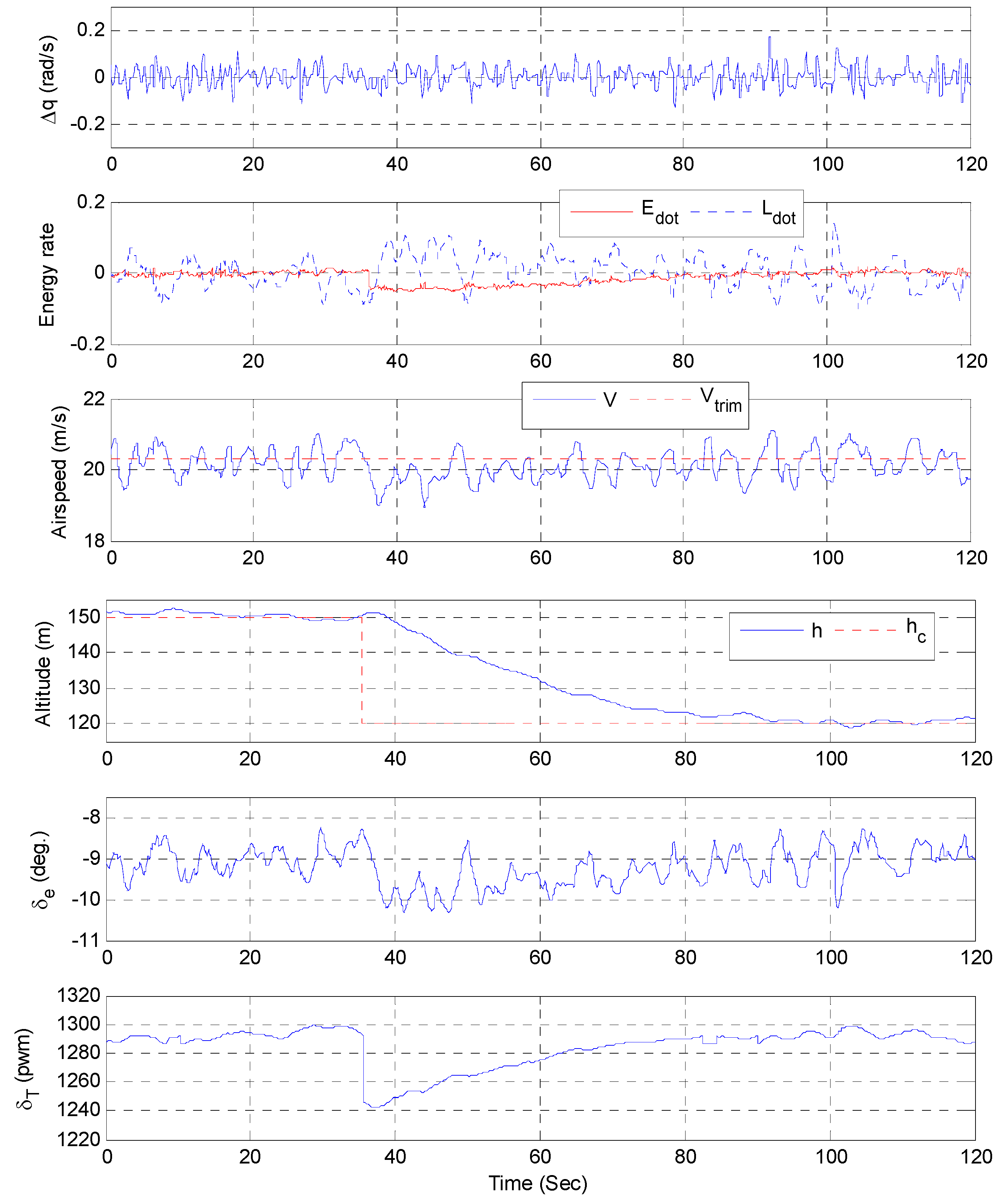
5.4. Descent Maneuver

For the descent maneuver, the simulation result without the presence of the wind is shown in Figure 17. Both the change of pitch rate, q , and L ˙ s are regulated within ± 0.01   rad / s and ± 0.02 , respectively. The aircraft descended from 158 to 150 m in around 40 s, while maintaining the airspeed within ± 0.2   m / s from trim airspeed. For the simulation results of aircraft descend with the presence of wind, as shown in Figure 18, the errors of q , L ˙ s , airspeed, altitude, and altitude tracking settling time are almost the same as the aircraft climb maneuver.

5.5. Result Comparison of OECS with Fuzzy Logic Control

To compare the performance and fuel efficacy of the proposed OECS with other controller, a flight controller based on Fuzzy logic control was used in this study. The developed OECS is a model-based method, which means that it requires the system identification process and identified model to design the control system. In contrast to the model-based method, Fuzzy logic control (FLC) is a knowledge-based method, which means that no model is constructed, and the design of the FLC requires some understanding of the plant’s behavior and expert’s experience. The details of the adopted FLC autopilot refer to the study in [25].
Both of the climbing and descending performance of the target UAV without the presence of wind was evaluated. Since there is no autothrottle system in the used FLC, the throttle of the FLC was set to be constant and its value was 1300 PWM. The simulation results of climbing maneuver are shown in Figure 19. The initial altitude is 150 m and the commanded altitude is 158 m. During the aircraft climbing, the airspeed decreases dramatically about 0.8 m/s from initial airspeed. The settling time for the climbing maneuver is around 30 s, and the maximum change of pitch rate, ∆q, is about 1.5 rad/s. When the climbing maneuver is performed, the energy rates change dramatically. The simulation results of descending maneuver are shown in Figure 20. The results are similar to that of the climbing maneuver. In contrast to the OECS, the climbing and descending performance and fuel efficiency of the proposed OECS are better than that of FLC. The aircraft is maintained approximately at trim airspeed, and the required throttle is lower than that in FLC. Moreover, the energy rates are more stable and within small values. The results show that the proposed OECS can achieve the goal of the optimization of the fuel consumption.

5.6. Summary of OECS Performance

Table 4 presents a summary of OECS performance for different flight maneuvers and flight conditions. The simulation results for aircraft level flight, descending, and climbing maneuvers show that the errors of airspeed and altitude are very small in windless condition. Besides that, the q and L ˙ s are successfully regulated to a value close to zero. The errors with the presence of wind are acceptable for aircraft level flight, descending, and climbing maneuvers. Moreover, the settling time for climbing and descending maneuvers is the same for tracking a similar altitude difference. This shows that the linearity of the total energy model is satisfied. Furthermore, by comparing the simulation results of OECS and FLC, it shows that the proposed OECS has better performance and fuel efficiency than that of FLC.

6. Conclusions

The design and implementation of the proposed OECS, which is based on the total energy of an aircraft, has been presented in this study. OECS is an aircraft longitudinal flight control system which is based on pilot-like control strategy to control the airspeed and altitude of the aircraft. The controller design process begins with the postulation of the aircraft model, from aircraft equations of motion and energy equations. After that, the postulated model was identified using the system identification method. The identified models were used to design the developed OECS. Finally, OECS was verified in HIL system of Spoonbill UAV. Three flight maneuvers, level flight, descending, and climbing, were adopted to perform the simulations. In addition, the influence of the wind effect was considered to validate the reliability of the developed system. The largest magnitude of wind was set to 8 m/s. The simulation results show that the implementation of the proposed OECS for different flight maneuvers and flight conditions was successfully validated in the HIL simulation system of the used UAV. When comparing the performance and fuel efficiency of the proposed OECS with another flight control system based on Fuzzy logic control, the results show that the proposed OECS has better performance and fuel efficiency than that of FLC.

Acknowledgments

This study was supported by the Ministry of Science and Technology of Taiwan under grant number MOST 103-2632-E-035-001-MY3 and MOST 104-2622-E-035-019-CC3. Furthermore, this study was directed by Fei-Bin Hsiao, who passed away in February 2014. The authors admire and respect him for his great contributions to aerospace societies in the world.

Author Contributions

Ying-Chih Lai determined the research framework, proposed the main idea, and performed mathematical modeling. Wen Ong Ting performed the implementation of the developed algorithm and simulations.

Conflicts of Interest

The authors declare no conflict of interest.

References

  1. Chen, S.-W.; Chen, P.-C.; Yang, C.-D.; Jeng, Y.-F. Total energy control system for helicopter flight/propulsion integrated controller design. J. Guid. Control Dyn. 2007, 30, 1030–1039. [Google Scholar] [CrossRef]
  2. Denker, J.S. See How It Flies. Available online: http://www.av8n.com/how/ (accessed on 18 November 2016).
  3. Lambregts, A. Integrated system design for flight and propulsion control using total energy principles. In Proceedings of the American Institute of Aeronautics and Astronautics, Aircraft Design, Systems and Technology Meeting, Fort Worth, TX, USA, 17–19 October 1983.
  4. Lambregts, A.A. Vertical flight path and speed control autopilot design using total energy principles. AIAA Pap. 1983. [Google Scholar] [CrossRef]
  5. Akmeliawati, R.; Mareels, I.M.Y. Nonlinear energy-based control method for aircraft automatic landing systems. IEEE Trans. Control Syst. Technol. 2010, 18, 871–884. [Google Scholar] [CrossRef]
  6. Kaminer, I.; O’Shaughnessy, P. Integration of four-dimensional guidance with total energy control system. J. Guid. Control Dyn. 1991, 14, 564–573. [Google Scholar] [CrossRef]
  7. Wu, S.-F.; Guo, S.-F. Optimum flight trajectory guidance based on total energy control of aircraft. J. Guid. Control Dyn. 1994, 17, 291–296. [Google Scholar] [CrossRef]
  8. Warren, A. Application of total energy control for high-performance aircraft vertical transitions. J. Guid. Control Dyn. 1991, 14, 447–452. [Google Scholar] [CrossRef]
  9. Voth, C.; Ly, U.-L. Design of a total energy control autopilot using constrained parameter optimization. J. Guid. Control Dyn. 1991, 14, 927–935. [Google Scholar] [CrossRef]
  10. Bruce, K.; Kelly, J.R.; Person, J.R.L. NASA B737 flight test results of the total energy control system. In Proceedings of the Astrodynamics Conference, Williamsburg, VA, USA, 18–20 August 1986; American Institute of Aeronautics and Astronautics: Reston, VA, USA, 1986. [Google Scholar]
  11. Rzucidlo, P. TECS/THCS based flight control system for general aviation. In Proceedings of the AIAA Modeling and Simulation Technologies Conference, Chicage, IL, USA, 10–13 August 2009.
  12. Lamp, M.; Luckner, R. The total energy control concept for a motor glider. In Advances in Aerospace Guidance, Navigation and Control; Springer: Heidelberg, Germany, 2013; pp. 483–502. [Google Scholar]
  13. Kale, A.; Singhz, G.; Patel, V. 1-adaptive-output feedback based energy control. In Proceedings of the 2015 European Control Conference (ECC), Linz, Austria, 15–17 July 2015; IEEE: New York, NY, USA, 2015; pp. 2792–2797. [Google Scholar]
  14. Brigido-González, J.; Rodríguez-Cortés, H. Experimental validation of an adaptive total energy control system strategy for the longitudinal dynamics of a fixed-wing aircraft. J. Aerosp. Eng. 2015, 29, 04015024. [Google Scholar] [CrossRef]
  15. Weiss, S.; Siegwart, R. Real-time metric state estimation for modular vision-inertial systems. In Proceedings of the 2011 IEEE International Conference on Robotics and Automation (ICRA), Shanghai, China, 9–13 May 2011; IEEE: New York, NY, USA; pp. 4531–4537.
  16. Deittert, M.; Richards, A.; Toomer, C.; Pipe, A. Dynamic soaring flight in turbulence. In Proceedings of the AIAA Guidance, Navigation and Control Conference, Chicago, IL, USA, 10–13 August 2009; pp. 2–5.
  17. Akhtar, N.; Whidborne, J.F.; Cooke, A.K. Real-Time Trajectory Generation Technique for Dynamic Soaring UAVs; Department of Aerospace Sciences, Cranfield University: Oxfordshire, UK, 2008. [Google Scholar]
  18. Lee, C.; Chan, W.; Jan, S.; Hsiao, F. A linear-quadratic-gaussian approach for automatic flight control of fixed-wing unmanned air vehicles. Aeronaut. J. 2011, 115, 29–41. [Google Scholar] [CrossRef]
  19. Lee, C.-S.; Hsiao, F.-B.; Jan, S.-S. Design and implementation of linear-quadratic-gaussian stability augmentation autopilot for unmanned air vehicle. Aeronaut. J. 2009, 113, 275–290. [Google Scholar] [CrossRef]
  20. Rugh, W.J.; Shamma, J.S. Research on gain scheduling. Automatica 2000, 36, 1401–1425. [Google Scholar] [CrossRef]
  21. Hsiao, F.-B.; Hsieh, S.-Y.; Chan, W.-L.; Lai, Y.-C. Engine speed and velocity controller development for small unmanned aerial vehicle. J. Aircr. 2008, 45, 725–728. [Google Scholar] [CrossRef]
  22. Jategaonkar, R. Flight Vehicle System Identification: A Time Domain Methodology; AIAA: Reston, VA, USA, 2006; Volume 216. [Google Scholar]
  23. Klein, V.; Morelli, E.A. Aircraft System Identification: Theory and Practice; American Institute of Aeronautics and Astronautics: Reston, VA, USA, 2006. [Google Scholar]
  24. Ljung, L. Prediction error estimation methods. Circuits Syst. Signal Process. 2002, 21, 11–21. [Google Scholar] [CrossRef]
  25. Lai, Y.C.; Hsiao, F.B. Application of fuzzy logic controller and pseudo-attitude to the autonomous flight of an unmanned aerial vehicle. J. Chin. Inst. Eng. 2010, 33, 387–396. [Google Scholar] [CrossRef]
Figure 1. Flow chart of system identification process.
Applsci 06 00369 g001
Figure 2. Doublet input with different time steps.
Applsci 06 00369 g002
Figure 3. Elevator doublet with time step of 1 s as input.
Applsci 06 00369 g003
Figure 4. Thrust pulse with time step of 3 s as input.
Applsci 06 00369 g004
Figure 5. An example of identified model ft11run10.
Applsci 06 00369 g005
Figure 6. Model ft10run07 cross-validated with data ft10run15.
Applsci 06 00369 g006
Figure 7. The response of the E s ˙ with an increment of throttle input.
Applsci 06 00369 g007
Figure 8. Curve fit relation of E s ˙ and δ T .
Applsci 06 00369 g008
Figure 9. The block diagram of the proposed OECS. OECS, optimal energy control system; LQG, linear-quadratic-Gaussian.
Applsci 06 00369 g009
Figure 10. Spoonbill unmanned aerial vehicle (UAV) in X-Plane flight simulator.
Applsci 06 00369 g010
Figure 11. Architecture of Spoonbill HIL system. HIL, hard-in-the-loop; COM, communication port; PWM, Pulse Width Modulation; RC, radio control; AHRS, attitude and heading reference system; GPS, Global Positioning System; UDP, User Datagram Protocol.
Applsci 06 00369 g011
Figure 12. Communication between X-Plane and onboard computer with the help of GUI program. GUI, graphic user interface.
Applsci 06 00369 g012
Figure 13. Simulation results of level flight without the presence of wind.
Applsci 06 00369 g013
Figure 14. Simulation results of level flight with the presence of wind.
Applsci 06 00369 g014
Figure 15. Simulation results of climbing without the presence of wind.
Applsci 06 00369 g015
Figure 16. Simulation results of climbing with the presence of wind.
Applsci 06 00369 g016
Figure 17. Simulation results of descending without the presence of wind.
Applsci 06 00369 g017
Figure 18. Simulation results of descending with the presence of wind.
Applsci 06 00369 g018
Figure 19. Fuzzy logic control (FLC) simulation results of climbing without the presence of wind.
Applsci 06 00369 g019
Figure 20. FLC simulation results of descending without the presence of wind.
Applsci 06 00369 g020aApplsci 06 00369 g020b
Table 1. Cross-validation of model ft10run07 with other flight data. VAF, variance accounted for; NRM, norm.
Model V (m/s)h (m)VAF (%)NRM
q L ˙ q L ˙
ft09run0627.03151.066.9985.376.098.58
ft09run0726.50153.467.1293.577.227.48
ft10run0129.33150.578.1291.999.279.84
ft10run0228.43150.775.5492.447.997.21
ft10run0727.44150.8----
ft10run1428.35151.557.9886.563.854.77
ft10run1529.10150.654.5291.905.365.85
ft10run1728.73150.265.0594.135.335.61
ft10run2128.80151.089.5694.825.376.48
ft11run0727.98150.758.9287.655.903.88
ft11run1027.65150.871.7584.848.637.51
ft11run2528.40151.076.1691.032.976.07
ft11run2829.25156.789.4990.874.684.05
Table 2. The average value of E s ˙ from positive throttle input. PWM, Pulse Width Modulation.
δ T ( P W M ) = 15
Flight Tests V (m/s)h (m) E s ˙
ft33run1030.0150.50.0050
ft33run1130.2152.60.0045
ft33run1230.0150.70.0050
ft33run1330.0151.00.0050
ft33run1430.1153.00.0050
Average--0.0049
Table 3. The gains used in the gain scheduling.
No. h e = | h c h | K h
1 0 h e 2 0.130
2 2 < h e 5 0.045
3 5 < h e 10 0.025
4 h e > 10 0.008
Table 4. A summary of OECS performance for different flight maneuvers and flight conditions.
ConditionWindlessWind
ManeuverLevelClimbDescendLevelClimbDescend
Altitude Tracking (m)150150→158158→150150120→150150→120
Settling Time (s)-4040-6565
q (rad/s)0.010.010.010.150.150.15
L ˙ s 0.010.010.010.050.100.10
Altitude Deviation (m)0.200.200.202.002.002.00
Airspeed Deviation (m/s)0.100.200.200.501.001.00

