A Physically—Based Geometry Model for Transport Distance Estimation of Rainfall-Eroded Soil Sediment

Abstract

Estimations of rainfall-induced soil erosion are mostly derived from the weight of sediment measured in natural runoff. The transport distance of eroded soil is important for evaluating landscape evolution but is difficult to estimate, mainly because it cannot be linked directly to the eroded sediment weight. The volume of eroded soil is easier to calculate visually using popular imaging tools, which can aid in estimating the transport distance of eroded soil through geometry relationships. In this study, we present a straightforward geometry model to predict the maximum sediment transport distance incurred by rainfall events of various intensity and duration. In order to verify our geometry prediction model, a series of experiments are reported in the form of a sediment volume. The results show that cumulative rainfall has a linear relationship with the total volume of eroded soil. The geometry model can accurately estimate the maximum transport distance of eroded soil by cumulative rainfall, with a low root-mean-square error (4.7–4.8) and a strong linear correlation (0.74–0.86).

1. Introduction

Surface transport distance of sediment is an important consideration when evaluating and predicting sediment transportation and landscape evolution resulting from rainfall-induced soil erosion in mountainous regions. The process chronologically includes (1) precipitation producing the runoff and related soil detachment; (2) the eroded soil accumulating as sediment and related maximum transport distance. For the runoff and soil erosion rate, widely used prediction models include: (1) a model based on real statistic data like the Universal Soil Loss Equation (USLE), composed of six factors to predict average annual soil weight [1,2]; (2) a physical mechanism-based model such as the Water Erosion Prediction Project (WEPP) model, which is capable of predicting spatial and temporal distributions of soil detachment and deposition, both for single rainfall events or on a continuous basis, on both small (hill slopes, roads, small parcels) and large (watershed) scales [3]; (3) the European Soil Erosion Model (EUROSEM) model, a dynamic distributed model able to simulate sediment transport, erosion, and deposition by rill and inter-rill processes in single storms for both individual fields and small catchments [4]; and (4) the Kinematic Runoff and Erosion Model (KINEROS) model, which is an event-oriented, physically based model describing the processes of interception, infiltration, surface runoff, and erosion from agricultural and urban watersheds [5]. For the eroded soil sediment and related transport distance, two approaches are typically used to describe transport: (1) considering complex physical equations or (2) empirical coefficients. (1) For example, Limburg Soil Erosion Model (LISEM) is a physically based, hydrological, and soil erosion model for simulating the hydrology and sediment transport during and immediately after a single rainfall event applied in an agricultural catchment of a size ranging from 1 hectare up to approximately 100 km² [6]; Bennett [7] provides three equations that describe the movement of suspended sediment particles in a one-dimensional, infinitely wide, free-surface flow. The first two equations describe the continuity of mass and momentum in the flow of water. The third describes the conservation of mass for sediment transport. Unfortunately, this model involves seven parameters that are not easily obtained. (2) An exponential transport-distance model (as used by Wainwright et al. [8]) is used to simulate splash. Routing of splash is described in the four cardinal directions away from the source point, with relative weightings for upslope and downslope movement. Widespread overland flow is simulated using an exponential distribution parameterized by the calculated median travel distance. Although these data only relate to relatively coarse particle sizes, Parsons et al. [9] find that they adequately predict rates of movement of finer particles. Sediment distribution and deposition follow the spatial pattern of the flow-routing algorithm directly. Concentrated flows are simulated with an exponential distribution function parameterized using the median transport distances, based on the review of available data by Hassan et al. [10]. It should be noted that this equation is based on the ordinary regression results of Hassan et al. [10], rather than the functional relationship form. These equations are relatively simple but some parameters, particularly those involving energy, are not easily estimated. In addition, the transport distance of soil particles of a particular size, not whole sediment mass, is the output in these equations. Since these models require many parameters and are relatively complex, here we use a simple fitting equation to link the rainfall events and soil erosion. Based on this fitting equation, we develop a straightforward soil erosion transport–distance model in which a geometric relationship is used to predict the maximum transport distance of soil erosion. Some physical experiments validate our physically based geometry model, providing meaningful results while using minimal historical data [11,12].

2. Methods

We used a flume with field soil to simulate the surface layer of a representative hillslope. Four nozzles were employed to simulate the different intense rainfall events. Sensors in the soil layer collected the hydrological data at time increments. The volumes of eroded soil under different intense rainfall events were calculated using the imaging tool at each time step. These experimental results of sediment volumes were input to validate a geometry-based model for predicting the maximum transport distance of eroded soil.

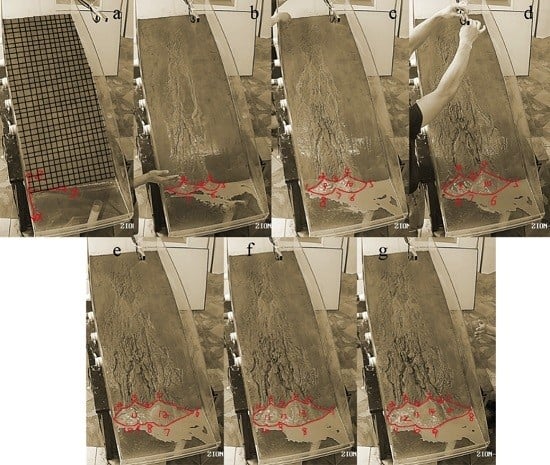
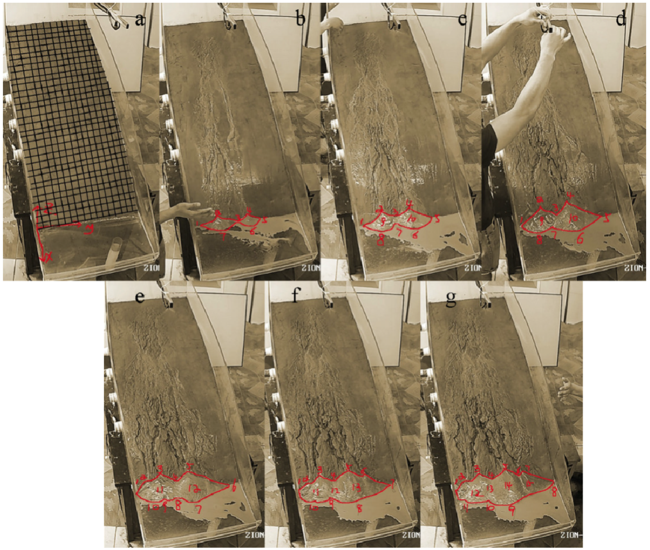
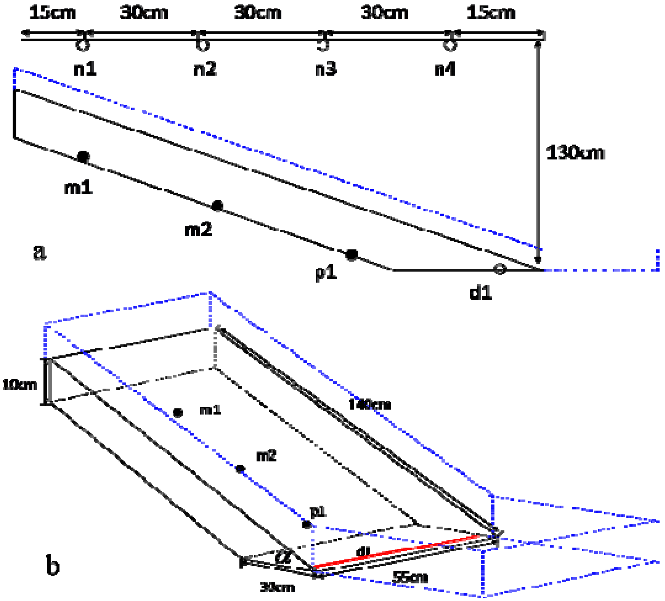
2.1. Physical Modeling and Monitoring Devices

A surface soil layer of Fengdu Mountain, close to the Yangtze River Bank, Chongqing, China was reproduced in a flume. The surface soil of Fengdu Mountain can be easily eroded under heavy rainfall (particle-size distribution curve in Figure 1). Fengdu Mountain is located at the Three Gorges Reservoir Area, where the average annual rainfall is 1074.6 mm and 70% of the annual rainfall occurs between May and September [13]. The average annual erosion rate is 2087 t/km² in Yangtze River Basin [14]. Soil properties were tested in the laboratory and consisted of quaternary eluvial material, clay, and silty clay. A model slope was constructed in a flume device made of Plexiglas (the blue dotted line in Figure 2 is the flume) with an area of 8250 cm² (length is 140 cm and width is 55 cm). A 10 cm deep layer simulates the real shallow layer of the hill and, furthermore, is convenient for installing the sensors for the hydrological investigation. The slope inclination is ~26°, close to that observed in the field [13]. A plate squeezed the soil layer with a force of 120 N to form the slope. In order to reduce the “boundary effect,” we used a covering of polytetrafluoroethylene (PTFE) (friction coefficient is 0.04) on both sides of the flume. In Figure 2, two moisture transducers (Model number DS200, Beijing Dingtek Technology Corp., Ltd, Beijing, China) (frequency domain sensors: measuring range 0%–100%, resolution 0.1%, deviation ±2% with a soil contact area of less than 20 mm²) and one pore water pressure transducer (Model number CYY2, Xi’an Weizheng Technology Corp., Ltd, Xi’an, China) (diameter 3 cm, height 1.6 cm, measuring range ±10 kPa, deviation ±0.2%) are installed at three different positions along the hillslope; d1 is a drainage ditch (55 × 3 cm) for calculation of the subsurface drainage. One high-definition digital camera is used to record images of the sediments in the front view (another camera helps to estimate the height of the sediment from side view). A water-pump supplies water resources through four nozzles (uniformity coefficient is 0.91) for rainfall simulation. A flow meter between pump and nozzles controls the rainfall intensity (10–250 mL/min). Rain fall is introduced in a series of six rainfall events, each with a constant rainfall duration (we took pictures every minute for six minutes) and with different intensity levels of approximately 15, 25, 35, 45, 55 and 65 mm/h, respectively (15 mm/h is close to the threshold of soil erosion and 65 mm/h is the maximum value achievable using the device). By approximately minute seven (under 65 mm/h rainfall intensity) and minute eight (under 55 mm/h rainfall intensity), progressive landslide failure occurs at the foot of the slope (this occurs in such a short time because of the high initial water content in the slope). This carries soil sediment away and could incur error in the volume calculations. Thus, a maximum time of six minutes ensures soil erosion without sediment loss. For every minute of six intense rainfall events, we took a measurement of eroded soil sediment volume (a total of 36 measurements and 29 eroded soil sediments were observed). For each test, we totally reconstructed the slope model and gave a pre-added rainfall (15 mm/h) for 1 h. After a 3 h interval, the experiment began. Each test was conducted under similar initial conditions of geometry, material, moisture content, and pore water pressure (PWP) (deviation ±3%). Initial water content was relatively high in order to shorten the experiment time.

Figure 1. Particle-size distribution curve (Natural cohesion is 3.4 kPa, Phi is 32° compared to saturated cohesion 0.1 kPa and Phi 28.4°; the natural and saturated densities are 1.83 and 2.05 g/cm³).

Figure 1. Particle-size distribution curve (Natural cohesion is 3.4 kPa, Phi is 32° compared to saturated cohesion 0.1 kPa and Phi 28.4°; the natural and saturated densities are 1.83 and 2.05 g/cm³).

Figure 2. Physical slope model: (a) side view and (b) stereoscopic view, where n1, n2, n3 and n4 are nozzles for rainfall; m1 and m2 are moisture transducers; p1 is the pore water pressure transducer; d1 is drainage ditch; and $\alpha$ is ~26°.

Figure 2. Physical slope model: (a) side view and (b) stereoscopic view, where n1, n2, n3 and n4 are nozzles for rainfall; m1 and m2 are moisture transducers; p1 is the pore water pressure transducer; d1 is drainage ditch; and $\alpha$ is ~26°.

2.2. Calculations of Sediment Volume

In Figure 3, video footage in the front of the slope was used to identify the coordinates of eroded soil for transport estimations. A basic grid network and coordinate system were set up. Under time domains, approximately every seven centimeters, we drew a point along the edge of the soil sediment. Every peak in the sediment must be identified in this way. In the Y-direction (positive and negative), two cameras permitted estimation of the height of the sediment (peak value). Erosion characteristics from the video images were extracted in the form of coordinates after video grid analysis. Calculation of sediment is as shown in Figure 4. Specifically, considering the two different images (current and original digital elevation model (DEM), for example, Figure 5a,b), we used seven time steps to extract a 3D point cloud for every minute. Then, based on this, we developed different digital elevation models by the Kriging gridding interpolation using Golden Surfer 9.0 (Golden Software Inc., Golden, CO., US, 2009), which is a full-function 3D visualization, contouring, and surface-modeling package. The software includes an extensive variogram modeling subsystem, and we chose the linear variogram model [15]. Finally, as the difference between original and current DEM (Figure 5c), based on these models, we estimated the volume of sediment deposition. Extraction of coordinates owes some variances to the real value (~4%) and lens distortions, and the distance between camera and ground affects the accuracy of the picture area (~4.2%) [12].

Figure 3. Sediment volume under 25 mm/h at (a) 0 min, (b) 1 min, (c) 2 min, (d) 3 min, (e) 4 min, (f) 5 min, (g) 6 min.

Figure 3. Sediment volume under 25 mm/h at (a) 0 min, (b) 1 min, (c) 2 min, (d) 3 min, (e) 4 min, (f) 5 min, (g) 6 min.

Figure 4. The principle of sediment volume calculation. The red area is the initial slope part and the blue area is the sediment volume.

Figure 4. The principle of sediment volume calculation. The red area is the initial slope part and the blue area is the sediment volume.

Figure 5. Sediment volume calculation by Golden Surfer (at 2 min under 25 mm/h rainfall intensity): (a) whole volume (sediment volume + initial slope volume); (b) initial slope volume; (c) using the whole volume to reduce the initial slope volume.

Figure 5. Sediment volume calculation by Golden Surfer (at 2 min under 25 mm/h rainfall intensity): (a) whole volume (sediment volume + initial slope volume); (b) initial slope volume; (c) using the whole volume to reduce the initial slope volume.

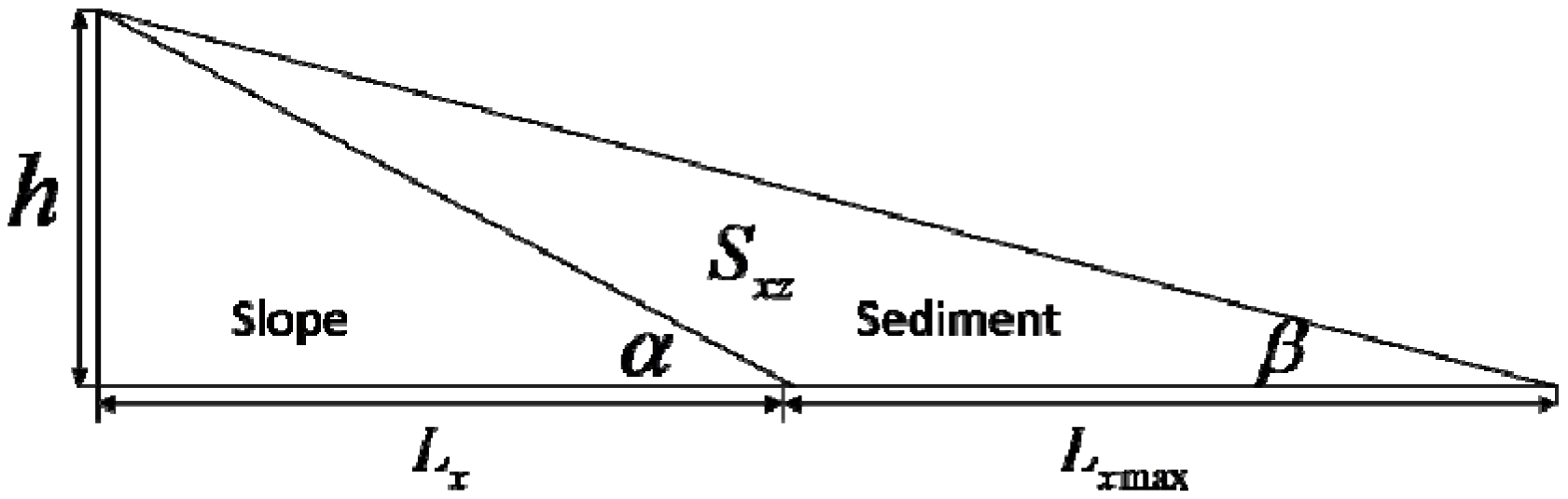
2.3. Geometry Model for the Eroded Soil Maximum Transport Distance

2.3.1. Maximum Transport Distance

Based on our experimental results, we developed a geometry model to estimate the sediment’s maximum transport distance. The main inputs of our geometry prediction model are cumulative rainfall and sediment angle, while the output is maximum transport distance. Figure 6 is a vertical topographic view of eroded sediment (e.g., sediment in Figure 5 in the Z-direction), where: $L_{x\max }$ is the maximum distance of debris sediment in the X-direction; $L_x\prime$ is the length of vertical shadow of sediment area; X = 0 is the edge line of the initial slope toe; and $L_y$ is the width of soil sediment.

Figure 6. Vertical topographic view of eroded sediment (at 5 min under 25 mm/h rainfall intensity).

Figure 6. Vertical topographic view of eroded sediment (at 5 min under 25 mm/h rainfall intensity).

2.3.2. Geometry Model for Sediment Maximum Transport Distance

Figure 7 describes the geometric relationship between the eroded sediment and the slope. We inferred a geometric relation between the maximum transport distance ($L_{x\max }$) and area ($S_{xz}$).

Figure 7. Lateral view of eroded soil sediment (debris).

Figure 7. Lateral view of eroded soil sediment (debris).

The processes are as follows:

$$S_{xz}=L_{x\max }h/2$$

(1)

$$h=\tan \alpha L_x=\tan \beta (L_{x\max }+L_x)$$

(2)

$$S_{xz}=L_{x\max }{L}_x\tan \alpha /2$$

(3)

$$L_x=L_{x\max }\tan \beta /(\tan \alpha -\tan \beta )$$

(4)

$$S_{xz}={L_{x\max }}^2\tan \beta \tan \alpha /2(\tan \alpha -\tan \beta ),$$

(5)

where $S_{xz}$ is the lateral area; $h$ is the height of debris; $L_{x\max }$ is the maximum transport distance (here, we consider all the $L_{x\max }$ to be in the Y-direction in the same time domain); $L_x$ is the length of the sediment shadow minus the $L_{x\max }$; $\alpha$ is the angle of the slope; and $\beta$ is the angle of sediment.

In Figure 6, we consider the volume element $\Delta V^i$ in the Y-direction to equate to the $S_{xz}$ times $\Delta {L_y}^i$ element. The whole volume of sediment is shown in Equation (9).

$$\Delta V^i=S_{xz}\Delta {L_y}^i$$

(6)

$${\displaystyle \sum _1^i\Delta V^i}={\displaystyle \sum _1^i{S}_{xz}\Delta {L_y}^i}=S_{xz}{L}_y$$

(7)

Putting Equation (5) into Equation (7) provides Equation (8) as follows:

$$V=S_{xz}{L}_y={L_{x\max }}^2\tan \beta \tan \alpha /2(\tan \alpha -\tan \beta )L_y$$

(8)

$$L_{x\max }=(2V(\tan \alpha -\tan \beta )/\tan \beta \tan \alpha L_y{)}^{1/2}$$

(9)

The model boundaries limit the rate of sediment transport in the direction $L_y$. Thus, $L_{x\max }(t)$ is bigger than $L_{y\max }(t)$. Another issue is that, in order to reduce calculation complexity, $S_{xz}(t)$ and $\beta (t)$ in the $L_y$ direction are approximated to be the same for each time domain.

2.4. Model Fit and Validation

We performed a simple regression analysis to fit the cumulative rainfall and eroded soil sediment volume. The root mean square error (RMSE), the sum of squared errors of prediction (SSE), and scatter correlation analysis are used to evaluate the geometry model prediction. The sum of squared errors of prediction (SSE) is a measure of the discrepancy between the data and the estimated values from a model. A small SSE indicates a tight fit of the model to the data [16]. R-square indicates how well the data points fit a statistical model [17]. The root mean square error (RMSE) is a frequently used measure of the differences between the values predicted by a model or an estimator and the values actually observed [18]. The p-value < 0.01 indicates significant correlation.

3. Results

3.1. Sediment Yield Volumes under Rainfall Events

Figure 8a displays PWP evolution with time under different rainfall intensities. At the first minute, PWP increases rapidly in part because of surface water runoff concentration at the foot of the slope. High simulated rainfall intensities in our experiments result in the rapid appearance of surface water runoff. Figure 8b,c display moisture content at the top and middle of the slope, respectively. Apparently, the initial moisture content at the middle of the slope is higher than that at the top of the slope. Also, the moisture content at the middle of the slope increases faster compared with the moisture content at the top.

Figure 8. Hydrological monitoring data: (a) p1, (b) m1 and (c) m2.

Figure 8. Hydrological monitoring data: (a) p1, (b) m1 and (c) m2.

Total soil sediment yield increases with rainfall duration for each intensity sequence. Similarly, at the same time step sediment, yield increases with rainfall intensity. Under 15 mm/h rainfall intensity, no soil loss occurred and thus there was no sediment data. Figure 9a shows a 3D curve of rainfall intensity, rainfall duration, and sediment. Figure 9b shows the 3D vertical view between rainfall intensity, duration, and sediment. Table 1 lists two potential fitted equations: (1) considering rainfall intensity and duration affecting the sediment separately, and (2) considering cumulative rainfall affecting the sediment. (An obvious linear relationship is observed.)

Figure 9. 3D fitting curve (rainfall intensity (mm/h), rainfall duration (min), and sediment (e-3m³). (a) Optimum 3D fitting curve; (b) shadow map of optimum 3D fitting curve.

Figure 9. 3D fitting curve (rainfall intensity (mm/h), rainfall duration (min), and sediment (e-3m³). (a) Optimum 3D fitting curve; (b) shadow map of optimum 3D fitting curve.

Table 1. Fitted equations (x = rainfall duration > 0 min, y = rainfall intensity > 15 mm/h).

Label	Fitted Equation	SSE (m3)	R-Square	RMSE (m3)	p-Value
1	(ax + by) + c	0.0001378	0.7936	0.0007281	<0.01
2	a(xy) + b	0.0003277	0.9509	0.0003484	<0.01

Table 1. Fitted equations (x = rainfall duration > 0 min, y = rainfall intensity > 15 mm/h).

Label	Fitted Equation	SSE (m3)	R-Square	RMSE (m3)	p-Value
1	(ax + by) + c	0.0001378	0.7936	0.0007281	<0.01
2	a(xy) + b	0.0003277	0.9509	0.0003484	<0.01

Percentage of erosion can describe how much soil is eroded by the rainfall events in a certain area by percentage. Percentage of erosion (E) should follow the equations: E = 0.013((ax + by) + c) × 100% or E = 0.013 (a(xy) + b) × 100%.

As shown in Table 1, the governing equation between cumulative rainfall and volume of eroded soil sediment is linear, as follows:

$$(I-r)S_l\cdot t=a_{1}V$$

(10)

$$R-R_r=a_{2}V$$

(11)

where I is the rainfall intensity; r is the rainfall intensity threshold of sediment movement; S_l is the rainfall area; V is the volume of eroded sediment in time t; t is the rainfall time; a₁ and a₂ are coefficients required by fitting the experimental data; and R and R_r are the cumulative rainfall and cumulative rainfall threshold of the initial sediment, respectively.

Taking Equation (11) into Equation (9) in order to link the rainfall produces:

$$L_{x\max }={(2(R-R_r)(\tan \alpha -\tan \beta )/a_2\tan \beta \tan \alpha L_y)}^{1/2}$$

(12)

Considering the time domain, Equation (13) constructs the link between rainfall and maximum transport distance as follows:

$$L_{x\max }(t)={(2(R(t)-R_r)(\tan \alpha -\tan \beta (t))/a_2\tan \beta (t)\tan \alpha L_y(t))}^{1/2}$$

(13)

3.2. Geometry Model for the Eroded Soil Transport Distance

Twenty-nine effective experimental results of eroded soil volumes were input into the geometry model for maximum transport distance. The correspondingly observed transport distances are used for comparisons. Figure 10a displays the comparison between physical experiment measurements and model predictions. Figure 10b displays the results of the error analysis of the model prediction by linear relation and RMSE calculation.

Figure 10. Model performance: (a) measurement versus prediction of the model (n = 29); (b) linear relationship between model and measurement (RMSE = 4.8) (n = 29).

Figure 10. Model performance: (a) measurement versus prediction of the model (n = 29); (b) linear relationship between model and measurement (RMSE = 4.8) (n = 29).

4. Discussion

4.1. Rainfall Producing Yield Soil Sediment

High soil water content increases sediment detachability by runoff shear forces and raindrop impact [19]. It is therefore because of the high initial soil moisture content that we observe soil erosion in the first minute of our experiments. In Figure 8a, p1 shows positive value indicating that saturated soil or runoff was produced. Since the strength of the soil is reduced, shearing the soil by surface water flow is easier. Figure 3 illustrates that the slope toe is more heavily eroded than other parts of the slope. The moisture content of soil in a particular area depends on the inflow and outflow of water. In Figure 8b, m1 at the top of the slope does not receive runoff from other parts of the slope and subsequently displays a slow increase in moisture content, consistent with the rainfall intensity increment (no more than 0.2%). Initial moisture could also affect the moisture content. When the initial soil moisture is low, water fills the soil pore space more quickly than it drains out (due to a high suction hold on the water). By contrast, in soil with high moisture content, the drainage rate is high and there is a balance between water inflow and outflow. As shown in Figure 8b,c, at m2 the moisture improves more than 0.5% compared to at m1.For one thing, it is likely due to runoff supply from the upper slope to the middle part of the slope. For another, since the water flows downward, the subsurface water flow from m1 to m2 can also increase the moisture of m2.

High rainfall intensity and the subsequent increase in surface runoff increase the rate of soil erosion [3]. In our experiments, no eroded sediment is produced when the rainfall intensity is lower than 15 mm/h. Sediment yields are linked to transport and detachment capacity, which is the limiting factor of the erosion process. If the detachment capacity is significantly lower than the transport capacity, the process is referred to as “detachment-limited erosion” [20]. Materials are transported only after being detached; therefore, there must be a threshold rainfall amount at which soil erosion will begin. Indeed, several modeling studies observed that shearing force induced by runoff must overcome resistance in order to achieve soil loss [5,21]. In Figure 9b the soil erosion rate increases with time (when the rainfall intensity is smaller than 50 mm/h; it decreases with time when the rainfall intensity is greater than 50 mm/h). In terms of rainfall intensity, the soil erosion rate in the first three minutes is greater than in the last three minutes. Decreasing soil erosion rates with time could be a result of the subsurface soil’s appearance after the surface soil detachment. The previous subsurface becomes the new surface soil, which can store more water. Another important factor is the formation of concentrated flows; this increases erosion in the rills but reduces runoff from other parts, which may result in flows with high sediment concentration, close to the limit of transport capacity. Importantly, the cumulative rainfall is linearly related to the yield sediment volume, with high correlation (Table 1, label 2). In order to explore the linear relationship between rainfall and soil erosion over a wider range, 147 random instances of cumulated rainfall and eroded volume (interpolated data extracted from the experimental data) acquired from physical experiments were reproduced by a trace linear interpolation model (linear interpolation produces the samples between neighbor cumulative rainfall events and the samples between corresponding soil erosions volumes in the meantime). Figure 11a shows the comparison between random samples and the linear model fitting. Figure 11b displays the linear relationship between measurement (random samples) and the model fitting.

Figure 11. The linear model (cumulative rainfall and eroded soil sediment): (a) random samples versus model fitting (n = 147); (b) linear relationship between random samples and model fitting (RMSE = 1.2623) (n = 147).

Figure 11. The linear model (cumulative rainfall and eroded soil sediment): (a) random samples versus model fitting (n = 147); (b) linear relationship between random samples and model fitting (RMSE = 1.2623) (n = 147).

4.2. Geometry-Based Model for the Transport Distance

The geometric model proposed here, as well as predicting rainfall-induced soil erosion, can also incorporate previous rainfall-soil erosion relationships to estimate the maximum transport distance. In order to assess the predictive capability of the model over a wider data range, 147 random instances of cumulative rainfall and maximum transport distance were identified from physical experiments (linear interpolation produces the samples between neighbor cumulative rainfall events and the samples between corresponding maximum transport distance in the meantime). Figure 12a displays the random samples against the model prediction. Figure 12b shows the relationship between the random samples and the model prediction and presents the associated error (RMSE = 4.7).

Figure 12. Error analysis of model prediction: (a) random samples versus model prediction (n = 147); (b) linear relationship between model prediction and random samples (RMSE = 4.7) (n = 147).

Figure 12. Error analysis of model prediction: (a) random samples versus model prediction (n = 147); (b) linear relationship between model prediction and random samples (RMSE = 4.7) (n = 147).

In our study, the flexible and straightforward model depends on three inputs—cumulative rainfall, slope angle, and debris angle. The sediment angle may be uncertain and easily affected by rainfall (Figure 13). The histogram of sediment angles is as shown in Figure 14. Most sediment angles were found to range between 18° and 22° (very close to the residual friction angle of 21°), which means that a coefficient, such as residual friction angle, could arguably be used as a substitute. The significance of using a coefficient is that it can reduce the inputs to cumulative rainfall and slope angle, which could be more straightforward.

Figure 13. Cumulative rainfall with sediment angle. (a) Sediment angle with cumulative rainfall (n = 29) based on physical tests; (b) sediment angle with cumulative rainfall (n = 147) based on random field.

Figure 13. Cumulative rainfall with sediment angle. (a) Sediment angle with cumulative rainfall (n = 29) based on physical tests; (b) sediment angle with cumulative rainfall (n = 147) based on random field.

Figure 14. Frequency of sediment angle: (a) histogram based on physical test (n = 29); (b) histogram based on random field (n = 147).

Figure 14. Frequency of sediment angle: (a) histogram based on physical test (n = 29); (b) histogram based on random field (n = 147).

4.3. Limitations and Suggestions for Future Study

Due to the cost and time-intensive nature of the experiments described in this study, we did not consider vegetation cover, the effect of slope, and soil material variability. Slope shape and surface roughness design was a relatively simple representation that minimized dimension effects; however, this is common for any mini-physical model experiment [22]. In our study, any dimension effect arises mainly from the underestimated rainfall impact and the “boundary effect.” A covering of PTFE (friction coefficient is 0.04) was installed on both sides of the flume in order to reduce the “boundary effect.” In the future, the impact of the slope effect and coupled rainfall, slope, and material effects on soil erosion could be our next research direction.

5. Conclusions

This study investigated to what extent different rainfall intensities and durations affect the maximum transport distance of eroded sediment using a physical simulation experiment in a flume. The physical experiment simulated rainfall-induced surface soil erosion events. The hydrological monitoring data, sediment yield volumes under rainfall events, and the eroded soil transport distance were measured or calculated. Meanwhile, a geometry-based model was developed to evaluate the maximum transport distance of rainfall-eroded soil sediment. Based on these results, our understandings and conclusions areas as follows:

Firstly, the pore water pressure (PWP) and moisture content in different positions of the slope are influenced greatly by the rainfall intensities and durations. At the first minute, PWP increases rapidly in the toe part because of surface water runoff concentration at the foot of the slope. The moisture content at the soil layer is characterized by slow growth. The moisture content at the middle of the slope increases faster compared with the moisture content at the top. Furthermore, high intensive rainfall events result in the rapid appearance of surface water runoff.

Secondly, total soil sediment yield increases with rainfall duration for each intensity sequence, and at the same time step sediment yield increases with rainfall intensity. Moreover, under time domains soil erosion volume linearly relates to cumulative rainfall. Soil erosion volume can be estimated using two fitted equations: (1) considering rainfall intensity and duration affecting the sediment separately, and (2) cumulative rainfall affecting the sediment. The former has a R-square of 0.79 and a RMSE of 0.00073 m³ and the latter has a R-square of 0.95 and a RMSE of 0.00035 m³.

Thirdly, based on the linear relationship of soil erosion volume and cumulative rainfall obtained from the experimental results, a geometry-based model for calculating the maximum transport distance ($L_{x\max }$) is developed using just three parameters: cumulative rainfall, slope angle, and debris angle. The cumulative rainfall and slope angle may be obtained by consulting local hydrological and geological data. The debris angle may use the resident friction angle. According to the experimental results, this flexible and straightforward soil erosion transport distance model can predict maximum transport distance with low error.

References

1. Wischmeier, W.H.; Smith, D.D. Predicting rainfall erosion losses. In USDA Agricultural Handbook; U.S. Department of Agriculture: Washington, DC, USA, 1978. [Google Scholar]
2. Renard, K.G.; Foster, G.R.; Weesies, G.A.; McCool, D.K.; Yoder, D.C. Predicting soil erosion by water: A guide to conservation planning with the Revised Universal Soil Loss Equation RUSLE. In Agriculture Handbook; U.S. Department of Agriculture: Washington, DC, USA, 1997. [Google Scholar]
3. Flanagan, D.C.; Nearing, M.A. USDA Water Erosion Prediction Project: Hillslope Profile and Watershed Model Documentation; USDA-ARS National Soil Erosion Research Laboratory: West Lafayette, IN, USA, 1995.
4. Morgan, R.P.C.; Quinton, J.N.; Smith, R.E.; Govers, G.; Poesen, J.W.A.; Auerswald, K.; Chisci, G.; Torri, D.; Styczen, M.E. The European Soil Erosion Model (EUROSEM): A dynamic approach for predicting sediment transport from fields and small catchments. Earth Surf. Process. Landf. 1998, 23, 527–544. [Google Scholar] [CrossRef]
5. Smith, R.E.; Goodrich, D.C.; Quinton, J.N. Dynamic, distributed simulation of watershed erosion: The KINEROS2 and EUROSEM models. J. Soil Water Conserv. 1995, 50, 517–520. [Google Scholar]
6. De Roo, A.P.J.; Wesseling, C.G.; Ritsema, C.J. LISEM: A single-event physically based hydrological and soil erosion model for drainage basins. I: Theory, input and output. Hydrol. Process. 1996, 10, 1107–1117. [Google Scholar] [CrossRef]
7. Bennett, J.P. Concepts of mathematical modelling of sediment yield. Water Resour. Res. 1974, 10, 485–492. [Google Scholar] [CrossRef]
8. Wainwright, J.; Parsons, A.J.; Abrahams, A.D. Field and computer simulation experiments on the formation of desert pavement. Earth Surf. Process. Landf. 1999, 24, 1025–1037. [Google Scholar] [CrossRef]
9. Parsons, A.J.; Wainwright, J.; Powell, M.; Kaduk, J.D.; Brazier, R.E. A conceptual model for determining soil erosion by water. Earth Surf. Process. Landf. 2004, 29, 1293–1302. [Google Scholar] [CrossRef]
10. Hassan, M.; Church, M.; Ashworth, P.J. Virtual rate and mean distance of travel of individual clasts in gravel-bed channels. Earth Surf. Process. Landf. 1992, 17, 617–627. [Google Scholar] [CrossRef]
11. Schmidt, J. (Ed.) Soil Erosion: Application of Physically Based Models; Springer Science & Business Media: Berlin, Germany, 2013.
12. Nie, W.; Huang, R.Q.; Zhang, Q.G.; Xian, W.; Xu, F.L.; Chen, L. Prediction of experimental rainfall-eroded soil area based on S-shaped growth curve model framework. Appl. Sci. 2015, 5, 157–173. [Google Scholar] [CrossRef]
13. Rong, B.A.I. Stability analysis and control to Mingshan Landslide of Fengdu in the Three Gorges Reservoir Area. J. Lanzhou Railw. Inst. 2002. (In Chinese) [Google Scholar] [CrossRef]
14. Fan, J.; Liu, F.; Guo, F.; Zhang, H. Soil erosion assessment and cause analysis in three gorges reservoir area based on remote sensing. J. Mt. Sci. 2011, 39, 306–311. (In Chinese) [Google Scholar]
15. Fencík, R.; Vajsáblová, M. Parameters of interpolation methods of creation of digital model of landscape. In Proceedings of the 9th AGILE Conference on Geographic Information Science, Visegrád, Hungary, 20–22 April 2006.
16. Draper, N.R.; Smith, H. Applied Regression Analysis, 3rd ed.; John Wiley: New York, NY, USA, 1998. [Google Scholar]
17. Steel, R.G.D.; Torrie, J.H. Principles and Procedures of Statistics with Special Reference to the Biological Sciences; McGraw Hill: New York, NY, USA, 1960; pp. 187–287. [Google Scholar]
18. Hyndman, R.J.; Koehler, A.B. Another look at measures of forecast accuracy. Int. J. Forecast. 2006. [Google Scholar] [CrossRef]
19. Römkens, M.J.; Helming, K.; Prasad, S.N. Soil erosion under different rainfall intensities, surface roughness, and soil water regimes. Catena 2002, 46, 103–123. [Google Scholar] [CrossRef]
20. Van Rompaey, A.; Bazzoffi, P.; Jones, R.J.; Montanarella, L. Modeling sediment yields in Italian catchments. Geomorphology 2005, 65, 157–169. [Google Scholar] [CrossRef] [Green Version]
21. Bathurst, J.C.; Wicks, J.M.; O’Connell, P.E. The SHE/SHESED basin scale water flow and sediment transport modelling system. In Computer Models of Watershed Hydrology; Singh, V.P., Ed.; Water Resource Publication: Highlands Ranch, CO, USA, 1995; pp. 563–594. [Google Scholar]
22. Upton, J.G.G.; Fingleton, B. Spatial Data Analysis by Example. Volume 1: Point Pattern and Quantitative Data; Wiley: Chichester, UK, 1985. [Google Scholar]