Article

Dynamically Determining the Toll Plaza Capacity by Monitoring Approaching Traffic Conditions in Real-Time

1
Department of Civil and Environmental Engineering, Seoul National University, Seoul 151-744, Korea
2
School of Civil, Architectural and Environmental Engineering, Korea University, Seoul 136-713, Korea
3
California Department of Transportation, Operations, Oakland, CA 94612, USA
*
Authors to whom correspondence should be addressed.
Appl. Sci. 2016, 6(3), 87; https://doi.org/10.3390/app6030087
Submission received: 4 January 2016 / Revised: 4 March 2016 / Accepted: 9 March 2016 / Published: 18 March 2016

Abstract

:
This study presents an analytical method for dynamically adjusting toll plaza capacity to cope with a sudden shift in demand. The proposed method uses a proxy measure developed using discharge rate observed at toll plazas and segment travel times measured by probe vehicles. The effectiveness of the method has been evaluated by analyzing the empirical data obtained from toll plazas in the San Francisco Bay Area before and after toll plaza capacity changed. Findings indicate that the estimated number of vehicles stored near the upstream of toll plaza based on discharge rate and their travel times can be used as a proxy measure for predicting the effect of changes in toll plaza capacity. The proposed model can aid government agencies to dynamically adjust the toll plaza capacity in response to a sudden shift in demand due to various situations of failure.

1. Introduction

Toll plaza staffing schedules at seven bridges (see Figure 1) in the San Francisco Bay Area were recently revised to better allocate resources to address traffic demand. These schedule revisions accompanied changes in the number of cash and FasTrak lanes at the toll plazas. Currently, drivers using the FasTrak lane are required to pay the toll through use of an electronic transponder installed on the vehicle, while drivers using the cash lane can pay either with cash or via the electronic transponder. Due to these changes, the traffic near two bridges experienced delays while those at other bridge locations remained unchanged. Under normal operation, dynamically changing toll plaza capacity might be unnecessary. However, during the closure of a major freeway corridor due to construction or catastrophic failure, there may be a sudden shift in demand for alternate routes. This sudden shift in demand, coupled with limited government resources, may necessitate dynamically determining toll plaza operations. To this end, this study presents an analytical method for dynamically adjusting toll plaza capacity based on real-time demand and reports on the validity of the proposed method which has been evaluated using empirical data.
Edie [1] was one of the first studies to utilize empirical data to investigate the relationship among flows, number of toll booths, and level of service. Based on findings from analyzing data at the Lincoln Tunnel, he proposed a method for determining the number of toll booths required and recommended toll collectors′ schedules. Recent studies have primarily relied on simulated data; Burris and Hildebrand, Astarita et al., and Al-Deek developed a microscopic simulation model to evaluate toll plaza systems [2,3,4,5,6]. Researchers focused on evaluating both the performance of each toll lane, and the entire system using commercial microscopic simulation software including MODSIM, Paramics, and VISSIM [7,8,9,10]. A toll plaza simulation model, SHAKER, was recently developed to determine the hourly maximum capacity with different lane types [11,12]. Wander and Peirce formulated a model to optimize staffing at toll plazas through investigation of traffic parameters at a border checkpoint [13]. This model compared wage costs for staff with border waiting times for travelers.
One of the main challenges in implementing the findings from these simulation studies is that the data needed to implement the proposed strategies are often lacking in practice: Often, loop detectors in the field are not located at strategic locations and may be non-existent in the vicinity of toll plazas. To address this issue, this paper proposes a proxy measure for dynamically determining toll plaza capacity based on discharge rate at the toll plazas and segment travel times detected by probe vehicle.

2. Description of the Study Site

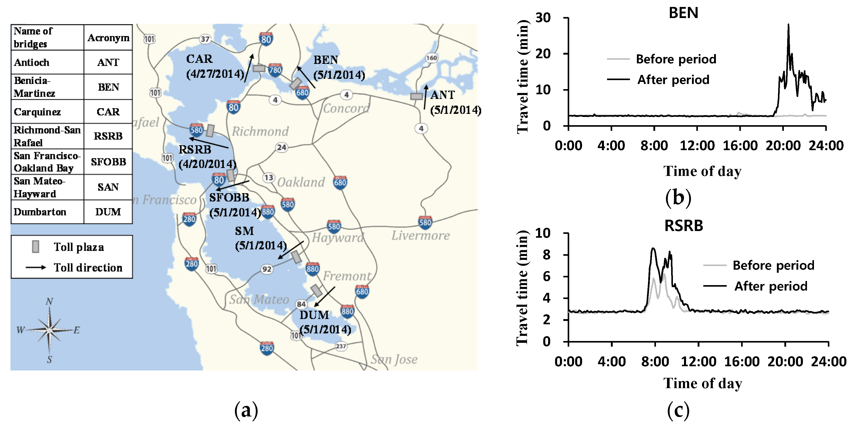
Figure 1a shows a map of the San Francisco Bay Area, and the small shaded boxes indicate the locations of toll plazas. The dates indicate when the changes in toll plaza staffing and the number of different types of lanes were made. The seven days following the staffing changes were excluded from the analysis to allow time for drivers to adjust to the new toll operation.
The Antioch (ANT) Bridge is comprised of three lanes, two of which operated as dedicated FasTrak lanes, while the remaining lane was a cash lane prior to 1 May 2014. One of the existing FasTrak lanes was converted to a cash lane during carpool operating hours (5:00 a.m. to 10:00 a.m. and 3:00 p.m. to 7:00 p.m.), but operated as a dedicated FasTrak lane at other times of the day. Staffing at the ANT was increased by four hours on weekdays—the cash lane requires a toll booth officer to be stationed at a booth, while FasTrak lanes do not. The travel times before and after the staffing/lane changes remain unaffected.
Benicia (BEN) Bridge comprises 17 lanes. Lanes 10–17 are “open road tolling” [14] lanes which use electronic collection to gather FasTrak information. Drivers can pass without the need to slow down, since there are no toll booths. Lanes 1–9 operate as cash lanes and FasTrak lanes at various times of the day. Cash lane operation hours at the BEN were reduced beginning 1 May 2014, resulting in significant delays (see Figure 1b) to the extent that staffing had to be readjusted two weeks later, as discussed in detail later in this paper.
Staffing at the Richmond San Rafael Bridge (RSRB) was increased to better accommodate cash lane demand. When the capacity for the FasTrak lanes is greater than the FasTrak demand, and the demand for the cash lane exceeds cash lane capacity, converting FasTrak lanes to cash lanes can reduce overall delay. Marked increase in travel times near the toll plazas were observed on two different days (see Figure 1c) following the increase in staffing. Although the factors that caused the marked increase in travel time remain elusive, this observation shed light on developing an analytical method. The data from the RSRB and the BEN were used to estimate the parameters of the proposed proxy measure [15].
No changes in staffing were made at the San Francisco Oakland Bay Bridge (SFOBB), and the changes in San Mateo (SM) and Dumbarton (DUM) bridges did not result in changes in travel times. Staffing at Carquinez (CAR) Bridge was reduced, but the travel time remained unaffected.

3. Challenges in Monitoring Traffic Conditions in Real-time Using Loop Detector Data

3.1. Monitoring Traffic Conditions

Monitoring the changes over extended segments of freeway is important in evaluating the effect of changes in capacity of toll plaza and travel times, and can be properly conducted if loop detectors span the entire segment [16,17]. However, if there is only one detector, attempting to monitor the changes in traffic conditions over extended segments solely based on localized data can result in erroneous conclusions and should be avoided in practice. This is illustrated in the following section.
Figure 2a,b shows the flow-occupancy relationship observed 2.5 miles upstream of the RSRB toll plaza. Only two out of seven investigated days displayed the relationship shown on Figure 2b, while, on the other days, the relationship remained within the free flow state, as shown in Figure 2a [15]. Investigation of the traffic data collected at the loop detector located 2.5 miles upstream of toll plaza can be used to monitor whether or not the tail of the queue reached the detector station. However, changes in traffic conditions over the 2.5-mile segment cannot be properly quantified based on the localized information from a loop detector or the toll booth discharge rate (i.e., observed flow departing the toll plaza); the toll booth will operate at its capacity while there is a queue at its upstream and downstream remains freely flowing [15]. This is further explained with the aid of Figure 2c,d.
Figure 2c,d show two hypothetical situations in which the queue began at the toll plaza ( TP ) and how their tail grew upstream. The traffic condition within the grey triangle is congested, while other sections of the time-space region remain freely flowing. In both figures, D indicates the location of loop detectors with respect to the tail of queue, while L is the length of the segment encompassing the entire queue that grew from the TP , and the travel times along this segment need to be compared to quantify the effect of the changes made at the TP .
Suppose that travel times were estimated solely based on the speed data reported from a loop detector location at D . When the tail of the queue does not reach D , the data collected at location D will exhibit the flow-occupancy relationship shown in Figure 2a. Utilizing the information from location D will assume that the traffic condition between D and the TP remains freely flowing, while the traffic travels at a reduced speed v i < V f within the congested region and underestimates travel times by t i (see Figure 2c).
When the tail of the queue reaches location D as shown in Figure 2d, the flow-occupancy relationship may display the pattern shown in Figure 2b. However, travel times still cannot be accurately estimated based on data collected at D . Figure 2d shows the trajectories of three vehicles that entered the congested region at times T a , T b and T c . When the first vehicle enters the congested region at time T a , the traffic condition at D is still freely flowing, and travel times estimated based on loop detector data from D at time T a can underestimate the travel time by t j . The estimated travel time of the second vehicle, which entered the congested region when the tail of the queue reached D at time T b , can be more accurately estimated. However, the estimated travel times of vehicles arriving after T b will be biased due to the unknown time spent in the queue upstream of D . The bias will be function of l , the length of queue upstream of D .
The magnitude of this bias can also be exacerbated depending on the speed of vehicles while they travel within the queue. The traffic state in the congested region can reside anywhere between S 1 and S 2 along the dotted straight line shown in Figure 2b. Based on the flow-occupancy relationship observed at D , the speed within the queue can range from V 2 to V 1 (see Figure 2e). The speed at each state can be estimated by calculating the slope of the straight line connecting the origin and each of the traffic states.
Figure 2f shows the relationship between the estimated travel times based on loop detector [18] located 2.5 miles upstream of the RSRB toll plaza and travel times reported by INRIX. As expected, the single sourced data do not adequately estimate the segment travel time. Therefore, using data from a single station is not appropriate in evaluating the effect of changes in toll plaza capacity and segment travel time.
With the advent of new GPS (global positioning system) devices, collecting segment travel times has become simple, and such information is readily available from a vendor such as INRIX [19]. However, monitoring changes in travel times alone will not provide the incremental capacity required at the toll plaza. Comparing the segment travel times and discharge rates also will not enable the agency to detect the onset of changes in traffic conditions leading to a marked increase in travel times: The travel time over an extended segment would not reveal the traffic becoming dense so long as the traffic remain freely flowing [17]. To this end, we developed a proxy measure to monitor changes in traffic conditions over extended freeway segments. This proxy measure can be used to determine the incremental capacity needed in response to changes in traffic conditions in real-time, as explained in the following section.

3.2. Locating the Back of the Queue Using Segment Travel Times

Figure 3a shows the travel time (i.e., average travel times across all lanes) reported by INRIX along the 2.87 miles of segment near the RSRB toll plaza observed on 15 May 2014. The length of the segment is greater than the longest tail of the queue originating from the toll plaza and encompasses links whose travel times were potentially affected by the changes made at the toll plaza. Figure 3b shows the cumulative travel time at time 7:10 a.m. on 15 May C   ( d , 07 : 10 ) with respect to the distance from the toll plaza. The horizontal distances between the white circles were predetermined by INRIX. The horizontal distances between links in the 5-mile segment are shown in Figure 3b. The y-axis represents the cumulative travel times from the TP . The slope of the curve represents the changes in time to travel the additional distance towards the toll plaza. The slope of C   ( d , 07 : 40 ) (see Figure 3c) is steep until it reaches 2.87 miles upstream of the TP , where it rapidly decreases. This indicates that the tail of the queue from the TP resided somewhere downstream of the segment, represented by the black circle labeled P , by 7:40 a.m. P divides the affected region from the unaffected region further upstream. Figure 3d,e shows the evolution of the location of P with respect to time, and this is how the length of the segment used in the analysis was determined.
After locating the tail of the queue, an input–output diagram [15] was constructed using the travel times. Since there are both on- and off-ramps within the segment, the arrival curve, constructed based on the travel times and the discharge rate the toll plaza, can be either greater or less than the actual arrival curve. However, as demonstrated below, the reconstructed input–output diagram using the traffic count and segment travel time provides sufficiently accurate information for the purpose of developing a proxy measure for dynamically determining toll staffing strategy.

4. Developing a Proxy Measure for Dynamically Determining Toll Plaza Capacity

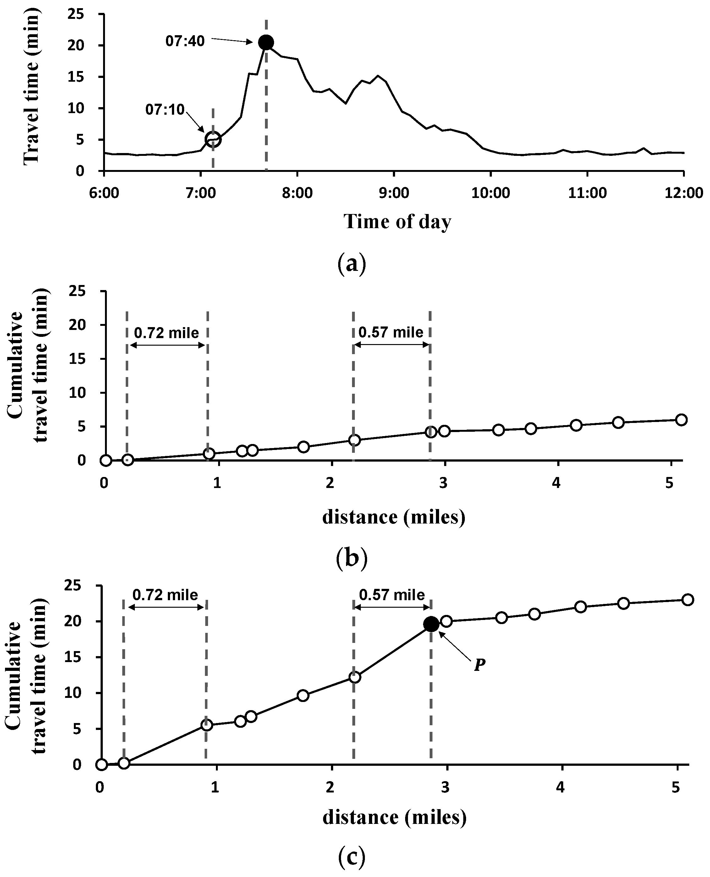
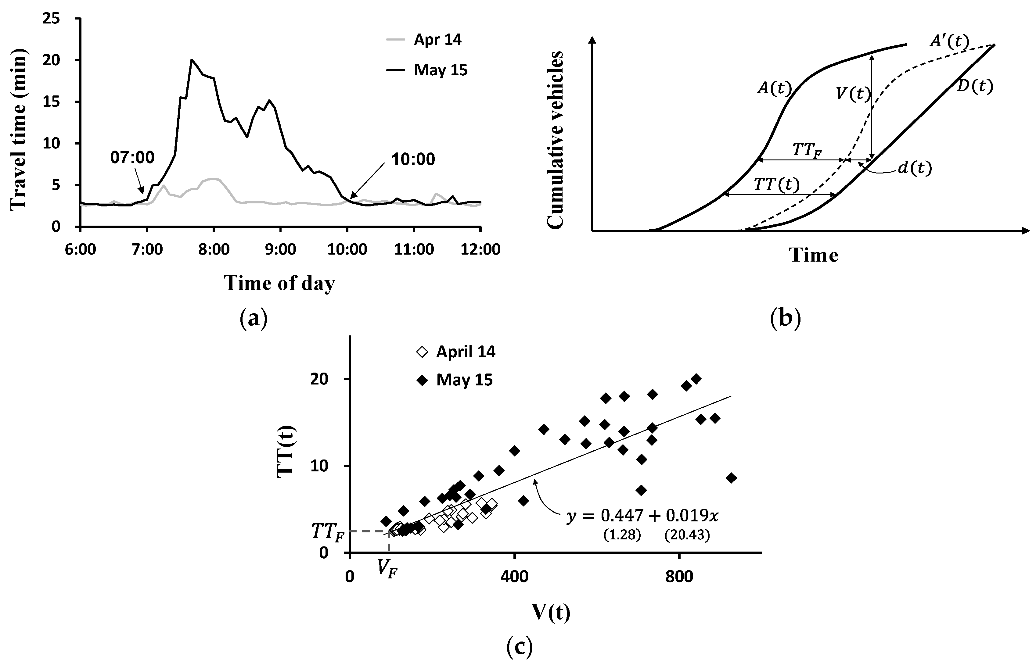
Figure 4a shows the segment travel times reported on 14 April and 15 May 2014, along the RSRB. Using the traffic count data and segment travel times, an input–output diagram can be constructed as shown in Figure 4b. The solid line labeled D ( t ) denotes the cumulative count of vehicles leaving the toll plaza with respect to time. Then, using the average travel times, D ( t ) was shifted back in time to reconstruct the cumulative arrival curve at the start of the segment, A ( t ) . V ( t ) , the vertical difference between A ( t ) and D ( t ) , is the estimated number of vehicles stored in the segment at time t (see Figure 4b and Equation (1)). When A ( t ) is shifted forward by the free flow travel, T T F (see A ( t ) in Figure 4b), the horizontal distance between A ( t ) and D ( t ) is the delay, d ( t ) . A ( t ) and D ( t ) will remain superimposed when traffic is freely flowing. The area under between A ( t ) and D ( t ) is the total delay.
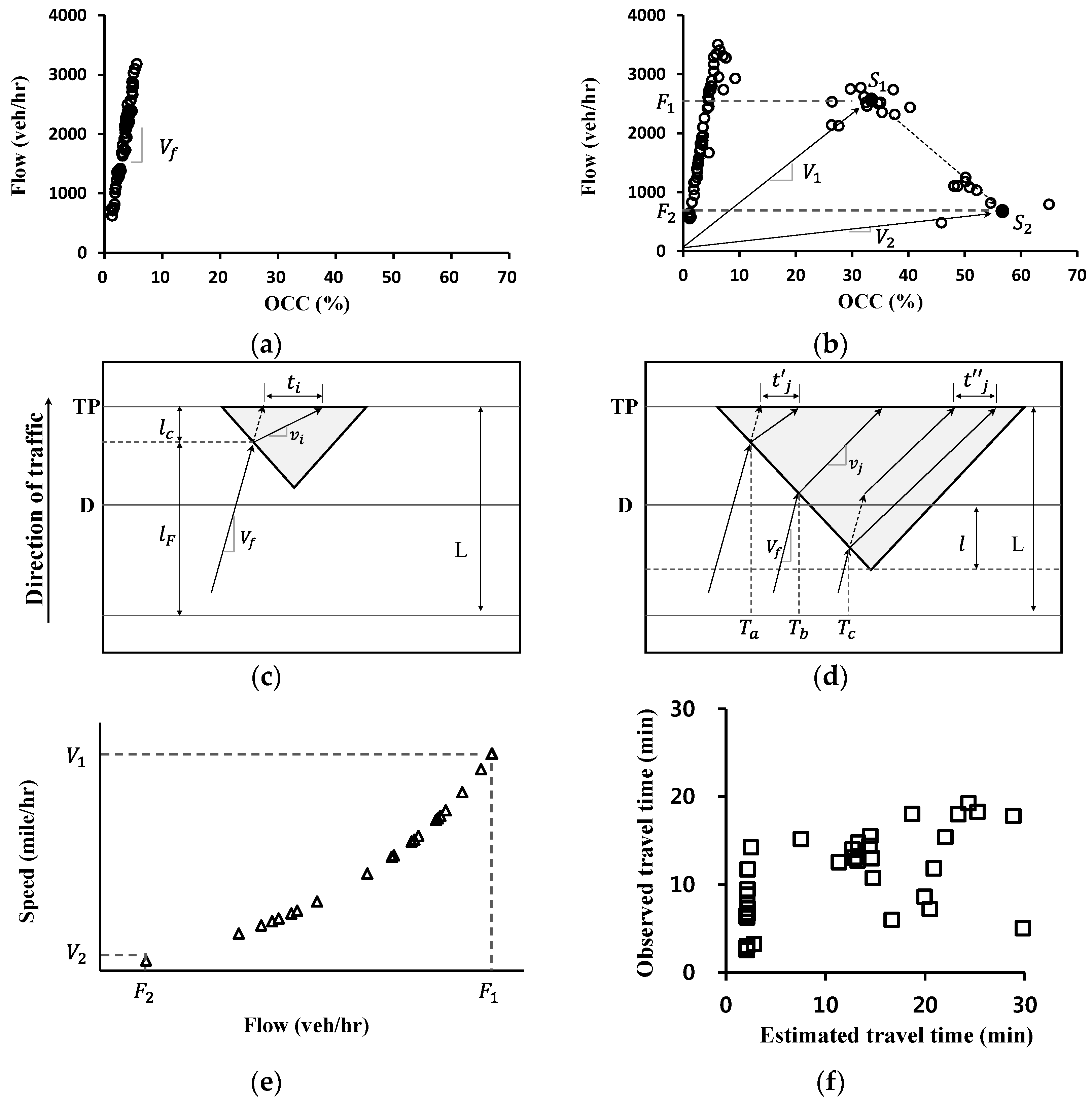
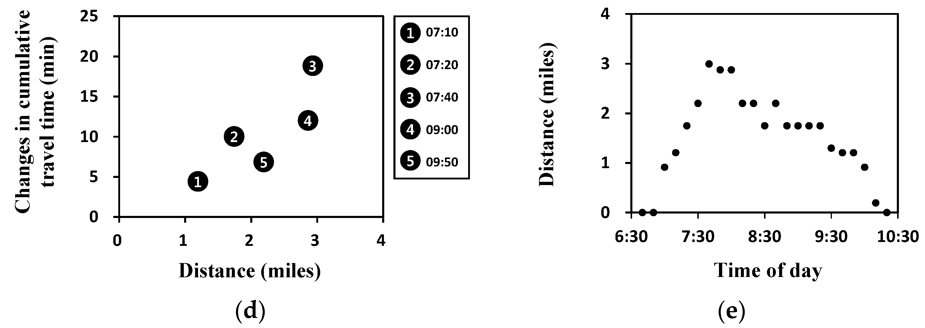
The changes in travel time that encompasses the queue near the upstream of the toll plaza were linearly approximated by the number of vehicles stored within the segment: An increase in queue length will change the portion of the trip that will be traveled by v f (see Figure 2c,d) under dense traffic conditions. Equation (2) is used based on this assumption, and V(t) is the proxy measure that was estimated following the procedure described in the preceding paragraph.
Equation (3) can be obtained by differentiating T T ( t ) , D ( t ) , and A ( t ) with respect to time. Note that the right side of equation consists of the difference between the rate of vehicles arriving at the cash lane, A ˙ C ( t ) , and the FasTrak lane, A ˙ F ( t ) and the corresponding cash lane, D ˙ C ( t ) , and FasTrak lane, D ˙ F ( t ) , discharge rates. Even though the combined demand for cash lanes and FasTrak lanes is less than the combined capacity, when the capacity for the two kinds of lanes is not properly assigned, the right side of equation can rapidly increase, resulting in a marked increase in travel times. This is what happened at the BEN Bridge after the staffing changes were made on 1 May 2014, as explained in detail later in this section.
Recall that V ( t ) is the only proxy measure developed to evaluate the relationship among T T ( t ) , A ˙ ( t ) , and D ˙ ( t ) . If the flow between upstream and downstream of the segment is conserved (i.e., no on- or off-ramps within the segment), V ( t ) shown in Equation (1) would be the number of vehicles stored in the segment. Although V ( t ) estimated in the manner described in the preceding paragraph can be biased depending on the locations of the ramps and the flow using them, it can still be used as a proxy measure as shown in Figure 4c.
A ( t ) D ( t ) = V ( t )
T T ( t ) = α + β V ( t )
T T ˙ ( t ) = β [ A ˙ ( t ) D ˙ ( t ) ]
T T ˙ ( t ) = β [ ( A ˙ C ( t ) D ˙ C ( t ) ) + ( A ˙ F ( t ) D ˙ F ( t ) ) ]
The estimated V ( t ) from 14 April and 15 May 2014, are used to evaluate their relationship with T T ( t ) (see Figure 4c). Compared with Figure 2f, V ( t ) displays a strong linear relationship with T T ( t ) . T T F shown on the y-axis of Figure 4c is the freely flowing travel time and V F is the vehicle accumulation within the segment that can maintain the free flowing speed. When V ( t ) exceeds V F , the T T ( t ) begins to linearly increase. The slope of the line essentially indicates the changes in T T ( t ) resulting from the difference in A ˙ ( t ) and D ˙ ( t ) (see Equation (3)).
The operator needs to carefully determine the number of cash and FasTrak lanes, since V ( t ) can increase (see Equation (4)) whenever the demand for FasTrak or cash lanes exceed the capacity of FasTrak or cash lanes. As noted earlier, toll staffing at the RSRB was increased on 1 May to better accommodate the cash lane demand, and a marked increase in travel time was observed on two of the seventeen days evaluated following the changes. This increase in travel time was greater than the typical delay observed prior to the changes and was accompanied by an increase in V ( t ) . The increase in V ( t ) could have been the result of an increase in FasTrak demand each day coupled with a decrease in FasTrak capacity, as some of the FasTrak capacity was allocated to the cash lane capacity. However, this could not be confirmed with the data available from the RSRB. If this marked increase in travel times (at the RSRB) observed in two days were, indeed, a result of having fewer number of FasTrak lanes, the operator could evaluate the impact of converting existing cash lanes to FasTrak lanes using Equation (4). Discharge rate reported from the toll plazas (see Figure 1a) indicated that a FasTrak lane can serve about 1200–1300 vehicles per hour (vph) and a cash lane can serve about 360 vph while the toll plaza remains an active bottleneck [15,16,17]: The presence of a queue upstream of the toll plaza and downstream remaining freely flowing were visually confirmed by the toll plaza officers in estimating the FasTrak and cash lane capacity. The operator can increase the combined FasTrak lane capacity by an increment of 1200–1300 vph while decreasing the combined cash lane capacity by 360 vph in Equation (4) to estimate V ( t ) and the resulting T T ( t ) (see Figure 4c). Since V ( t ) is a proxy measure, and toll plaza capacity for cash and FasTrak changes in discrete increments, accurately estimating FasTrak and cash lane capacity is not a requirement for using proposed method.
Suppose the changes in T T ( t ) and Δ T T ( t ) were observed over some time T d (see Equation (5)), and the relationship between V ( t ) and T T ( t ) shown in the figure holds. V ( t ) would have been changed by Δ V ( t ) over T d . When T d is set to one hour, then Δ T T is the increase in travel time expected to accompany the difference in A ˙ ( t ) and D ˙ ( t ) that is sustained for an hour. Dividing observed T T ( t ) by β would provide an estimate of the additional capacity that needs to be maintained to change Δ T T ( t ) to 0 based on the proposed model (see Equation (6)).
Δ T T = β · Δ V = β [ A ˙ ( t ) D ˙ ( t ) ] · T d
Δ T T β · T d = [ A ˙ ( t ) D ˙ ( t ) ]
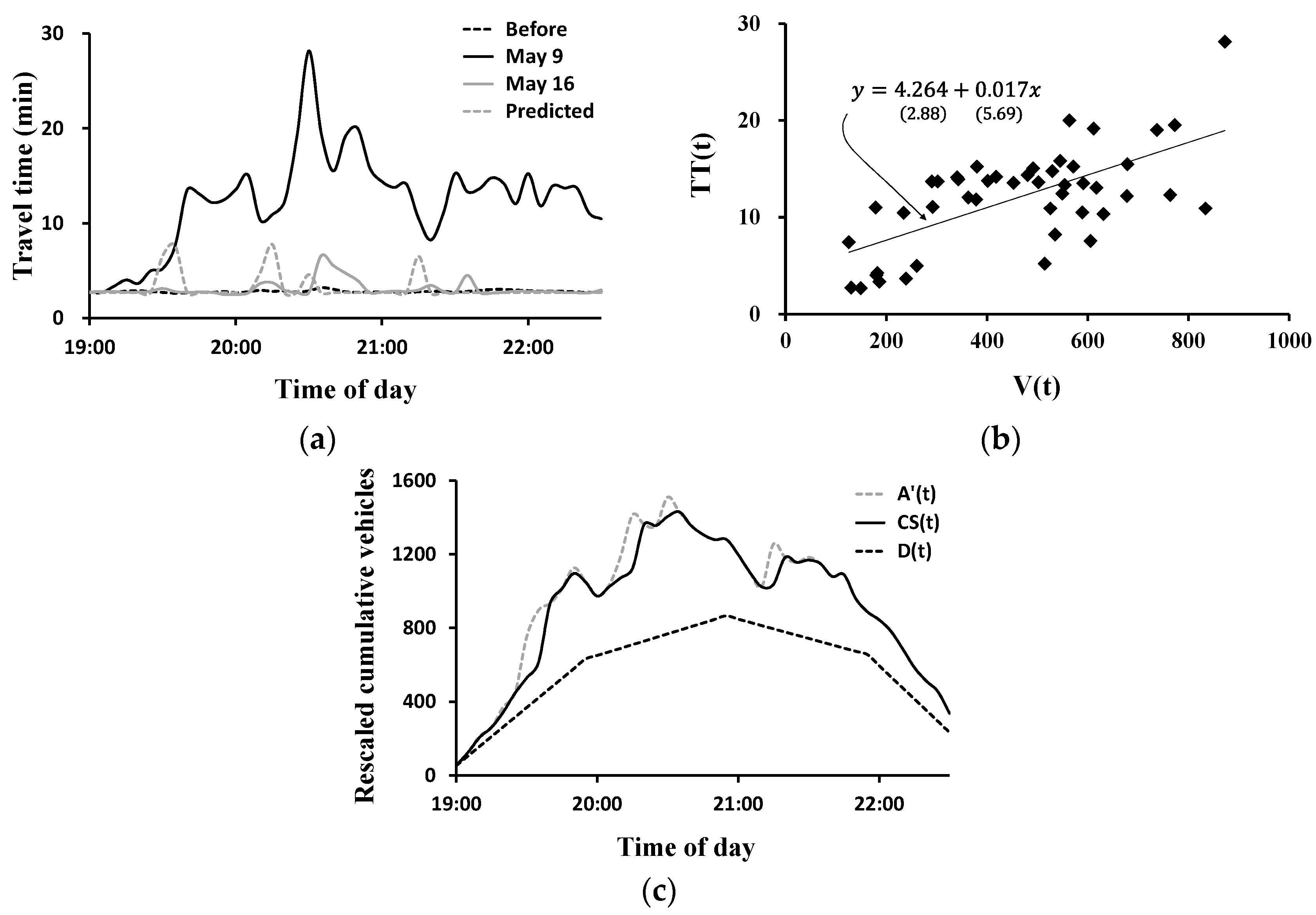
Travel times along a 2.97-mile segment leading to the BEN during the Friday evening peak period are shown in Figure 5a. The dotted black line represents the average Friday afternoon travel times observed during the before period. The solid black line represents the travel time observed on 9 May 2014. Recall that the facility has seventeen lanes, among which lanes 10–17 are open road tolling lanes, while a varying number of lanes among lanes 1–10 operated as cash lanes throughout the day. Staffing for the cash lanes was reduced from five lanes to three lanes for the Friday evening peak operation beginning on 1 May 2014: While D ˙ C ( t ) has been reduced, the number of open road tolling lanes remains the same—[ A ˙ F ( t ) D ˙ F ( t ) ] can be assumed to have remained constant. A marked increase in travel times accompanied the change in staffing and lane availability (see the travel on 9 May in Figure 5a), and complaints were filed by commuters. After an in-depth discussion among toll plaza stakeholders, it was agreed that the staffing of cash lanes at the BEN for the Friday evening period would be increased from three lanes to four lanes. The revised scheduled was implemented on 16 May 2014, and travel times on 16 May returned to a level similar to the initial condition. Figure 5b shows the relationship between V ( t ) and T T ( t ) observed at the BEN on 9 May 2014.
Based on the observed relationship between V ( t ) and T T ( t ) , and assuming that the demand on 16 May would be comparable to that of 9 May, the proposed model can be used to predict segment travel times in a scenario of an increased number of cash lanes. The cash lane capacity of the toll plaza is roughly estimated to be 360 vehicles per hour based on observations at the toll plaza. Since drivers using the cash lane can pay either with cash or via the electronic transponder, as was stated in the introduction, this observed cash lane capacity would have been affected by electronic transponder users. Assuming A ˙ ( t ) would remain comparable to the previous Friday, the solid black line in Figure 5c is the estimated rescaled cumulative vehicle count passing the toll plaza under the increased capacity schedule, C S ( t ) . D ( t ) (represented by the dotted black line in Figure 5c) depicts the rescaled departure curve at the toll plaza if staffing had not been increased.
In the figure, A ( t ) is the rescaled A ( t ) shifted forward in travel time. Notice how the vertical separation between A ( t ) and C S ( t ) disappears the majority of the time, indicating that the traffic will remain mostly freely flowing in response to opening up an additional cash lane. The proposed model would predict delays where A ( t ) and C S ( t ) do not remain superimposed. The vertical separation is the excess vehicle accumulation based on the proxy measure. By adding this number to V F (see Figure 4c) and using the relationship shown in Equation (2), the travel times during the Friday afternoon peak after the staffing increase were predicted—the parameters for Equation (2) were calibrated and are shown in Figure 5b. The predicted travel times are shown together with the observed travel times (see the light grey line labeled “May 16” and dotted grey line labeled “Predicted”). The predicted and observed travel times were remarkably comparable.
The proposed model can be used to evaluate the impact of sudden increase in A(t) on TT(t) using the observed V(t) and TT(t) relation near the toll plaza. Thus, the agency can consider an increase in toll plaza capacity when the projected travel time is expected to exceed the threshold value that the agency predetermined based on value of time [20] and operating cost. Since frequently adjusting toll plaza capacity can create confusion among the drivers, the agency should consider requiring minimum time lapse before adjusting toll plaza capacity and also set the range of capacity that can be dynamically changed.

5. Concluding Remarks

When the demand for FasTrak and cash lanes is not properly balanced, increases in travel times can result, even if the combined number of FasTrak and cash lanes exceed the combined FasTrak and cash lane demand. As was illustrated in preceding section, changing the staffing of the toll plazas in the San Francisco Bay Area without carefully considering the demand for FasTrak and cash lanes resulted in increasing delays at two locations. Particularly at the RSRB, although the factors that contributed to such an increase in travel time remain elusive, the observed segment travel times and discharge rate at the RSRB shed light on developing a proxy measure that can be used to determine the toll plaza capacity and segment travel times. The data from the RSRB and Ben was applied to develop a proposed model as a proxy measure and validate the model.
The proposed method can aid government agencies in dynamically adjusting toll plaza capacity in response to sudden shifts in demand due to various situations of failure and in evaluating the effect of toll plaza capacity without requiring traffic data from loop detectors at strategic locations over extended freeway segments.
The observed relationship between V ( t ) and T T ( t ) near toll plaza was linear such that its parameters were estimated using linear regression. If the observed relation had not followed simple linear relationship because of accidents [21] or on- and off-ramps within the segment, the proxy measure needs to employ the non-linear relationship between V(t) and TT(t) in dynamically determining the toll booth capacity. The reproducibility of linear relationship between V(t) and TT(t) from a longer freeway segment that encompasses on- and off-ramps are the subject of future study. This paper only considered the effect of changing toll plaza capacity and did not quantify the effect of changing arrival rate after controlling arrival rate using dynamic traffic control strategies, such as system wide ramp metering or variable change signage. Additionally, this paper did not consider other factors such as lane selection [22]. These are subjects of future study. Nevertheless, this paper can aid the adjustment for the dynamic change in capacity as an effectual proxy measure, even with these limitations.

Acknowledgments

Findings and views reported in this paper are solely the opinions of the authors and do not represent the view of the California Department of Transportation. The authors greatly appreciate David Seriani, Rodney Oto, and Chris Tseng for providing support for this study. Special thanks to Carl Crosby and Russell Sweden from Caltrans Maintenance Toll Bridge Operations for providing invaluable comments and data. This work was partly supported by the Institute of Construction and Environmental Engineering of Seoul National University, Jungseok Logistics Foundation Grant, and National Research Foundation of Korea (2010-0029446 and 2015R1C1A1A02037285).

Author Contributions

The empirical data are analyzed by Choelsun Kim and Dong-Kyu Kim. Koohong Chung provided data and constructed the model. Choelsun Kim and Koohong Chung prepared the manuscript. Seung-Young Kho and Seungmo Kang contributed to the paper by suggesting the overall framework and the research idea, revising the manuscript, and providing overall supervision of this work.

Conflicts of Interest

The authors declare no conflict of interest.

Notations

The following notations are used in this manuscript:
A ( t ) =cumulative arrival count of vehicles at toll plaza;
A ˙ ( t ) =differenciated A ( t ) ;
A ˙ C ( t ) =corresponding cash lane, A ˙ ( t ) ;
A ˙ F ( t ) =corresponding FasTrak lane, A ˙ ( t ) ;
D ( t ) =cumulative count of vehicles leaving the toll plaza;
D ˙ ( t ) =differenciated D ( t ) ;
D ˙ C ( t ) =corresponding cash lane, D ˙ ( t ) ;
D ˙ F ( t ) =corresponding FasTrak lane, D ˙ ( t ) ;
T T ( t ) =travel time of the segment;
T T ˙ ( t ) =differenciated T T ( t ) ;
Δ T T =quantity of changes in T T ( t ) ;
T d =observed time set to an hour;
V ( t ) =estimated number of vehicles stored in the segment;
Δ V =quantity of changes in V ( t ) .

References

  1. Edie, L.C. Traffic delays at toll booths. Oper. Res. 1954, 2, 107–138. [Google Scholar] [CrossRef]
  2. Burris, M.W.; Hildebrand, E.D. Using microsimulation to quantify the impact of electronic toll collection. ITE J. 1996, 66, 21–24. [Google Scholar]
  3. Astarita, V.; Florian, M.; Musolino, G. A microscopic traffic simulation model for the evaluation of toll station systems. In Proceedings of the IEEE 2001 Intelligent Transportation Systems, Oakland, CA, USA, 25–29 August 2001.
  4. Al-Deek, H.M.; Mohammed, A.A. Simulation and Evaluation of the Orlando-Orange County Expressway Authority (OOCEA) Electronic Toll Collection Plazas Using TPSIM; BC 096–11; Florida Department of Transportation: Orlando, FL, USA, 2000. [Google Scholar]
  5. Al-Deek, H.M.; Mohamed, A.A.; Radwan, E.A. A new model for the evaluation of traffic operations at electronic toll collection plazas. Transp. Res. Rec. 2000, 1710, 1–10. [Google Scholar] [CrossRef]
  6. Al-Deek, H.M.; Mohamed, A.A.; Malone, L. A new stochastic discrete-event micro simulation model for evaluating traffic operations at electronic toll collection plazas. Intell. Transp. Syst. 2005, 9, 205–219. [Google Scholar] [CrossRef]
  7. Correa, E.; Metzner, C.; Nino, N. TollSim: Simulation and evaluation of toll stations. Int. Trans. Oper. Res. 2004, 11, 121–138. [Google Scholar] [CrossRef]
  8. Ceballos, G.; Curtis, O. Queue Analysis at Toll and Parking Exit Plazas: A Comparison Between Multi-Server Queuing Model and Traffic Simulation. In Proceedings of the ITE 2004 Annual Meeting and Exhibit, Lake Buena Vista, FL, USA, 1–4 August 2004.
  9. Chien, S.I.; Spasovic, L.N.; Opie, E.K.; Korikanthimathi, V.; Besenski, D. Simulation-based Analysis for Toll Plazas with Multiple Toll Methods. In Proceedings of the 84th Annual Meeting of the Transportation Research Board, Washington, DC, USA, 9–13 January 2005.
  10. Ozbay, K.; Mudigonda, S.; Bartin, B. Microscopic Simulation and Calibration of An Integrated Freeway and Toll Plaza Model. In Proceedings of the 85th Annual Meeting of the Transportation Research Board, Washington, DC, USA, 22–26 January 2006.
  11. Zarrillo, M.; Radwan, E.A. Methodology SHAKER and the capacity analysis of five toll plazas. J. Transp. Eng. 2009, 135, 83–93. [Google Scholar] [CrossRef]
  12. Russo, C.; Harb, R.; Radwan, E.A. Calibration and verification of SHAKER, a deterministic toll plaza simulation model. J. Transp. Eng. 2009, 136, 85–92. [Google Scholar] [CrossRef]
  13. Wander, M.; Peirce, J.J. Formulation, structure, and analysis of a model to optimize staffing levels at border checkpoints. J. Transp. Eng. 2011, 137, 789–795. [Google Scholar] [CrossRef]
  14. Deakin, E.; Frick, K.T.; Cervero, R.; Skabardonis, A.; Barnes, I.; Kingsley, K.; Rubin, J.; Murakami, J.; Amaro, J.; Jensen, E. Bay Bridge Toll Evaluation: Final Report; Global Metropolitan Studies and the University of California: Berkeley, CA, USA, 2011. [Google Scholar]
  15. Daganzo, C.; Daganzo, C.F. Fundamentals of Transportation and Traffic Operations; Pergamon Press: Oxford, UK, 1997. [Google Scholar]
  16. Coifman, B. Estimating travel times and vehicle trajectories on freeways using dual loop detectors. Transp. Res. Part A: Pol. Pract. 2002, 36, 351–364. [Google Scholar] [CrossRef]
  17. Chung, K.; Rudjanakanoknad, J.; Cassidy, M.J. Relations between traffic density and capacity drop at three freeway bottlenecks. Transp. Res. Part B: Methodol. 2007, 41, 82–95. [Google Scholar] [CrossRef]
  18. PeMS. Available online: http://pems.dot.ca.gov (accessed on 25 July 2014).
  19. INRIX. Available online: http://www.inrix.com/inrixtraffic.asp (accessed on 25 July 2014).
  20. Mackie, P.J.; Jara-Dıaz, S.; Fowkes, A.S. The value of travel time savings in evaluation. Transp. Res. Part E: Logist. Transp. Rev. 2001, 37, 91–106. [Google Scholar] [CrossRef]
  21. Li, Z.; Chung, K.; Cassidy, M.J. Collisions in freeway traffic: The influence of downstream queues and interim means to address it. Transp. Res. Rec. 2013, 2396, 1–9. [Google Scholar] [CrossRef]
  22. Dubedi, A.; Chakroborty, P.; Kundu, D.; Reddy, K. Modeling automobile drivers′ toll-lane choice behavior at a toll plaza. J. Transp. Eng. 2012, 138, 1350–1357. [Google Scholar] [CrossRef]
Figure 1. (a) Toll plazas in the San Francisco Bay Area. (b) and (c) Average travel times near bridges during weekdays before and after changes in toll plaza staffing.
Applsci 06 00087 g001
Figure 2. (a) Fundamental diagram remained within the free flow state. (b) Fundamental diagram entering the unstable flow state, monitoring the tail of the queue and determining affected links. (c) Hypothetical situation in which the queue started from the toll plaza but not reaching D. (d) Hypothetical situation in which the queue started from the toll plaza and reaching D. (e) Estimated speed within the queue. (f) Relationship between estimated travel times and observed travel times.
Applsci 06 00087 g002
Figure 3. (a) Travel time along the 2.87-mile segment near the RSRB (Richmond San Rafael Bridge) toll plaza observed on 15 May. (b) Snapshot of cumulative travel time at time 07:10. (c) Snapshot of cumulative travel time at time 07:40. (d) Changes in cumulative travel time from P to the toll booth. (e) Length of the queue.
Applsci 06 00087 g003aApplsci 06 00087 g003b
Figure 4. (a) Segment travel times reported by INRIX. (b) Input–output diagram using the traffic count data from the toll plaza and segment travel times. (c) Relationship between cumulative count of vehicles and segment travel times from before and after period (the numbers in parentheses are t-value of parameters).
Applsci 06 00087 g004
Figure 5. (a) Changes in travel times near the BEN (Benicia) Bridge toll plaza during Friday afternoon commute period. (b) Relationship between cumulative count of vehicles and segment travel times observed on 9 May 2014 (the numbers in parentheses are t-value of parameters). (c) Rescaled cumulative departure curve.
Applsci 06 00087 g005

