Detecting the Presence of High Water-to-Cement Ratio in Concrete Surfaces Using Highly Nonlinear Solitary Waves

Abstract

We describe a nondestructive evaluation (NDE) method based on the propagation of highly nonlinear solitary waves (HNSWs) to determine the excess of water on the surface of existing concrete structures. HNSWs are induced in a one-dimensional granular chain placed in contact with the concrete to be tested. The chain is part of a built-in transducer designed and assembled to exploit the dynamic interaction between the particles and the concrete. The hypothesis is that the interaction depends on the stiffness of the concrete and influences the time-of-flight of the solitary pulse reflected at the transducer/concrete interface. Two sets of experiments were conducted. In the first set, eighteen concrete cylinders with different water-to-cement (w/c) ratios were cast and tested in order to obtain baseline data to link the ratio to the time of flight. Then, sixteen short beams with fixed w/c ratio, but subject to water in excess at one surface, were cast. The novel NDE method was applied along with the conventional ultrasonic pulse velocity technique in order to determine advantages and limitations of the proposed approach. The results show that the time of flight detected the excess of water in the beams. In the future, the proposed method may be employed in the field to evaluate rapidly and reliably the condition of existing concrete structures and, in particular, concrete decks.

1. Introduction

In concrete and cement based structures, the early stage of hydration and the conditions at which curing occurs, influence the quality and the durability of the final products. For instance, as a result of the chemical reactions between water and the cement during hydration, the mixture progressively develops mechanical properties. Final set for the mixture is defined as the time that the fresh concrete transforms from plastic into a rigid state. At final set, measurable mechanical properties start to develop in concrete and continue to grow progressively. The durability and the strength of concrete may deviate from design conditions as a result of accidental factors. Some of these factors are water-to-cement (w/c) ratio not controlled well and rainfall that permeates the fresh concrete or dampens the forms prior to casting. As such, the development of nondestructive evaluation (NDE) methods able to determine anomalous concrete conditions is very much needed, and has been a long-standing challenge in the area of material characterization. To date, many NDE methods for concrete exist, and some of them resulted in commercial products. The interested reader is referred to the excellent monograph [1] to gain a holistic knowledge of such methods. The most common technique is probably the one based on the propagation of bulk ultrasonic waves through concrete. This approach measures the speed of the waves propagating through the thickness of the test object to determine the elastic modulus using an empirical formula [1,2,3,4,5,6,7,8,9,10]. This approach is usually referred to as the ultrasonic pulse velocity (UPV) method. If the access to the back wall of the sample is impractical, the ultrasonic testing is conducted in the pulse-echo mode. A popular commercial system is the Schmidt hammer [11,12,13,14], which consists of a spring-driven steel hammer that hits the specimen with a defined energy. Part of the impact energy is transmitted to the specimen and absorbed by the plastic deformation of the specimen and the remaining impact energy is rebounded. The rebound distance depends on the hardness of the specimen and the condition of the surface. The harder the surface, the shorter the penetration time (or depth) and therefore the higher is the rebound.

Despite decades of research and developments, much research is still ongoing [13,15,16,17,18,19,20,21,22,23,24,25,26,27,28] and many interesting works covering a wide spectrum of NDE techniques are being investigated. In this paper, we propose an NDE method based on the propagation of highly nonlinear solitary waves (HNSWs) along a 1D chain of spherical particles placed in contact with the concrete to be tested. These waves are compact mechanical waves that can form and travel in highly nonlinear systems, such as a chain of elastically interacting spheres. The interaction between two adjacent beads is governed by the Hertz’s law [29,30] F = Aδ^3/2, where F is the compression force between the granules and δ is the closest approach of their centers. The coefficient A is equal to E·d^1/2/[3·(1 − ν²)] where E, d, and ν are the modulus of elasticity, diameter, and Poisson’s ratio of the spheres, respectively.

The most common way to induce a solitary pulse, hereinafter indicated as the incident solitary wave (ISW), is by tapping the first particle of the chain with a particle striker having at least the same mass of the individual beads forming the chain. Some researchers have demonstrated that a piezo-actuator [31,32] or even laser pulses [33] can be used as well. When the ISW reaches the interface with the material to be tested, the pulse is partially reflected giving rise to the primary reflected solitary wave (PSW). Both ISW and PSW can be sensed either by a force sensor located at the opposite end of the chain or by embedding a sensor bead along the chain. For a detailed description of the underlying basis of HNSWs, see ref. [34,35,36,37].

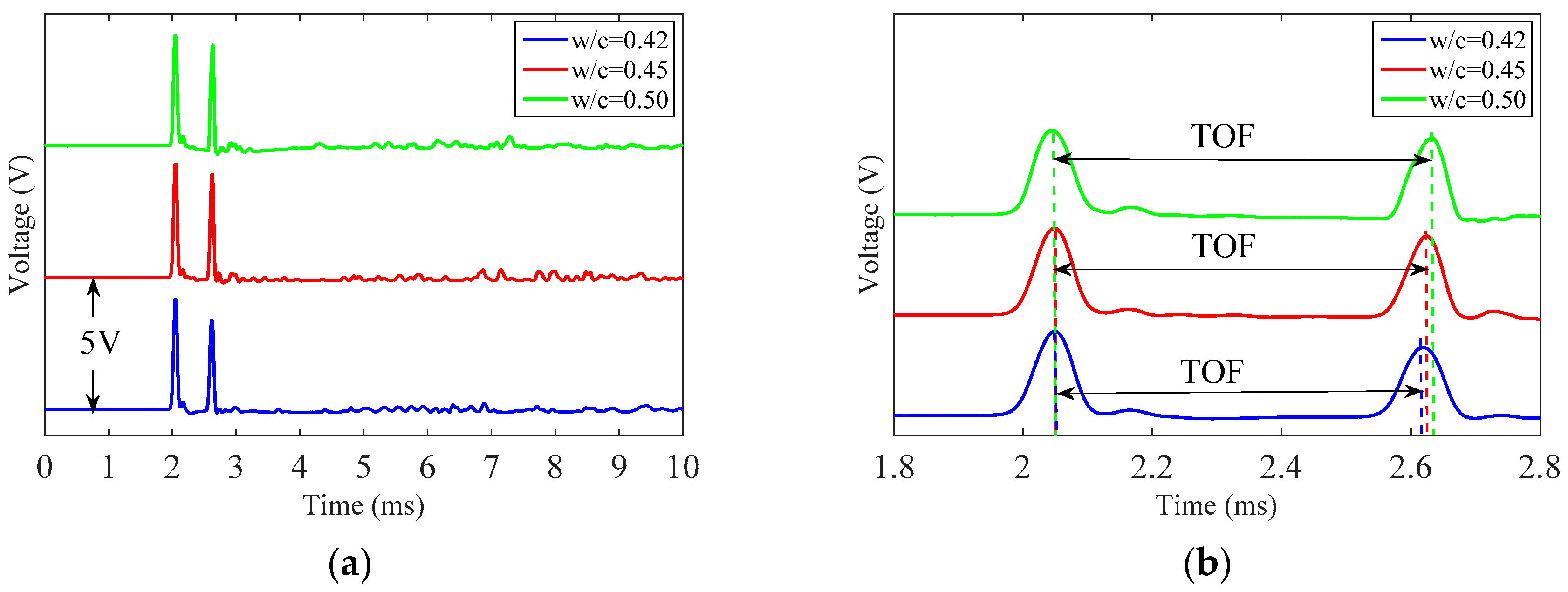
The study presented here expands on a recent work where HNSWs were used to determine the elastic modulus of concrete cylinders fabricated with three different w/c ratios, namely 0.42, 0.45, and 0.50 [38]. In the present work, we use some of the findings from [38] to predict water in excess in short concrete beams made with w/c = 0.42 but corrupted with water. Two conditions were simulated. The first one consisted of standing water in formworks prior to pouring concrete, whereas the second condition consisted of sprinkling water above the fresh concrete during casting and surface finishing. These two conditions may reflect adverse weather in the field. The objective of the study was the development of a system that, unlike the UPV method, can predict localized deterioration conditions associated with poor quality w/c ratios.

Three HNSW transducers, referred with the descriptor P1, P2, and P3, were used to quantify the elastic modulus of the beams. Owing to the novelty of the transducers design it was decided to assemble and test three of them in order to demonstrate and quantify the repeatability of the design and to quantify any variation of the results associated with differences in the assembly. The findings were then compared to the results of a conventional UPV test in order to evaluate and prove advantages and eventually limitations of the proposed approach.

With respect to ultrasonic-based NDE, the HNSW-based approach: (1) exploits the propagation of HNSWs confined within the particles of the chain; (2) employs a cost-effective transducer; (3) does not require any knowledge of the sample thickness; (4) does not need access to the back-wall of the sample; (5) provides point-like information rather than information about the average characteristics of the whole sample. The method also differs significantly from the Schmidt hammer. In fact, the hammer can be used to test hardened material but the HNSW approach can also characterize fresh concrete and cement as demonstrated in [39,40]; only one parameter, the rebound value, is used in the Schmidt hammer test, while multiple HNSW features can, in principle, be exploited to assess the condition of the underlying material. The hammer may induce plastic deformation or microcracks into the specimen, while the HNSW approach is purely nondestructive.

The paper is organized as follows. The next section describes the concrete samples, the design of the HNSW transducers, and the test protocols adopted throughout the study. Section 3 presents the experimental results associated with the concrete cylinders and it is largely excerpted from reference [38] in order to provide a comprehensive knowledge in support of the findings of Section 4 that presents the results associated with the short beam. The latter represents the core novelty of the present paper. Finally, Section 5 summarizes the findings of the project and provides some suggestions for future studies.

2. Experimental Setup

2.1. Materials

To set the baseline data, eighteen concrete cylinders were cast and tested: nine were evaluated nondestructively, whereas the remaining nine were tested according to the ASTM C469. The cylinders were 152.4 mm (6 in.) in diameter and 304.8 mm (12 in.) high. Three w/c ratios, namely 0.42, 0.45, and 0.50, were considered.

The materials are listed in

Table 1a. Material used in the concrete mixtures.

Material	Specific Gravity	Water Absorption Capacity (%)
Cement	3.15	n/a
Coarse aggregate	2.71	0.50
Fine aggregate	2.67	1.24
GGBFS 1	2.83	n/a

¹ ground-granulated blast-furnace slag.

and the mixture designs are presented in

Table 1b. Ingredients of each concrete batch.

Batch	1	2	3
w/c ratio	0.42	0.45	0.50
Paste vol./concrete vol.	0.30	0.30	0.30
Air content (%)	6.50	5.00	6.25
Coarse agg. (kg/m3)	1054	1054	1054
Fine agg. (kg/m3)	666	666	666
Cement (kg/m3)	303	291	274
GGBFS (kg/m3)	101	97	91
Water (kg/m3)	170	175	183
Slump (mm)	133	95	203

. To ease identification, we labeled the samples according to

Table 1c. Detailed information about the concrete cylinders. The samples evaluated with the HNSW (highly nonlinear solitary wave)-transducers were wet and tested after 28 days of curing. The samples evaluated with the UPV (ultrasonic pulse velocity) were wet and tested after 29 days of curing. The samples subjected to compressive load were tested saturated after 28 days of curing.

w/c Ratio	Number of Cylinders	NDE Sample Labels	ASTM C469 Sample Labels
0.42	6	42A, 42B, 42C	42D, 42E, 42F
0.45	6	45A, 45B, 45C	45D, 45E, 45F
0.50	6	50A, 50B, 50C	50D, 50E, 50F

.

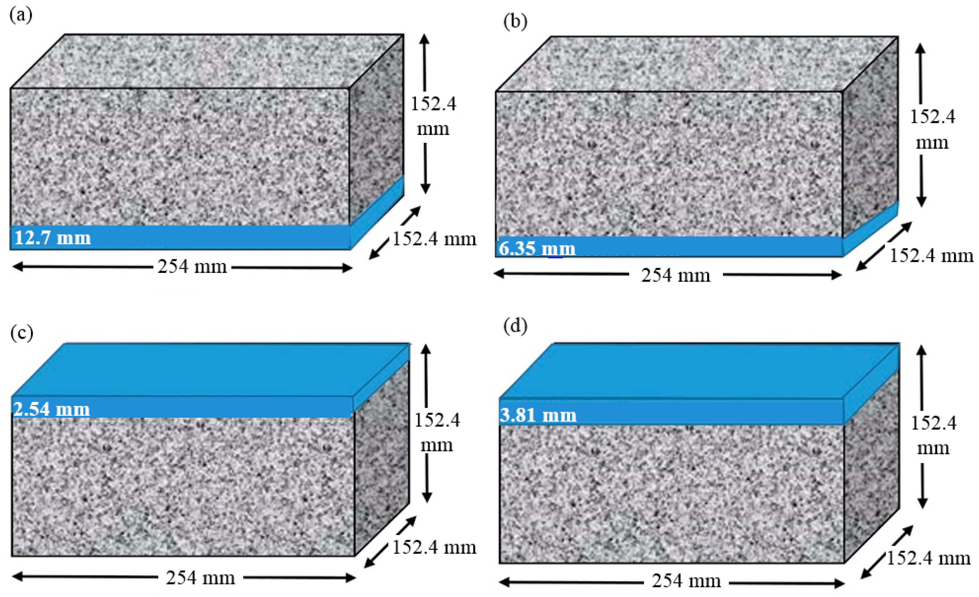
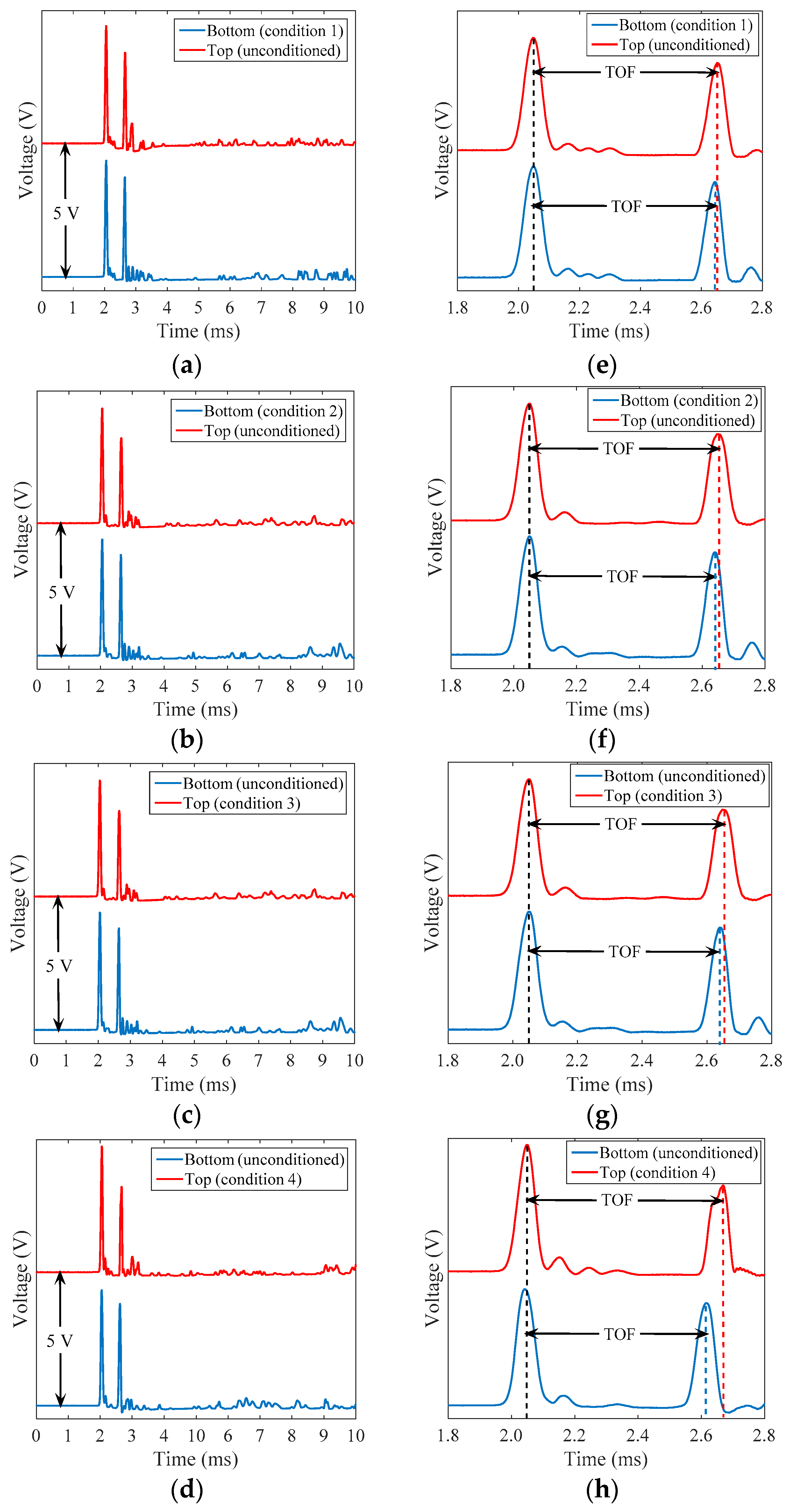
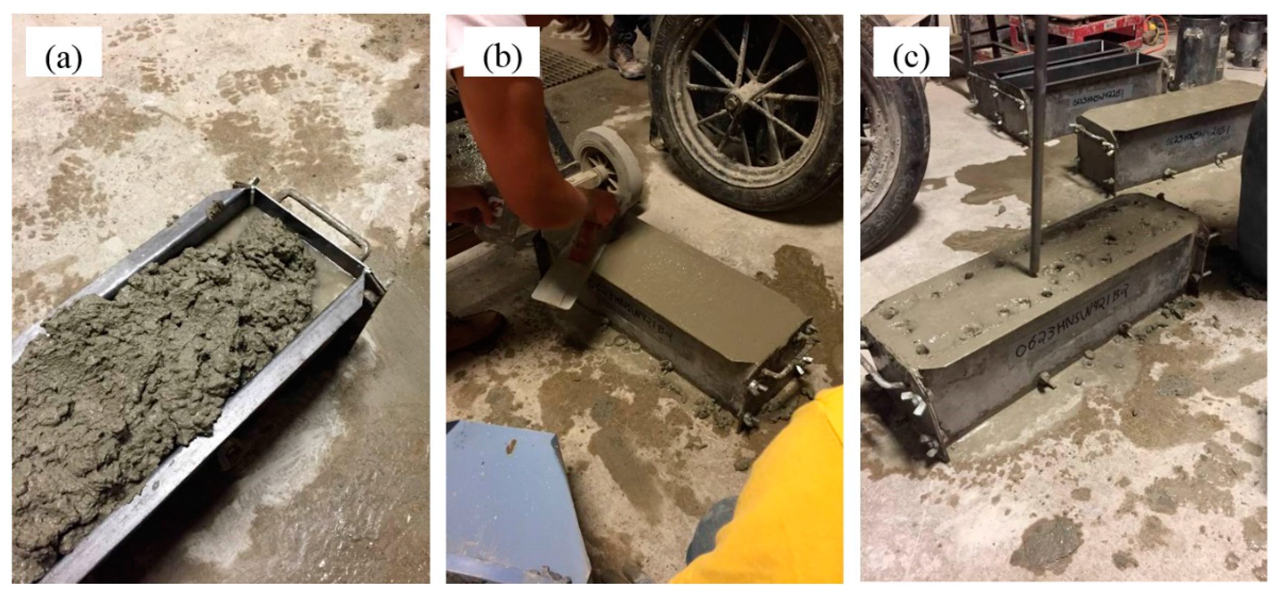
Then, sixteen 15.2 cm × 15.2 cm × 30.4 cm (6 in. × 6 in. × 12 in.) beams were fabricated using concrete mix design with w/c = 0.42. The beams were subject to the four different scenarios sketched in Figure 1. Each scenario represented either two surface finishing or two standing water situations in the formworks. Conditions 1 and 2 reflected the field case where water accumulates on the formwork as a result of rainfall prior to the placement of the concrete. To create Conditions 1 and 2, a predetermined volume of water based on the surface area of the beam mold was measured and poured on the sealed molds. Concrete was placed as evenly as possible into the molds and a shaft vibrator was then used to consolidate the concrete mixture before finishing the top surface. During the fabrication, the standing water was seen migrating to the top as shown in Figure 2a. After consolidation, the top surfaces of the beam molds were finished.

Conditions 3 and 4 simulated instead the occurrence of rainfall during placement and finishing of the concrete. To create these conditions, a specific procedure was developed in an effort to best simulate the finishing of rainfall that would occur on a job site. The procedure began by placing the concrete into the dry beam mold without any consolidation or finishing performed. The predetermined volume of surface water, similarly based on the base area of the mold, was then divided into thirds. The first application of water (one-third of the total surface water) was completed immediately after the concrete was placed into the beam mold. After this first application, a shaft vibrator was used to consolidate the concrete in the mold. The top surface of the beam mold was then struck off and rodded with the rod only penetrating into the concrete approximately 25 mm (1 in.). The second application of surface water was then completed. Following this second application of surface water, the top surface was again finished (Figure 2b) and rodded (Figure 2c). The third and final application of surface water was then applied before the top surface was finished for the last time. This surface finishing process was found to be the best way in controlling the application of surface water and simulating what actually happens on a bridge project. This modified amount of surface water was applied in three separate stages (one-third volume per application), as described above.

Two beams per condition per day were cast. We note here that the amount of water added in the four conditions raised the true w/c ratio to 0.627, 0.524, 0.462, and 0.483, respectively for Conditions 1 to 4. The calculations assumed that the water standing on the formworks or sprinkled above the fresh concrete was uniformly distributed across the entire volume of the specimens.

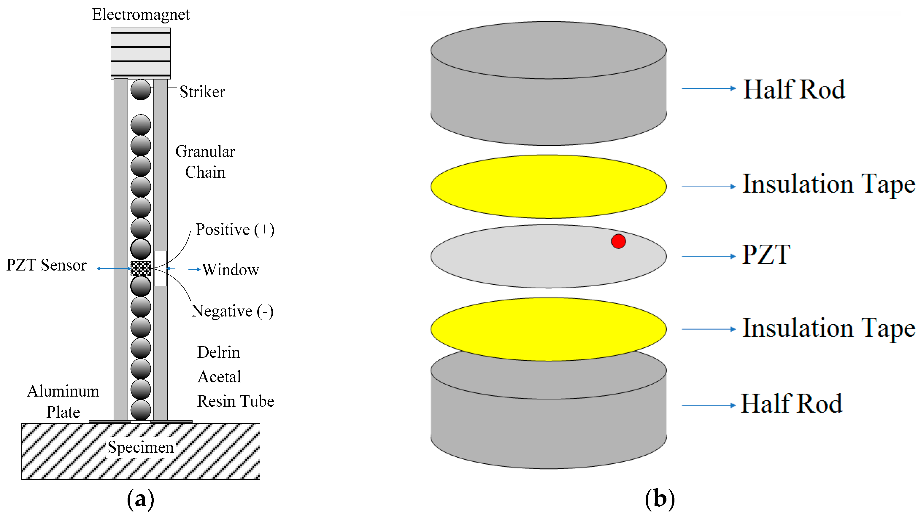
2.2. HNSW Transducers

Three transducers were assembled. Each transducer contained sixteen AISI 302 steel particles (McMaster-Carr, Aurora, IL, USA) as schematized in Figure 3. The second particle from the top was nonferromagnetic, whereas the others were ferromagnetic. The properties of the particles were: diameter d = 19.05 mm, density ρ = 7800 kg/m³, mass m = 27.8 g, modulus of elasticity E = 193 GPa, and Poisson’s ratio ν = 0.29. Each chain was held by a Delrin tube (McMaster-Carr, Aurora, IL, USA) with outer diameter D₀ = 22.30 mm and inner diameter slightly larger than d in order to minimize the friction between the striker and the inner wall of the tube and to minimize acoustic leakage from the chain to the tube. The striker was driven by an electromagnet (made in the lab) built in our lab and powered by a (DC) power supply (B & K Precision, Melrose, MN, USA).

The sensing system consisted of a built-in sensor-rod schematized in Figure 3b and located in lieu of the 9th particle. The sensor-rod was made of a piezo ceramic (Steminc Piezo, Miami, AZ, USA) embedded between two half rods (McMaster-Carr, Aurora, IL, USA). The disc (Steminc Piezo, Miami, AZ, USA) was 19 mm diameter and 0.3 mm thick and insulated with Kapton tape (McMaster-Carr, Aurora, IL, USA). The rod was made from the same material as the beads, and has a mass m_r = 27.8 g, a height h_r = 13.3 mm, and a diameter D_r = 19.05 mm. The sensor-rod had approximately the same mass of the individual particles in order to minimize any impurity in the chain that may generate spurious HNSWs. Finally, the falling height of the striker was 5 mm.

At the bottom of the transducers a 0.254 mm (0.1 in.) thick aluminum sheet (McMaster-Carr, Aurora, IL, USA) was glued to the plastic tube in order to prevent the free fall of the particles. A through-thickness hole was devised to allow for direct contact between the last particle of the chain and the concrete material. The transducers were driven simultaneously by a National Instruments-PXI unit running in LabVIEW (9.0, National Instruments, Austin, TX, USA, 2009), and a DC power supply and a Matrix Terminal Block (NI TB-2643) (National Instruments, Austin, TX, USA) to branch the PXI output into three switch circuits to trigger the action of the electromagnets. The lead-zirconate-titanite (PZT) sensors (Steminc Piezo, Miami, AZ, USA) were connected to the same PXI, and the signals were digitized at 400 kHz sampling frequency, i.e., 2.5 µs sampling period.

2.3. Test Protocol

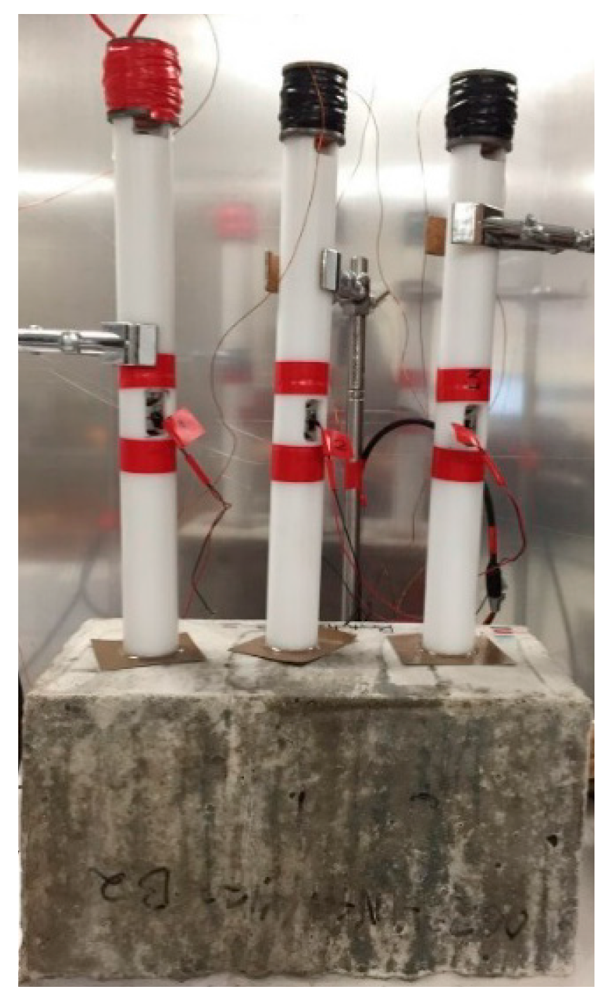
All the HNSW-transducers were used to test all the specimens, i.e., the experiments were conducted in a round-robin fashion, in order to prevent any bias in the results that may have stemmed from differences during the assembly. The cylinders were tested using the HNSWs immediately after curing the samples at 21 °C (70 °F) 95% relative humidity for 28 days, and completed in a day. The experiments were conducted in a single day. For each test, 50 measurements were taken.

The beams were tested at room conditions after 28 days of curing at 21 °C (70 °F) and at relative humidity of 95%. The UPV method was employed the day after testing with the solitary waves. Both top and bottom surfaces of the beams were tested by removing them from the mold and eventually rotated. All the transducers were placed on the surface of the beam simultaneously, and fifty measurements were recorded by each transducer. Figure 4 shows the setups relative to the solitary wave measurements. It can be seen that each sample was tested simultaneously with three transducers and at three different locations. This translates in time and cost-savings. Posts (Techspec, Midland, TX, USA) and clamps (Techspec, Midland, TX, USA) were used to hold the transducers.

2.4. Model to Extract the Elastic Modulus

In order to extract the elastic modulus of the concrete in contact with the chain, we modelled numerically the dynamic interaction between a chain of particles identical to the one embedded in the transducer and an elastic material that mimics the concrete. The partial differential equation of the motion associated with the propagation of an HNSW in the chain can be determined using Lagrangian description of particle dynamics:

$$m{\partial }_{tt}^2{\mu }_n=A{[{\mu }_{n-1}-{\mu }_n]}_{+}^{3/2}-A{[{\mu }_n-{\mu }_{n+1}]}_{+}^{3/2}.$$

(1)

In Equation (1), u_i is the ith particle displacement, [x]₊ denotes max(x, 0), and A the stiffness constant present in the Hertz’s law. By solving this equation, the time history of the nth particle’s oscillation is obtained and then the displacements of the particles can be used to compute the approach δ = u_i+1 − u_i and then to apply in the Hertzian relationship. More details about the models are available at [38,41,42].

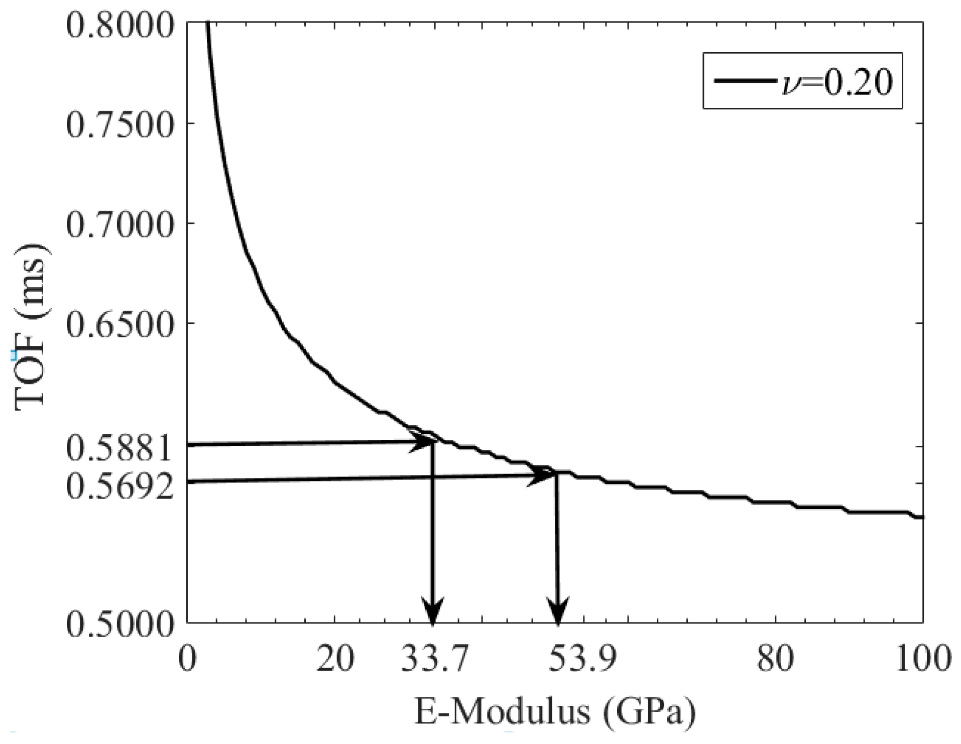
Figure 5 shows the time-of-flight (TOF) of HNSWs as a function of the Young’s modulus for a Poisson’s ratio equal to 0.20, which is a typical value for concrete. The graph shows that the Young’s modulus affects significantly the wave feature when E < 100 GPa; moreover, when the modulus of elasticity of the test sample is higher than 25 GPa, small differences in the measurement of the TOF, let say 3%, yields about 60% change in the estimated modulus. More details about the procedure to generate Figure 5 are available at [43].

In this study, we used Figure 5 to estimate the modulus of the samples by intersecting the experimental TOF to the numerical curve. For illustrative purposes, the figure shows the modulus corresponding to two experimental data, namely 0.5881 ms and 0.5692 ms.

The dynamic modulus of elasticity E_d was then converted into the static modulus of elasticity E_s using the empirical formula proposed by Lydon and Balendran [44,45]:

$$E_s=0.83E_d.$$

(2)

2.5. Ultrasonic Pulse Velocity (UPV) Method

The conventional UPV method was employed for comparative purposes to determine the dynamic modulus of elasticity E_d of the concrete specimens using the well-known relationship:

$$E_d=V^2/K,$$

(3)

where V is the velocity of the bulk wave and K is:

$$K=(1-\mu )/[(1+\mu )(1-2\mu )].$$

(4)

In Equation (4), μ is the dynamic Poisson’s ratio of the sample material. When this ratio is not available, the conventional static Poisson’s ratio ν can be used [1]. After computing the dynamic modulus, Equation (2) is used to estimate the static modulus.

The UPV test was performed by measuring the velocity of the wave propagating along the axial direction of the cylinders, and the through-thickness (top-bottom) direction of the beams. Two commercial transducers (Olympus X1020, 100 kHz, Center Valley, PA, USA), two pre-amplifiers, a function generator (Tektronix AFG 3022, Fort Worth, TX, USA), and an oscilloscope (LeCroy 44 Xi, Chestnut Ridge, NJ, USA) were utilized. The average of 300 measurements was recorded for each cylinder and for each beam.

3. Experimental Results: Baseline Data

3.1. HNSW Transducers and UPV Test

Figure 6a shows one of the fifty waveforms recorded by the transducer P1 when it was placed above the samples 42A, 45A, and 50A. To ease the readability of the time waveforms, the amplitudes were offset. Figure 6b is a close-up view of Figure 6a and it shows that the TOF of the primary reflected wave increases with an increase in w/c ratio. Not presented here, but detailed in [38], the relative standard deviation (RSD), i.e., the ratio of the standard deviation to the mean, ranged from 0.2% to 0.9%. This proved the high repeatability of the setup. The figure reveals that the TOF increases with the increase of the w/c ratio.

The static moduli estimated with Equation (4) are listed in

Table 2. Elastic modulus estimated for the cylinders and based on the time of flight of the reflected wave.

Cylinder	Elastic Modulus (GPa)
	P1	P2	P3	Mean E (GPa) (Per Sample)	Mean (Per w/c Ratio) ± RSD
42A	41.9	41.9	44.7	42.8	41.1% ± 3.38%
42B	41.9	37.0	44.7	41.2
42C	41.9	37.0	39.3	39.4
45A	39.3	39.3	41.9	40.2	37.6% ± 4.82%
45B	39.3	34.9	34.9	36.4
45C	37.0	37.0	34.9	36.3
50A	28.0	33.0	33.0	31.3	31.8% ± 6.00%
50B	28.0	33.0	28.0	29.7
50C	37.0	33.0	33.0	34.3

. They are based on the values of the TOFs averaged from each of the fifty waveforms acquired for every transducer. The values from each transducer and from each cylinder with the same w/c ratio were then averaged and reported on the rightmost column together with the corresponding RSD. The data show that an increase in the w/c ratio decreases the static modulus.

Table 3. Modulus of elasticity estimated for each cylinder and based on the value of the ultrasonic velocity of the longitudinal wave propagating along the cylinder axial direction.

Cylinder	Wave Speed (m/s)	Elastic Modulus (GPa)	Mean Elastic Modulus (GPa) (Per w/c Ratio) ± RSD
42A	4692	34.4	34.9% ± 1.43%
42B	4730	34.8
42C	4740	35.6
45A	4340	31.8	31.8% ± 0.90%
45B	4456	32.1
45C	4407	31.4
50A	4367	29.6	29.5% ± 0.64%
50B	4344	29.6
50C	4330	29.2

presents instead the results associated with the UPV. When compared to the HNSW-based data, the ultrasonic test gives lower modulus and smaller RSD. The latter is due to the better repeatability of the commercial transducer, but it is also the effect of the fact that the ultrasonic test averages the effect of the through-thickness concrete. Finally, it must be noticed that the presence of an ultrasonic gel couplant between the transducer and the concrete mitigates any effect associated with the surface texture.

3.2. Destructive Testing

As is said in Section 2.1, three specimens from each batch were tested according to C469. This standard is traditionally followed to estimate the static modulus of elasticity. The results are presented in

Table 4. Modulus of elasticity estimated using ASTM C469.

Sample	Elastic Modulus (GPa)	Mean (Per w/c Ratio) ± RSD
C42D	40.1	38.6% ± 3.29%
C42E	37.0
C42F	38.8
C45D	36.2	35.7% ± 4.51%
C45E	32.4
C45F	35.2
C50D	32.6	32.4% ± 1.33%
C50E	31.8
C50F	32.8

. Interestingly, the values of the elastic moduli are closer to those predicted with the HNSWs whereas the UPV data underestimated the elastic properties of the cylinders. Nonetheless, the destructive testing confirmed that the modulus of elasticity decreased with an increase in the w/c ratio. On average, the moduli relative to the w/c = 0.45 samples and the w/c = 0.50 samples were 7.5% and 9.2%, respectively, smaller than the w/c = 0.42 sample.

4. Experimental Results: Short Beams

Table 2, Table 3 and Table 4 constitute the reference data to which compare the findings from the corrupted beams. The results are presented in what follows.

4.1. HNSW-Transducer Measurements

Figure 7a–d show one of the fifty waveforms recorded by the transducer P1 when it was placed above the beams with water in excess. To ease the readability of the time waveforms, the amplitudes were offset. Figure 7e–h are the close-up view of Figure 7a–d, and they reveal some variation in the TOF between the pristine and the conditioned samples. In what follows, the time waveforms are analyzed to validate the hypothesis that the differences are due to the presence of unwanted water.

Table 5. Time of flight and modulus of elasticity of the beams in which Condition 1 was imposed.

Cast Day	Sample	Top		Bottom
		TOF (ms)	E (GPa)	TOF (ms)	E (GPa)
Day 1	1	0.59224	27	0.57640	37
		0.60296	21	0.58092	33
		0.60428	21	0.57044	42
	2	0.59316	25	0.58244	33
		0.58156	33	0.58072	33
		0.59200	27	0.57508	37
Day 2	3	0.58536	30	0.58364	31
		0.57764	35	0.57880	35
		0.57624	37	0.57728	37
	4	0.57892	35	0.56896	45
		0.60128	22	0.58384	31
		0.56924	45	0.58648	30
Average E (GPa) Short beam w/c = 0.42		29.83 ± 7.08 (23.73%)		35.33 ± 4.37 (12.35%)
Cylinder w/c = 0.42		41.1 ± 1.389 (3.38%)
Cylinder w/c = 0.45		37.6 ± 1.815 (4.82%)
Cylinder w/c = 0.50		31.8 ± 1.907 (6.00%)

summarizes the results associated with the beam subject to Condition 1, i.e., with the presence of 12.7 mm (0.5 in.) of standing water at the bottom of the formwork. The average value of the fifty TOF measurements per transducer is listed along with the corresponding elastic modulus. The data refer to the beam both top and bottom face. The latter was exposed to the presence of water. However, as is said earlier and displayed in Figure 2a, water migrated toward the top due to vibration and the weight of the concrete. The mean of the twelve moduli is presented in the shaded row along with the corresponding standard deviation and RSD. Surprisingly, the modulus estimated at the top surface is higher than the modulus at the bottom where the standing water was originally located. The results are therefore consistent with the empirical evidence that water migrated to the top and the experimental procedure that water was mixed with the concrete throughout the specimen. The RSD associated with the measurement at the top is almost double the corresponding value at the bottom. This is the result of point-by-point variations due to the presence of water whereas the conditions at the bottom were more uniform due to the self-weight of the concrete and the smoothness of the mold. We will observe that this consideration about the RSD applies to all four conditions.

The last three rows of Table 5 list the elastic modulus of the baseline cylinders predicted by the same transducers. They are presented here again to ease the prediction of the resulting w/c ratio at the two surfaces of the beams. By comparing the values relative to the beams and to the cylinders, the solitary wave based technique estimates a ratio higher than 0.50 at the top and around 0.46–0.47 at the bottom of the short beams.

Similar to Table 5,

Table 6. Time of flight and modulus of elasticity of the beams in which Condition 2 was imposed.

Cast Day	Sample	Top		Bottom
		TOF (ms)	E (GPa)	TOF (ms)	E (GPa)
Day 1	1	0.58332	31	0.57592	37
		0.60476	21	0.57420	39
		0.58260	31	0.56976	45
	2	0.60224	22	0.56684	48
		0.58900	28	0.58128	33
		0.60460	21	0.57644	37
Day 2	3	0.58320	31	0.59280	25
		0.59096	27	0.58152	33
		0.57112	42	0.57180	42
	4	0.57972	35	0.57800	35
		0.57908	35	0.58512	30
		0.58492	31	0.57236	42
Average E (GPa) Short beam w/c = 0.42		29.58 ± 6.02 (20.35%)		37.17 ± 6.24 (16.80%)
Cylinder w/c = 0.42		41.1 ± 1.389 (3.38%)
Cylinder w/c = 0.45		37.6 ± 1.815 (4.82%)
Cylinder w/c = 0.50		31.8 ± 1.907 (6.00%)

presents the results relative to Condition 2 where the amount of standing water was half the amount in Condition 1. By looking at the mean of the elastic modulus, we observe that the value relative to the top surface is very close to the value reported in Table 5, whereas the w/c ratio estimated at the bottom is 0.45. The results suggest that the difference in the amount of standing water between Conditions 1 and 2 was not relevant to change the w/c ratio of the overall beam. By looking at the three bottommost rows of Table 6, we can reach the same conclusions for both conditions: the HNSW transducers were able to capture the circumstance that the short beams were corrupted by water in excess.

The TOF and the static modulus at the surfaces of the beams experiencing Condition 3 are summarized in

Table 7. Time of flight and modulus of elasticity of the beams in which Condition 3 was imposed.

Cast Day	Sample	Top		Bottom
		TOF (ms)	E (GPa)	TOF (ms)	E (GPa)
Day 1	1	0.57672	37	0.57420	39
		0.58312	31	0.57420	39
		0.57660	37	0.57888	35
	2	0.57164	42	0.56576	48
		0.59256	25	0.57420	39
		0.57924	35	0.57292	39
Day 2	3	0.59048	27	0.57600	37
		0.57988	35	0.57200	42
		0.58828	28	0.57400	39
	4	0.58448	31	0.57872	35
		0.59096	27	0.57000	42
		0.59000	27	0.57600	37
Average E (GPa) Short beam w/c = 0.42		31.83 ± 5.07 (15.96%)		39.25 ± 3.394 (8.650%)
Cylinder w/c = 0.42		41.1 ± 1.389 (3.38%)
Cylinder w/c = 0.45		37.6 ± 1.815 (4.82%)
Cylinder w/c = 0.50		31.8 ± 1.907 (6.00%)

. Under this scenario, 2.54 mm (0.1 in.) of water was sprinkled above the samples, whereas the bottom surface was pristine with w/c = 0.42 (see scheme of Figure 1c). It is observed that the estimated static modulus for the top surface is 31.8 GPa and it matches the cylinders with w/c = 0.50. When compared to the corresponding values presented in Table 5 and Table 6, the modulus is slightly higher, and this is likely because the volume of water sprinkled on the samples was lower. Moreover, the value is much smaller than the modulus of elasticity estimated for the cylinders with w/c = 0.42. The elastic modulus measured at the bottom surface was higher than the previous two scenarios; this is expected since the specimens with Conditions 3 and 4 were not vibrated, and, therefore, it is unlikely that the water sprinkled on the top reached the bottom of the specimen.

Finally, the TOF and the modulus of elasticity of the beams subjected to Condition 4 are summarized in

Table 8. Time of flight and modulus of elasticity of the beams in which Condition 4 was imposed.

Cast Day	Sample	Top		Bottom
		TOF (ms)	E (GPa)	TOF (ms)	E (GPa)
Day 1	1	0.59608	24	0.57420	39
		0.58260	31	0.57420	39
		0.57944	35	0.57768	35
	2	0.59276	25	0.57644	37
		0.58484	31	0.57668	37
		0.59608	24	0.57420	39
Day 2	3	0.57892	35	0.57401	39
		0.57768	35	0.57200	42
		0.58492	31	0.57800	35
	4	0.58932	28	0.57600	37
		0.58512	30	0.56740	48
		0.57172	42	0.57600	37
Average E (GPa) Short beam w/c = 0.42		30.92 ± 5.107 (16.52%)		38.67 ± 3.37 (8.73%)
Cylinder w/c = 0.42		41.1 ± 1.389 (3.38%)
Cylinder w/c = 0.45		37.6 ± 1.815 (4.82%)
Cylinder w/c = 0.50		31.8 ± 1.907 (6.00%)

. Under this condition, more water was added onto the fresh concrete. Consistently with the larger volume of liquid, the predicted modulus at the top was lower than what estimated under scenario 3. The table demonstrates that the HNSW-based measurement estimated that the w/c of the unconditioned surface of the concrete beam was close to 0.42, as it is expected, and above 0.50 for the surface of the beam that was sprinkled with 3.8 mm (0.15 in) of water. It is noted here that sampling period used in this study and the design of the metamaterial are such that the potential error in the estimate of the concrete modulus is on the order of 5%. The accuracy can be improved by simply increasing the sapling frequency of the digitizer. Nonetheless, the outcomes of the results are in line with the prediction of water in excess in the concrete beams.

4.2. UPV Test

UPV was adopted to test the beams as well. The results are summarized in

Table 9. The modulus of elasticity of the beams in which different conditions are measured by UPV (ultrasonic pulse velocity) test.

Condition	E (GPa) Mean ± Standard Deviation	RSD (%)
1	31.44 ± 0.966	3.07
2	31.13 ± 1.558	5.00
3	32.37 ± 1.354	4.18
4	29.42 ± 2.660	9.04

. The means of the modulus are much closer to each other than what was found with the HNSW method. This remarks upon the fact that the novel NDE method is capable of capturing surface conditions that may have been altered by the presence of water. Moreover, the RSD is smaller, suggesting more homogeneous conditions throughout the four samples. Finally, if we compare the UPV data from Table 4 and Table 9, we notice that the UPV method estimates an amount of w/c ratio above 50% for all samples, without any ability at discriminating poor from good surface conditions.

5. Discussion and Conclusions

In this article, we showed the principles of a novel NDE method for concrete based on the propagation of highly nonlinear solitary waves along a metamaterial in contact with the concrete to be evaluated. The method aimed at determining the modulus of hardened concrete, in particular to estimate the water-to-cement ratio in a concrete volume close to an HNSW transducer. We demonstrated that the transducers designed and assembled to exploit the principles offer sufficient repeatability and reliability to identify the differences in the amount of water purposely added to the beams in order to mimic rainfall situations.

Owing to the nature of concrete material, it is acknowledged that the w/c ratio is likely not to be the only concrete parameter affecting the amplitude and the time of flight of the reflected solitary wave. Future studies should look at the effect of the aggregate size and overall any other factor that is known to influence the Young’s modulus of concrete. Nonetheless, the study presented in this paper is the first attempt to prove that solitary waves can be used to measure water in excess in concrete surfaces.

The advantages of the proposed HNSW-based method are the easy and fast implementation, the possibility to carry out a large number of tests simultaneously, and independence upon internal damage and/or the presence of reinforcing steels inside the concrete. Finally, being a local and contact method, the approach can be successfully applied to characterizing effects of finishing and curing conditions.

Figure 5 showed that the measured values of E are on a part of the curve that is not extremely favorable for sensitivity. Future studies should redesign the metamaterial, such as different sized or different modulus balls, in order to shift the region of influence in a range where a large change in the TOF gives rise to small variation of the Young modulus. Such a region would consent to discriminate small differences in the Young modulus due to changes in the w/c ratio.

References

1. Malhotra, V.M.; Carino, N.J. Handbook on Nondestructive Testing of Concrete Second Edition; CRC Press: Boca Raton, FL, USA, 2003. [Google Scholar]
2. Karaiskos, G.; Deraemaeker, A.; Aggelis, D.; van Hemelrijck, D. Monitoring of concrete structures using the ultrasonic pulse velocity method. Smart Mater. Struct. 2015, 24. [Google Scholar] [CrossRef]
3. Shah, A.; Ribakov, Y.; Zhang, C. Efficiency and sensitivity of linear and non-linear ultrasonics to identifying micro and macro-scale defects in concrete. Mater. Des. 2013, 50, 905–916. [Google Scholar] [CrossRef]
4. Ye, G.; Lura, P.; van Breugel, K.; Fraaij, A. Study on the development of the microstructure in cement-based materials by means of numerical simulation and ultrasonic pulse velocity measurement. Cem. Concr. Compos. 2004, 26, 491–497. [Google Scholar] [CrossRef]
5. Lin, Y.; Lai, C.-P.; Yen, T. Prediction of ultrasonic pulse velocity (UPV) in concrete. ACI Mater. J. 2003, 100, 21–28. [Google Scholar]
6. Shariq, M.; Prasad, J.; Masood, A. Studies in ultrasonic pulse velocity of concrete containing GGBFS. Constr. Build. Mater. 2013, 40, 944–950. [Google Scholar] [CrossRef]
7. Komlos, K.; Popovics, S.; Nürnbergerova, T.; Babal, B.; Popovics, J. Ultrasonic pulse velocity test of concrete properties as specified in various standards. Cem. Concr. Compos. 1996, 18, 357–364. [Google Scholar] [CrossRef]
8. Popovics, S. Analysis of the concrete strength versus ultrasonic pulse velocity relationship. Mater. Eval. 2001, 59, 123–130. [Google Scholar]
9. Hong, S.; Cho, Y.; Kim, S.; Lee, Y. Estimation of compressive strength of concrete structures using the ultrasonic pulse velocity method and spectral analysis of surface wave method. Mater. Res. Innov. 2015, 19. [Google Scholar] [CrossRef]
10. Huang, Q.; Gardoni, P.; Hurlebaus, S. Predicting concrete compressive strength using ultrasonic pulse velocity and rebound number. ACI Mater. J. 2011, 108, 403–412. [Google Scholar]
11. ASTM (American Society for Testing Material) C805/C805m-08. Standard Test Method for Rebound Number of Hardened Concrete; ASTM: West Conshohocken, PA, USA, 2008. [Google Scholar]
12. Borosnyói, A. NDT assessment of existing concrete structures: Spatial analysis of rebound hammer results recorded in-situ. E. Struct. Technol. 2015, 7, 1–12. [Google Scholar] [CrossRef]
13. Cano-Barrita, P.D.J.; Castellanos, F.; Ramírez-Arellanes, S.; Cosmes-López, M.; Reyes-Estevez, L.; Hernández-Arrazola, S.; Ramírez-Ortíz, A. Monitoring compressive strength of concrete by nuclear magnetic resonance, ultrasound, and rebound hammer. ACI Mater. J. 2015, 112, 147–154. [Google Scholar] [CrossRef]
14. Proceq. Available online: http://www.Proceq.Com/products/concrete-testing/concrete-test-hammer/original-schmidt (accessed on 10 January 2016).
15. Choi, H.; Popovics, J.S. Nde application of ultrasonic tomography to a full-scale concrete structure. IEEE Trans. Ultrason. Ferroelectr. Freq. Control 2015, 62, 1076–1085. [Google Scholar] [CrossRef] [PubMed]
16. Völker, C.; Shokouhi, P. Multi sensor data fusion approach for automatic honeycomb detection in concrete. NDT E Int. 2015, 71, 54–60. [Google Scholar] [CrossRef]
17. Kim, G.; In, C.-W.; Kim, J.-Y.; Kurtis, K.E.; Jacobs, L.J. Air-coupled detection of nonlinear rayleigh surface waves in concrete—Application to microcracking detection. NDT E Int. 2014, 67, 64–70. [Google Scholar] [CrossRef]
18. Saravanan, T.J.; Balamonica, K.; Priya, C.B.; Reddy, A.L.; Gopalakrishnan, N. Comparative performance of various smart aggregates during strength gain and damage states of concrete. Smart Mater. Struct. 2015, 24. [Google Scholar] [CrossRef]
19. Clayton, D.A.; Barker, A.M.; Santos-Villalobos, H.J.; Albright, A.P.; Hoegh, D.K.; Khazanovich, D.L. Nondestructive Evaluation of Thick Concrete Using Advanced Signal Processing Techniques; Oak Ridge National Laboratory (ORNL): Oak Ridge, TN, USA, 2015. [Google Scholar]
20. Shih, Y.-F.; Wang, Y.-R.; Lin, K.-L.; Chen, C.-W. Improving non-destructive concrete strength tests using support vector machines. Materials 2015, 8, 7169–7178. [Google Scholar] [CrossRef]
21. Amini, K.; Jalalpour, M.; Delatte, N. Advancing concrete strength prediction using non-destructive testing: Development and verification of a generalizable model. Constr. Build. Mater. 2016, 102, 762–768. [Google Scholar] [CrossRef]
22. Saleem, M.; Al-Kutti, W.A.; Al-Akhras, N.M.; Haider, H. Nondestructive testing procedure to evaluate the load-carrying capacity of concrete anchors. J. Constr. E. Mang. 2015. [Google Scholar] [CrossRef]
23. Pucinotti, R. Reinforced concrete structure: Non destructive in situ strength assessment of concrete. Constr. Build. Mater. 2015, 75, 331–341. [Google Scholar] [CrossRef]
24. Azari, H.; Nazarian, S. Optimization of acoustic methods for condition assessment of concrete structures. ACI Mater. J. 2015, 112. [Google Scholar] [CrossRef]
25. Ham, S.; Popovics, J.S. Application of micro-electro-mechanical sensors contactless NDT of concrete structures. Sensors 2015, 15, 9078–9096. [Google Scholar] [CrossRef] [PubMed]
26. Hoegh, K.; Khazanovich, L.; Dai, S.; Yu, T. Evaluating asphalt concrete air void variation via GPR antenna array data. Case Stud. Nondestruct. Test. Eval. 2015, 3, 27–33. [Google Scholar] [CrossRef]
27. Iliopoulos, S.N.; Aggelis, D.G.; Polyzos, D. Wave dispersion in fresh and hardened concrete through the prism of gradient elasticity. Int. J. Solids Struct. 2016, 78, 149–159. [Google Scholar] [CrossRef]
28. Dimter, S.; Rukavina, T.; Minažek, K. Estimation of elastic properties of fly ash–stabilized mixes using nondestructive evaluation methods. Constr. Build. Mater. 2016, 102, 505–514. [Google Scholar] [CrossRef]
29. Hertz, H. On the contact of elastic solids. J. Reine Angew. Math. 1881, 92, 156–171. [Google Scholar]
30. Nesterenko, V.F. Dynamics of Heterogeneous Materials; Springer Science & Business Media: Berlin, Germany, 2013. [Google Scholar]
31. Li, F.; Zhao, L.; Tian, Z.; Yu, L.; Yang, J. Visualization of solitary waves via laser doppler vibrometry for heavy impurity identification in a granular chain. Smart Mater. Struct. 2013, 22. [Google Scholar] [CrossRef]
32. Boechler, N.; Yang, J.; Theocharis, G.; Kevrekidis, P.; Daraio, C. Tunable vibrational band gaps in one-dimensional diatomic granular crystals with three-particle unit cells. J. Appl. Phys. 2011, 109. [Google Scholar] [CrossRef]
33. Ni, X.; Rizzo, P.; Daraio, C. Laser-based excitation of nonlinear solitary waves in a chain of particles. Phys. Rev. E 2011, 84. [Google Scholar] [CrossRef] [PubMed]
34. Herbold, E.B. Optimization of The Dynamic Behavior of Strongly Nonlinear Heterogeneous Materials. Ph.D. Thesis, University of California, San Diego, CA, USA, 2008. [Google Scholar]
35. Daraio, C.; Nesterenko, V.F.; Herbold, E.; Jin, S. Tunability of solitary wave properties in one-dimensional strongly nonlinear phononic crystals. Phys. Rev. E 2006, 73. [Google Scholar] [CrossRef] [PubMed]
36. Carretero-González, R.; Khatri, D.; Porter, M.A.; Kevrekidis, P.; Daraio, C. Dissipative solitary waves in granular crystals. Phys. Rev. Let. 2009, 102. [Google Scholar] [CrossRef] [PubMed]
37. Porter, M.A.; Daraio, C.; Szelengowicz, I.; Herbold, E.B.; Kevrekidis, P. Highly nonlinear solitary waves in heterogeneous periodic granular media. Phys. D Nonlinear Phenom. 2009, 238, 666–676. [Google Scholar] [CrossRef]
38. Nasrollahi, A.; Deng, W.; Rizzo, P.; Vuotto, A.; Vandenbossche, J.M.; Li, K. University of Pittsburgh: Pittsburgh, PA, USA, Unpublished work. 2016.
39. Ni, X.; Rizzo, P.; Yang, J.; Katri, D.; Daraio, C. Monitoring the hydration of cement using highly nonlinear solitary waves. NDT E Int. 2012, 52, 76–85. [Google Scholar] [CrossRef]
40. Rizzo, P.; Ni, X.; Nassiri, S.; Vandenbossche, J. A solitary wave-based sensor to monitor the setting of fresh concrete. Sensors 2014, 14, 12568–12584. [Google Scholar] [CrossRef] [PubMed]
41. Herbold, E.; Kim, J.; Nesterenko, V.; Wang, S.; Daraio, C. Pulse propagation in a linear and nonlinear diatomic periodic chain: Effects of acoustic frequency band-gap. Acta Mech. 2009, 205, 85–103. [Google Scholar] [CrossRef]
42. Yang, J.; Silvestro, C.; Khatri, D.; de Nardo, L.; Daraio, C. Interaction of highly nonlinear solitary waves with linear elastic media. Phys. Rev. E 2011, 83. [Google Scholar] [CrossRef] [PubMed]
43. Bagheri, A.; Rizzo, P.; Al-Nazer, L. A numerical study on the optimization of a granular medium to infer the axial stress in slender structures. Mech. Adv. Mat. Struct. 2016, 23, 1131–1143. [Google Scholar] [CrossRef]
44. Lydon, F.; Balendran, R. Some observations on elastic properties of plain concrete. Cem. Concr. Res. 1986, 16, 314–324. [Google Scholar] [CrossRef]
45. Popovics, J.; Zemajtis, J.; Shkolnik, I. ACI-CRC Final Report. In A Study of Static and Dynamic Modulus of Elasticity of Concrete; Civil and Environmental Engineering, University of Illinois: Urbana, IL, USA, 2008. [Google Scholar]
Figure 1. Schematics of the four conditions simulated on the 152.4 × 152.4 × 254 mm3 concrete beams. (a) Condition 1 in which 12.7 mm of water sits at the bottom of the form mimicking standing water on the formwork before concreting; (b) Condition 2 in which 6.35 mm of water sits at the bottom of the form mimicking standing water on the formwork before concreting; (c) Condition 3 in which 2.54 mm of water is sprinkled at the top of the beam mimicking rainfall during concreting; (d) Condition 4 in which 3.81 mm of water is sprinkled at the top of the beam mimicking rainfall during concreting.
Applsci 06 00104 g001
Figure 2. Photos of the preparation of the samples. (a) close-up view of one of the samples under Condition 2; standing water from bottom of beam mold migrates to the top; (b) preparation of one of the samples under Condition 3: finishing beam surface after second application of water; (c) rodding the same sample shown in (b) during the third and final application of surface water.
Applsci 06 00104 g002
Figure 3. (a) scheme of the solitary waves based transducers used in this study (b) assembly of the sensor-rod inserted in the transducers.
Applsci 06 00104 g003
Figure 4. Photo of the three transducers during the experiment.
Applsci 06 00104 g004
Figure 5. Numerical results: time of flight (TOF) as a function of the dynamic modulus of elasticity when the material in contact with the chain of spherical particles has Poisson’s ratio ν = 0.20.
Applsci 06 00104 g005
Figure 6. HNSW (highly nonlinear solitary wave)-based measurement using the transducers. (a) time waveform relative to P1 for the cylinders with different w/c ratio; (b) close-up view of panel (a).
Applsci 06 00104 g006
Figure 7. The time waveforms and their close up views obtained from the short beam tests: (a) condition 1; (b) condition 2; (c) condition 3; and (d) condition 4; (e), (f), (g), and (h) are the close views of (a), (b), (c), and (d), respectively.
Applsci 06 00104 g007