Thermal Energy Storage for Building Load Management: Application to Electrically Heated Floor

Abstract

In cold climates, electrical power demand for space conditioning becomes a critical issue for utility companies during certain periods of the day. Shifting a portion or all of it to off-peak periods can help reduce peak demand and reduce stress on the electrical grid. Sensible thermal energy storage (TES) systems, and particularly electrically heated floors (EHF), can store thermal energy in buildings during the off-peak periods and release it during the peak periods while maintaining occupants’ thermal comfort. However, choosing the type of storage system and/or its configuration may be difficult. In this paper, the performance of an EHF for load management is studied. First, a methodology is developed to integrate EHF in TRNSYS program in order to investigate the impact of floor assembly on the EHF performance. Then, the thermal comfort (TC) of the night-running EHF is studied. Finally, indicators are defined, allowing the comparison of different EHF. Results show that an EHF is able to shift 84% of building loads to the night while maintaining acceptable TC in cold climate. Moreover, this system is able to provide savings for the customer and supplier if there is a significant difference between off-peak and peak period electricity prices.

1. Introduction

In cold climate, intense energy consumption periods during winter [1] compels utility providers to meet the demand with peaking power plants (usually using fossil fuel) and/or by purchasing the electricity at high prices from the market. Thus, from environmental, economical and technical (grid congestion) points of view, it is necessary to shift the peak demand to the off-peak periods.

Several techniques have been suggested for shifting peak load. One approach is to encourage users to shift their consumption themselves. Some countries implement price scales depending on the time period: peak periods (higher cost) or off-peak periods (lower cost). The goal is to financially encourage users to use electricity during off-peak periods. There are several types of price scales: with only two periods per day (“Time of use”); with a higher price only when the grid is stressed (“Critical peak pricing”) or with a variable price every hour depending on the real price in the electricity market [2]. Several studies used these price scales to decrease peak consumption [3,4,5].

Thus, to decrease peak period consumption, the use of storage systems, which will store energy during off-peak periods and release it during peak periods, is studied. The building envelope, central heating system, and hot water tank are already used as thermal energy storage (TES) [6,7,8,9,10].

One approach is to use the thermal mass of the building envelope, especially in integrating the heating system in the floor assembly using a hydronic floor heating system or an electrically heated floor (EHF). Benefits of floor heating systems are numerous; heating elements are installed within the floor assembly and therefore are invisible to the occupants in the building. Moreover, thermal radiation could provide a better thermal comfort (TC) for the occupants if the floor surface temperature stays below 29 °C [11]. In fact, using a radiative heating system in comparison to a convective heating system allows diminishing the forced air-circulating loop in the room and the heat sensation will be higher for people with the same indoor temperature. Thus, the possibility to have a lower indoor temperature with the same thermal comfort to reduce the energy consumption of the building (18% in the study of Ghali [12]). Moreover, in comparison to hydronic system, the addition of a hot water tank is not necessary and maintenance is almost non-existent for electrically heated floor.

Floor heating systems have been used in previous studies to reduce the peak energy consumption. Kattan et al. [13] reported that a hydronic floor heating system could reduce the load by 26% during the peak periods and the total energy consumption by 30% in comparison to a conventional convective system. Li et al. [14] investigated a number of control strategies for shifting the peak demand while the heating system was allowed to operate between 8:00 p.m. and 6:00 a.m., unless the TC was jeopardized. Their results showed that there is an 80% load reduction during the peak period. However, the simulation was carried out during office hours, thus the TC was only studied between 8:00 a.m. and 6:00 p.m. Moreover, the study did not report the floor surface temperature (FST).

Lin et al. [15] carried out an experiment with an EHF integrated with PCM in an environment with an average outdoor temperature of 13.6 °C. The system did not operate from 8:00 a.m. to 11:00 p.m. During the night, their control strategy was based on the heating element temperature (heaters stopped working when the heater temperature was over 70 °C and worked again when it was below 55 °C). It was found that the system did not have a good control over the room and floor surface temperatures, which resulted in high average indoor temperature (31 °C) and FST (40 °C). Cheng et al. [16] conducted simulations and experiments with an EHF with a shape-stabilized PCM. The heating time lasted 10 hours and the intermittent time lasted 14 hours, with outdoor temperature between 0 °C and 6 °C. In comparison with other heating strategies (i.e., operating all day), the EHF with PCMs was able to completely shift the load from peak periods to off-peak periods. Nevertheless, average room temperatures were quite low (between 15 °C and 16 °C). Thus, the TC requirements were not met.

The results of the earlier investigations show that a floor heating system is able to shift part of or the entire space-conditioning load from peak periods to off-peak periods, but it may not be able to provide the required TC, especially with intermittent heating mode. Moreover, the performance of the system in cold climate regions has not been thoroughly investigated, and the majority of studies were conducted using hydronic floor heating systems. To improve the performance of the floor heating system, it is important to understand the behavior and the importance of each layer of the assembly on the performance of EHF. First, the insulation layer between the ground and the floor heating system has a considerable influence on the floor heating system performance. Previous studies reported that a thicker insulation layer is required to reduce heat losses to the ground for a floor heating system compared to a conventional system [17,18]. Moreover, the effect of the concrete thickness on the performance of the system has also been studied. With a hydronic floor heating system with concrete, Wang et al. [19] reported the impact of the concrete layer on the performance of hydronic heating system: the floor surface temperature is higher when the concrete layer is thin.

However, the behavior of each layer of a floor heating system with the aim of storing energy with high slab temperature variations was not thoroughly investigated. Therefore, further investigation is necessary for EHF with the objective of completely/partly shifting the peak demand to off-peak hours while maintaining the occupants’ TC. To realize this, the software TRNSYS (version 17 [20]) is used to model the building. However, the existing models for an EHF in TRNSYS do not allow the consideration of the thermal mass on the top of the EHF. Thus, a procedure is developed for the integration of an EHF in TRNSYS. Then, the developed model is used to study the ability of the EHF to shift part of or the entire load of the peak period in a cold climate. Consequently, the influence of each layer of the EHF is investigated with a parametric study. Then, the thermal comfort in the building is studied with the EHF when it is charged during the night only (off-peak period). Finally, some indicators are developed to compare the EHF with other EHF or sensible TES systems.

2. Materials and Methods

In this section, the methodology to integrate the EHF in TRNSYS is presented. Then, procedures to realize the parametric study, the thermal comfort examination and the adaptation of indicators are presented.

2.1. EHF in TRNSYS

2.1.1. Existing Methodologies for EHF in TRNSYS

TRNSYS is the abbreviation for TRaNsient SYStems simulation program. This software works with modules called “types”. The types are mathematical models, in which users can choose to link inputs and outputs of different types together in order to study the performance of a system. The format of the program makes this software very flexible. Type 56 is used to study the thermal behavior of a multi-zone building [20]. This type allows the modeling of the complex behavior of a building, taking into consideration many geometric parameters (thicknesses, surfaces, positions of zones, etc.), but also weather data and occupancy schedule.

Type 56 was used to simulate a residential building. The simulation was validated with measured field data [21]. For this study, the building was modified to meet the requirements of this project: the existing heating systems (electric baseboard) were replaced by EHFs. To model the EHF in TRNSYS, two methods can be used.

The first method is the use of the wall gain: the wall gain is defined as “an energy flux to the inside wall surface”. Considering that the name “wall” in TRNSYS is used whether it is positioned as an actual wall, floor or roof, the wall gain is thus analogous to simply defining a given heat flux on a surface. However, the wall gain can only be defined on the top of the surface and not within it, and consequently may change the storage system behavior.

Another possibility is to use the active layer, which is designed for hydronic floor heating systems. By choosing a high water flow rate, a constant water temperature can be assumed: it can then behave as an EHF. Nevertheless, the use of the active layer requires the determination of the relationship between the parameters of the active layer (flow, pipe diameter, pipe conductivity, water temperature, etc.) and the EHF power. Moreover, to use this type of layer, some hypotheses have to be verified [22], which may limit the parametric study.

For this study, the wall gain method is selected, with some modifications to go beyond the presented limit.

2.1.2. Integration of EHF

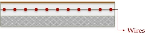
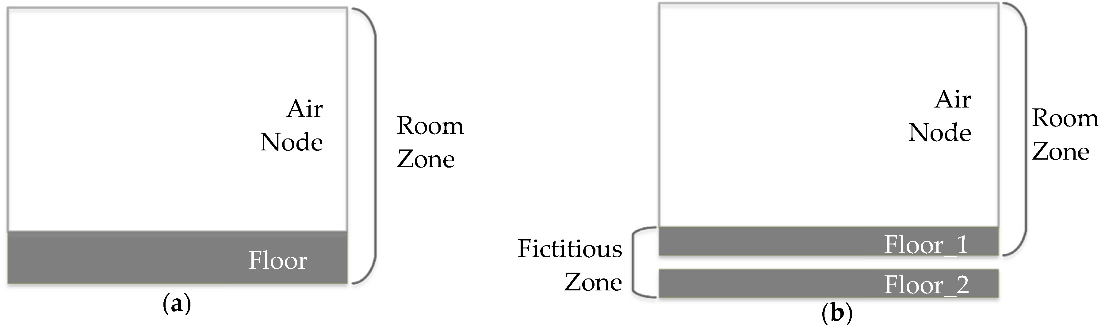
Some modifications must be made in the floor assembly in order to use the wall gain to model the building integrated with an EHF. In an EHF, heating elements are uniformly placed within the concrete. Thus, the power is evenly distributed and the concept of constant power gain can be applied to EHF. Then, to model the heat flux, a wall gain was used. To apply this surface gain for such application, a fictitious zone was created below the room zone, as presented in Figure 1. By having the size of the air volume of this fictitious zone infinitesimally small and assuming a high heat transfer coefficient for the fictitious zone, a perfect contact between two layers can be assumed. In addition, the perimeter heat losses were neglected since the height of the air node of the fictitious zone is very small.

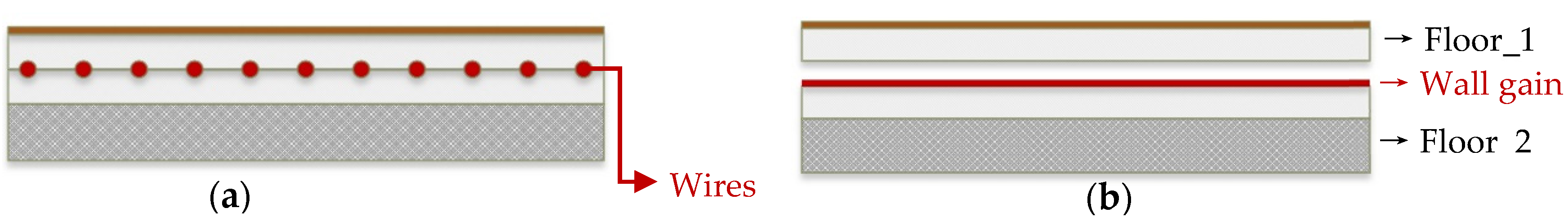
This fictitious zone has one floor (connected to the ground) and one ceiling (connected to the room zone), see Figure 1. Coupled together, these two zones represent all layers of the floor assembly. The wall gain, used as a surface gain (the EHF), is added on the upper-surface of the lower-wall (between the Floor_1 and Floor_2, see Figure 2) to model the wires. The total thickness of each material (insulation, concrete and plywood) is the same in the two configurations.

2.1.3. Model Verification

The implementation of this model was applied to a residential building in Montreal (QC, Canada), which had been previously validated for electric baseboard with field measurement data [21] and used in previous studies [22]. To validate the model, the main consideration was to be sure that the creation of a new zone “fictitious” was done properly and the proposed wall gain approach simulates the behavior of the system accurately.

To validate the integration of the fictitious zone, the wall gain was set to zero, and electrical baseboards were used to heat the building with the same control strategy as the one used earlier [21] (operating all day as function of the indoor temperature with a set-point at 21 °C). Simulations were performed for one month (in January), for the reference building (equipped with electrical baseboards only) and the modified one (with electrical baseboards and with the EHF structure with the wall gain set to 0). The energy consumption of the two heating systems were then compared in calculating the Normalized Mean Bias Error (NMBE). Details on the calculation of this statistical index are accessible on the ASHRAE Guideline 14-2014 [23]. Results are presented in

Table 1. Statistical index to compare energy consumptions of the reference building and the modified one.

Statistical index	Monthly	Hourly
NMBE	0.20%	1.91%

. The passive EHF model is shown not to have adversely affected the building performance.

To validate the assumption of perfect contact between the two concrete layers, the temperature on the bottom of Floor_1 was compared to the temperature on the top of Floor_2 (see Figure 2). These temperatures are outputs of TRNSYS. The temperature difference between the upper side of Floor_2 and the lower side of Floor_1 was calculated for 10 days, and only the last eight days were taken for analysis (to ignore the initial condition effect): results showed a NMBE of less than 1%.

Finally, Olsthoorn et al. [24] modeled the same EHF using 2D finite-element analysis. Their results are very close to the 1D TRNSYS model results presented in this paper: the predicted temperature at the heating cable height from the TRNSYS model was 32.38 °C, when the average temperature on the 2D model of was 31.11 °C. Similarly, results of the 2D model show a difference in the floor surface temperature in comparison with the TRNSYS model of approximately 1 °C. Moreover, the hypothesis of an isothermal floor surface was validated.

2.1.4. Simulation

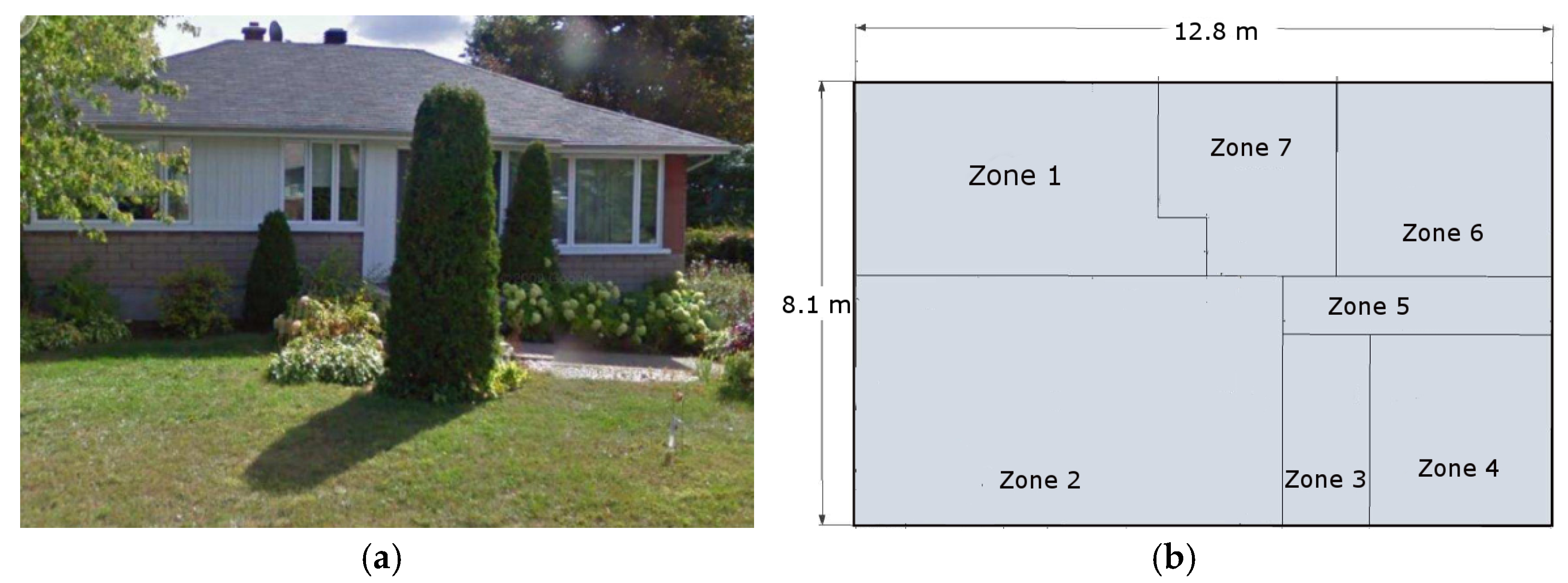
Simulations were performed on a reference residential building [21]. The modeled building was built in the 1960s, and has a basement and a first floor, Figure 3. The EHF was implemented in the first floor, which is then connected to the ground (the basement was removed to simulate a one-story building for this study). The building is located in Montreal (QC, Canada), with outdoor temperatures varying between −27 °C and 1 °C in January.

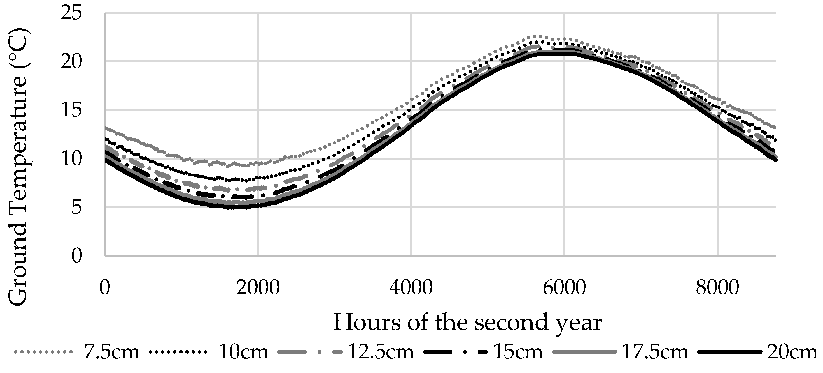
The ground temperature below the EHF was calculated using the Type 1244 [25]. To be able to consider the ground temperature without any initial condition, some simulations were performed for a two-year time period. Thus, results from the second year only were implemented. These results, as function of the insulation thickness on the bottom, are presented in Figure 4. They show that the floor heating system heats the surrounding ground, particularly when the insulation thickness is low.

The convective heat transfer coefficient of the floor heating system was set equal to 3.05 W/m² ·K [26]. To calculate the radiative heat transfer, TRNSYS considers the emissivity of surfaces (0.9 in this study). Then, the radiative heat transfer is distributed proportionally at the surfaces. The floor assembly of the EHF consists of five layers (Figure 5).

Table 2. Floor layers thermos-physical properties.

Themos-Physical Properties	Conductivity (W/m·K)	Specific Heat (kJ/kg·K)	Density (kg/m3)
Concrete	2.25	0.99	2200
Insulation (XPS)	0.04	1.5	35
Floor Covering (plywood)	0.164	1.63	670

gives the thermo-physical properties of the materials. All the following simulations were carried out throughout the month of January.

2.2. Study of the Performance of an EHF

The residential building was modeled in TRNSYS to study the performance of the EHF system for load management in a cold climate with a time step of 5 min. The peak period is from 6:00 a.m. to 8:00 p.m. The EHF is heated from 8:00 p.m. to 6:00 a.m. at rate of 120 W/m², and the heater is turned off when the Floor Surface Temperature (FST) exceeds 28 °C or when the operative temperature is higher than 24 °C.

2.2.1. Parametric Study

Extensive simulations were carried out to study the impact of the floor assembly on the EHF system performance, see Figure 5. In this study, the impact of the insulation thickness on the bottom, the concrete thickness below the wires, the concrete thickness above the wires, and the insulation thickness on the top (between the concrete and the floor covering) on the performance of the EHF are studied by modifying one thickness at a time. For this last parametric study, the idea to add an insulation layer on the top of the concrete layer is to investigate the possibility to store more energy in allowing higher concrete temperatures. The simulation was done for the month of January. Results were compared with the reference case (Figure 5), and the simulation results were analyzed in terms of energy consumption, floor surface and room temperatures, as presented in

Table 3. Studied parameters for the parametric study.

Floor Surface Temperature (FST)	Max Tfloor_surf	Maximal FST, averaged for the month for all the rooms (°C)
	Daytime Tfloor_surf	Daytime when the FST is at its maximal each day, averaged for the month for all the rooms. For example, 7:00 a.m. means that the maximal FST appears generally at 7:00 a.m. every day and decreases after (hh:mm)
	Tfloor_surf at 8:00 p.m.	FST at the end of the peak period (8:00 p.m.), averaged for the month for all the rooms (°C)
Operative Temperature	Max Top	Maximal operative temperature, averaged for the month for all the rooms (°C)
	Daytime Top max	Daytime when the operative temperature is at its maximal each day, averaged for the month for all the rooms. For example, 11:00 a.m. means that the maximal operative temperature appears generally at 11:00 a.m. every day and decreases after (hh:mm)
	Daytime Top < 20 °C	Daytime when the operative temperature drops below 20°C each day. For example, 8:00 p.m. means that the operative temperature is above 20 °C until 8:00 p.m. and drops below 20°C after (hh:mm)
Energy consumption	E	Energy consumption of the EHF for all the rooms in kWh, averaged by day (kWh/day)

.

2.2.2. Thermal Comfort

The thermal comfort provided by the EHF is estimated using the predicted percentage of dissatisfied (PPD) and the predicted mean vote (PMV) indexes (EN ISO 7730 [27]). These are the outputs of TRNSYS simulation. A clothing factor of 1 clo, a metabolic rate of 1.1 met and a relative air velocity of 0.1 m/s are considered. Median, minimal, maximal and (10th–90th) percentile range of the PPD and PMV are evaluated for each zone of the building.

2.2.3. Adaptation of Indicators for Sensible Thermal Storages

A large variety of thermal storage systems are available for residential buildings [28]. However, it is not easy to compare them and evaluate the most efficient storage system due to the variety of building types, the weather, etc. Some indicators such as the charged shelf life have been used [29,30,31].

To be able to completely understand the advantages and shortcomings of each possibility, some indicators are presented. Although most of the definitions can be extended to daily sensible thermal storages, only EHFs are discussed in this paper. Indicators have to be calculated in terms of the average for at least one month of $N_d$ days. To compare results, they have to be calculated based on the same building. Results of the building with an EHF (Case 1—with storage) and of the same building heated by electric baseboards (Case 2—without storage) are used.

Energy Storage Density—ESD (kWh/m³)

The energy storage density identifies the storage system capacity, considering the properties of the storage material and the temperature difference between the minimal storage temperature and the maximal temperature of the storage material.

$$ESD=C_p\times ∆T\times \mathsf{\rho }$$

(1)

where C_p and ρ are the specific heat and density of storage media (see Table 1). For this study, the room temperature is considered as the minimal storage temperature (calculated from average operative temperatures for Case 2), and the maximal storage temperature is considered as the average temperature of the slab when the FST is at 28 °C(30.5 °C for Case 1).

Payback Period—$N_{PB}$ (Years)

The payback period shows the required number of years to have a financially profitable system.

$$N_{PB}= \frac{c_{in{i}_1}+c_{om\_1}-c_{om\_2} }{ CE{S}_2\times E_{tot-2_{year}}-CE{S}_1\times E_{tot-1_{year}}}$$

(2)

where:

$$CE{S}_1=\left({\displaystyle \sum }_{i=1}^{N_d}{c}_{e_{off}peak}\times E_{offpeak\_1}+ c_{e_{peak}}\times E_{peak\_1}\right)/E_{tot\_1}$$

(3)

$$CE{S}_2=\left({\displaystyle \sum }_{i=1}^{N_d}{c}_{e_{off}peak}\times E_{offpeak\_2}+c_{e_{peak}}\times E_{peak\_2}\right)/E_{tot\_2}$$

(4)

where

• $c_{in{i}_1}$ and $c_{om\_1}$ are respectively the initial cost and maintenance cost of the system with storage
• $c_{om\_2}$ is the maintenance cost of the system without storage
• $c_{e_{off}peak}$ and $c_{e_{peak}}$ are the energy prices during off-peak and peak, respectively,
• $E_{offpeak\_1}$ and $E_{offpeak\_2}$ are the consumption during off-peak periods per day respectively with storage system and without storage system
• $E_{peak\_1}$ and $E_{peak\_2}$ are the consumption during peak periods per day respectively with storage system and without storage system
• $E_{tot\_1}$ and $E_{tot\_2}$ are the total consumption for space heating for $N_d$ days respectively with storage system and without storage system, and
• $CE{S}_1$ and $CE{S}_2$ are the average energy price for $N_d$ days with storage system and without storage system, respectively.

Depending on the availability of the data and the goal of the study, some parameters may be considered differently:

• For the consumption of the heating system for one year without the storage system ($E_{tot-2_{year}}$), historical data may be used to define the consumption of the system without storage in the case of an existing building.
• In Equation (2), only the initial cost of the heating system associated with storage is considered. That means most of the installations are for retrofitted buildings. For a new building, the price difference between the price of the heating system with storage and the price of the heating system without storage may be considered.
• Energy costs during peak and off-peak periods may be the cost for customers or for the supplier, depending if the study is done on the potential savings for the customer or for the supplier.

In this study, the maintenance costs of the system with storage and without storage are considered equal. Moreover, in this study, the calculation of the ratio between peak and off-peak energy consumption has been done only for January, the critical period for space heating period. Finally, the reference building, with electric baseboards and with a set-point of 21 °C, had a total energy consumption of 81.7 kWh/day, with 55% of the consumption during the day.

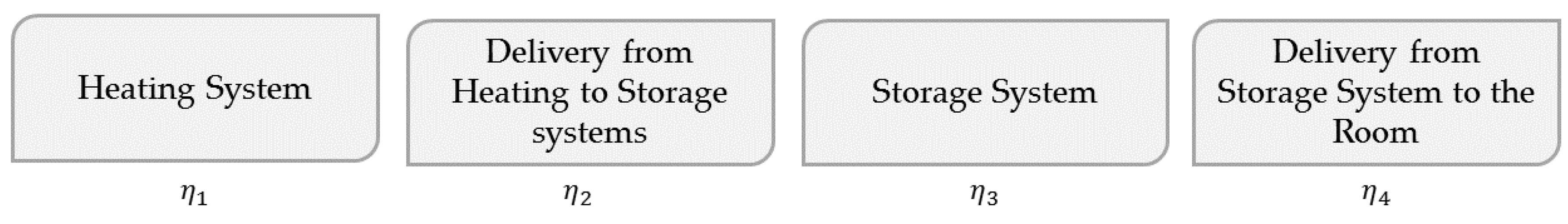
Energy Conversion Efficiency—η [-]

The energy conversion efficiency is one of the most important indicators: it is the ratio of the useful output (the building demand during the discharging time) of a system to the input (the required energy consumption during the charging time). The complexity of efficiency definition is to define what the input is. In particular, for a storage system coupled with a heating or cooling systems, two different efficiencies can be defined: the efficiency of the storage system itself, and the efficiency of the whole system, from the heating/cooling system to the delivery system including the storage system, see Figure 5.

Ma et al. [32] provides three definitions of the efficiency for a sensible thermal storage (hot water tank): the storage fraction, which represents the usable portion of the heat stored (with a tank for example, a portion of the fluid cannot be used); the first law efficiency, which defines the ratio of the actual energy discharged to the stored thermal energy, taking into account losses; and the second law efficiency is the exergy definition, taking losses and potential ineffectiveness of a part of the storage system into account.

The choice of a storage material also depends on the heating system type. For example, with a floor heating system embedded in concrete, the storage system is the concrete. However, the profitability of the whole system depends on the heating system (electric or hydronic, water heated by solar panels or electricity, etc.). Then, to be able to compare the energy conversion efficiency of various storage systems, the heating system type must also be considered. Efficiencies of each component of a heating system with a storage system are presented in Figure 6.

Therefore, with a simple control strategy, the energy conversion efficiency of a heating system with storage can be defined as:

$$\mathsf{\eta }=\frac{E_{deliveredtotheroom}}{E_{consumedbytheheatingsystem}}= {\mathsf{\eta }}_1\times {\mathsf{\eta }}_2\times {\mathsf{\eta }}_3\times {\mathsf{\eta }}_4$$

(5)

In this case study, ${\mathsf{\eta }}_1$ is set equal to 1 because 100% of the electric energy is converted to thermal energy. Then, 100% is stored in the concrete ${\mathsf{\eta }}_2$ = 1). The storage system has some losses to the ground, with

$${\mathsf{\eta }}_3= \frac{E_{deliveredtothestorage system}-Losstotheground}{E_{deliveredtothestorage system}}$$

Thermal energy loss to the ground is calculated for the month of January using the output QCOMO of TRNSYS considering losses during both charging and discharging periods. QCOMO gives the total energy losses [33]. The slab temperature at the end of the month is equal to the temperature at the beginning of the month: there is no accumulated energy. ${\mathsf{\eta }}_4$ is equal to 1 when 100% of the stored energy that is not lost to the ground is delivered to the room.

Charge/Discharge Ratio—CDR [-]

The charge/discharge ratio (CDR) is an important factor for load management. In the case of an EHF, because (heat production-storage-emissions) are in the same system, the CDR can be defined for the EHF by itself.

Depending on what is desired, for the same amount of stored energy, some storage energy systems are able to release a large amount of energy in a short period of time, while others release it during a longer period of time. To characterize this particularity, a charge/discharge ratio is proposed. This means, a system with a high CDR allows the shifting of short peak periods with high peaks while a lower CDR allows the shifting of longer peak period with lower peaks. For a night-control strategy, a low CDR is required.

CDR = CT/DT

(6)

Considering the maximal electrical power of the heating system ${\left(P_{max}\right)}_{Heatingsyst}\left(kW\right)$ and V the volume of the storage system, the charging time is considered as the duration (per day) needed to completely charge the system. It can be estimated as follows:

$$CT=\frac{ESD\times V\times {\mathsf{\eta }}_1\times {\mathsf{\eta }}_2}{{\left(P_{max}\right)}_{Heating syst}}$$

(7)

It is more complicated to define the discharging time. In fact, as a capacitor, the discharge power of a sensible thermal storage system decreases exponentially with the decrease of the temperature difference. The electrical network analogy is used to calculate the discharge time (DT). In this study, 90% is selected to characterize the discharge time:

$$DT=\ln \left(10\right)\times RC$$

(8)

where R and C are defined as:

$$\begin{gathered} R=1/h \\ C=C_p\times \mathsf{\rho }\times {\mathsf{\eta }}_3\times {\mathsf{\eta }}_4\times e \end{gathered}$$

(9)

where h is the total heat transfer coefficient. The value is defined as 11 W/m²·K [34,35,36].

3. Results

3.1. Parametric Study

3.1.1. Insulation on the Bottom

Table 4. Results of the parametric study: Impact of the lower layer Insulation thickness.

Thickness of Insulation on the Bottom (m)	FST			Operative Temperature			E (kWh/Day)
	Max Tfloor_surf (°C)	Daytime Tfloor_surf Max ($\mathit{h}\mathbf{:}\mathit{m}$)	Tfloor_surf at 8:00 pm (°C)	Max Top (°C)	Daytime Top Max ($\mathit{h}\mathbf{:}m$)	Daytime Top < 20 °C ($\mathit{h}\mathbf{:}\mathit{m}$)
0.075	28.02	6:33 am	23.64	23.08	10:52 am	10:25 pm	102.88
0.100 Reference case	28.16	6:19 am	23.85	23.22	10:39 am	10:50 pm	98.71
0.125	28.22	6:03 am	23.99	23.30	10:34 am	10:59 pm	95.78
0.150	28.28	6:01 am	24.09	23.36	10:28 am	11:09 pm	93.56
0.175	28.30	5:53 am	24.17	23.41	10:24 am	11:15 pm	91.86
0.200	28.33	5:48 am	24.24	23.44	10:25 am	11:20 pm	90.53

shows that the maximal FST, the FST at 8:00 p.m., and the maximal operative temperature increase as a function of the insulation thickness. With the increase of the insulation thickness, heat loss to the ground decreases: a higher proportion of the heat flux ends up in the room resulting in an increase in the maximal FST and the operative air temperature. For that same reason, the maximal FST and operative air temperature appear earlier, and the operative temperature stays above 20 °C for a longer period of time. Finally, the energy consumption decreases significantly as the insulation thickness increases. Hence, a thicker layer of insulation between the ground and the concrete layer is desirable for an EHF.

3.1.2. Concrete on the Bottom

Table 5. Results of the parametric study: Impact of the lower layer concrete thickness.

Thickness of Concrete on the Bottom (m)	FST			Operative Temperature			E (kWh/Day)
	Max Tfloor_surf (°C)	Daytime Tfloor_surf Max ($\mathit{h}\mathbf{:}\mathit{m}$)	Tfloor_surf at 8:00 pm (°C)	Max Top (°C)	Daytime Top Max ($\mathit{h}\mathbf{:}\mathit{m}$)	Daytime Top < 22 °C ($\mathit{h}\mathbf{:}\mathit{m}$)
0.02 Reference Case	28.16	6:19 am	23.85	23.22	10:39 am	150 pm	98.71
0.04	28.23	7:15 am	24.75	23.50	11:39 am	11:30 pm	100.21
0.06	28.21	7:57 am	25.34	23.65	11:59 am	11:41 pm	101.17
0.08	28.15	8:26 am	25.70	23.71	12:11 am	11:46 pm	101.79
0.10	28.04	8:29 am	25.88	23.69	12:13 am	11:47 pm	102.08
0.12	27.95	8:25 am	25.98	23.66	11:52 am	11:48 pm	102.04
0.14	27.89	8:19 am	26.04	23.64	11:43 am	11:49 pm	102.01

shows that several parameters (Daytime of the T_{floor_surf} max, FST-at-8:00 p.m., Daytime of operative temperature above 20 °C, the energy consumption and the maximal operative temperature) can be considered as constant between 8 and 14 cm of concrete on the bottom of the EHF (with a constant 10 cm of concrete on the top of the EHF). Thus, having a concrete thickness below the EHF higher than 8 cm (total concrete thickness of 18 cm) does not improve the performance of the thickness.

Table 5 also indicates that between concrete thickness of 2 and 8 cm on the bottom, the maximal FST decreases while the FST-at-8:00 p.m. increases, the maximal FST and operative temperature appear later, and the duration with a good TC is extended: the storage capacity has increased. Thus, between 2 and 8 cm of concrete on the bottom, one can observe a slight improvement of the performance of the system (for example, the period of time with an operative temperature staying above 20 °C is increased of more than one hour). This is due to an increase of the storage capacity of the system. Thus, one can conclude that a small increase of the concrete thickness increases the storage capacity, and thus provides the required TC for a longer period of time. However, from 8 cm, it appears that, with already 10 cm of concrete layer on the top of EHF, increasing the concrete thickness below the EHF does not impact the system performance.

3.1.3. Concrete on the Top

Further simulations were performed to investigate the impact of the thickness of the upper (screed) layer of concrete on the thermal behavior of the building.

Table 6. Results of the parametric study: Impact of the top layer concrete thickness.

Thickness of concrete on the top (m)	FST			Operative Temperature			E (kWh/Day)
	Max Tfloor_surf (°C)	Daytime Tfloor_surf max ($\mathit{h}\mathbf{:}\mathit{m}$)	Tfloor_surf at 8:00 pm (°C)	Max Top (°C)	Daytime Top max ($\mathit{h}\mathbf{:}\mathit{m}$)	Daytime Top < 20 °C ($\mathit{h}\mathbf{:}\mathit{m}$)
0.02	28.46	4:12 am	19.02	22.46	7:56 am	3:52 pm	90.54
0.04	28.21	4:37 am	20.82	22.67	8:54 am	6:28 pm	93.41
0.06	28.12	4:44 am	22.09	22.85	9:33 am	8:29 pm	95.49
0.08	28.13	5:31 am	23.05	23.02	10:13 am	10:01 pm	97.18
0.10 Reference Case	28.16	6:19 am	23.85	23.22	10:39 am	10:50 pm	98.71
0.12	28.21	7:04 am	24.58	23.43	11:25 am	11:21 pm	100.15
0.14	28.26	7:50 am	25.20	23.61	11:48 am	11:37 pm	101.79

shows that as the concrete thickness on the top increases, the maximal operative temperature and the FST-at-8:00 p.m. increase. Moreover, the maximal FST, the maximal operative temperature and the drop of the operative temperature above 20 °C appears significantly later. In fact, with the increase of the concrete thickness, a higher amount of energy is stored and released. Finally, the increase of the concrete thickness increases the energy consumption until provide enough energy to have an acceptable TC (operative temperature higher than 20 °C until the end of the peak period from 6 cm of concrete). In summary, the screed layer thickness has an important effect on the EHF performance. It allows more energy to be stored thus provides a longer period of acceptable TC for the occupants.

To compare the two concrete layers, the case with 4 cm of concrete on the bottom (and 10 cm on the top) and the case with 12 cm of concrete on the top (and 2 cm of concrete on the bottom) are compared. The results are really close. Thus, the concrete thickness has a significant impact on the performance, not the position of the concrete regarding the EHF.

3.1.4. Insulation on the Top

In this part, a thin layer of insulation on the top (between the concrete and the floor covering) is considered to study the possibility to increase the concrete temperature.

Table 7. Results of the parametric study: Impact of the top layer insulation thickness.

Thickness of Insulation on the Top (m)	FST			Operative Temperature			E (kWh/day)
	Max Tfloor_surf (°C)	Daytime Tfloor_surf Max ($\mathit{h}\mathbf{:}\mathit{m}$)	Tfloor_surf at 8:00 pm (°C)	Max Top (°C)	Daytime Top Max ($\mathit{h}\mathbf{:}\mathit{m}$)	Daytime Top < 20 °C ($\mathit{h}\mathbf{:}\mathit{m}$)
0 Reference Case	28.16	6:19 am	23.85	23.22	10:39 am	10:50 pm	98.71
0.01	27.39	9:31 am	25.14	23.13	12:14 am	10:35 pm	107.60
0.02	26.07	11:01 am	24.39	22.15	12:03 am	10:40 pm	110.41
0.03	25.06	11:11 am	23.61	21.31	12:17 am	6:53 pm	113.39
0.04	23.73	11:46 am	22.46	20.17	12:01 am	8:07 pm	116.20
0.05	22.31	12:09 am	21.13	18.93	11:59 am	-	117.91

shows a decreasing of the maximal FST, the maximal operative temperature, and the duration over the day with an operative temperature above 20 °C when the thickness of the insulation is increased. In addition, the electrical energy consumption increases with the insulation thickness. This is mainly because as insulation thickness on the top increases, the proportion of heat loss to the ground increases. Thus, the occupants’ TC decreases significantly. Table 7 also shows that the electrical energy consumption does not increase between 4 and 5 cm, because the EHF has been already 100% charged during the night.

3.2. Thermal Comfort

3.2.1. Total Night-Control Strategy

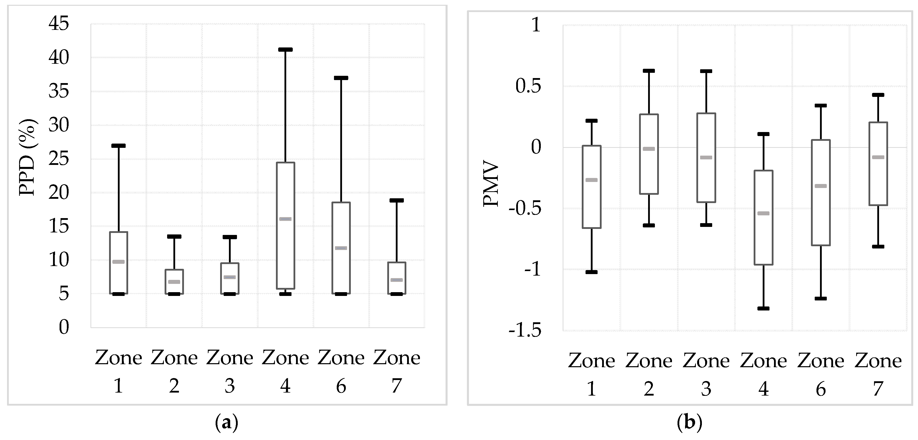
Concerning the thermal comfort, the PPD and PMV are studied for the reference case (Figure 5). To visualize the results, Figure 7 shows the minimal and maximal (black limits), the median (in grey) and the 10th and 90th percentile (the box) for PMV and PPD.

Figure 7a, showing the PPD results, allows to observe important differences between zones. The zone facing south (Zone 2) and zones with low thermal losses keep an acceptable thermal comfort (90th percentile below 10%). However, zones 1, 4 and 6 have some comfort issues. To understand these results, PMV are presented in Figure 7b. Results show that the dissatisfaction in zone 1, 4 and 6 is due to an underheating of these zones (PMV almost always negative, and sometimes below −1). Moreover, in the zones facing south (2 and 3), a slight over-heating may be observed.

Thus, the thermal comfort is not acceptable in all zones with a night-running strategy. Thus, to assure the thermal comfort of occupants in these zones, allowing the EHF to heat during the day in these zones is obligatory.

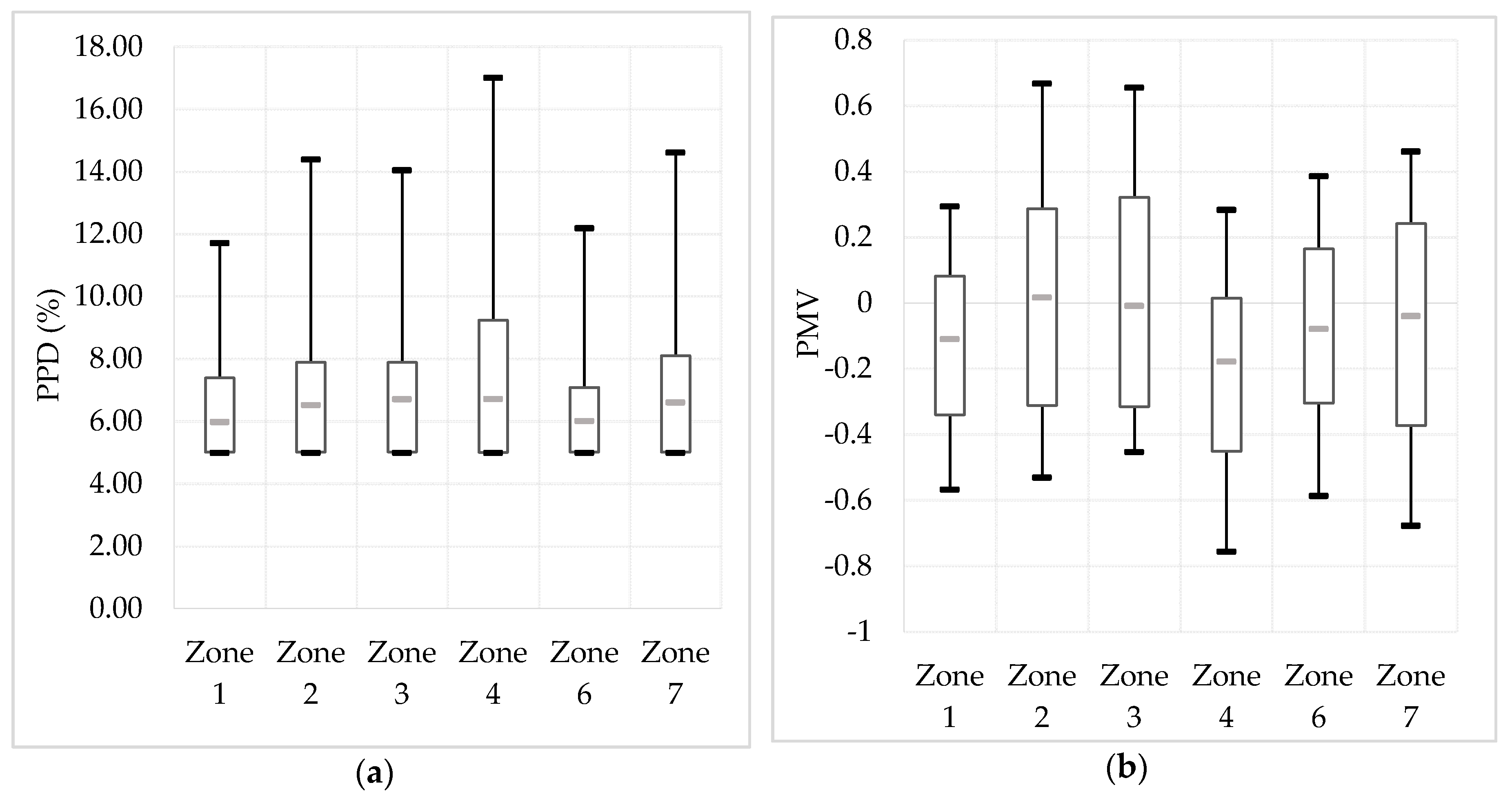
3.2.2. Partial Night-Control Strategy

The system is now allowed to heat zones 1, 4 and 6 when their operative temperature is below 23 °C between 9:30 a.m. and 4:00 p.m. Results in terms of thermal comfort are presented in Figure 8.

Figure 8 shows that the 90th percentile of the PPD stays below 10% for all the zones. Moreover, the (10th–90th) percentiles range of the PMV stay between −0.5 and 0.5 in all the zones. Thus, it can be concluded that the thermal comfort of this system is acceptable for occupants.

The possibility of heating between 9:30 a.m. and 4:00 p.m. in three zones lead to 84% of the total energy consumption during the night and 16% between 9:30 a.m. and 4:00 p.m. (with a total energy consumption per day of 99.68 kWh). This scenario will be used later in this paper.

3.3. Indicators

3.3.1. Comparison of the Two Systems

Indicators previously defined are calculated for the reference case of the EHF. However, these indicators are useful to compare systems with each other.

As discussed, the bottom insulation thickness is an important factor for a floor heating system and can result in significant energy savings. However, it can be difficult to decide to increase this layer thickness due to the initial cost. Then, a system with a thicker insulation layer in comparison with the reference case is studied. Two scenarios are considered: one with a low insulation thickness (10 cm of XPS − R = 2.5 m²·K/W—Reference case) and the other with a high insulation thickness (20 cm of XPS − 5 m²·K/W).

Table 8. Considered parameters to calculate the indicators.

Parameters	Unit	Value
Concrete price (per m2 of surface and cm of thickness)	$/m2/cm	2.1
XPS price (per m2 of surface and cm of thickness)	$/m2/cm	2.5
Electrically Heated Floor System	$/m2	65
Cost of the electricity (same during off-peak and peak periods)	$/kWh	0.10

gives the required inputs for this evaluation. The peak and off-peak electricity prices are considered equal.

Results are presented in

Table 9. Indicators for the EHF system for two different insulation thicknesses.

Indicators	Unit	Reference Case	R = 5 m2·K/W
ESD	kWh/m3	5.75	5.75
Efficiency	-	0.80	0.89
CDR	-	0.48	0.43

. The ESD is the same for the two configurations since the thickness of the concrete remains the same. Moreover, since the increase of the insulation thickness reduces losses to the ground, the energy conversion efficiency increases and the CDR decreases, this means the discharging time increases. One can observe that both are low: the discharging time of an EHF may be two times longer than the charging time, what is suitable for a night-running EHF.

However, it is not possible to calculate a payback period. In fact, electricity prices for off-peak and peak periods have been considered equal (as it is in Quebec). Thus, because an EHF consumes more energy than electric baseboards, the system will never be financially profitable without a time-of-use rate is not financially profitable. It is necessary to conduct an economic analysis to study the conditions needed to have a profitable system.

3.3.2. Economic Analysis

Considering the economic point of view, an EHF suffers from two issues: the initial cost of an EHF is important, and it can increase the electrical energy consumption due to heat losses to the ground. In addition to studying the thermal comfort or the peak shaving of the system, an economic feasibility analysis is required both from the point of view of the customer or the supplier.

The focus of this study is on the load management due to an EHF. Then, from an economical point of view, the customer and the supplier may both benefit from the peak shifting.

In fact, as it was discussed previously, from the customer point of view, a time-of-use tariff is available in many countries, differentiating peak periods (higher cost) and off-peak periods (lower cost). On the other hand, from the supplier point of view, peak periods lead to an increase of the electricity production cost. Then, the shift of a part of the consumption will provide financial savings for the supplier.

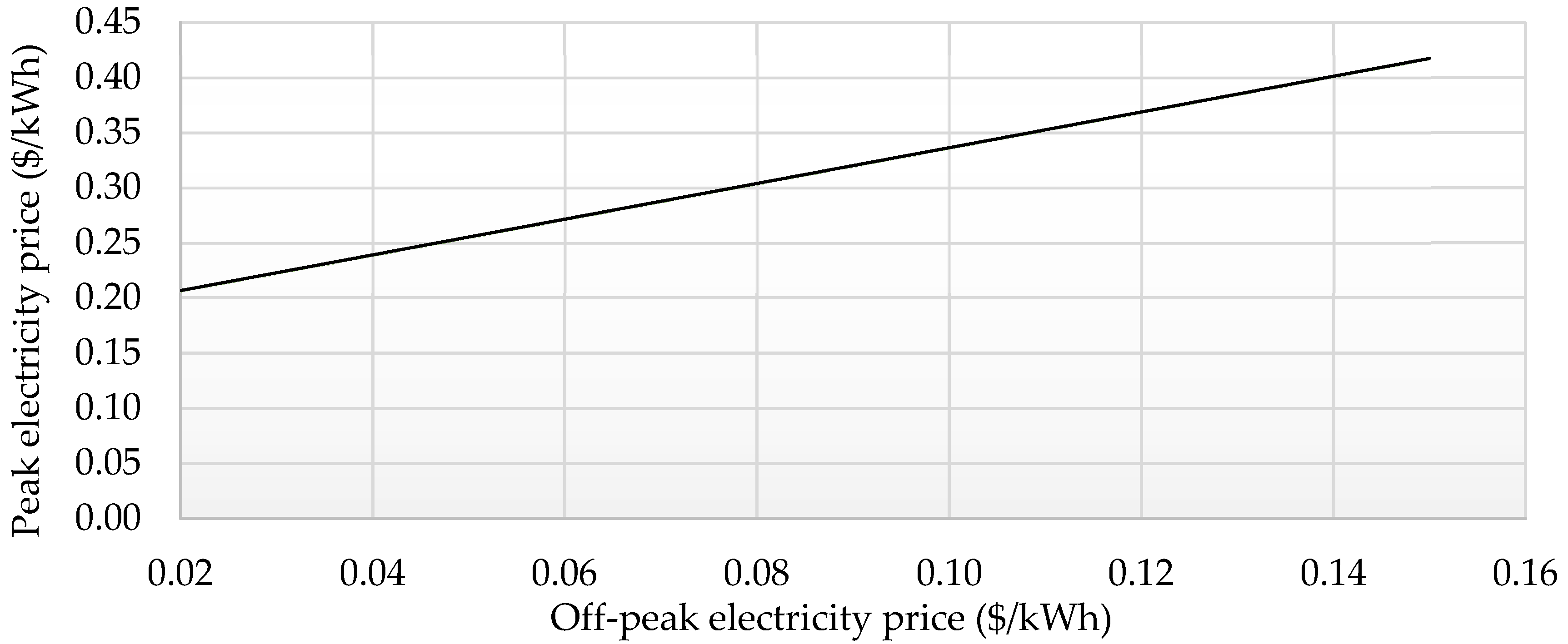
Due to the shift of the consumption from peak periods to off-peak periods, the greatest the difference between off-peak and peak electricity prices is, the more financially profitable the EHF is. To study the financial profitability of the EHF, the peak electricity price is calculated as a function of the off-peak electricity price from Equations (2) to (4) to have a payback amount per year equal to 0 (Equation (10)). A payback period of 15 years is considered.

$$c_{e_{peak}}=\frac{N_{PB}*c_{e_{off}peak}*({\displaystyle {\sum }_{i=1}^{N_d}\frac{E_{offpea{k}_2}}{E_{to{t}_2}}*E_{tot-2_{year}}-{\displaystyle {\sum }_{i=1}^{N_d}\frac{E_{offpea{k}_1}}{E_{to{t}_1}}*E_{tot-1_{year}}}})-c_{in{i}_1}-c_{om\_1}}{N_{PB}*({\displaystyle {\sum }_{i=1}^{N_d}\frac{E_{pea{k}_1}}{E_{to{t}_1}}*E_{tot-1_{year}}-{\displaystyle {\sum }_{i=1}^{N_d}\frac{E_{pea{k}_2}}{E_{to{t}_2}}*E_{tot-2_{year}}}})}$$

(10)

In the case of the studied EHF, Equation (11) is obtained, and results are presented in Figure 9.

$$c_{e_{peak}}= 1.6211\times c_{e_{off}peak}+0.1742$$

(11)

Equation (10) can be considered from the customer point of view in considering the electricity tariff, or for the supplier considering production costs. One can observe that the required peak/off-peak electricity price ratio decreases when the off-peak price increases. In fact, when the electricity price is higher, savings will be higher for the same peak/off-peak electricity ratio: a lower ratio between peak and off-peak electricity prices is required to have a profitable system.

Because of the initial cost of the system, the difference has to be important. However, in countries with high electricity price, the required ratio may be less than 3. For example, for residential buildings, the average electricity price in Massachusetts (US) is higher than 0.20 $/kWh. Thus, proposing an off-peak electricity price of 0.15 $/kWh and a peak electricity price of 0.42 $/kWh will allow to decrease at the same time bills of customers and peak period consumption for the supplier.

4. Discussion

The thermal comfort study showed that a complete night-control strategy was not possible in half of the zones (depending on the amount of external walls and their orientation). Thus, it was proven that an acceptable thermal comfort was achieved with only 16% of the energy consumption during the day (only between 9:30 a.m. and 4:00 p.m.). However, results show an overheating of some zones at some times during the day. In fact, the stored energy amount is not always required, involving overheating, especially in the zones facing the south. Then, using a different control strategy, which takes into consideration the amount of energy required for the next day in conjunction with the weather prediction, is required to improve the thermal comfort. Moreover, it is important to notice that, if the used building is representative of the dwellings in Quebec, results are situational to the example. Studies on different types of buildings are required draw conclusions about the feasibility of a night-control strategy for an EHF in cold climate.

Especially for the EHF, the payback period is an important indicator. Even if an EHF may have some financial issue (considering the initial cost and the increase of the consumption) it shows that the system may be financially profitable for both customer and supplier thanks to the shift in consumption. The economic viability depends on the off-peak electricity price/cost and the difference between it and the peak electricity price/cost. It is important to notice that this definition gives a conservative result of the real payback amount, since the simulation was only done during the month of January, one of the months with the highest heating loads. Then, for milder months, because the required energy is lower, a higher percentage of this amount may be stored in comparison to January. If a higher precision is required, instead of analyzing one month to determine the amount of energy consumed respectively during peak and off-peak periods, the analysis can be carried out for the entire year. Moreover, in this study, the cost of a system without storage is not considered, giving a conservative result of the real payback period. However, the maintenance cost of the system is ignored.

5. Conclusions

This paper investigates the performance in using an EHF to shift electrical loads from peak periods to off-peak periods in a cold climate. To perform the simulations, a method to implement an EHF in TRNSYS is developed and validated. Then, an EHF is implemented in a typical residential house, without a basement. Parametric studies were performed, thermal comfort was studied and indicators were defined to investigate the effect of the floor assembly on the EHF performance.

Results of the parametric study show that the insulation layer on the bottom of the floor assembly decreases heat loss to the ground, and may allow reducing the concrete layer thickness with the same TC. For the concrete layers, whether the concrete is below or above the wires, a significant impact on the system performance was evaluated, allowing to store energy and to keep an acceptable TC during the day when the heating system is off. A total concrete thickness thicker than 18 cm will not improve the performance of the system. Finally, having an insulation thickness on the top of the assembly stops the heat transfer to the room, thus increases heat loss to the ground.

Results show that the night-running EHF provides acceptable thermal comfort in half of zones. Finally, the thermal comfort was satisfied in all zones with 84% of the consumption during the night and without any consumption during early morning and evening. Nevertheless, slight overheating in some zones may appear. To solve this issue, a control taking into consideration weather prediction has to be studied.

Finally, four indicators were proposed to provide the required information for a heating system with a sensible thermal energy storage system. Moreover, concerning the application on the EHF, results show that an EHF is financially profitable if the peak/off-peak price ratio is high enough.

References

- Hydro-Quebec. Consommation Hivernale de L’electricite. Available online: http://www.hydroquebec.com/residentiel/mieux-consommer/comprendre-et-agir/consommation-hivernale/ (accessed on 5 July 2016).
- Guerassimoff, G.; Maïzi, N. Smart Grids: Au-delà du Concept, Comment Rendre les Réseaux Plus Intelligents; Presses des Mines-Transvalor: Paris, France, 2013. [Google Scholar]
- Henze, G.P.; Felsmann, C.; Knabe, G. Evaluation of optimal control for active and passive building thermal storage. Int. J. Therm. Sci. 2004, 43, 173–183. [Google Scholar] [CrossRef]
- Oldewurtel, F.; Ulbig, A.; Parisio, A.; Andersson, G.; Morari, M. Reducing peak electricity demand in building climate control using real-time pricing and model predictive control. In Proceedings of the 49th IEEE Conference on Decision and Control, Atlanta, GA, USA, 15–17 December 2010; pp. 1927–1932.
- Atikol, U. A simple peak shifting DSM (demand-side management) strategy for residential water heaters. Energy 2013, 62, 435–440. [Google Scholar] [CrossRef]
- Bastani, A.; Haghighat, F. Expanding Heisler chart to characterize heat transfer phenomena in a building envelope integrated with phase change materials. Energy Build. 2015, 16, 164–174. [Google Scholar] [CrossRef]
- Bastani, A.; Haghighat, F.; Kozinski, J. Designing building envelope with PCM wallboards: Design tool development. Renew. Sustain. Energy Rev. 2014, 31, 554–562. [Google Scholar] [CrossRef]
- El-Sawi, A.; Haghighat, F.; Akbari, H. Assessing long-term performance of centralized thermal energy storage system. Appl. Therm. Eng. 2014, 62, 313–321. [Google Scholar] [CrossRef]
- Nkwetta, D.N.; Vouillamoz, P.-E.; Haghighat, F.; El-Mankibi, M.; Moreau, A.; Daoud, A. Impact of phase change materials types and positioning on hot water tank thermal performance: Using measured water demand profile. Appl. Therm. Eng. 2014, 67, 460–468. [Google Scholar] [CrossRef]
- Nkwetta, D.N.; Haghighat, F. Thermal energy storage with phase change material—A state-of-the art review. Sustain. Cities Soc. 2013, 10, 87–100. [Google Scholar] [CrossRef]
- ASHRAE. ASHRAE Standard 55–2013: Thermal Environmental Conditions for Human Occupancy; ASHRAE: Atlanta, GA, USA, 2013. [Google Scholar]
- Ghali, K. Economic viability of under floor heating system: A case study in beirut climate. In Proceedings of the International Conference on Renewable Energies & Power Quality, Sevilla, Spain, 28–30 March 2007.
- Kattan, P.; Ghali, K.; Al-Hindi, M. Modeling of under-floor heating systems: A compromise between accuracy and complexity. HVAC R Res. 2012, 18, 468–480. [Google Scholar]
- Li, J.; Xue, P.; He, H.; Ding, W.; Han, J. Preparation and application effects of a novel form-stable phase change material as the thermal storage layer of an electric floor heating system. Energy Build. 2009, 41, 871–880. [Google Scholar] [CrossRef]
- Lin, K.; Zhang, Y.; Xu, X.; Di, H. Experimental study of under-floor electric heating system with shape-stabilized PCM plates. Fuel Energy Abstr. 2005, 46, 335. [Google Scholar] [CrossRef]
- Cheng, W.; Xie, B.; Zhang, R.; Xu, Z.; Xia, Y. Effect of thermal conductivities of shape stabilized PCM on under-floor heating system. Appl. Energy 2015, 144, 10–18. [Google Scholar] [CrossRef]
- Weitzmann, P.; Kragh, J.; Roots, P.; Svendsen, S. Modelling floor heating systems using a validated two-dimensional ground-coupled numerical model. Build. Environ. 2005, 40, 153–163. [Google Scholar] [CrossRef]
- Cvetkovic, D.; Bojic, M. Optimization of thermal insulation of a house heated by using radiant panels. Energy Build. 2014, 85, 329–336. [Google Scholar] [CrossRef]
- Wang, D.; Liu, Y.; Wang, Y.; Liu, J. Numerical and experimental analysis of the floor heat storage and release during an intermittent in-slab floor heating process. Appl. Therm. Eng. 2014, 62, 398–406. [Google Scholar] [CrossRef]
- A TRaNsient Systems Simulation Program. Available online: http://www.trnsys.com (accessed on 3 April 2015).
- Aongya, S. Contrôle du Chauffage Pour la Gestion de la Demande Résidentielle—Rapport Technique sur la Création d’ un Modèle Résidentiel Fonctionnel; Hydro-Quebec: Shawinigan, QC, Canada, 2010. [Google Scholar]
- Bastani, A.; Haghighat, F.; Manzano, C.J. Investigating the effect of control strategy on the shift of energy consumption in a building integrated with PCM Wallboard. Energy Procedia 2015, 78, 2280–2285. [Google Scholar] [CrossRef]
- ASHRAE. ASHRAE Guideline 14-2014, Measurement of Energy and Demand Savings; ASHRAE: Atlanta, GA, USA, 2014. [Google Scholar]
- Olsthoorn, D.; Haghighat, F. Modelling of electrically activated thermal mass. In CLIMA 2016; 12th REHVA World Congress: Aalborg, Denmark, 2016. [Google Scholar]
- TESS Component Libraries – General Descriptions. Available online: http://trnsys.con/tess-libraries/TESSLibs17_General_Descriptions.pdf (accessed on 6 January 2016).
- Cholewa, T.; Rosiński, M.; Spik, Z.; Dudzińska, M.R.; Siuta-Olcha, A. On the heat transfer coefficients between heated/cooled radiant floor and room. Energy Build. 2013, 66, 599–606. [Google Scholar] [CrossRef]
- International Organization for Standardization. ISO 7730: Moderate Thermal Environments—Determination of the PMV and PPD Indices and Specification of the Conditions for Thermal Comfort; International Organisation for Standardization: Geneva, Switzerland, 1994. [Google Scholar]
- Dincer, I.; Rosen, M. Thermal Energy Storage: Systems and Applications; John Wiley & Sons: Chichester, England, 2002. [Google Scholar]
- Wilbur, L.C. Handbook of Energy Systems Engineering—Production and Utilization; Wiley: New York, USA, 1985. [Google Scholar]
- Hassenzahl, W. Mechanical, Thermal and Chemical Storage of Energy; Hutchinson Ross Pub. Co.: Stroudsburg, PA, USA, 1981. [Google Scholar]
- Ibrahim, H.; Ilinca, A.; Perron, J. Energy storage systems—Characteristics and comparison. Renew. Sustain. Energy Rev. 2008, 12, 1221–1250. [Google Scholar] [CrossRef]
- Ma, Z.; Glatzmaier, G.; Turchi, C.; Wagner, M. Thermal energy storage performance metrics and use in thermal energy storage design. In Proceedings of the ASME 2012 6th International Conference on Energy Sustainability collocated with 10th International Conference on Fuel Cell Science, Engineering and Technology Conference, San Diego, CA, USA, 23–26 July 2012.
- TRNSYS 17 - Multizone Building modeling with Type56 and TRNBuild. Version 16. Available online: http://web.mit.edu/parmstr/Public/Documentation/06-MultizoneBuilding.pdf (accessed on 5 April 2015).
- Babiak, J.; Olesen, B.W.; Petras, D.; Federation of European Heating and Air-conditioning Associations. Low Temperature Heating and High Temperature Cooling : Embedded Water Based Surface Heating and Cooling Systems; REHVA, Federation of European Heating and Air-conditioning Associations: Brussels, Belgium, 2009. [Google Scholar]
- Rhee, K.-N.; Kim, K.W. A 50 years review of basic and applied research in radiant heating and cooling systems for the built environment. Build. Environ. 2015, 91, 166–190. [Google Scholar] [CrossRef]
- Olesen, B.W. Radiant floor heating in theory and practice. ASHRAE J. 2002, 44, 19–26. [Google Scholar]
© 2016 by the authors; licensee MDPI, Basel, Switzerland. This article is an open access article distributed under the terms and conditions of the Creative Commons Attribution (CC-BY) license (http://creativecommons.org/licenses/by/4.0/).