3D Ear Normalization and Recognition Based on Local Surface Variation

Abstract

Most existing ICP (Iterative Closet Point)-based 3D ear recognition approaches resort to the coarse-to-fine ICP algorithms to match 3D ear models. With such an approach, the gallery-probe pairs are coarsely aligned based on a few local feature points and then finely matched using the original ear point cloud. However, such an approach ignores the fact that not all the points in the coarsely segmented ear data make positive contributions to recognition. As such, the coarsely segmented ear data which contains a lot of redundant and noisy data could lead to a mismatch in the recognition scenario. Additionally, the fine ICP matching can easily trap in local minima without the constraint of local features. In this paper, an efficient and fully automatic 3D ear recognition system is proposed to address these issues. The system describes the 3D ear surface with a local feature—the Local Surface Variation (LSV), which is responsive to the concave and convex areas of the surface. Instead of being used to extract discrete key points, the LSV descriptor is utilized to eliminate redundancy flat non-ear data and get normalized and refined ear data. At the stage of recognition, only one-step modified iterative closest points using local surface variation (ICP-LSV) algorithm is proposed, which provides additional local feature information to the procedure of ear recognition to enhance both the matching accuracy and computational efficiency. On an Inter^®Xeon^®W3550, 3.07 GHz work station (DELL T3500, Beijing, China), the authors were able to extract features from a probe ear in 2.32 s match the ear with a gallery ear in 0.10 s using the method outlined in this paper. The proposed algorithm achieves rank-one recognition rate of 100% on the Chinese Academy of Sciences’ Institute of Automation 3D Face database (CASIA-3D FaceV1, CASIA, Beijing, China, 2004) and 98.55% with 2.3% equal error rate (EER) on the Collection J2 of University of Notre Dame Biometrics Database (UND-J2, University of Notre Dame, South Bend, IN, USA, between 2003 and 2005).

1. Introduction

Ear based human recognition technology is a novel research field in biometric identification. Compared with classical biometric identifiers such as fingerprints, faces, and irises, using an ear can has its distinctive advantages. An ear has a stable and rich structure that changes little with age and does not suffer from changes in facial expressions at the same time [1]. Moreover, the collection of ear images is deemed to be easy and non-intrusive. As such, ear biometrics has recently received some significant attention.

Researchers developed several approaches for ear recognition based on 2D ear images in the early years [2,3,4]. From those works, researchers found that the performances of 2D ear recognition methods were greatly affected by the pose variation and imaging condition. Compared with 2D ear images, the 3D ear data are relatively insensitive to illuminations and posture variation. Therefore, ear recognition methods utilizing 3D shape information have become a recent trend in research field [5,6,7,8,9,10].

Most existing 3D ear recognition approaches are based on the ICP (Iterative Closet Point) algorithm. Although ICP is thought to be the most accurate matching algorithm, it requires concise ear data and a good initial rigid transformation to ensure global convergence. Researchers have proposed several two-step ICP based matching techniques to register probe and gallery ear data [11,12]. In these methods, local surface descriptors were used to extract a set of key points on the ear surface which were only employed to estimate the initial rigid transformation between a gallery-probe pair. The fine matching was based on the entire ear region data. However, these methods were notably limited by the redundancy data and the computation load of a two-step ICP algorithm. The ear region data utilized in most of the existing methods were coarsely segmented from profile images, so there was a mass of non-ear data, such as flat face skin data and hair data. It is essential to refine and normalize the ear data since any extra data can lead to mismatching in the ICP algorithm.

In this work, instead of being used to extract key points, the local feature LSV (Local Surface Variation) is utilized to eliminate redundancy data from ear regions. The LSV is responsive to the concave and convex areas of the surface, so that the flat face skin data will be removed if the appropriate threshold value of LSV is selected. Furthermore, most of the hair data are removed and the ear pose is normalized via the proposed template matching methods. Therefore, the computation load of the ICP algorithm markedly drops down because the size of the normalized ear data is one third the size of the original data size.

With the ICP algorithm it is easy to fall into local minimum values without the constraint of local features. As such, the existing two-step ICP based matching techniques roughly align the gallery-probe pairs using key points during the coarse matching. However, the two-step ICP algorithm can be extremely time-consuming. To combine the local feature matching and global registration in the ICP algorithm, a modified ICP algorithm named ICP using Invariant Features (ICPIF) was proposed by Sharp [13]. Compared with traditional ICP, the corresponding points are selected according to a weighted linear combination of positional and feature distances in the ICPIF algorithm. It has been demonstrated that the ICPIF converges to the minimum distance with less iterations than the traditional ICP algorithm. Maximum and minimum principal curvatures are perhaps the most common invariant. However, it would increase the computation load to bring two feature distances into the iteration.

The proposed recognition procedure obtains a better performance than the traditional coarse-to-fine registration algorithm utilizing a one-step modified ICP algorithm. In this work, a modified ICPIF algorithm named ICP-LSV algorithm is proposed to provide only one LSV feature distance in order to avoid the local minimum and obtain fast and accurate convergence. As such, the initially rough alignment of gallery-probe pairs is not necessary in the proposed approach.

The rest of this paper is organized as follows: A review of related work and contributions are given in Section 2. Section 3 presents the technical approach of the ear recognition system. In Section 4, a series of experiments and comparisons are proposed to evaluate the performance of the system. Finally, Section 5 provides the conclusions.

2. Related Work and Contributions

Current 3D ear recognition approaches exploit 3D ear data or both 3D and co-register 2D ear data. This section discusses some well-known and recent 3D ear recognition methods and highlights the contributions of this paper.

2.1. Ear Detection and Segmentation

Detection and recognition are the two major components of a complete biometrics system. In this section, a summary of ear detection and segmentation approaches are provided. The existing ear detecting and ear region extracting approaches have been based on 2D or 3D profile images.

One of the 3D ear detection approaches was proposed by Chen and Bhanu, who combined 2D side face images and 3D profile range images to detect and extract human ears [11]. The edges were extracted to locate potential ear regions called regions-of-interest (ROIs). Then the reference 3D ear shape model, which was a set of discrete 3D vertices on the ear helix and the antihelix parts, was matched with individual ear images by following a modified ICP procedure. The ROI with the minimum Root Mean Square (RMS) error was considered to be the ear region. In a previous [14], Abdel-Mottaleb and Zhou put forward a 3D ear recognition approach in which the ear regions were segmented by locating the ridges and ravines on the profile images. However, it may be difficult to detect the ridges and ravines when the ear is partly occluded. In another study [15], Prakash and Gupta proposed a rotation and scale invariant ear detection technique from 3D profile images using graph inherent structural details of the ear in 3D range data. Maity et al. used an active contour algorithm and a tree structured graph to segment the ear region in [16]. Yan and Bowyer exploited an ear extracting approach based on ear pit detection and Active Contour Algorithm [17]. They found the ear pit using skin detection, curvature estimation, and surface segmentation and classification. Then an active contour algorithm was implemented to outline the ear region. All of the ear images on the University of Notre Dame (UND) database were correctly segmented using the combination of color and depth images in the active contour algorithm. However, since this method has to locate the nose tip and ear pit on the profile image, this algorithm may not be robust enough to pose variations or hair covering.

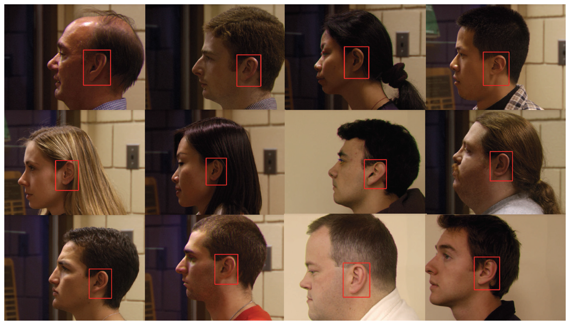
Researchers proposed some learning algorithms to detect ears under complex background from 2D images, where corresponding 3D ear data could thenbe extracted from the co-registered 3D images if necessary. Islam [12] detected ear regions on 2D profile images using a detector based on the AdaBoost algorithm. They argued that it was efficient and robust to noisy background and pose variation. Abaza et al. [18] modified the Adaboost algorithm and, in doing so, reduced the training time significantly. Shih et al. [19] presented a two-step ear detection system utilized arc-masking candidate extraction and AdaBoost polling verification. Firstly, the ear candidates were extracted by the arc-masking edge search algorithm; then the ear was located by rough AdaBoost polling verification. Yuan and Zhang [20] used the improved AdaBoost algorithm to detect ears under complex backgrounds. They sped up the detection procedure and reported a good detection rate on three test data sets.

It has been experimentally shown that the learning algorithms perform better than the algorithms based on ear edge detection or ear template matching on 2D images. However, shallow learning models such as Adaboost algorithm also lack robustness in realistic scenarios, which may contain occlusion, illumination variation, scaling, and rotation.

Recently, convolution neural network (CNN) has significantly pushed forward the development of image classification and object detection [21]. Girshick et al. [22] proposed a new framework of object detection called Regions with CNN features (R-CNN). The R-CNN approach achieved the best result on the Pattern Analysis, Statistical modelling and Computational Learning Visual Object Classes (PASCAL VOC 2010) Challenge. Then a modified network called Faster R-CNN was proposed by Ren et al. [23]. In this work, they introduced a Region Proposal Network (RPN) which shared the full-image convolutional features with the detection network. The detection system has a frame rate of 5 fps on Graphics Processing Unit (GPU), while achieving 70.4% mAP on PASCAL VOC 2012. Schemes based on Faster R-CNN have obtained impressive performance on object detection in images captured from real world situations. However, the application of ear detection using the Faster R-CNN algorithm has not been reported so far. In this work, ear images were coarsely extracted from 2D profile images utilizing an ear detection algorithm based on Faster R-CNN frameworks.

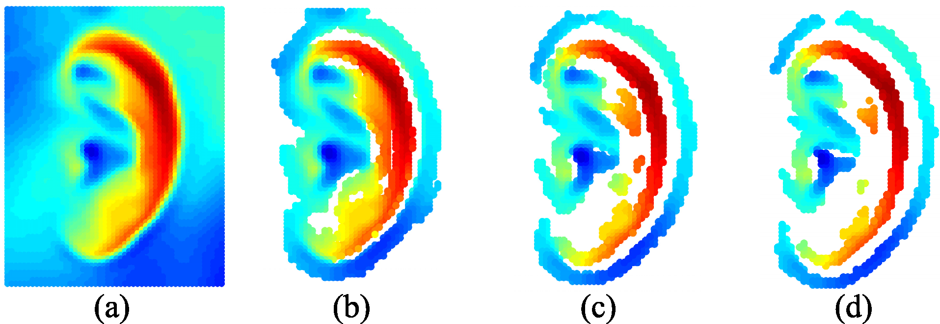
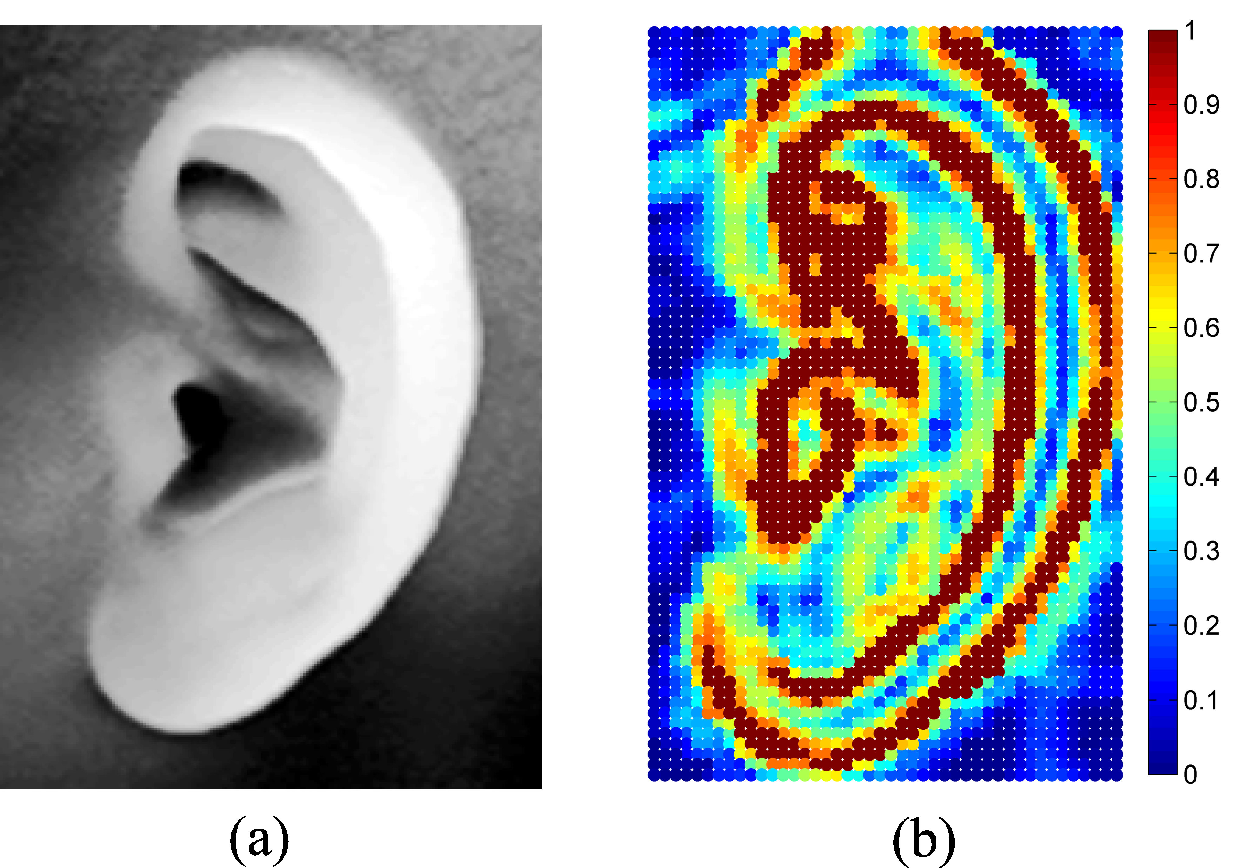
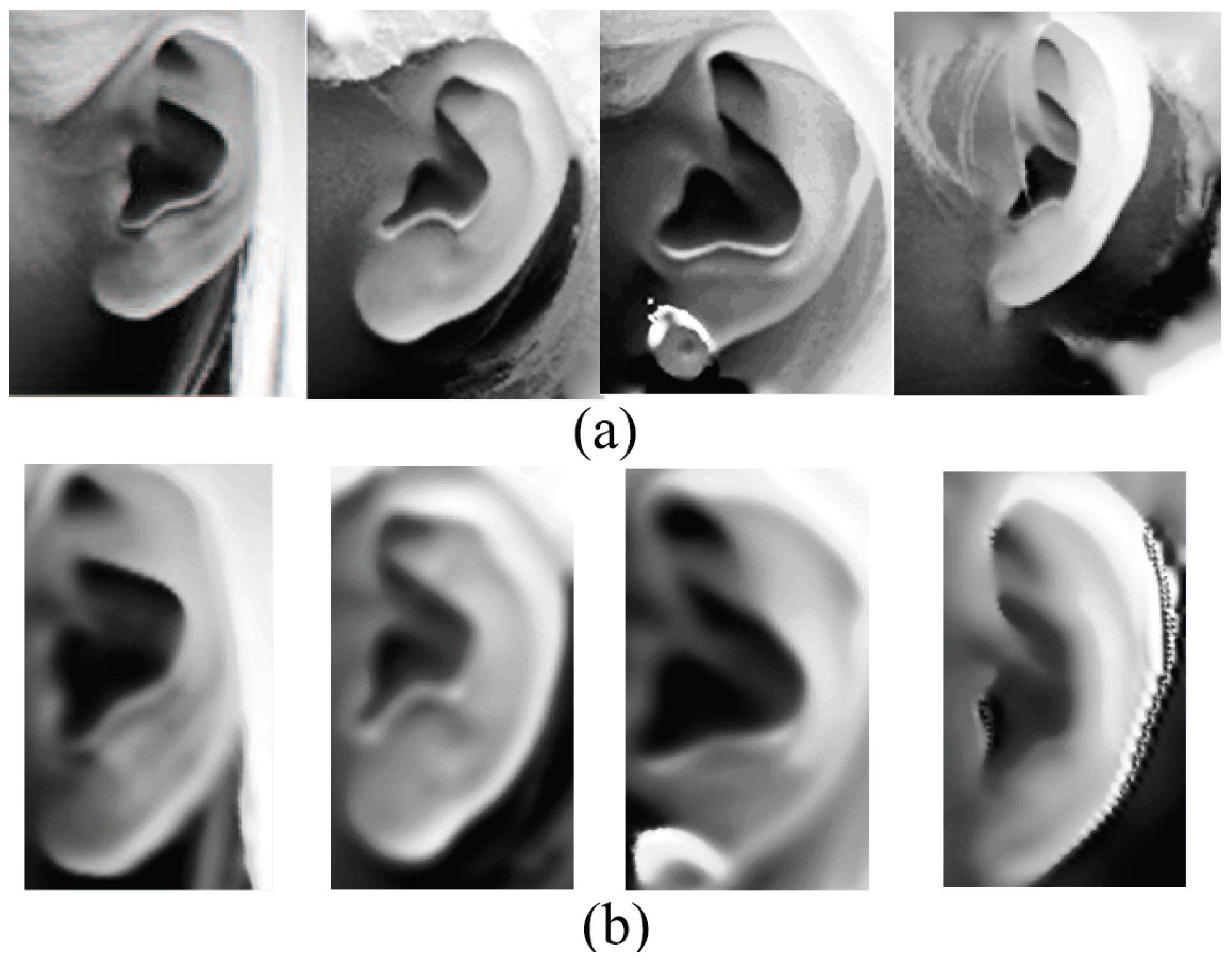
Ear data that has been extracted from profile views can be basically classified as pure data which are extracted along the ear edge and the rectangular ear region data. However, automatic extracting approaches of pure ear data based on 2D or 3D ear edge information are not robust to background noise or minor hair covering around the ear. As to ear region data, there is a lot of hair and face skin data in most cases. As we know, the hair data are considered to be a negative influence for an ear recognition system; in comparison with the ear, the flat face skin surface is not feature-rich. Researchers have experimentally demonstrated that the non-ear data barely have a positive contribution to recognition. After removing pure ear data manually from the ear region data, which are segmented by an AdaBoost detector, the rank-one recognition rate is only 27.2% [24].

2.2. 3D Ear Recognition

Existing 3D ear recognition approaches utilizing 3D point cloud or range images can be basically classified as local feature matching, ICP global registration, or a combination of both.

In a previous study [6], Sun et al. proposed a method to sort key points on point clouds for 3D ear shape matching and recognition. The Gaussian-weighted average of the mean curvature was utilized to select the salient key points. Then the angle between two feature vectors was used to calculate the similarity of two local features. Finally, the overall similarity of two ears was measured by the confidence weighted sum of all the measures. The approach achieved a rank-one recognition rate of 95.1% and an equal error rate (EER) of 4% on UND-J2 database. Zeng et al. proposed an ear recognition approach based on 3D key point matching in [25]. The 3D key points were detected using the shape index image and the scale space theory. Then they constructed 3D Center-Symmetric Local Binary Pattern (CS-LBP) features and used a coarse to fine strategy for 3D key point matching. The rank-one recognition rate on UND-J2 database was 96.39%.

The ICP algorithm is widely used to align 3D rigid models [26]. The algorithm obtains correspondences by looking for the closest points, and then minimizes the mean square distance between the pairs. Cadavid and Abdel-Mottaleb [27] proposed an approach based on ICP for 3D ear recognition using video sequences. They obtained 84% rank-one recognition rate on a database of 61 gallery and 25 probe images. Yan and Bower compared three ear based human recognition techniques in [28]. They explored the use of a Principal Component Analysis (PCA)-based approach on a range image representation of the 3D data, Hausdorff matching on edge images obtained from 3D ear images and an ICP approach on a point-cloud representation of the 3D data. They confirmed that ICP matching achieved the best performance. In their later work [17], Yan and Bower put forward an approach of 3D ear recognition according to the RMS registration error of the ICP algorithm. They used a k-d tree data structure in the search for closest points and limited the maximum number of iterations to reduce the time consumption. The system achieved a rank-one recognition rate of 97.8% on the UND database in the identification stage and an EER of 1.2% in the verification stage. However, only beginning with a translation vector which was estimated from the ear pit location, it took 5–8 s to match a pair of ears on a dual processor 2.8 Gigahertz (GHz) Inter^® Pentium Xeon system. Therefore, this indicated that an initial guess of the full 3D (translation and rotation) transformation is significant for an ICP-based algorithm.

Recently, the coarse-to-fine ICP based 3D ear recognition algorithm which combines local feature extraction and ICP global registration has drawn extensive attention. The gallery-probe pairs are coarsely aligned based on the local information extracted from the feature correspondences in order to get a relatively accurate initial transformation, and then are finely matched via the ICP global registration.

Chen and Bhanu detected and aligned the helix of the gallery-probe pairs to get the initial rigid transformation in [29]. Then the ICP algorithm iteratively refined the transformation to bring model ears and test ears into the best alignment. The recognition rate on a database of 30 subjects was 93.3%. In a previous study [11], Chen and Bhanu created the ear helix/antihelix representation and the local surface patch (LSP) representation, which were employed to estimate the initial transformation for a modified ICP algorithm separately. They obtained 96.03% and 96.36% recognition rates, respectively, on the Collection F of the UND database. Due to the high dimensionality of LSP feature representation, in their later approach [30], an embedding algorithm was employed to map the feature vectors to a low-dimensional space. The similarities for all model-test pairs were computed using the LSP features and ranked using SVM to generate a short list of candidate models for verification. The verification was performed by aligning a model with the test object via the ICP algorithm. On the UND Collection F, the rank-one recognition rate was 96.7%, and EER was 1.8%.

In a study by Islam et al. [31], a coarse-to-fine hierarchical technique was used where the ICP algorithm was first applied on low and then on high resolution meshes of 3D ear data. The rank-one recognition rates of 93% and 93.98% were achieved respectively on UND Biometrics Database A and Database B. In a later approach [12], Islam represented the 3D ear data with local 3D features (L3DF) to extract a set of key points for L3DF-based initial alignment, then the fine recognition result was obtained through the ICP algorithm. The system provided an identification rate of 93.5% on the UND-J database. Nevertheless, extraction of L3DF was relatively complex, so that the extraction time for a single ear was 22.2 s on an Inter^® Core^TM2 Quad 9550, 2.83 Gigahertz (GHz) machine.

Prakash and Gupta proposed a two-step matching technique which makes use of 3D and co-registered 2D ear images [32]. They extracted a set of local 2D features points using the Speed Up Robust Feature (SURF) descriptor. Then the co-registered salient 3D data points were used to coarsely align 3D ear points. The final matching was performed by integration of Generalized Procrustes Analysis (GPA) with ICP (GPA-ICP). The technique achieved a verification accuracy of 98.30% with an EER of 1.8% on the UND-J2 database. The key points were extracted from the 2D ear images—compared with 3D local descriptors, the SURF descriptor may not be robust to pose and illumination variations.

The schemes based on local feature matching and ICP global registration both have advantages and disadvantages for ear recognition. The matching method using local surface descriptors can represent free-form surfaces effectively, but it may cause mismatching within similar key points without global constraint. Although the ICP-based algorithm obtains high accuracy regarding the registering of 3D rigid models, it may be trapped in local minimum without an accurate initial rigid transformation. It is clear that the combination of local feature matching and ICP global registration in 3D ear recognition is effective. However, in the existing two-step alignment methods, the local feature points are extracted to refine the initial alignment, and then the results of matching are based on the ICP procedure using the original ear data. It treats all the points equally, regardless of how much useful information the point represents. However, it ignores the fact that not all the points in the coarsely segmented ear data make positive contributions to recognition. Since the local features can distinguish the useful data points from useless data, we do not have to utilize the original data to make the final decision according to the ICP-based matching.

2.3. Contributions of This Paper

The specific contributions of this paper are as follows:

(1)

A fully automatic novel 3D ear recognition system is proposed. Experimental results and comparisons on the UND database demonstrate the efficiency and the superiority of this system.

(2)

A procedure of ear data normalization is proposed to eliminate the redundancy and get the normalized ear data before recognition. The 3D ear surface is described with LSV, which is derived from the result of [33]. The LSV values of each vertex can be calculated to estimate the surface variation of the neighbors. Utilizing the LSV representation and an ear template, a procedure of ear data normalization is applied to eliminate the non-ear data from the coarsely segmented ear region, and also to normalize the ear pose and the coordinates of the ear data. This normalization procedure provides the ICP algorithm refined ear data in order to reduce the computation load and enhance the recognition performance.

(3)

A 3D ear matching scheme using the ICP-LSV algorithm is proposed which brings additional local feature information (the LSV value of each vertex) into global registration. Instead of using maximum and minimum principal curvatures as the invariant features in most ICPIF algorithms, the LSV values of each of the corresponding points are applied to calculate only one feature distance to get a faster alignment in the ICP-LSV algorithm. The experiments demonstrate that the LSV representation requires less time and demonstrates better performance in the registration than the traditional maximum and minimum principal curvatures representation.

3. Technical Approach

In this section, the proposed 3D ear recognition system is described in detail. Firstly, the ear region is extracted using the corresponding 2D profile image. Then the 3D ear data are preprocessed and normalized before the recognition procedure. Finally, a modified ICP-LSV algorithm is applied to align the probe and gallery ear pair. The ear recognition system block diagram is shown in Figure 1.

3.1. Ear Data Coarse Segmentation and Preprocessing

The ear images used in this paper are coarsely extracted from human side face images utilizing an ear detection algorithm based on Faster R-CNN frameworks [23]. The proposed algorithm demonstrates an impressive capability on recognizing an ear from an input image. All of the ears in UND-J2 and CASIA database have been detected correctly without any manual intervention.

As shown in Figure 2, once the 2D ear region image is extracted, the corresponding 3D ear data can be segmented from the co-registered 3D data. However, the extracted ear region obviously contains masses of non-ear data such as face skin and hair data which will lead to a bad performance of the ICP-based algorithm in the recognition work. As such, the normalization of ear data is necessary before recognition.

Data in UND database are collected using Minolta Vivid 910 laser scanner (Konica Minolta, Marunouchi Center Building, 1-6-1 Marunouchi, Chiyoda-ku, Tokyo, Japan) and saved as scanning point clouds. It is inevitable that there are some noise, outliers, and missing data on the surface. Therefore, the gridfit code from the mathworks website [34] is applied to resample and smoothly transform the point cloud into a triangulation mesh.

3.2. Normalization of the Ear Data

As mentioned above, the ear region data with non-uniform sizes contain a lot of non-ear parts, which means that the ICP algorithm needs to deal with redundant data. Moreover, a satisfactory initial guess of the full 3D (translation and rotation) transformation cannot be obtained because the ear pose and location within the ear region are not normalized. Sun [6] removed the noise and extracted the ear data by the Mesh lab selection routine manually. A fixed shape ear mask was created in [35] to segment the pure ear data from the ear region. However, this method lacks in flexibility since the human ear has various shapes and sizes. Therefore, based on the stabilized local features of 3D surfaces, an automatic procedure of 3D ear data normalization is proposed to solve the problems in this paper.

As we know, the ear data have more intensive surface variation than the face data, so for the first step, the LSV value of each vertex is calculated to estimate the local surface property, and the face data points are eliminated if we set a threshold of LSV value to select points automatically; as a result, only the ear and hair data should be left. For the second step, a general ear template is created to rotate the ear to a vertical pose and to translate the ear data into a canonical coordinate frame. As such, the hair around the ear can be cropped out of the ear region if we set a coordinate range of the ear data. Compared with the method of ear mask and extraction of ear edge, this automatic procedure is more robust to background noise.

3.2.1. The Local Surface Variation

In 3D object recognition, one of the key problems is how to represent surfaces effectively. In the following, a surface representation called the local surface variation (LSV) is employed, and used for ear recognition. Compared with other surface representations, the LSV is more sensitive to the concave and convex areas of the surface. An ear has stable and rich structural features, so the LSV is more suitable as a 3D ear representation.

In order to describe the variation of the local surface, the neighborhood of 3D mesh vertices are defined using the method of [36]. A set of rings can be defined around a mash vertex $v_0$. The ring $R_1$ includes all the directly connected neighbors of vertex $v_0$, and the ring $R_2$ is made up of all the directly connected neighbors of the vertices in the first ring, and so on. The ring $R_i$ can be defined as follows: for one vertex v of $R_i$, there is the shortest path from $v_0$ to v with i edges. Then the N-ring neighborhood of vertex $v_0$ is defined by the point set Re = {$R_i$: i ≤ N}.

Eigenvalues of the covariance matrix of a local 3D surface neighborhood can be utilized to describe local surface properties [33]. The covariance matrix C for a sample vertex p is given by

$$C={\left[\begin{array}{c}{p}_{i_1}-\overline{p}\\ ⋮\\ p_{i_k}-\overline{p}\end{array}\right]}^T\cdot \left[\begin{array}{c}{p}_{i_1}-\overline{p}\\ ⋮\\ p_{i_k}-\overline{p}\end{array}\right]\begin{array}{cc},& i_j\in N_p\end{array}$$

(1)

where $\overline{p}$ is the centroid of the neighbors $p_{i_j}$. Eigenvectors $v_l$ can be obtained from

$$C\cdot v_l={\mathsf{\lambda }}_l\cdot v_l\begin{array}{cc},& l\in \end{array}\{0,1,2\}$$

(2)

$C$ is a positive semi-definite and symmetric matrix, the eigenvalues ${\mathsf{\lambda }}_l$ are real numbers. As such, corresponding to the principal components of the point set defended by $N_p$, eigenvectors $v_l$ compose a set of orthogonal basis vectors. The variation of $p_i,i\in N_p$ along the direction of the corresponding eigenvectors is measured by ${\mathsf{\lambda }}_l$. Then the sum of square distances between $p_i$ and its centroid as the total variation is given by

$${{\displaystyle \sum _{i\in N_p}\left|p_i-\overline{p}\right|}}^2={\mathsf{\lambda }}_0+{\mathsf{\lambda }}_1+{\mathsf{\lambda }}_2$$

(3)

The Surface Variation ${\mathsf{\sigma }}_n(p)$ of the 3D local surface which measures the variation quantitatively is defined by Pauly [33].

$${\mathsf{\sigma }}_n(p)=\frac{{\mathsf{\lambda }}_0}{{\mathsf{\lambda }}_0+{\mathsf{\lambda }}_1+{\mathsf{\lambda }}_2}$$

(4)

If ${\mathsf{\sigma }}_n(p)=0,$ that means the neighborhood vertices of $p$ are all in a plane; when the neighborhood is comprised of the vertices with the isotropically distribution, ${\mathsf{\sigma }}_n(p)$ obtains maximum value 1/3.

3.2.2. Eliminate the Face Data near the Ear

Based on Equation (4), the LSV value of a vertex will change with the scope of the neighborhood. So, if the N-ring neighborhood of a vertex is selected, then the LSV value of each vertex can be calculated as a local surface feature value. Figure 3 shows an ear region range image and its 3-ring LSV value map. The colors of pixels correspond to the LSV values of vertices which are normalized to 0–1.0.

As can be observed in Figure 3, most of the LSV values of ear data are higher than face skin data. As such, the face skin data will be eliminated based on the principle of ${\mathsf{\sigma }}_n(p)>{\mathsf{\sigma }}_t$. The results obtained from processing with different thresholds are shown in Figure 4.

It is illustrated in Figure 4 that most of the face skin data were effectively eliminated with three different thresholds. However, lots of useful ear regions are removed in Figure 4c,d at the same time. The motivation behind this procedure is to remove redundant data leaving only ear data for the recognition, so based on these results it can be seen that ${\mathsf{\sigma }}_t=0.01$ should be selected as the parameter to subsequently apply on hundreds of individuals to separate face and ear data within the ear regions satisfactorily.

3.2.3. Ear Segmentation Based on General Ear Template

From the aforementioned analysis, the vertices with higher LSV values, such as ear and hair data, are left after the LSV threshold processing step. In the second step, since most of the hair locates near the upper and lateral part of the auricle, the hair data will be eliminated as much as possible by setting a coordinate threshold if the ear gets an upright pose and a uniform coordinate position.

A method of ear segmentation based on ear template is proposed in this paper. It should be noted that any two of the ear point clouds can be roughly aligned in pose and position using an ICP algorithm with a few iterations. As such, the pose and position of all the ears can be normalized by aligning with an ear template. A general ear template which is saved as a set of point clouds is created from an ear sample by rotating this ear to a vertical pose and translating the origin (0,0) of the coordinate system to the lower left corner of this ear. Furthermore, the non-ear data are mostly removed.

As previously mentioned, all LSV threshold processed ear data is rough aligned with the general ear template using ICP algorithm of five iterations. After that, every ear has an upright pose and a uniform coordinate position. Then most of the hair data will be cropped out utilizing a coordinate threshold ($0\le {\mathsf{\sigma }}_x\le 35,0\le {\mathsf{\sigma }}_y\le 60$), leaving only the pure ear data for recognition. So far, the procedure of ear data normalization is accomplished automatically.

Figure 5a,b shows the comparison between original and normalized ear data. It shows that the hair and skin data barely existed in the normalized ear data. Additionally, the data size is down to one third of the size of the coarsely segmented ear data size, so it will save plenty of time in the following ICP iteration. Experimental results show that this procedure gets satisfactory results on two different databases, which it might also be noted include different races.

The average computational time of this ICP algorithm of five iterations is within 0.04 s. The time-error curve is illustrated in Figure 5c. It is shown that the registration error is reduced quickly after five iterations.

3.3. Ear Recognition

The ICPIF algorithm combines the positional and feature distances to get a better performance in iteration. Each vertex is represented by its three positional coordinates and k feature coordinates. Points are matched using the $L_2$ norm in the k + 3 dimensional space [13]. The positional components are denoted as $P_e$, and its k feature components are denoted as $P_f$. That is

$$\begin{array}{l}{P}_e=(p_x,p_y,p_z)\in {\mathrm{R}}^3\\ P_f=(p_{f1},p_{f2},\cdots ,p_{fk})\in {\mathrm{R}}^k\\ p^{\prime }=(p_e,p_f)\in {\mathrm{R}}^{3+k}.\end{array}$$

(5)

The weighted feature distance between p and q is denoted as

$$d^{\prime }(p,q)=\sqrt{{(x_1-x_2)}^2+{(y_1-y_2)}^2+{(z_1-z_2)}^2+{\mathsf{\alpha }}^2{(f_{11}-f_{12})}^2+{\mathsf{\alpha }}^2{(f_{21}-f_{22})}^2+\cdots {\mathsf{\alpha }}^2{(f_{k1}-f_{k2})}^2}$$

(6)

where $\mathsf{\alpha }$ controls the relative contribution of the positions and features. Curvature representation is perhaps the most familiar of all invariant features that researchers used. However, it will bring in two invariant features (maximum and minimum values of the curvatures) and a rise in time consumption in iteration. Therefore, a modified ICPIF algorithm is proposed in this paper. The LSV value of each vertex is utilized to be an invariant feature in this paper. The $d^{\prime }(p,q)$ is denoted as

$$d^{\prime }(p,q)=\sqrt{{(x_1-x_2)}^2+{(y_1-y_2)}^2+{(z_1-z_2)}^2+{\alpha }^2{({\sigma }_{n1}-{\sigma }_{n2})}^2}$$

(7)

where $\mathsf{\alpha }$ is the weighting coefficient and ${\mathsf{\sigma }}_n$ represents the LSV value. It considers only one invariant feature in the algorithm to get a faster alignment. Additionally, the LSV value of each vertex has been extracted and saved in the procedure of ear normalization, so the extra time of invariant feature extraction is not necessary for this modified algorithm in this system.

Some rules are defined during the process of iteration to enhance its performance [17]. Firstly, only the correspondent closest point pairs whose distance is less than a threshold $d_{\mathrm{t}}$ are chosen to calculate the transformation. $d_{\mathrm{t}}$ is given by

$$d_{\mathrm{t}}=\overline{d}+2R$$

(8)

where $\overline{d}$ is the mean distance between two point clouds, and R is the resolution of the probe set. Second, to avoid the influence of the noise data, the distances between point pairs are sorted and only the lower 60% are employed to calculate the average distance. Finally, the ear pits of all the ears which are detected from the normalized ear data are aligned before ICP iteration to avoid mismatching.

Since the ICP-LSV algorithm applies the local feature in the iteration process, utilizing one third the size of original data, the proposed recognition procedure obtains a better performance than the traditional coarse-to-fine registration algorithm utilizing one-step ICP matching.

4. Experiments

The experimental data for this paper come from Collection J2 of the UND database [17], a subset of Collection G of the UND database [17] and CASIA 3D Face V1 database [37]. The UND-J2 database includes 1801 images from 415 individuals each with two or more sets of point clouds and the co-registered 2D color images.

The pose variation subset of Collection G of the UND database is composed of 24 individuals whose images are taken at four different poses: straight-on, 15 degrees off-center, 30 degrees off-center, and 45 degrees off-center. This dataset is utilized to evaluate the performance of the proposed ear recognition system under pose variations in this paper.

The CASIA database was collected from 123 persons with 4624 scans by the Chinese Academy of Sciences Institute of Automation. It contains variations of expressions, poses, illuminations, and all kinds of combinations. Every subject has two left side face images with different expressions which can be utilized for ear detection and recognition. However, the CASIA database is collected for 3D face recognition, the subjects were not required to take any particular care regarding ear occlusions. Therefore, as shown in Figure 6, there are 10 subjects whose ears feature serious hair occlusion (more than 50% occlusion) and therefore have to be eliminated from the database. In this paper, two profile images for each of the 113 people were selected for the experiments. All of the three databases were acquired with a Minolta Vivid 910 laser scanner (Konica Minolta, Marunouchi Center Building, 1-6-1 Marunouchi, Chiyoda-ku, Tokyo, Japan).

All of the experiments on the three different databases use the same ear template and experimental parameters. This indicates that the ear recognition system proposed in this paper is robust to different ear databases.

The algorithms were implemented on an Inter^® Xeon^® W3550, 3.07 GHz work station using Matlab 7.14 (R2012a, Beijing, China). The parameters used in ear detection, LSV extraction, ear normalization, and ICP matching algorithms in this paper were chosen empirically. We also provide a description of the result of the changes in parameters in the Appendix A.

4.1. Ear Detection and Segmentation

The ears were detected and coarsely segmented from 2D human side face images using an ear detection algorithm based on Faster R-CNN frameworks. The training set was built with 400 profile images selected from the USTB 3 database and UND-F database. The proposed algorithm achieved 100% ear detection rates on all of the three databases. Therefore, all the ears could be coarsely segmented from profile images automatically. It took 0.22 s to detect and segment an ear on average. Figure 7 illustrates some detection results on the UND-J2 database.

Images of each subject were selected randomly from theUND-J2 database and each subject had two ear data. Then all the ears were divided into a probe set and the corresponding galley set respectively, with one probe and one gallery image for each subject. There were 830 images from 415 subjects in the UND database. As mentioned above, every subject only had two left side face images in the CASIA database, therefore, 226 images from 113 subjects in the CASIA database were selected. All of the 96 images from 24 objects in the subset of the UND-G database were selected to evaluate the robustness of the algorithm to pose variations.

The LSV values of each ear were calculated before the normalization, and the feature extraction time of a single ear was 2.32 s. The average time of each ear normalization, which includes threshold processing and five iterations, was about 0.04 s.

The average number of vertices on the coarsely extracted and re-sampled ears was 4370. In comparison, there were one third as many data points (1520 points) on a normalized ear. Some examples are illustrated in Figure 8.

4.2. Ear Recognition

In the recognition process, the ICP-LSV algorithm was utilized to match the probe and gallery ears. The upper limit of ICP iteration times was set as 30 times, and the registration error threshold $\mathsf{\tau }=1\times {\mathrm{e}}^{-4}\mathrm{mm}$, the gallery ear with the minimum error was considered to be the recognition subject in the probe set.

4.2.1. Ear Recognition and Verification Performance

The ear recognition system proposed in this paper achieved a rank-one recognition rate of 100% on the CASIA database and a rank-one recognition rate of 98.55% on the UND-J2 database in an identification scenario. The average time to match a pair of ears was0.10 s with an average of 17.4 iterations.

Table 1. The rank-r recognition rates on the UND-J2 database.

Rank-1	Rank-2	Rank-3	Rank-4	Rank-5
98.55	98.80	99.04	98.28	99.28

shows the rank-r recognition rates on the UND-J2 database.

The proposed algorithm was also evaluated in a verification scenario with the help of Equal Error Rate (EER) and Receiver Operating Characteristic (ROC) curve on UND-J2 database. The FAR (False Acceptance Rate) and the FRR (False Rejection Rate) change with different matching thresholds can be seen in Figure 9a. The EER is indicated at the point where the FRR and FAR are equal. The algorithm achieved an EER of 2.3%. The ROC curve of this algorithm is shown in Figure 9b.

4.2.2. Robustness to Occlusions

To evaluate the robustness of our ear recognition approach to occlusions, we considered statistics regarding the performance on subjects with occlusions in the UND-J2 and CASIA databases. There were 42 subjects whose ears have earrings in the UND-J2 database, and 41 subjects were correctly recognized (Figure 10a). Moreover, it is worth noticing that the only one mistaken ear also has a large pose variation.

We also found 35 subjects with minor hair covering around the ear in the UND-J2; 33 out of 35 subjects were correctly recognized. There were 26 subjects in the CASIA database with hair occlusions; all of the subjects were correctly recognized (Figure 10b). The experimental results demonstrate that the proposed method is robust to common occlusions.

4.2.3. Robustness to Pose Variations

Large pose variations of the ear, especially in cases where there is an out-of-plane rotation, may introduce self-occlusions and lead to incomplete data. However, in the case of self-occlusions, we have found that the ear areas with large surface variations such as antihelix and helix are relatively intact. The LSV is responsive to the concave and convex areas of the surface. Therefore, the proposed ICP-LSV algorithm utilizing the LSV-weighted distance would be more robust to self-occlusions. We tested our method on the pose variation subset of UND-G to demonstrate the robustness to pose variations.

All of the 96 images from 24 subjects were divided into four groups according to the four different views (Figure 10c). Then the four groups were viewed as the gallery set and the probe set in turns, and cross matched against each other. The results are presented in

Table 2. The comparison of the proposed approach with similar approaches on pose variation dataset. The best results have been bolded.

Probe/Gallery	Straight-On	15° Off	30° Off	45° Off	Average
Straight-on	-	100%	95.8%	87.5%	94.4%
		[100%,100%]	[87.5%,87.5%]	[83.3%,70.8%]	[90.3%,86.1%]
15° off	100%	-	100%	91.7%	97.2%
	[100%,100%]		[100%,100%]	[91.7%,87.5%]	[97.2%,95.8%]
30° off	100%	100%	-	91.7%	97.2%
	[91.7%,87.5%]	[100%,100%]		[91.7%,95.8%]	[94.4%,94.4%]
45° off	83.3%	91.7%	95.8%	-	90.3%
	[87.5%,79.2%]	[87.5%,87.5%]	[87.5%,100%]		[87.5%,88.9%]
Average	94.4%	97.2%	97.2%	90.3%	94.8%
	[93.1%,88.9%]	[95.8%,95.8%]	[91.7%,95.8%]	[88.9%,84.7%]	[92.4%,91.3%]

. Chen [11] and Yan’s [17] results are also given in the brackets. The best results are shown in bold. It can be observed that the proposed method is better than other two methods in terms of Rank-1 recognition rate.

4.2.4. Robustness to Background Noise

The coarsely segmented ear data contain many hair and face skin data in most cases. Those background noises may bring negative influences to an ear recognition system. A normalization method is proposed in this paper to eliminate the redundancy and get the normalized ear data before recognition. We compared the rank-1 recognition rate on UND-J2 database based on ICP-LSV algorithm utilizing the coarsely segmented ear data and normalized data respectively.

Table 3. Comparison of recognition result using different ear data.

Ear Data (from UND)	Matching Time (s)	Average Iterations	Recognition Rate (%)
Coarsely segmented data	0.39	21.1	85.54
Normalized data	0.1	17.2	98.55

shows the comparison of recognition results using different ear data (both of the recognition processes utilize the ICP-LSV algorithm). A higher recognition rate was achieved with the normalized ear data for the ear recognition process.

We considered statistics regarding the incorrect recognition of ears in the recognition experiment without normalization. It was found that 41 objects out of 60 were influenced by the background noise problem. Figure 11 shows some examples of ears that were incorrectly recognized in the experiment without normalization (the top row). It is clear that the background noise can lead to incorrect recognition. By contrast, most of the noise data have been eliminated successfully in the corresponding normalized ear data (the bottom row). The experimental results show that almost all the incorrectly recognized ears with background noise were recognized correctly (38 ears out of 41) utilizing the normalization method. As such, the conclusion can be drawn that the proposed 3D ear recognition system is robust to background noise.

4.3. Comparison and Discussion

In this section, the parameters of the LSV representation are evaluated, and then the comparisons of different algorithms are submitted. Finally, performance of this ear recognition system is analyzed with respect to other ICP-based recognition system. All the comparisons are based on the UND-J2 database.

Figure 12 shows the recognition results with several neighborhood sizes and thresholds. Although the variation of rigid local surfaces is an inherent feature, the LSV value of a vertex changes with the scope of its neighborhood. Additionally, if the system modifies the thresholds of LSV values, the recognition performance is changed accordingly. It can be observed that the results with 3-ring neighborhood groups outperform the 2-ring and 4-ring groups. It can also be observed that the matching time and recognition results are reduced along with the increase of threshold value in every group. As shown in Figure 4, the procedure with higher threshold eliminates plenty of useful ear data to perform faster but less accurately. To find a balance between computational complexity and accuracy, the threshold of 0.01 and 3-ring neighborhood size were employed in the system.

The iteration times of the ICP algorithm which is used for normalization are also evaluated in Figure 13. The result of the left most bar is obtained utilizing the ear data which are normalized in pose and position by the barycentric coordinates. The experimental results show that the coarsely segmented ear data and the ear template can be roughly aligned even using only a one-iteration ICP algorithm. This also proves that the ICP alignment in the normalization procedure is necessary and efficient. The times required for five iterations were determined according to the recognition performance.

Table 4. Comparison of different algorithms on UND-J2 database ¹.

Algorithm	Matching Time (s)	Average Iterations	Recognition Rate (%)
ICP	0.08	18.5	94.46
ICPIF + Curvature	0.22	18.4	96.39
ICP-LSV	0.10	17.2	98.55

¹ ICP, Iterative Closet Point; ICPIF, a modified ICP algorithm named ICP using Invariant Features; LSV, Local Surface Variation.

displays the comparison of different algorithms using the same normalized ear data. It was experimentally proven that the ICP-LSV algorithm obtains a 4.2% higher recognition rate than the traditional ICP algorithm does on the normalized UND-J2 database. Although combining positional and feature distances in the iteration may increase the computation load of each iteration, the ICP-LSV algorithm converges to minimum distance with less iterations, as such, there is not a significant increase of the total matching time. The experimental results also demonstrated that the ICP-LSV method performs better than the ICPIF method based on curvatures in the aspect of computation time and matching results.

Figure 14 illustrates several groups of verification and identification results on the UND-J2 database. Therefore, we can intuitively understand the contribution of each step to the final result. Firstly, it is shown that all of the groups with normalized ear data obtained more satisfactory performances than the groups with coarse extracted ear data did. This means that the normalization part has made the most important contribution in the proposed method. Secondly, the groups based on traditional ICPIF algorithm and the proposed ICP-LSV algorithm performed better than the groups based on the original ICP algorithm. This demonstrates that the thought of combining local feature extraction and ICP global registration is correct. Finally, the groups based on modified ICP-LSV algorithms obtained better performances than the groups based on traditional ICPIF algorithm did. This proves the superior performance of the proposed ICP-LSV algorithm.

A comparison of the proposed approach with similar approaches is given in

Table 5. A comparison of the proposed approach with similar approaches ¹.

Authors	Data Preprocess Algorithm	Recognition Algorithm and Database	Rank-One Recognition Rate (%)	EER (%)
Sun [6]	Manual extraction and ear normalization	Key points matching	95.1	4
		UND 415 object
Prakash [32]	Edge map and connected components	SURF + GPA-ICP	98.3	1.8
		UND 404 object
Yan [17]	Ear pit location ACM	ICP	97.6	1.2
		UND 415 object
Chen [11]	Edge extraction Reference Ear Shape Model	LSP + ICP	96.36	2.3
		UND 302 object
Islam [12]	Adaboost	L3DF + ICP	93.5	2.3
		UND 415 object
This paper	Adaboost and ear normalization	ICP-LSV	98.55	2.3
		UND 415 object

¹ SURF, Speed Up Robust Feature; GPA-ICP, integration of Generalized Procrustes Analysis with; ACM, Active Contour Model; LSP, Local Surface Patch; L3DF, Local 3D Features.

. The ear recognition system of this paper shows higher identification accuracy than other recognition systems in the table. Notice that although Yan’s approach achieved a lower EER, without an initial guess of the full 3D (translation and rotation) transformation, its computational time of 5–8 s cannot be ignored for a recognition system. Although a higher EER is also obtained in Prakash and Gupta’s approach, the scale of the database used by our proposed system is different from theirs. All of the 415 subjects were tested in our proposed ear recognition system but only 404 subjects were selected in Prakash and Gupta’s experiment. Moreover, the time consumption of the feature extraction and the two-step matching was not mentioned. As such, the conclusion can be drawn that the proposed 3D ear recognition system outperforms other well-known 3D ear recognition systems.

The computational time cost of the proposed system is displayed in

Table 6. The computational time cost of the proposed system.

Procedure	Detection	Gridfit Processing	LSV Extraction	Normalization	Matching	Total
Time Cost	0.22	0.03	2.32	0.05	0.1	2.72

. The time cost in the table is for reference only, as the algorithms were implemented on different hardware environments. Nevertheless, the computational complexity can be used to estimate the efficiency of these algorithms. The computational complexity of each ICP registration is denoted as $O(Iter\times N_{\mathrm{p}}\times {\log }_2(N_{\mathrm{g}}))$, where Iter is the iteration times, and $N_{\mathrm{p}}$ and $N_{\mathrm{g}}$ are the number of probe and gallery ear data points, respectively. Compared with other algorithms, the proposed recognition system reduces the ear data to one third the size of coarsely extracted ear region data, and the modified ICPIF algorithm converges to the minimum distance with less iterations than the traditional ICP. Moreover, there is only one step ICP matching in the recognition process. As such, this ear recognition system with its reduced computational complexity is more efficient.

5. Conclusions

An efficient and fully automatic 3D ear recognition system is proposed in this paper which consists of three components: ear region segmentation, ear data normalization, and ear recognition. The ear regions were cropped from 2D profile images by training a Faster R-CNN model. Then a procedure of ear data normalization was proposed to eliminate most of the background noise data and provide the iteration algorithm a refined ear data. In the ear recognition procedure, a 3D ear matching scheme using only one-step ICP-LSV algorithm was proposed which brings additional local feature information into global registration. The initially rough alignment of gallery-probe pair is not necessary in the proposed approach. The experimental results demonstrate that the proposed ear recognition system outperforms other state-of-the-art ICP-based 3D ear recognition systems.

It was found that, in the case of large pose variations or serious hair occlusions, the performance of the proposed approach will be influenced. Therefore, we intend to utilize the block-based matching algorithm to resolve these problems in future work.

References

1. Jain, A.; Flynn, P.; Ross, A.A. Handbook of Biometrics; Springer Science & Business Media: Berlin, Germany, 2007; pp. 131–150. [Google Scholar]
2. Yuan, L.; Mu, Z.; Xu, Z. Using Ear Biometrics for Personal Recognition. Advances in Biometric Person Authentication; Springer: Berlin/Heidelberg, Germany, 2005; pp. 221–228. [Google Scholar]
3. Yuan, L.; Mu, Z.C. Ear recognition based on local information fusion. Pattern Recognit. Lett. 2012, 33, 182–190. [Google Scholar] [CrossRef]
4. Zhang, B.; Mu, Z.; Li, C.; Zeng, H. Robust classification for occluded ear via Gabor scale feature-based non-negative sparse representation. Opt. Eng. 2014, 53, 061702. [Google Scholar] [CrossRef]
5. Zhang, L.; Ding, Z.; Li, H.; Shen, Y. 3D ear identification based on sparse representation. PLoS ONE 2014, 9, e95506. [Google Scholar] [CrossRef] [PubMed]
6. Sun, X.; Wang, G.; Wang, L.; Sun, H.; Wei, X. 3D ear recognition using local salience and principal manifold. Graph. Models 2014, 76, 402–412. [Google Scholar] [CrossRef]
7. Zeng, H.; Zhang, R.; Mu, Z.; Wang, X. Local feature descriptor based rapid 3D ear recognition. In Proceedings of the 2014 33rd Chinese Control Conference (CCC), Nanjing, China, 28–30 July 2014; pp. 4942–4945.
8. Liu, Y.; Zhang, B.; Zhang, D. Ear-parotic face angle: A unique feature for 3D ear recognition. Pattern Recognit. Lett. 2015, 53, 9–15. [Google Scholar] [CrossRef]
9. Passalis, G.; Kakadiaris, I.A.; Theoharis, T.; Toderici, G.; Papaioannou, T. Towards fast 3D ear recognition for real-life biometric applications. In Proceedings of the IEEE Conference on Advanced Video and Signal Based Surveillance, AVSS 2007, London, UK, 5–7 September 2007.
10. Yan, P.; Bowyer, K.W. A fast algorithm for ICP-based 3D shape biometrics. Comput. Vis. Image Underst. 2007, 107, 195–202. [Google Scholar] [CrossRef]
11. Chen, H.; Bhanu, B. Human ear recognition in 3D. IEEE Trans. Pattern Anal. Mach. Intell. 2007, 29, 718–737. [Google Scholar] [CrossRef] [PubMed]
12. Islam, S.M.S.; Davies, R.; Bennamoun, M.; Mian, A.S. Efficient detection and recognition of 3D ears. Int. J. Comput. Vis. 2011, 95, 52–73. [Google Scholar] [CrossRef]
13. Sharp, G.C.; Lee, S.W.; Wehe, D.K. ICP registration using invariant features. IEEE Trans. Pattern Anal. Mach. Intell. 2002, 24, 90–102. [Google Scholar] [CrossRef]
14. Abdel-Mottaleb, M.; Zhou, J. A system for ear biometrics from face profile images. Int. J. Graph. Vis. Image Process. 2006, 29–34. [Google Scholar]
15. Prakash, S.; Gupta, P. A rotation and scale invariant technique for ear detection in 3D. Pattern Recognit. Lett. 2012, 33, 1924–1931. [Google Scholar] [CrossRef]
16. Maity, S.; Abdel-Mottaleb, M. 3D ear segmentation and classification through indexing. IEEE Trans. Inf. Forensics Secur. 2015, 10, 423–435. [Google Scholar] [CrossRef]
17. Yan, P.; Bowyer, K.W. Biometric recognition using 3D ear shape. IEEE Trans. Pattern Anal. Mach. Intell. 2007, 29, 1297–1308. [Google Scholar] [CrossRef] [PubMed]
18. Abaza, A.; Hebert, C.; Harrison, M.A.F. Fast learning ear detection for real-time surveillance. In Proceedings of the 2010 IEEE Fourth International Conference on Biometrics: Theory Applications and Systems, Washington, DC, USA, 27–29 September 2010; pp. 1–6.
19. Shih, H.C.; Ho, C.C.; Chang, H.T.; Wu, C.S. Ear detection based on arc-masking extraction and AdaBoost polling verification. In Proceedings of the International Conference on Intelligent Information Hiding and Multimedia Signal Processing, (IIH-MSP), Kyoto, Japan, 12–14 September 2009; pp. 669–672.
20. Yuan, L.; Zhang, F. Ear detection based on improved AdaBoost algorithm. In Proceedings of the 2009 International Conference on Machine Learning and Cybernetics, Baoding, China, 12–15 July 2009.
21. Girshick, R. Fast R-CNN. In Proceedings of the IEEE International Conference on Computer Vision, Santiago, Chile, 11–18 December 2015.
22. Girshick, R.; Donahue, J.; Darrell, T.; Malik, J. Rich feature hierarchies for accurate object detection and semantic segmentation. In Proceedings of the IEEE Conference on Computer Vision and Pattern Recognition, Columbus, OH, USA, 24–27 June 2014.
23. Ren, S.; He, K.; Girshick, R.; Sun, J. Faster R-CNN: Towards Real-Time Object Detection with Region Proposal Networks. IEEE Trans. Pattern Anal. Machine Intell. 2016, 27295650. [Google Scholar]
24. Wu, J. Research on Approaches for Fast 3D Ear Recognition. Master’s Thesis, University of Science and Technology Beijing, Beijing, China, 2012; pp. 65–66. [Google Scholar]
25. Zeng, H.; Dong, J.Y.; Mu, Z.C.; Guo, Y. Ear recognition based on 3D keypoint matching. In Proceedings of the 2010 IEEE 10th International Conference on Signal Processing Proceedings, Bradford, UK, 29 June–1 July 2010.
26. Besl, P.J.; Mckay, N.D. Method for registration of 3-D shapes. In Robotics-DL Tentative; International Society for Optics and Photonics: Bellingham, WA, USA, 1992; Volume 14, pp. 239–256. [Google Scholar]
27. Cadavid, S.; Abdel-Mottaleb, M. Human identification based on 3D ear models. In Proceedings of the First IEEE International Conference on Biometrics: Theory, Applications, and Systems, Crystal City, VA, USA, 27–29 September 2007.
28. Yan, P.; Bowyer, K.W. Ear biometrics using 2D and 3D images. In Proceedings of the 2005 IEEE Computer Society Conference on Computer Vision and Pattern Recognition-Workshops, San Diego, CA, USA, 21–23 September 2005; p. 121.
29. Chen, H.; Bhanu, B. Contour matching for 3D ear recognition. In Proceedings of the Seventh IEEE Workshops on Application of Computer Vision (WACV/MOTIONS’05), Breckenridge, CO, USA, 5–7 January 2005; Volume 1.
30. Chen, H.; Bhanu, B. Efficient recognition of highly similar 3D objects in range images. IEEE Trans. Pattern Anal. Mach. Intell. 2009, 31, 172–179. [Google Scholar] [CrossRef] [PubMed]
31. Islam, S.; Bennamoun, M.; Mian, A.; Davies, R. A fully automatic approach for human recognition from profile images using 2D and 3D ear data. In Proceedings of the 4th International Symposium on 3DPVT, Atlanta, GA, USA, 18–20 June 2008.
32. Prakash, S.; Gupta, P. Human recognition using 3D ear images. Neurocomputing 2014, 140, 317–325. [Google Scholar] [CrossRef]
33. Pauly, M.; Gross, M.; Kobbelt, L.P. Efficient simplification of point-sampled surfaces. In Proceedings of the conference on Visualization’02, Boston, MA, USA, 27 October–1 November 2002; IEEE Computer Society: Washington, DC, USA, 2002; pp. 163–170. [Google Scholar]
34. Surface Fitting Using Gridfit. Available online: http://www.mathworks.de/matlabcentral/fileexchange/8998 (accessed on 6 August 2014).
35. Chen, L.; Wang, B.; Zhang, L. Fast 3D ear extraction and recognition. J. Comput. Aided Des. Comput. Graph. 2009, 21, 1438–1445. [Google Scholar]
36. Wang, K.; Mu, Z. 3D human ear recognition method based on auricle structural feature. Chin. J. Sci. Instrum. 2014, 35, 313–319. [Google Scholar] [CrossRef]
37. CASIA-3D FaceV1. Available online: http://biometrics.idealtest.org/ (accessed on 3 June 2015).
Figure 1. The full automatic 3D ear recognition system. ICP, Iterative Closet Point; LSV, Local Surface Variation.
Applsci 07 00104 g001
Figure 2. Ear detection and coarse segmentation: (a) Ear region detected; (b) Coarsely segmented ear; (c) Corresponding 3D ear data.
Applsci 07 00104 g002
Figure 3. The LSV values of human ear: (a) The range image; (b) The LSV value map.
Applsci 07 00104 g003
Figure 4. The results of processing with different thresholds: (a) The original ear data; (b) The results of σ t = 0.01 ; (c) The results of σ t = 0.02 ; (d) The results of σ t = 0.03 .
Applsci 07 00104 g004
Figure 5. Ear normalization: (a) The coarsely segmented ear; (b) The normalized ear; (c) The time-error curve of five iterations.
Applsci 07 00104 g005
Figure 6. The 10 objects eliminated from the Chinese Academy of Sciences’ Institute of Automation (CASIA) database.
Applsci 07 00104 g006
Figure 7. Ear detection and segmentation.
Applsci 07 00104 g007
Figure 8. Ear normalization: (a) Coarsely extracted ear; (b) Normalized ear.
Applsci 07 00104 g008
Figure 9. Verification results on UND-J2 database: (a) False Acceptance Rate (FAR), False Rejection Rate (FRR) curves; (b) Receiver Operating Characteristic (ROC) curve.
Applsci 07 00104 g009
Figure 10. Examples of correct recognition in the presence of occlusions and pose variations. (a) occlusions with earrings; (b) occlusions with hair; (c) four kinds of pose variations.
Applsci 07 00104 g010
Figure 11. The examples of false recognition utilizing coarsely segmented ear data (the top row) and corresponding normalized ear data (the bottom row).
Applsci 07 00104 g011
Figure 12. The recognition performance with different neighborhood sizes and thresholds.
Applsci 07 00104 g012
Figure 13. The performance of Iterative Closet Point (ICP) on the UND-J2 database with different iteration times utilized for normalization.
Applsci 07 00104 g013
Figure 14. Comparing recognition performance of different algorithms: (a) The Cumulative Matching Characteristics (CMC) curves; (b) The Receiver Operating Characteristic (ROC) curves.
Applsci 07 00104 g014