Abstract
Electroencephalography (EEG) is considered the output of a brain and it is a bioelectrical signal with multiscale and nonlinear properties. Motor Imagery EEG (MI-EEG) not only has a close correlation with the human imagination and movement intention but also contains a large amount of physiological or disease information. As a result, it has been fully studied in the field of rehabilitation. To correctly interpret and accurately extract the features of MI-EEG signals, many nonlinear dynamic methods based on entropy, such as Approximate Entropy (ApEn), Sample Entropy (SampEn), Fuzzy Entropy (FE), and Permutation Entropy (PE), have been proposed and exploited continuously in recent years. However, these entropy-based methods can only measure the complexity of MI-EEG based on a single scale and therefore fail to account for the multiscale property inherent in MI-EEG. To solve this problem, Multiscale Sample Entropy (MSE), Multiscale Permutation Entropy (MPE), and Multiscale Fuzzy Entropy (MFE) are developed by introducing scale factor. However, MFE has not been widely used in analysis of MI-EEG, and the same parameter values are employed when the MFE method is used to calculate the fuzzy entropy values on multiple scales. Actually, each coarse-grained MI-EEG carries the characteristic information of the original signal on different scale factors. It is necessary to optimize MFE parameters to discover more feature information. In this paper, the parameters of MFE are optimized independently for each scale factor, and the improved MFE (IMFE) is applied to the feature extraction of MI-EEG. Based on the event-related desynchronization (ERD)/event-related synchronization (ERS) phenomenon, IMFE features from multi channels are fused organically to construct the feature vector. Experiments are conducted on a public dataset by using Support Vector Machine (SVM) as a classifier. The experiment results of 10-fold cross-validation show that the proposed method yields relatively high classification accuracy compared with other entropy-based and classical time–frequency–space feature extraction methods. The t-test is used to prove the correctness of the improved MFE.
1. Introduction
Stroke is a disease that causes lethal damage to human health. These patients often experience motor dysfunction. It is critical to help these patients restore their motor function. Motor Imagery Electroencephalography (MI-EEG) is a bioelectrical signal that carries enormous amounts of physiological or disease information. As a result, much attention has been paid to its application in the rehabilitation field. The active rehabilitation of patients can be realized by identifying MI-EEG. The accurate feature extraction of MI-EEG is the key to its successful application [1,2].
MI-EEG is a nonlinear and non-stationary signal, and many researchers have devoted their efforts to exploring its feature extraction from the perspective of the time, frequency, and spatial domains. There are three main kinds of classical feature extraction methods, i.e., Autoregressive (AR) model, Wavelet Transform (WT), and Common Spatial Pattern (CSP). The basic idea of the AR model is making use of the AR process to approximate a real EEG signal, and then using AR model coefficients as the feature of the EEG signal. This method is simple and has good real-time performance, but it is a kind of time domain analysis method for a stationary signal. The length of data segment determines the resolution and accuracy of parameter estimation [3]. The WT method is able to take advantage of scale and shift operations to perform multiscale decomposition and time–frequency domain localization, effectively obtaining the time–frequency information of signals. Thus, the analysis of EEG signals can benefit from WT [4]. However, recent studies do not support the use of wavelet features for the discrimination of EEG signals because of redundant and irrelevant information contained in wavelet coefficients [5]. The CSP method can find two directions that maximize variance for one class and minimize variance for the opposite class by using the matrix simultaneous diagonalization theory [6]. The performance of CSP is closely related with its operational frequency band. Hence, setting a broad frequency range in CSP generally yields poor classification accuracy [7]. To overcome this problem, the Common Spatio-Spectral Pattern (CSSP) [8], Sub-band Common Spatial Pattern (SBCSP) [9], and Filter Bank Common Spatial Pattern (FBCSP) [10] have been proposed on the basis of CSP and widely applied to the feature extraction of EEG signal.
With the development of nonlinear dynamics, it has been proved that the brain is a nonlinear dynamic system, and EEG can be considered as the output of the system. To obtain a better classification result, some researchers try to use various complexity measures—for example, dimensions and entropies—to extract the features of EEG signals. However, their calculations frequently face the problem of insufficient data points. Moreover, most defined dimensions and entropies display the limitations of experimental data in the application since all recorded signals are polluted by noise in some way, which prevents accurate estimation. In order to address the insufficient and noisy data problems in physiological signals, Pincus [11] put forward Approximate Entropy (ApEn), which can measure the complexity of time series. Once introduced, ApEn has been widely used in physiological signals such as EEG [12,13] and has shown its advantages compared with most complexity measures—for instance, the correlation dimension and the Lyapunov exponent. Nevertheless, it lacks relative consistency and the result relies heavily on the data length, which is caused by self-matching. To tackle these problems, Richman [14] presented Sample Entropy (SampEn), in which there is no self-matching. Once put forward, SampEn has a certain application in the feature extraction of EEG [15,16]. Zhou et al. calculated the SampEn of the MI-EEG signal and the classification accuracy was between 50% and 87.8% with a Linear Discriminant Analysis (LDA) classifier [15]; Wang et al. used SampEn as the feature of MI-EEG, and the classification rate was between 75.48% and 78.68% by using Support Vector Machine (SVM) optimized by a Genetic Algorithm (GA) [16]. These applications indicate that SampEn possesses relative consistency and is less dependent on data length. However, the Heaviside function is used to measure the similarity definition of reconstructed vectors in the computation of ApEn and SampEn, and this results in a lack of continuity for both the two statistical measures because of the mutation of the Heaviside function. With regard to this disadvantage, Chen et al. developed a new statistic, Fuzzy Entropy (FE), which can evaluate the self-similarity of time series [17]. Compared with the calculation procedure of ApEn and SampEn, FE replaces the Heaviside function with fuzzy membership function. It not only has stronger relative consistency and is less dependent on data length, but also achieves continuity and more resistance to noise. FE has been widely applied in EEG. Tian et al. extracted the features of MI-EEG signals based on FE and the average classification accuracy was 87.22% by a LDA classifier [18]; Xu et al. made use of FE to extract attention level features from EEG signals and the average identification rate reached 81% with a SVM classifier [19]. In addition, Permutation Entropy (PE), which was introduced by Bandt et al. in 2002 [20], can also detect dynamic complexity changes in time series, and it has been widely applied to the analysis of EEGs [21,22]. Meanwhile, PE has some limitations. It is unable to extract the complexity information from data with spiky features or abrupt changes in magnitude and easily ignores the information contained in a small probability event. Subsequently, Weighted-Permutation Entropy (WPE) [23] and Permutation Rényi Entropy (PEr) [24] were introduced to improve the performance of PE and be exploited for the feature extraction of EEG. However, ApEn, SampEn, PE, and FE are single-scale based and therefore fail to account for the multiple scales inherent in brain electrical activities. So, Costa et al. proposed Multiscale Entropy (MSE) by introducing a scale factor on the basis of SampEn [25,26]. MSE can measure the complexity of time series over multiple scales instead of a single scale and can be used in the EEG signals of sleep staging and fatigue driving [27,28]. Motivated by the merits of PE and MSE, Aziz and Arif put forward Multiscale Permutation Entropy (MPE) [29]. Ouyang et al. extracted the features of EEG by calculating its MPE and the classification accuracy was 90.6% with a LDA classifier [30]. Furthermore, Morabito et al. proposed Multivariate Multi-Scale Permutation Entropy (MMPE) to incorporate the simultaneous analysis of multi-channel data as a unique block and applied it to a complexity analysis of Alzheimer’s disease EEGs [31]. Zheng et al. came up with Multiscale Fuzzy Entropy (MFE) by combining FE and scale factor, and used rolling bearing fault type recognition [32]. At present, MFE is mainly applied on fault diagnosis and has shown its superiority to most complexity measures such as ApEn, SampEn, FE, PE, and so on. Recently, Azami et al. proposed the so-called refined composite multivariate multiscale fuzzy entropy (RCmvMFE) based on MFE, and applied it to feature extraction on intracranial EEG data and fantasia data; the average classification accuracies on the two datasets were 96% and 75% with a SVM classifier, respectively [33]. However, there are few reports about the application of MFE in MI-EEG signal analysis. In addition, the same parameter values are employed to calculate MFE on multiple different scales using the MFE method. As a matter of fact, from the perspective of signal processing, the essence of the coarse-grained process of time series is to sample the signal after low-pass filtering, and each coarse-grained time series carries the characteristic information of the original signal on different scale factors and has its own complexity. Therefore, it is necessary to optimize and use the different parameters in the calculation of MFE on different scale factors. This will make it more reasonable to measure the complexity of a signal and enhance the adaptability of MFE. In this paper, MFE is improved by using independent optimization strategy for the parameters on different scale factors, and improved MFE (IMFE) is applied to the feature extraction of MI-EEG.
2. Primary Theory
2.1. Fuzzy Entropy
Fuzzy Entropy (FE) is defined to measure the complexity and irregularity of the time series; the computation process of FE is as follows [18,19]:
- Assume that a time series is denoted as , where is the length of time series. Then, the mean of consecutive values can be calculated as follows:where parameter is called the embedding dimension and is a positive integer. Then dimensional vector () is reconstructed as:
- Suppose that (; ) is denoted as the maximum distance between and . Then, can be calculated according to Equation (3):where .
- Suppose that is denoted as a fuzzy function:where denotes the exponential function, parameter is the boundary gradient, and is the boundary width. Then the similarity degree between and is given as:
- is obtained from Equation (6):
- Repeat Steps (1)–(4) for obtaining dimensional vector , and can be described as
- The FE of time series can be calculated as follows:where denotes the natural logarithm function. If is finite, can be expressed as
2.2. Multiscale Fuzzy Entropy
Multiscale Fuzzy Entropy (MFE) is defined to measure the complexity and irregularity of time series based on multiple scale factors. A brief description of MFE is as follows [32]:
1. Assume that a time series is denoted as , where is the length of time series. Coarse-grained time series is constructed as , where is a positive integer. is computed based on Equation (10):
For , the time series is an original time series. The length of each coarse-grained time series equals the length of the original time series divided by scale factor . The coarse-grained procedure is shown in Figure 1.
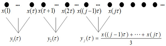
Figure 1.
The coarse-grained process of time series for scale factor .
2. The FE of each coarse-grained time series can be computed according to Equations (1)–(9) and MFE is expressed by Equation (11) as a function of scale factor . This procedure is called MFE analysis.
Here, parameter , is the standard deviation of the original time series, and it is calculated by . Here, .
2.3. Support Vector Machine
The theory of Support Vector Machines (SVM) has received much attention in recent years. The basic idea of SVM is as follows. In the first place, it maps input points to a high dimensional feature space by nonlinear transformation and then finds an optimal classification hyperplane by maximizing the margin between two classes in this space. In this paper, SVM is chosen as a classifier to recognize MI-EEG and the radial basis function is selected as the kernel function. Furthermore, the parameters of SVM, including the kernel parameter and the error penalty factor, are optimized by using traversal searching method.
3. Description of Feature Extraction
Based on the idea of independent optimization of parameters, the normal MFE is improved, and the improved MFE (IMFE) method is applied to the feature extraction of MI-EEG. The specific steps can be summarized as follows:
1. The optimal selection of time interval for MI-EEG
Suppose that the original MI-EEG signal of the Lth channel in a trial is , where and are the number of channels and sampling points per trial, respectively. The FE time series of every channel of MI-EEG is calculated for each training sample of different imaginary tasks. To obtain the mean FE time series, they are superimposed and then averaged for every imaginary task. The optimal sampling interval may be determined to ensure there is a significant difference between the mean fuzzy entropies of MI-EEG on two channels for every imaginary task. A new EEG signal can be constituted by selecting the optimal sampling interval of the data points from the original EEG signal and it can be expressed as , where is the first selected point from , is the last selected point from , is the number of selected data points from , and .
2. The Coarse-Grained Procedure of MI-EEG
The coarse-grained MI-EEG signals of on multiple scale factors can be obtained according to Section 2.2 and denoted as in turn, where , is the maximum of scale factor and represents the coarse-grained MI-EEG of the Lth channel for the jth scale.
3. The Calculation of MFE
The FE of each coarse-grained MI-EEG signal can be calculated according to Section 2.1. The FE of coarse-grained sequences can be denoted as , in turn. Thus, the MFE of the Lth channel MI-EEG is given by Equation (12):
4. The parameters’ independent optimization of MFE for different scale factors
On different scale factors, the parameters, including embedding dimension , boundary gradient , and boundary width , will directly influence the MFE value. To obtain the feature vectors that are beneficial to classification, the relevant parameters will be optimized independently. For multiple scale factors , when any two parameters of , , and remain relatively fixed, the variation curves of the average and standard deviation of MI-EEG’s MFE with a parameter are calculated for different imaginary tasks, respectively. The optimal values of the parameters may be determined by considering the fluctuation of the error line for each imaginary task, the overlapping degree of error lines, and the difference of means between different tasks. After the independent optimization of the parameters, the MFE of the Lth channel MI-EEG is expressed as
where represents the improved FE of the Lth channel MI-EEG for scale factor .
5. The construction of feature vector
The improved multiscale fuzzy entropies of MI-EEG signals on all channels are fused serially to construct a feature vector, or based on the characteristics of MI-EEG, their improved multiscale fuzzy entropies on relevant channels are organically fused. Only the feature vector after serial fusion is given by Equation (14):
where represents the feature vector of MI-EEG in a trial.
4. Experimental Research
4.1. Data Source
The experimental data were derived from dataset III of Brain Computer Interface (BCI) Competition II provided by BCI Lab, Graz University of Technology in Graz, Austria (http://www.bbci.de/competition/ii/). The dataset was obtained by collecting the EEG signals of a healthy adult female while she was imagining left hand or right hand movement. The dataset was composed of 280 trials, of which 140 were used for training and 140 were used for testing. The 140 trials used for training and testing included 70 trials imagining left hand movement and 70 trials imagining right hand movement. Each trial lasted for 9 s, and the timing diagram of the experiment is shown schematically in Figure 2.
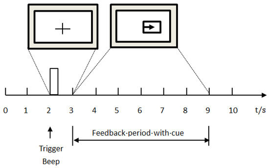
Figure 2.
The timing diagram of the collection experiment.
As shown in Figure 2, for the first two seconds the subject remained quiet and relaxed; when the time reached 2 s, a short beep indicated the start of the trial and the ‘+’ cursor appeared on the monitor simultaneously. When the time was 3–9 s, the visual cue (left–right arrow) was displayed as the direction of motor imagery. At the same time, the subject imagined the hand movement according to the direction indicated by the arrow. The data were sampled at 128 Hz. The three channels, C3, Cz, and C4, were applied to acquire EEG, using Ag/AgCl as an electrode, and the placement of the electrode is shown in Figure 3.
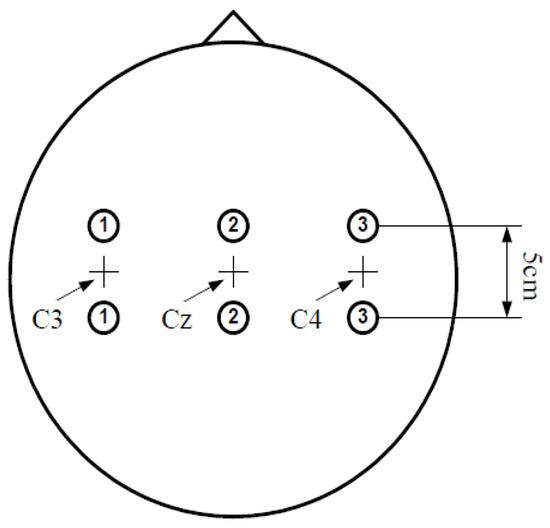
Figure 3.
Electrode placement.
4.2. Optimal Selection of Time Interval for MI-EEG
The MI-EEG signals on channels C3 and C4 from 280 trials of samples were selected as the experimental data. Based on the event-related desynchronization (ERD)/event-related synchronization (ERS) phenomenon associated with hand movement or imaging movement, the optimal sampling interval of MI-EEG may be determined to ensure there is a significant difference between fuzzy entropies corresponding to two motor imaginary tasks. First, for 140 trials of imaginary left hand movement EEG signals on channel C3, the FE time series of each MI-EEG could be obtained by using a sliding time window, where the window length was 1 s, the interval was one sampling point, and parameters , , and were set to 2, 2, and 0.1 SD, respectively. Next, the 140 FE time series of imaginary left hand movement EEGs on channel C3 were superimposed, and averaged to obtain their mean FE time series. In a similar way, the mean FE time series of 140 trials of imaginary left hand movement MI-EEGs on channel C4 could be calculated. Furthermore, the mean FE time series of 140 trials of imaginary right hand movement MI-EEGs on channels C3 and C4 were obtained as well. The experimental results are shown in Figure 4. The solid magenta line represents the mean FE time series of 140 trials of MI-EEG on channel C3 for each imaginary task, and the green dotted line expresses the mean FE time series of 140 trials of MI-EEG on channel C4 for each imaginary task.
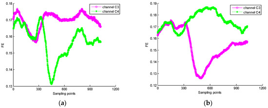
Figure 4.
(a) The mean FE time series of MI-EEG on channels C3 and C4 for imaginary left hand movement; (b) the mean FE time series of MI-EEG on channels C3 and C4 for imaginary right hand movement.
As seen in Figure 4, the means of FE on channels C3 and C4 also change with the variation of sampling point for any one of two imaginary tasks. When the sampling interval is [451,900], the difference of mean FE values between C3 and C4 channels is remarkable. In this paper, the sampling interval will be chosen in the following feature extraction of MI-EEG.
4.3. Multiscale Analysis
The entropy of time series is usually used to characterize its complexity, but the entropy variation of some sequences may be inconsistent on different scale factors. If the majority of scales’ entropy values are higher for one time series than for another, the former is considered more complex than the latter.
We randomly selected two trials of MI-EEG signals on channel C3, in which one is derived from imaginary left hand movement and the other is derived from imaginary right hand movement. Then, we calculated MFE values of two trials of MI-EEG signals. At this time, was equal to 4 and in the calculation of MFE values on different scale factors, the parameters , , and were set to 2, 2, and 0.1 SD, respectively. Here, SD was the standard deviation of the original MI-EEG signal. The experimental result is shown in Figure 5.
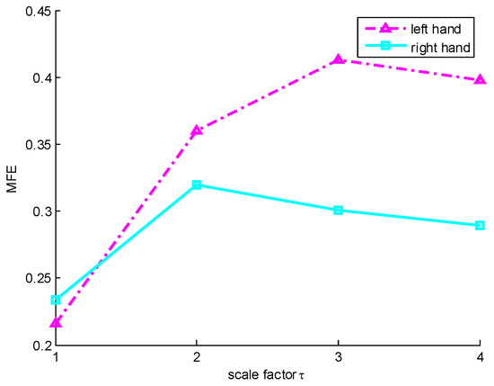
Figure 5.
The MFE variation curves with scale factor . The pink dotted line and blue solid line represent the MFE of MI-EEG on channel C3 corresponding to imaginary left hand and right hand movement, respectively.
From Figure 5, we can see that the FE of MI-EEG signal for imaginary left hand movement is smaller than the FE of MI-EEG signal for imaginary right hand movement when . This means that the latter is more complex than the former. However, when , 3 and 4, the FE values of the MI-EEG signal for imaginary left hand movement are all higher than those of the MI-EEG signal for imaginary right hand movement corresponding to one scale factor; this shows that the former is more complex than the latter. So, it is unreasonable to analyze the complexity of a time series on a single scale with FE. In addition, it can be seen that the coarse-grained MI-EEG signal on each scale factor contains important information related to the imaginary task. To obtain more information, it is necessary for MI-EEG to conduct multiscale analysis.
4.4. Construction of Feature Vector
After performing multiscale analysis for MI-EEG on all channels, a variety of forms can be used to construct the feature vector. If the multiscale fuzzy entropies of MI-EEG on all channels are fused serially, the feature vector is obtained by Equation (15):
where is the maximum of ; , and can be calculated by Equation (12) and stand for the MFE of MI-EEG on channels C3, C4, and Cz, respectively.
Considering the ERD/ERS phenomenon of MI-EEG on channels C3 and C4, we can also flexibly select the MFE values of MI-EEG on those channels to construct a feature vector after a specific operation to guarantee the sharp distinction between two imaginary tasks. The result is as shown in Equation (16):
In calculations for fuzzy entropy on different scale factors, parameters , , and were set to 2, 2, and 0.1 SD, respectively; SD was the standard deviation of the original MI-EEG signal, and was equal to 4.
To find the best means of feature vector construction, some experiments were conducted on a public dataset using SVM as a classifier. In addition, to eliminate the contingency in the feature extraction process and increase the objectivity of feature evaluation, 10-fold Cross-Validation (CV) was employed. This means that the data, including 280 trials, were randomly divided into 10 subsets, each of which was used as a validation set. Experiment environment: Win7 operating system, memory 4G, programming language is Matlab R2014a. The experiment results of 10-fold CV are listed in Table 1.

Table 1.
Comparison of feature vector construction.
Table 1 shows that the feature vector constructed by Equation (16) has certain advantages over constructed by Equation (15), and the highest classification accuracy and average classification rate with 10-fold CV were 100% and 90.36%, respectively. It is obvious that the feature vector is more conducive to mining and characterizes more and deeper feature information contained in the MI-EEG signal. Therefore, feature vector is employed in the following experiments.
4.5. The Parameters’ Independent Optimization of MFE
In the course of calculating MFE, the four parameters, i.e., scale factor , embedding dimension , boundary gradient , and boundary width , should be determined in advance. For scale factor , when it was too large, the calculation of MFE would raise the problem of insufficient data points, while a too small scale factor would not be good for accessing the deeper information of MI-EEG. From Section 4.2 we can see that the change of FE is significant when the time range is [451,900]. Meanwhile, to ensure that the calculation of FE is not affected by the data length, the length of time series is at least 100 points. As a result, was set to 4. The remaining three parameters would be determined by experiments. Firstly, when , , , and were given fixed values, we calculated the fuzzy entropy of 140 trials of MI-EEG on channel C3 and C4 for imaginary left hand movement. Then, we calculated 140 differences between the FE on channel C3 and the FE on channel C4, and we defined , where and stand for the FE of MI-EEG on channels C3 and C4, respectively. Finally, we calculated the mean and standard deviation of 140 , and they were noted as and , respectively. For a given , we could obtain the variation curve of and with any one parameter while the others were kept constant. When scale factor was 1, we obtained three curves, which are presented in Figure 6. The solid pink line represents the situation of imaginary left hand movement. Similarly, the results associated with imaginary right hand movement are displayed with a green dotted line.
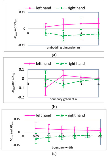
Figure 6.
For , the mean and standard deviation of FED curves for input variables (a) embedding dimension ; (b) boundary gradient ; and (c) boundary width .
Figure 6a gives the variation curves of and with parameter when , and is the standard deviation of original MI-EEG. When equals 1, although is small for any one of the imaginary tasks, which means the MI-EEG signals are more intensive for any one of two tasks, the values corresponding to two imaginary tasks are quite close, which means the two tasks show a poor distinction. With the increase of , for any one of two imaginary tasks the first increases and then remains stable. The bigger is, the more accurate the calculation of FE is and the more detailed information is implied. Meanwhile, the more complex the computation, the more data points are needed. Taking into account the constraints of the experimental dataset, the parameter is set to 2. Figure 6b displays the variations of and with parameter when , and SD is the standard deviation of the original MI-EEG. When parameter is 1, the values corresponding to the two imaginary tasks are quite different, which means they show a better distinction, but the values are also very big for the two tasks, which means the MI-EEG signal is too scattered for any one task. When parameter equals 3 or 4, is small for any one imaginary task. On the other hand, the values corresponding to the two imaginary tasks are very close. When parameter equals 2, is moderate for any one imaginary task; meanwhile the values corresponding to the two imaginary tasks are quite different. To sum up, the parameter is set to 2. Figure 6c exhibits variations of and with parameter when . The values corresponding to the two imaginary tasks are quite different, while the values for the two tasks are both large when parameter is relatively small. With the increase of , the corresponding to the two imaginary tasks become smaller. In conclusion, the parameter is selected as , and SD is the standard deviation of the original MI-EEG.
In summary, when scale factor is 1, the values of parameters , and have a significant influence on the FE of MI-EEG for two imaginary tasks, and this will directly affect the quality of the FE features. Therefore, it is necessary to further optimize the parameters of FE when scale factor equals 2, 3, and 4. The and values with different parameters , and are obtained by using a similar computation process, and their variations are shown in Figure 7, Figure 8 and Figure 9, respectively.
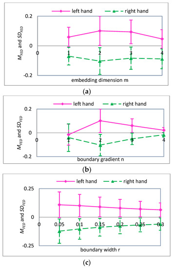
Figure 7.
For , the mean and standard deviation of FED curves for input variables (a) embedding dimension ; (b) boundary gradient ; and (c) boundary width .
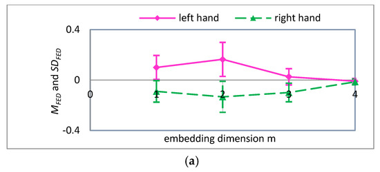
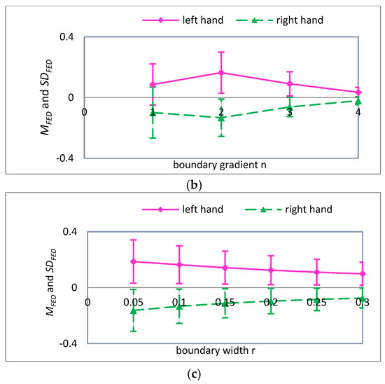
Figure 8.
For , the mean and standard deviation of FED curves for input variables (a) embedding dimension ; (b) boundary gradient ; and (c) boundary width .
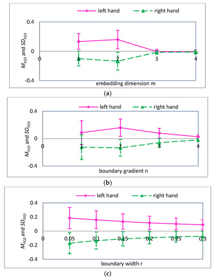
Figure 9.
For , the mean and standard deviation of FED curves for input variables (a) embedding dimension ; (b) boundary gradient ; and (c) boundary width .
A detailed analysis of Figure 7, Figure 8 and Figure 9 was performed using the analysis method of Figure 6. It can be seen that the parameters are more suitable for the classification of MI-EEG when , and 4. Note that SD is the standard deviation of the coarse-grained MI-EEG corresponding to each scale factor , and not the standard deviation of the original MI-EEG.
To prove the necessity of parameter optimization, a comparison between IMFE and MFE was carried out on a public dataset and SVM was chosen as a classifier. In the computation of MFE, were selected, but SD was different in the two methods. In the IMFE method, SD was the standard deviation of the coarse-grained MI-EEG corresponding to each scale factor , i.e., SD was varied with . However, in the MFE method, SD was the standard deviation of the original MI-EEG on each scale factor and was constant. The experimental results are listed in Table 2.
Table 2.
The influence of parameter optimization in MFE on recognition rate.
As seen from Table 2, when IMFE is employed to extract the feature of MI-EEG, the average classification rate with 10-fold CV increases by 1.78% from 90.36% to 92.14% compared with MFE, and the experimental results of IMFE show more stability than MFE. This demonstrates that the parameters’ independent optimization of MFE is beneficial for enhancing the accuracy and adaptability of the feature extraction method.
4.6. Comparison of Multi-Feature Extraction Methods
To compare IMFE with the nonlinear dynamic methods and the classical feature extraction methods, some experiments were conducted on a public dataset using SVM as a classifier.
4.6.1. Comparison with Multiple Nonlinear Dynamic Methods
The proposed IMFE and the other nonlinear dynamic methods, including ApEn, SampEn, FE, PE, WPE, MSE, MPE, and MFE, were used to extract the features of MI-EEG. The experimental results are given in Figure 10.
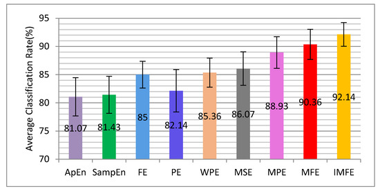
Figure 10.
The average classification accuracy and standard deviation performed by 10-fold CV for IMFE and multiple nonlinear dynamic methods.
As seen from Figure 10, the classification results of ApEn and SampEn are relatively poor, because they use the Heaviside function to measure the similarity definition of reconstructed vectors. FE replaces the Heaviside function with fuzzy membership function, and the recognition rate has been improved. The classification accuracy of WPE is higher than that of PE. This is because WPE also contains amplitude information besides the order structure of MI-EEG, compared with PE. Compared with ApEn, SampEn, FE, and PE, the classification rates of MSE, MPE, and MFE have been greatly improved. That is because ApEn, SampEn, FE, and PE can only estimate the complexity of time series based on a single scale and MSE, MPE, and MFE can measure the complexity of time series on multiple scale factors. IMFE is improved by adding the parameters’ independent optimization to MFE, and it can adaptively extract more and deeper information so that the classification accuracy can be further improved. In addition, compared to other nonlinear dynamic methods, its standard deviation (±2.1) is the smallest, which means that the improved MFE method has better stability.
4.6.2. Comparison with Multiple Classical Feature Extraction Methods
In this section, some experiments were carried out to compare the proposed IMFE with classical feature extraction methods, including AR, WT, CSP, CSSP, and FBCSP. In the experiments, the parameter values of AR and WT were the same as the reference [3,4], respectively. The parameter values of CSP, CSSP, and FBCSP were the same as the reference [34]. The average classification accuracies with 10-fold CV are shown in Figure 11.
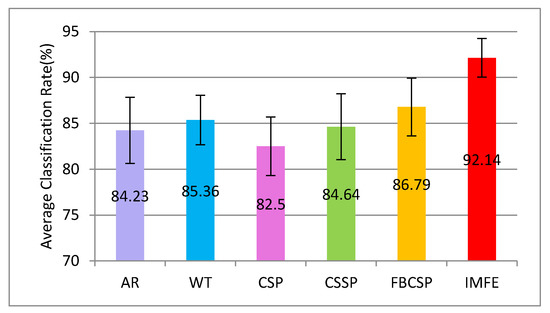
Figure 11.
The average classification accuracy and standard deviation performed by 10-fold CV for IMFE and multiple classical feature extraction methods.
The classification results of AR, WT, CSP, CSSP, and FBCSP are not as good as those of the IMFE method. This is mainly because these classical feature extraction methods only take into account the information in one domain, including time domain, frequency domain or spatial domain, and they are even completed on the premise that MI-EEG is a linear signal. In fact, MI-EEG is a typical nonlinear signal. IMFE is matched with the nonlinear property of signal, and the parameters’ independent optimization of MFE is advantageous for accurately extracting and correctly interpreting the characteristic information of MI-EEG. Furthermore, the minimal standard deviation of IMFE (±2.1) shows the strong stability, and this can better meet the requirements of a real application.
4.7. Comparison of Multiple Recognition Methods
In this section, a comparative study was performed on the same public dataset to prove the effectiveness of the recognition method, i.e., the combination of IMFE and SVM.
First, the combined recognition of IMFE and SVM was compared with the top three methods in BCI competition II in many aspects [35]. The detailed information is illustrated in Table 3.
Table 3.
Comparison with the top three recognition methods in BCI competition II.
From Table 3, it can be seen that the highest recognition rate of 100% is achieved by using IMFE feature extraction and the SVM classifier; it has increased significantly compared with the top three methods. Furthermore, the average recognition rate with 10-fold CV is higher than the highest recognition rates of the other three methods.
Next, some research was completed about the combined recognition of IMFE and SVM and the other recognition methods, whose experimental data was from the same dataset III of BCI Competition II [4,36,37,38,39,40,41,42,43,44,45,46,47,48,49]. The detailed information, including the reference numbers, feature extraction methods, classifiers, etc., is shown in Table 4.
Table 4.
Comparison with other recognition methods.
From Table 4, we can see that the proposed recognition method has the highest classification rate (100%) and its average recognition rate (92.14%) with 10-fold CV is higher than the highest recognition rates corresponding to the other methods except references [4,40,49].
4.8. Computation Time
The computation time can actually reflect the complexity of a method, and it is closely related to the application in a BCI system. Figure 12 presents the test time of feature extraction in a trial by using the proposed IMFE method and the conventional feature extraction methods (AR, WT, CSP, CSSP, FBCSP, ApEn, SampEn, FE, PE, WPE, MSE, and MPE). Less time is consumed in application of AR, WT, CSP, CSSP, and ApEn, but their effect of feature extraction is not ideal, as we know from the above analysis. The time consumption of SampEn, PE, WPE, MSE, and MPE is at a medium level. FBCSP, FE, and IMFE need more time, especially IMFE, which means that IMFE has a relatively higher computational complexity compared to the other methods. This is mainly because of the exponential membership function in IMFE. However, it could basically satisfy the requirements of a BCI system.
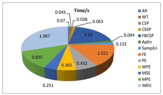
Figure 12.
A comparison of time consumption using the proposed IMFE and conventional feature extraction methods.
4.9. Statistical Analysis
The IMFE is developed in this paper on the basis of MFE. It is necessary to analyze the differences between IMFE and MFE statistically. In the following, a paired t-test is applied to identify whether there is a significant difference when they are used for feature extraction of MI-EEG.
Suppose that and stand for the improved fuzzy entropy of the Lth channel MI-EEG for scale factor corresponding with imaginary left hand and right hand movements, respectively. Similarly, and denote the normal fuzzy entropy of the Lth channel MI-EEG for scale factor corresponding with imaginary left hand and right hand movements, respectively. Define , , and , and calculate D for each channel of C3, C4, and Cz and each one of scale factor . Then, we tested that D is a sample from a normal population . The null hypothesis is ; the alternative hypothesis is . The one-tailed paired t-test was chosen (). The decision rule is to reject if:
or
where and denote the mean and standard deviation of sample , respectively; is the number of elements in sample . The t-test results are shown in Table 5.
Table 5.
Paired t-test results.
From Table 5, we see that all the p values are less than 0.05. Therefore, the null hypothesis is rejected at the 0.05 significance level. Therefore, the fuzzy entropy values obtained by IMFE and MFE are significantly different and IMFE outperforms MFE in discriminating between two imaginary tasks.
5. Conclusions
Aiming at the highly nonlinearity and multiscale property of MI-EEG, MFE is introduced and improved to measure its complexity. Especially with the parameters’ independent optimization strategy, all the parameters of MFE are optimized for each scale factor in sequence. So, the MFE of each coarse-grained MI-EEG on a different scale factor is calculated by using different parameter values. This makes IMFE a more accurate multiscale analysis method. It would be helpful to discover the nature of a nonlinear signal in more detail. The improved MFE is applied to the feature extraction of MI-EEG, and results in relatively higher classification accuracy compared with the exiting nonlinear dynamic methods and conventional time, frequency, or spatial domain analysis methods. The statistical results of a paired t-test further illustrate that IMFE has significant advantages over MFE. These lay the foundation for expanding the application of nonlinear dynamic methods in EEG or even other bioelectrical signals. However, IMFE requires relatively more computation time than some other methods. This is mainly due to the exponential fuzzy membership function in MFE. We will solve that problem by simplifying the fuzzy membership function and improving programming skills in future work.
Acknowledgments
This work was financially supported by the National Natural Science Foundation of China (No. 81471770), the Natural Science Foundation of Beijing (No. 7132021), and the Integrated Promotion Project of Beijing University of Technology. We would like to thank all of the people who have given us helpful suggestions and advice. The authors are obliged to the anonymous referees for carefully looking over the details and for useful comments that improved this paper.
Author Contributions
Hai-na Liu conceived the study; Ming-ai Li and Hai-na Liu conducted the experiments and analyzed the results; Hai-na Liu wrote the manuscript; Ming-ai Li, Wei Zhu and Jin-fu Yang helped revise the paper.
Conflicts of Interest
The authors declare no conflict of interest.
References
- Ang, K.K.; Chua, K.S.; Phua, K.S.; Wang, C.; Chin, Z.Y.; Kuah, C.W. A randomized controlled trial of EEG-based motor imagery brain-computer interface robotic rehabilitation for stroke. Clin. EEG Neurosci. 2015, 46, 310–320. [Google Scholar] [CrossRef] [PubMed]
- Zhang, H.; Yang, H.; Guan, C. Bayesian learning for spatial filtering in an EEG-based brain-computer interface. IEEE Trans. Neural Netw. Learn. Syst. 2013, 24, 1049–1060. [Google Scholar] [CrossRef] [PubMed]
- Zhang, Y. Recognition of motor imagery EEG based on AR and SVM. J. Huazhong Univ. Sci. Technol. 2011, 39, 103–106. [Google Scholar]
- Li, M.A.; Wang, R.; Hao, D.M. Feature extraction and classification of EEG for imagery left-right hands movement. Chin. J. Biomed. Eng. 2009, 28, 166–170. [Google Scholar]
- Boonnak, N.; Kamonsantiroj, S.; Pipanmaekaporn, L. Wavelet transform enhancement for drowsiness classification in EEG records using energy coefficient distribution and neural network. Int. J. Mach. Learn. 2015, 5, 288–293. [Google Scholar] [CrossRef]
- Nasihatkon, B.; Boostani, R.; Jahromi, M.Z. An efficient hybrid linear and kernel CSP approach for EEG feature extraction. Neurocomputing 2009, 73, 432–437. [Google Scholar] [CrossRef]
- Dornhege, G.; Blankertz, B.; Krauledat, M.; Losch, F.; Curio, G.; Müller, K.R. Combined optimization of spatial and temporal filters for improving brain-computer interfacing. IEEE Trans. Biomed. Eng. 2006, 53, 2274–2281. [Google Scholar] [CrossRef] [PubMed]
- Lemm, S.; Blankertz, B.; Curio, G.; Müller, K.R. Spatio-spectral filters for improving the classification of single trial EEG. IEEE Trans. Biomed. Eng. 2005, 52, 1541–1548. [Google Scholar] [CrossRef] [PubMed]
- Novi, Q.; Guan, C.; Dat, T.H.; Xue, P. Sub-band common spatial pattern (SBCSP) for brain-computer interface. In Proceedings of the 3rd International IEEE EMBS Conference on Neural Engineering, Kohala Coast, HI, USA, 2–5 May 2007.
- Kai, K.A.; Zheng, Y.C.; Zhang, H.; Guan, C. Filter Bank Common Spatial Pattern (FBCSP) in Brain-Computer Interface. In Proceedings of the IEEE International Joint Conference on Neural Networks, Hong Kong, China, 1–8 June 2008; pp. 2390–2397.
- Pincus, S.M. Approximate entropy as a measure of system complexity. Proc. Natl. Acad. Sci. USA 1991, 88, 2297–2301. [Google Scholar] [CrossRef] [PubMed]
- Vega, C.H.; Noel, J.; Fernandez, J.R. Cognitive task discrimination using approximate entropy (ApEn) on EEG signals. In Proceedings of the 2013 ISSNIP Biosignals and Biorobotics Conference (BRC), Rio de Janeiro, Brazil, 18–20 February 2013; pp. 1–4.
- Zhang, Z.; Du, S.H.; Chen, Z.Y.; Tian, X.H.; Zhou, Y.; Zhang, Y. The application of approximate entropy and support vector machine in classifying signal of epilepsy. J. Biomed. Eng. Res. 2013, 32, 74–79. [Google Scholar]
- Richman, J.S.; Moorman, J.R. Physiological time-series analysis using approximate entropy and sample entropy. Am. J. Physiol. Heart Circ. Physiol. 2000, 278, 2039–2049. [Google Scholar]
- Zhou, P.; Ge, J.Y.; Cao, H.B.; Zhang, S.; Wang, M.S. Classification of motor imagery based on sample entropy. Inf. Control 2008, 37, 191–196. [Google Scholar]
- Wang, L.; Xu, G.Z.; Yang, S.; Wang, J.; Guo, M.M.; Yan, W.L. Motor Imagery BCI Research Based on Sample Entropy and SVM. In Proceedings of the 2012 Sixth International Conference on Electromagnetic Field Problems and Applications (ICEF), Dalian, China, 19–21 June 2012; pp. 1–4.
- Chen, W.T.; Zhuang, J.; Yu, W.X.; Wang, Z.Z. Measuring complexity using FuzzyEn, ApEn, and SampEn. Med. Eng. Phys. 2009, 31, 61–68. [Google Scholar] [CrossRef] [PubMed]
- Tian, J.; Luo, Z.Z. Motor imagery EEG feature extraction based on fuzzy entropy. J. Huazhong Univ. Sci. Technol. 2013, 41, 92–95. [Google Scholar]
- Xu, L.Q.; Liu, J.X.; Xiao, G.C.; Jin, W.D. Characterization and classification of EEG attention based on fuzzy entropy. J. Comput. Appl. 2012, 32, 3268–3270. [Google Scholar]
- Bandt, C.; Pompe, B. Permutation entropy: A natural complexity measure for time series. Phys. Rev. Lett. 2002, 88, 1–5. [Google Scholar] [CrossRef] [PubMed]
- Bruzzo, A.A.; Gesierich, B.; Santi, M.; Tassinari, C.A.; Birbaumer, N.; Rubboli, G. Permutation entropy to detect vigilance changes and preictal states from scalp EEG in epileptic patients. A preliminary study. Neurol. Sci. 2008, 29, 3–9. [Google Scholar] [CrossRef] [PubMed]
- Nicolaou, N.; Georgiou, J. The use of permutation entropy to characterize sleep electroencephalograms. Clin. EEG Neurosci. 2011, 42, 24–28. [Google Scholar] [CrossRef] [PubMed]
- Fadlallah, B.; Chen, B.; Keil, A.; Príncipe, J. Weighted-permutation entropy: A complexity measure for time series incorporating amplitude information. Phys. Rev. E. 2013, 87, 1647–1650. [Google Scholar] [CrossRef] [PubMed]
- Mammone, N.; Duunhenriksen, J.; Kjaer, T.; Morabito, F. Differentiating interictal and ictal states in childhood absence epilepsy through permutation Rényi entropy. Entropy 2015, 17, 4627–4643. [Google Scholar] [CrossRef]
- Costa, M.; Goldberger, A.L.; Peng, C.K. Multiscale entropy analysis of biological signals. Phys. Rev. E. 2005, 71, 1–18. [Google Scholar] [CrossRef] [PubMed]
- Costa, M.; Goldberger, A.L.; Peng, C.K. Multiscale entropy analysis of complex physiologic time series. Phys. Rev. Lett. 2002, 89, 705–708. [Google Scholar] [CrossRef] [PubMed]
- Ge, J.Y.; Zhou, P.; Zhao, X.; Liu, H.Y.; Wang, M.S. Multiscale entropy analysis of EEG signal. Comput. Eng. Appl. 2009, 45, 13–15. [Google Scholar]
- Liu, M.M.; Ai, L.M. Application of multi-scale entropy for detecting driving fatigue in EEG. Comput. Technol. Dev. 2011, 21, 209–212. [Google Scholar]
- Aziz, W.; Arif, M. Multiscale Permutation Entropy of Physiological Time Series. In Proceedings of the 9th International Multitopic Conference, Karachi, Pakistan, 23–24 December 2005.
- Ouyang, G.X.; Li, J.; Liu, X.Z.; Li, X.L. Dynamic characteristics of absence EEG recordings with multiscale permutation entropy analysis. Epilepsy Res. 2013, 104, 246–252. [Google Scholar] [CrossRef] [PubMed]
- Morabito, F.C.; Labate, D.; Foresta, F.L.; Bramanti, A.; Morabito, G.; Palamara, I. Multivariate multi-scale permutation entropy for complexity analysis of Alzheimer’s disease EEG. Entropy 2012, 7, 1186–1202. [Google Scholar] [CrossRef]
- Zheng, J.D.; Chen, M.J.; Cheng, J.S.; Yang, Y. Multiscale fuzzy entropy and its application in rolling bearing fault diagnosis. J. Vib. Eng. 2014, 27, 145–151. [Google Scholar]
- Azami, H.; Escudero, J. Refined composite multivariate generalized multiscale fuzzy entropy: A tool for complexity analysis of multichannel signals. Physica A 2017, 465, 261–276. [Google Scholar] [CrossRef]
- Li, M.A.; Guo, S.D.; Yang, J.F. A novel EEG feature extraction method based on OEMD and CSP algorithm. J. Intell. Fuzzy Syst. 2016, 30, 2971–2983. [Google Scholar]
- Blankertz, B.; Müller, K.R.; Curio, G.; Vaughan, T.M.; Schalk, G.; Wolpaw, J.R.; Schlögl, A.; Neuper, C.; Pfurtscheller, G.; Hinterberger, T.; et al. The BCI Competition 2003: Progress and perspectives in detection and discrimination of EEG single trials. IEEE Trans. Biomed. Eng. 2004, 5, 1044–1051. [Google Scholar] [CrossRef] [PubMed]
- Huang, S.J.; Wu, X.M. Feature extraction of electroencephalogram for imagery movement based on Mu/Beta rhythm. J. Clin. Rehabil. 2010, 14, 8061–8064. [Google Scholar]
- Liu, C.; Zhao, H.B.; Li, C.S.; Wang, H. CSP/SVM-based EEG classification of imagined hand movements. J. Northeast. Univ. 2010, 31, 1098–1101. [Google Scholar]
- Wu, Y.; Ge, Y.B. A novel method for motor imagery EEG adaptive classification based biomimetic pattern recognition. Neurocomputing 2013, 116, 280–290. [Google Scholar] [CrossRef]
- Su, S.J.; Fang, H.J.; Wang, G. EEG features extraction based on multi-parameter common spatio-spectral pattern algorithm. Microcomput. Appl. 2011, 30, 72–75. [Google Scholar]
- Xu, B.G.; Song, A.G.; Fei, S.M. Pattern recognition method of motor imagery tasks. Chin. J. Sci. Instrum. 2011, 32, 13–18. [Google Scholar]
- Wang, Y.R.; Li, X.; Li, H.H.; Shao, C.C.; Ying, L.J.; Wu, S.C. Feature extraction of motor imagery electroencephalography based on time-frequency-space domains. J. Biomed. Eng. 2014, 31, 955–961. [Google Scholar]
- Ren, Y.L. Electroencephalogram recognition of imaginary right and left hand movements by brain-computer interface. J. Clin. Rehabil. 2009, 13, 3370–3374. [Google Scholar]
- Li, F.; Qiu, T.S.; Ma, Z. Study on wavelet feature extraction and semi-supervised recognition of brain signal. Chin. J. Biomed. 2010, 29, 650–653. [Google Scholar]
- Li, D.M.; Wang, D.H.; Yan, J.; Wang, Y.T.; Song, M.L.; Yu, B.B. Movement imagery electroencephalogram recognition based on MOWDT. Comput. Eng. 2014, 10, 161–167. [Google Scholar]
- Zhang, X.P.; Fan, Y.L.; Yang, Y. On the classification of consciousness tasks based on the EEG singular spectrum entropy. Comput. Eng. Sci. 2009, 31, 117–120. [Google Scholar]
- Ren, Y.L. Applying wavelet packet entropy and BP neural networks in recognition of mental tasks. Comput. Appl. Softw. 2009, 26, 78–81. [Google Scholar]
- Yu, W.; Wan, D.L.; Yang, X.J.; Zhou, Y. An improved FCM algorithm and its application to EEG signal processing. J. Chongqing Univ. 2014, 37, 83–89. [Google Scholar]
- Yu, W.; Han, Q.; Ma, J.J.; Xie, P. EEG signal processing method based on EMD and SVM. J. Kunming Univ. Sci. Technol. 2012, 37, 38–42. [Google Scholar]
- Li, M.A.; Tian, X.X.; Sun, Y.J.; Yang, J.F. Adaptive recognition method based on improved-GHSOM for motor imagery EEG. Chin. J. Sci. Instrum. 2015, 36, 1064–1071. [Google Scholar]
© 2017 by the authors; licensee MDPI, Basel, Switzerland. This article is an open access article distributed under the terms and conditions of the Creative Commons Attribution (CC-BY) license (http://creativecommons.org/licenses/by/4.0/).