Article

Piecewise Function Hysteretic Model for Cold-Formed Steel Shear Walls with Reinforced End Studs

School of Civil Engineering, Southeast University, Nanjing 210096, China
*
Author to whom correspondence should be addressed.
Appl. Sci. 2017, 7(1), 94; https://doi.org/10.3390/app7010094
Submission received: 9 November 2016 / Revised: 10 January 2017 / Accepted: 11 January 2017 / Published: 19 January 2017
(This article belongs to the Special Issue Applications of Thin-Walled Structures)

Abstract

:
Cold-formed steel (CFS) shear walls with concrete-filled rectangular steel tube (CFRST) columns as end studs can upgrade the performance of mid-rise CFS structures, such as the vertical bearing capacity, anti-overturning ability, shear strength, and fire resistance properties, thereby enhancing the safety of structures. A theoretical hysteretic model is established according to a previous experimental study. This model is described in a simple mathematical form and takes nonlinearity, pinching, strength, and stiffness deterioration into consideration. It was established in two steps: (1) a discrete coordinate method was proposed to determine the load-displacement skeleton curve of the wall, by which governing deformations and their corresponding loads of the hysteretic loops under different loading cases can be obtained; afterwards; (2) a piecewise function was adopted to capture the hysteretic loop relative to each governing deformation, the hysteretic model of the wall was further established, and additional criteria for the dominant parameters of the model were stated. Finally, the hysteretic model was validated by experimental results from other studies. The results show that elastic lateral stiffness Ke and shear capacity Fp are key factors determining the load-displacement skeleton curve of the wall; hysteretic characteristics of the wall with reinforced end studs can be fully reflected by piecewise function hysteretic model, moreover, the model has intuitional expressions with clear physical interpretations for each parameter, paving the way for predicting the nonlinear dynamic responses of mid-rise CFS structures.

1. Introduction

As the main load-bearing components of cold-formed steel (CFS) structures, the definition of a CFS shear wall’s hysteretic model is essential for nonlinear dynamic analysis of the structures. At present, full-scale cyclic loading tests are the main way to investigate the shear performance of CFS shear wall, and the definition of the walls’ hysteretic characteristics depends largely on test results [1,2,3,4,5,6,7,8], because those walls have complex configurations and their load-displacement curves exhibit high nonlinearity and pinching together with strength and stiffness deterioration. However, cyclic loading tests fall short with high costs and long experimental periods, amongst other shortcomings; furthermore, the test curves are too complicated to be directly applied in nonlinear analyses of the structures. Therefore, it is necessary to establish a hysteretic model, which can not only be described with simple mathematical expressions, but also reflect the hysteretic characteristics of the wall in order to predict the nonlinear dynamic responses of CFS structures. So far, numerous numerical studies have been conducted on the seismic performance of traditional CFS shear walls with coupled C section end studs [9,10,11,12,13,14].
Currently available hysteretic models for the shear behavior of CFS shear wall include Bouc-Wen-Baber-Noori (BWBN) model, evolutionary parameter hysteretic model (EPHM), pivot model, and three-segment nonlinear pinching hysteretic model [5,6,7,8,9]. The BWBN model was proposed by Foliente [15] and Nithyadharan and Kalyanaraman [16] based on a single-degree-of-freedom (SDOF) mechanical system of a CFS shear wall; the model can fully reflect the wall’s hysteretic characteristics although its mathematical expression which adopts the use of a differential equation cannot obtain an analytical solution, and parameter identification requires a specific algorithm. EPHM, which was proposed by Pang et al. [17] can reveal the effect of loading history on a wall’s lateral stiffness although it lacks a good reflection of pinching, also, loading stiffness increases monotonically with the displacement of the wall growing, which differs from reality. Huang et al. [18] and Zhou et al. [19] presented the degraded four-line pivot model and three-segment nonlinear pinching hysteretic model, respectively, both of which can describe the hysteretic characteristics of the wall more completely, although their parameter identification processes depend on experimental results.
Traditional CFS shear walls with coupled C section end studs are apparently not applicable to mid-rise CFS structures, for both shear strength and fire resistance of the wall cannot satisfy the requirements of mid-rise residential structures [20]. Hence, Wang and Ye [21] proposed a CFS shear wall with continuous concrete-filled rectangular steel tube (CFRST) columns as end studs (see Figure 1), in which double-layer wallboards were arranged on both sides with a staggered configuration in order to enhance the vertical bearing capacity, anti-overturning ability, shear strength, and fire resistance of the wall, thereby allowing it to be applied to mid-rise CFS structures. The subjects of the above hysteretic models focus on the traditional CFS shear walls and are thus confined to low-rise CFS structures, narrowing their applications. Consequently, it is necessary to establish a hysteretic model with a good reflection of hysteretic characteristics of walls according to the configuration of CFS shear walls with reinforced end studs in order to facilitate the nonlinear dynamic analysis of mid-rise CFS structures.
A piecewise function hysteretic model of CFS shear walls with reinforced end studs was proposed according to previous experimental hysteretic laws. The very model can fully reflect the relevant hysteretic characteristics (i.e., stiffness deterioration, strength deterioration, and pinching). Approaches to the load-displacement skeleton curve, hysteretic model, and decisive parameters of the wall are presented in detail. Finally, the proposed hysteretic model is validated by the experimental results of Xu [22].

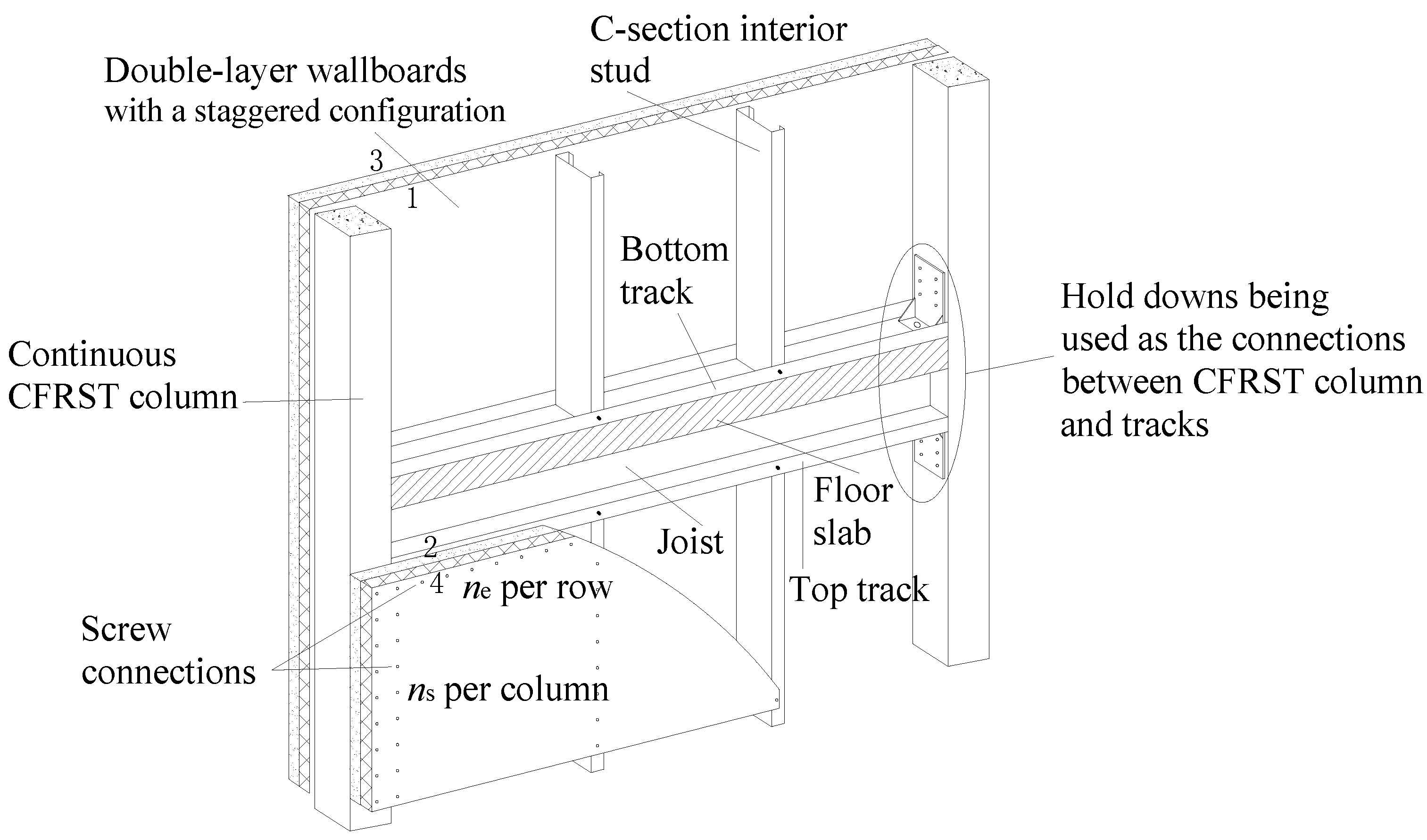
2. Construction and Shear Behavior of CFS Shear Wall with Reinforced End Studs

As shown in Figure 1, a typical CFS shear wall with reinforced end studs consists of a steel frame, sheathings, and screw connections. The steel frame is framed with continuous CFRST columns, C-section interior studs, and U-section tracks; the CFRST column is welded face-to-face along the vertical direction to create a rectangular tube using double CFS lipped channel section studs that are conveniently filled with fine aggregate concrete as soon as the wallboards have been fixed on the frame; a sheathing combination of gypsum wallboards (GWB) and bolivian magnesium boards (BMB), which exhibits good fire performance, is adopted with a staggered configuration; sheathings are attached to the frame using self-drilling screws with a 4.8 mm diameter, and all fastener spacings are 150 mm. In addition, hold downs are placed at the bottom and top of the wall to further strengthen the connection between the CFRST columns and tracks.
An experimental investigation of full-scale CFS shear walls with reinforced end studs, as shown in Figure 1, subjected to cyclic loading was conducted by Wang and Ye [21]. The experimental results indicate that, for screw connections in the perimeter of the walls, the failure modes were either screws being sheared off or screws being pulled through wallboards, both of which were the main reasons for causing the walls’ failure in shear; whereas, no obvious deformation was observed in the screw connections of interior studs. In addition, when the wall became damaged, there were a large number of cross inclined cracks in the base-layer wallboards. It is worth mentioning that the experimental results of CFS shear walls sheathed with ribbed steel plates in shear that were demonstrated by Li et al. [23] also show that the ribbed steel plates had obvious oblique shear buckling. It can be concluded that "tension fields" that were similar to those of the steel plate shear wall were formed in the wallboard when the wall with reinforced end studs was in shear.
Figure 2 describes a typical load-displacement hysteretic curve of the wall with reinforced end studs subjected to cyclic loading. It is observed that the curve of the wall with reinforced end studs has similar pinching characteristic with that of a traditional CFS shear wall with coupled C-section end studs. Screw connections play a governing role in the shear behavior of the wall; once maximum historical displacement of screw connections are exceeded, the screws will squeeze and frictionate the wallboard in the vicinity of the screw holes, resulting in stiffness deterioration of the wall; looseness of those screw holes during cyclic loading generates the slipping and pinching characteristics of the hysteresis curve.

3. Hysteretic Model of CFS Shear Walls with Reinforced End Studs

Based on the hysteretic characteristics of the load-displacement curves discussed in the study by Wang and Ye [21], a hysteretic model of the wall with reinforced end studs will be established in two steps: (1) the load-displacement skeleton curve, which can describe both strength deterioration and stiffness deterioration of the wall, will first be determined as the backbone curve of the hysteretic model; (2) hysteretic loops which can reflect both slipping and pinching characteristics of the wall will be captured in succession, and the hysteretic model will be further established.

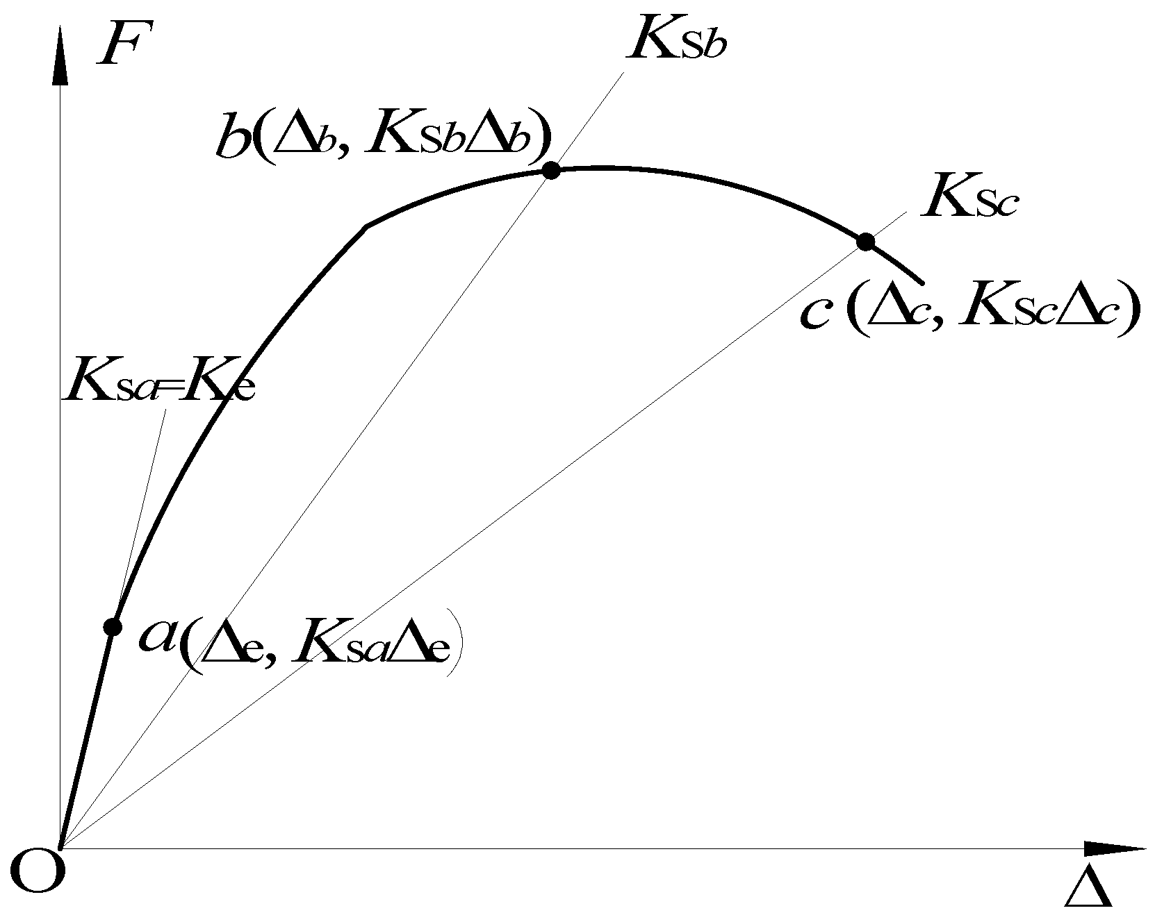
3.1. Modeling of Backbone Curve

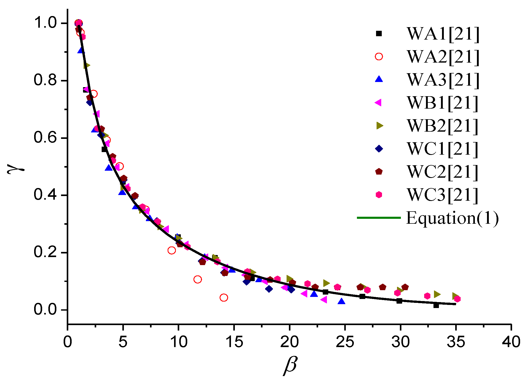
3.1.1. Degradation Analysis of the Lateral Stiffness of the Wall

During horizontal loading, the lateral stiffness of the wall degraded gradually because of the degree of damage to the screw connections that were aggravated with the growing load. In this study, lateral stiffness deterioration was reflected by tracing the secant stiffness of the wall; that is, the average ratio of the loads in two opposite directions of the skeleton curve to their corresponding displacements, respectively, under each load level. Figure 3 depicts the degradation trends of secant stiffness Ks relative to elastic lateral stiffness Ke, in which coincident degradation trends of each specimen can be observed. Therefore, degradation coefficient γ was introduced, which is the ratio of Ks to Ke, to describe the developing trend of the lateral stiffness of the wall. The coefficient, through fitting the test results, is denoted as
γ = K s / K e = 0.623 e 0.098 β + 0.732 e 0.535 β
β = Δ Δ e = Δ K e 0.4 F p
where Ke is the ratio of conventional elastic strength limit Fe = 0.4Fp to its corresponding displacement Δe; β, which can be calculated by Equation (2), which is the ratio of lateral displacement Δ of the wall to Δe; Fp which is the shear capacity of the wall.

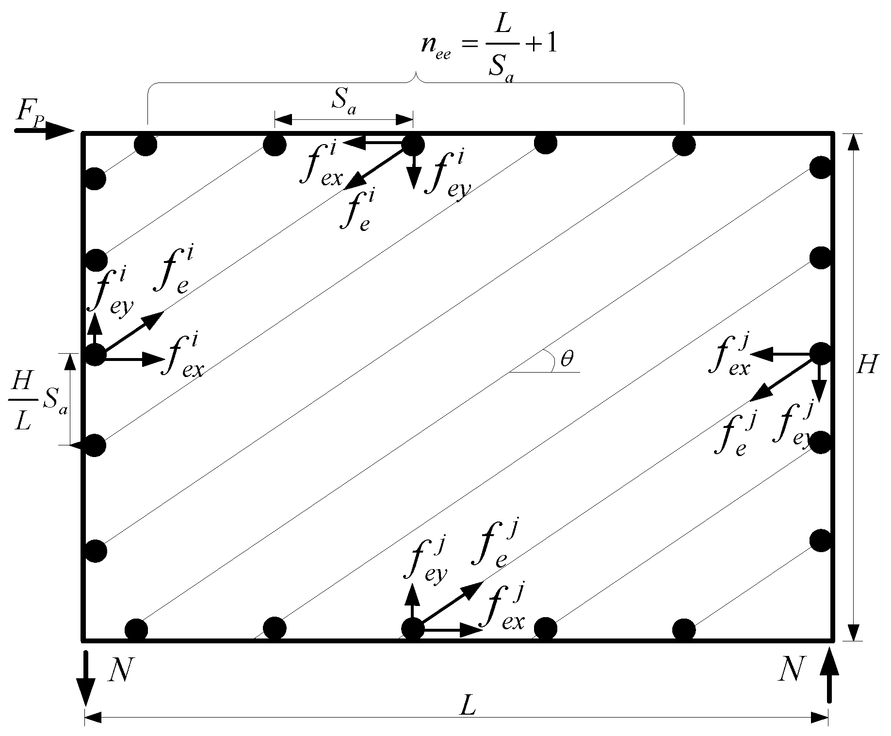
3.1.2. Discrete Coordinate Method

As shown in Figure 4, the load-displacement skeleton curve was discretized into a series of coordinates (a, b, c …). Coordinate a is defined as the elastic point, where it is assumed that the skeleton curve is linear until it has reached the elastic displacement Δe corresponding to coordinate a, with the load relative to the remaining coordinates being a function of the lateral displacement and secant stiffness of the wall. It can be observed from Equations (1) and (2) that given lateral displacement Δ, the secant stiffness corresponding to Δ can be obtained according to the elastic lateral stiffness Ke and shear capacity Fp of the wall, the discrete coordinates can be further determined, and that the load-displacement skeleton curve of the wall will be formed by connecting each discrete coordinate. Hence, Ke and Fp are the basis for determining the load-displacement skeleton curve of the wall.

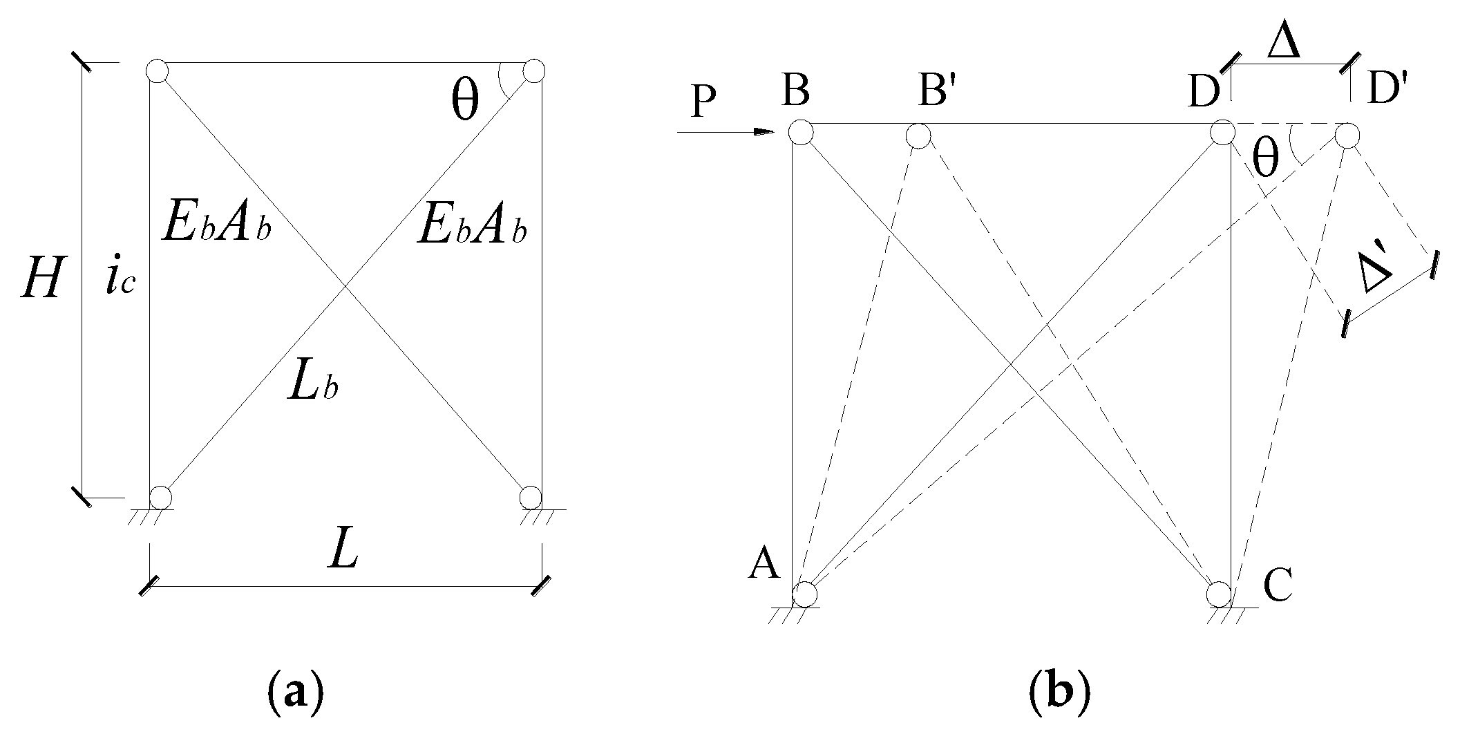
3.1.3. Determination of Elastic Lateral Stiffness Ke and Shear Capacity Fp

1. Determination of elastic lateral stiffness Ke
A simplified method for calculating the elastic lateral stiffness of the wall sheathed with double-layer wallboards on both sides was proposed by the Ye et al. [20] based on the equivalent-bracing model. The method, which avoids the high cost and time-consuming shortcomings of full-scale shear wall tests, can predict elastic lateral stiffness accurately according to sheathing material, sheathing thickness, and the shear performance of screw connections only. Consequently, this method was followed to calculate the elastic lateral stiffness of the wall with reinforced end studs. As shown in Figure 5, the simplified model is based on the following assumptions: (1) the end studs and top track are simplified as rigid bars, and the end studs are hinged to the track on the top; additionally, the bases of the end studs are assumed to be fixed ends in consideration of hold-downs; (2) the coupling of the wallboards and interior studs is equivalent to diagonal braces considering axial force only, and the equivalent braces are assumed to be the primary components for resisting lateral load; (3) the axial stiffness of the braces are cumulative.
The elastic lateral stiffness of the wall with reinforced end studs can be deduced on the basis of the above assumptions, elastic theories, structural mechanics theories, and force-balance principles, as expressed in Equation (3). The detailed derivation is described in the study by Ye et al. [20].
K e = P Δ = 6 i c H 2 + 2 L 2 i = 1 2 E b i A b i ( L 2 + H 2 ) 1.5
E b i A b i = 1 2 ( H 2 + L 2 ) 1.5 H L G i t i + 2 d e i f i n se ( H 2 + H L )
S a = H + L 2 n s + n e 5
n se = H S a + 1
where, Ke is the elastic lateral stiffness of the wall; P is lateral load; Δ is lateral displacement of the wall; ic is line rigidity of end studs; H is wall height; L is wall length; EbiAbi is axial stiffness of the brace, which is simplified from the i-layer wallboards on one side of the wall and can be determined by Equation (4); Gi and ti are shear modulus and thickness of the i-layer wallboard, respectively; fi and dei are shear strength and elastic deformation of the screw connection corresponding to the i-layer wallboard, respectively; during the calculation of EbiAbi, due to the arrangement of double-row screws for the end stud and single-line screws for the track, as shown in Figure 1, in which ns and ne are screw numbers along the vertical and horizontal edges on one side of the wall, respectively, an average space Sa of those screw connections in the perimeter of the wall was calculated first by Equation (5), and then an equivalent number nse of those screws on either the left or right side of the wall was determined according to Equation (6).
2. Determination of shear capacity Fp
Numerous experimental results show that shear capacity of CFS shear walls depends on the shear strength of the screw connections in the perimeter of the wall. The elastic model, which is usually used to determine the shear capacity of CFS shear wall [24], is not suitable for a wall with reinforced end studs. It can be explained in that the elastic model takes the load that screw connections on four corners of the wall experience as they reach their ultimate shear strength as the wall’s shear capacity, the rest of the screw connections on the end studs do not reach their ultimate strength because their horizontal force components are defined by linear conversion according to the four screw connections’ shear strength, and the failure mode of all screws on the end studs being sheared off thereby cannot be reflected during cyclic loading, resulting in lower calculated results. It also can be concluded from Table 1 that the calculated results based on the elastic model are generally 20%–35% lower than the corresponding test results.
Compared to the strip model [25] for steel plate shear walls, it can be concluded that screw connections in the perimeter of CFS shear walls can be taken as the end fields of the equivalent strips. Consequently, in considering the strip model, a simplified calculation model for the wall with reinforced end studs in shear, as shown in Figure 6, was established and based on following assumptions: (1) a wall’s shear capacity depends on the shear strength of the screw connections in the perimeter of the wall, while the screw connections in the interior studs only act as stiffeners of wallboards; (2) wallboards are divided into a series of isoclinic strips along wall length with an average space of Sa (see Equation(5)), and these strips fail only in the end fields; (3) when the screw connections in the perimeter of the walls reach their ultimate shear strength, screw holes become loose, and the strips can thereby become pinned at both ends due to the free rotation of the screws; (4) the strips can transform tension only, whose direction is the same as the wall’s diagonal direction.
The simplified calculation model, as shown in Figure 6, indicates that the shear capacity of the wall with reinforced end studs is equal to the cumulative horizontal force components of the screw connections in the perimeter of the wall. As a result of the offset horizontal forces that become separated from the screw connections on the left and right ends, only horizontal force components of the screw connections at either the top or bottom edges of the wall will be considered in the shear capacity calculation, which is denoted as:
F p = i = 1 n ee f e x i = i = 1 n ee f e i cos θ
where nee is equivalent to the number of screws either on the top or at the bottom of the wall; f e i is the shear strength of the ith screw connection in the perimeter of the wall with reinforced end studs, whose failure modes mainly exhibit in the form of a screw being sheared off or being pulled through wallboard; the two failure modes are relative to both steel thickness ts and sheathing strength, when ts is larger or the sheathing strength is higher, the steel frame can effectively restrain screw tilt, resulting in screws being sheared off, and the shear-off strength of the screw is thereby assigned to f e i , whereas when ts is relatively small or the sheathing strength is lower, screws will be pulled through the wallboard due to their tilt and will thus further sink into the wallboard, in this case, the shear strength accumulation of the connections with screws being pulled through corresponding to each layer of wallboard is assigned to f e i ; f e x i is the horizontal force component of f e i ; cosθ is angle cosine of the strip.

3.2. Hysteretic Model of Load-Displacement Curve

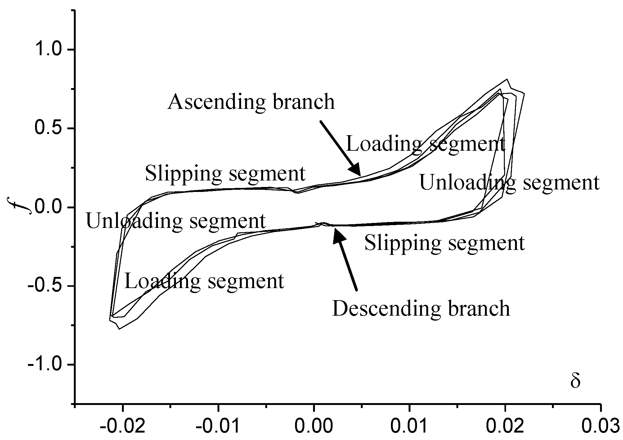
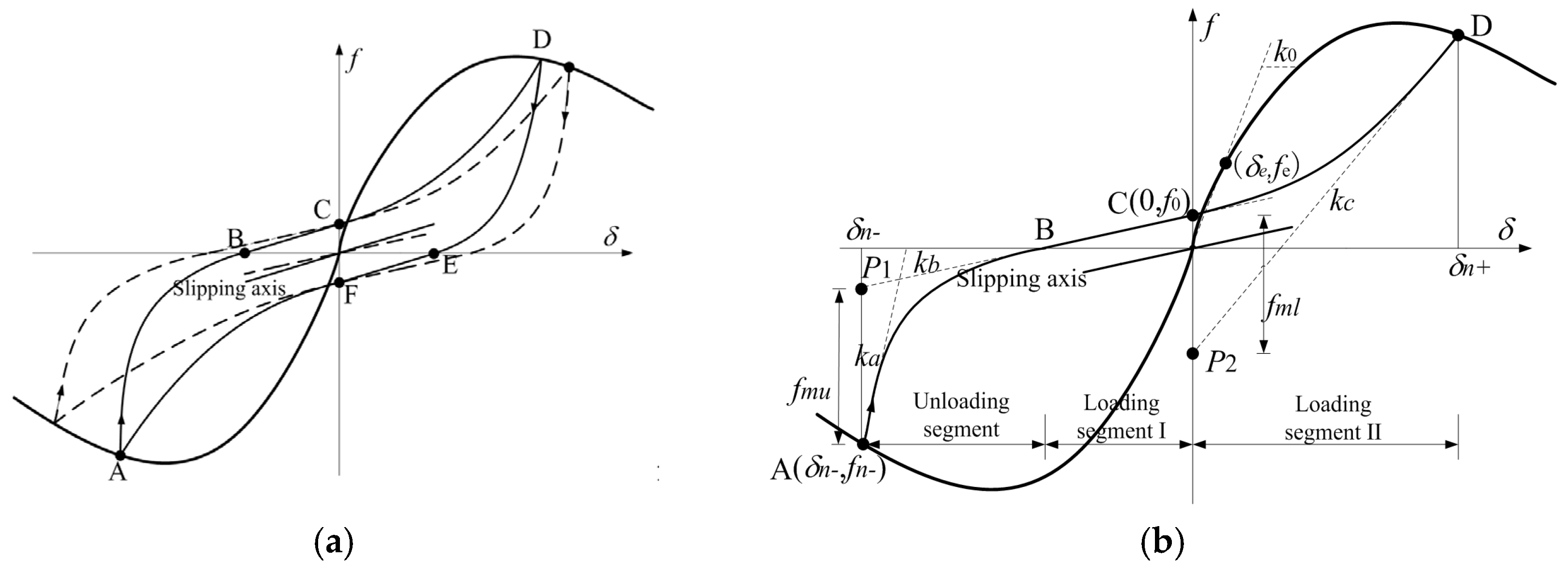
3.2.1. Model Proposition

According to previous test results, typical hysteretic loops of a wall with reinforced end studs were extracted, as shown in Figure 7, where δ is the ratio of lateral displacement Δ to wall height H; f is the ratio of lateral load F to shear capacity Fp. It can be observed that a typical hysteretic loop consists of an unloading segment, a slipping segment, and a loading segment; the ascending and descending branches of the curve are essentially symmetrical; particularly, the strength deterioration in successive cycles of the same amplitude is negligible.
Hysteretic loops for different governing deformations can be captured based on the above characteristics, and the f-δ hysteretic model of the wall can be further established, as depicted in Figure 8. As a means of simplification, strength deterioration in successive cycles of the same amplitude is not considered, each hysteresis loop has its unique slipping axis. In consideration of the symmetry of hysteretic loops, a mathematical model for the ascending branch of the curve is proposed first (see Figure 8b), and then the descending part of the curve can be obtained by origin symmetry.

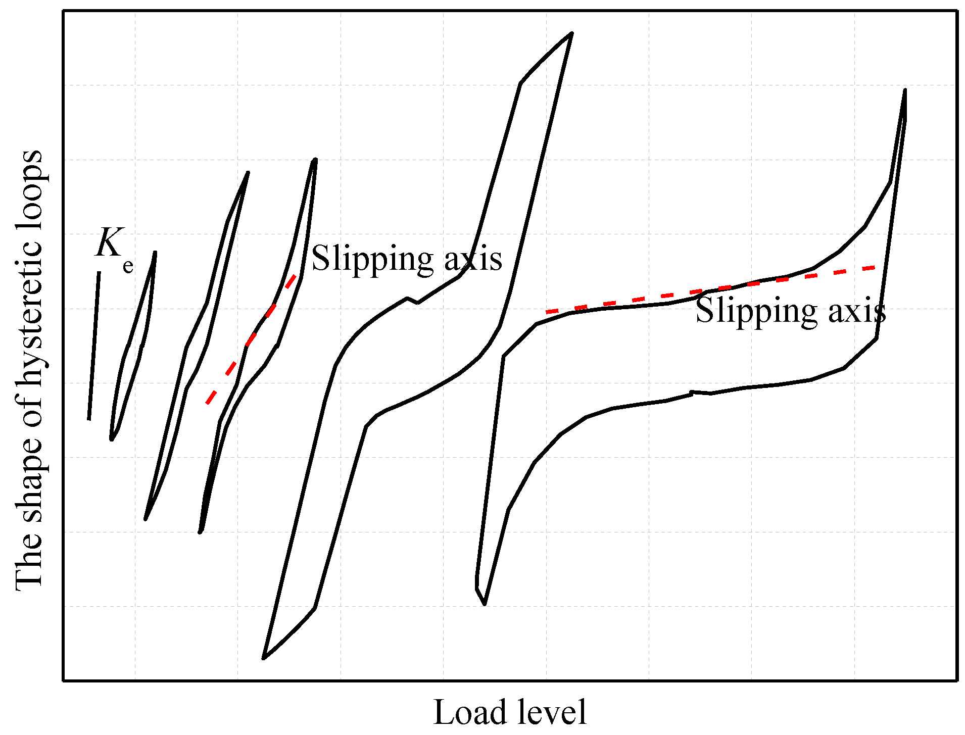
3.2.2. Modeling of Hysteretic Loop

It is difficult to describe the f-δ curve with turning points as a single equation with clear physical interpretations. Therefore, f = 0 is taken as the first demarcation point to divide the ascending branch of the curve into unloading segment AB and loading segment BCD. Furthermore, δ = 0 is taken as the second demarcation point to divide the loading segment BCD into loading segment I and loading segment II (see Figure 8b). Consequently, the ascending branch of the typical hysteretic loop consists of three segments with monotonic stiffness development, namely, the unloading segment, loading segment I, and loading segment II, where loading segment I (i.e., the slipping segment) is described linearly, because its stiffness can be seen as a constant, and the unloading segment and loading segment II are described using Richard-Abbott expressions [26]. In summary, the ascending branch of a typical hysteretic loop can be captured using the following piecewise function:
Unloading segment :   f = ( k a k b ) ( δ δ n ) [ 1 + | ( k a k b ) ( δ δ n ) f mu | n u ] 1 n u + k b ( δ δ n ) ,   f 0
Loading segment I :   f =   k b δ + f 0 ,   0 < f f 0
Loading segment II :   f = f 0 + ( k b k c ) δ [ 1 + | ( k b k c ) δ f ml | n l ] 1 n l + k c δ ,   f > f 0
where ka is the initial unloading stiffness at point A; kb is the asymptote slope of the unloading segment in the vicinity of point C; kc is the asymptote slope of the loading segment at point D; δn (including δn+ and δn− in opposite directions) is the governing deformation of the unloading segment at its initial point; fmu is the reference load of the unloading segment, which is the difference between fn− and the load of point P1, fml is the reference load of loading segment, which is the difference between the pinching load f0 at zero displacement point and the load of point P2, points P1 and P2 locate on the asymptotes of kb and kc, respectively; nu and nl are the shape parameters of the unloading segment and loading segment II, respectively.
Equations (8)–(10) show that the dominant parameters of the ascending branch of a typical hysteretic loop include ka, kb, kc, fmu, fml, nu, nl, and f0.

3.2.3. Criteria for the Dominate Parameters

1 Stiffness parameters ka, kb and kc
ka and kc are the stiffness of the f-δ curve in two opposite directions at each governing deformation (see Figure 8b), respectively, whose values under different load levels can be determined according to the test hysteretic loops measurement. The formulas of ka and kc can be obtained through the statistical analysis of the experimental results in the study by Wang and Ye [21], given by:
k a =   R a δ n + k a 0
k c =   R c 1 e R c 2 δ n + R c 3 e R c 4 δ n
where Ra is the gradient of ka with governing deformation δn; ka0 is the value of ka at δn = 0; Rc1 and Rc3 are the controlling coefficients of kc; Rc2 and Rc4 are the index gradients of kc with δn.
It can be observed form Figure 8b that kb approximates the slipping segment slope of the hysteresis loop. Therefore, the development process of those hysteretic loops obtained from previous experiments is listed in Figure 9 in order to investigate the developing rule of the slipping segment slope. It is indicated that during the initiation of the loading process, the wall is in elasticity, the curve is linear, and the slipping segment slope is equal to the elastic lateral stiffness of the wall; when the load increased, screw connections fail progressively, pinching appears in the curve because of the opening and closing of the screw holes, and the slipping segment slope decreases continuously; after an even larger amount of wall displacement, an aggravated extrusion deformation of screw connections appears, the loose screw holes cause the appearance of some no-load slipping of the screw connections, which leads the slipping axis to have a tendency towards a horizontal configuration. It can be concluded that the developing rule of the slipping segment slope is governed by a process whereby the elastic lateral stiffness of the wall decreases to a minimum value.
Based on the assumption of a linear relationship between the slipping segment slope and load level, kb can be determined:
k b =   ( 1 χ ) k 1
k 1 =   ( 1 λ ) k 0
where k1 is the difference of the slipping segment slopes between elastic and destruction phrases; k0 is the slipping segment slope in elastic phrase, which is assigned with the elastic stiffness of f-δ curve (i.e., the ratio of fe to δe that corresponds to the elastic strength limit Fe, see Figure 8b); λ is the coefficient relative to the slipping segment slope in the destruction phrase, which approximates to 0.1, according to the statistical analysis of experimental results; χ = Ci/C, in which Ci = (δnmin − 1), C = (δnmaxmin − 1), and δnmax and δmin are the maximum governing deformation and the minimum load level difference, respectively.
2 Pinching load f0
As shown in Figure 2, for each hysteretic loop, the reverse loading paths approximately direct to certain points, like pinching points C and F in Figure 8a. Screws are in the no-load slipping phrase before those pinching points are reached, at that moment, the wallboard has the least restraint on the steel frame, and the shear capacity of the frame can thereby be taken as the pinching load (approximately). Pinching load f0 is a direct reflection of the pinching characteristics of the curve. Based on a statistical analysis, a reliable constant 0.11 is assigned to f0 due to the pinching load of each specimen fluctuating around that value, which is consistent with the shear capacity of the steel frames that were tested by the authors.
3 Reference loads fmu and fml
As shown in Figure 8b, given kb, kc, and f0, the coordinates of points P1 and P2 for different governing deformations can be calculated, and the reference load fmu of unloading segment can be determined by subtracting the load of point P1 from the initial load fn− that corresponding to each governing deformation; while the reference load fml of loading segment II can be determined by subtracting the pinching load f0 from the load of P2 that corresponds to each governing deformation.
4 Shape parameters nu and nl
Through extracting nu and nl from the hysteretic curves under different load levels in the study by Wang and Ye [21], it can be concluded that nu and nl are approximately linear relative to governing deformations. The regression formulas are thereby given by:
n u =   R nu δ n + n u 0
n l =   R n l δ n + n l 0
where Rnu and Rnl are the gradients of nu (i.e., the shape parameter of unloading segment) and nl (i.e., the shape parameter of loading segment II) with governing deformation δn, respectively; nu0 and nl0 are the values of nu and nl at δn = 0, respectively.

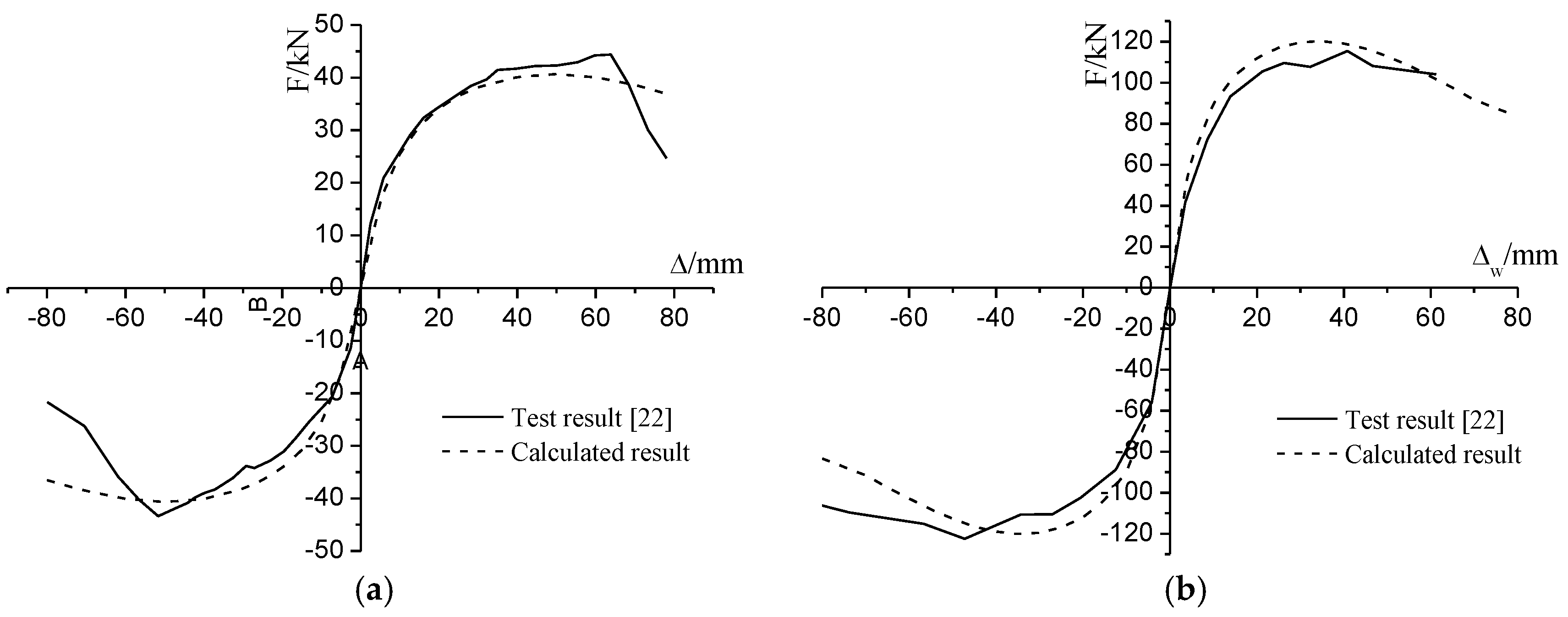
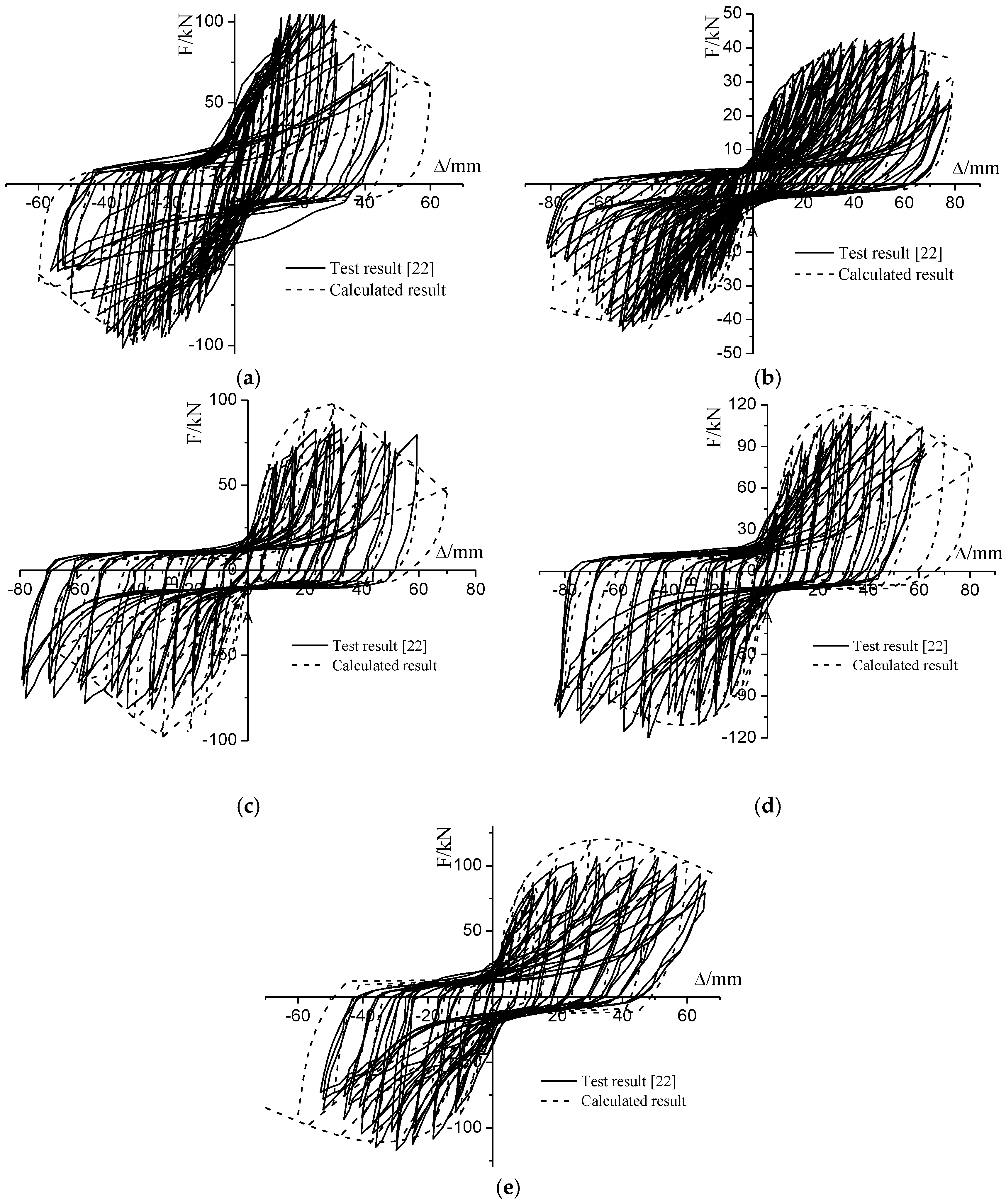
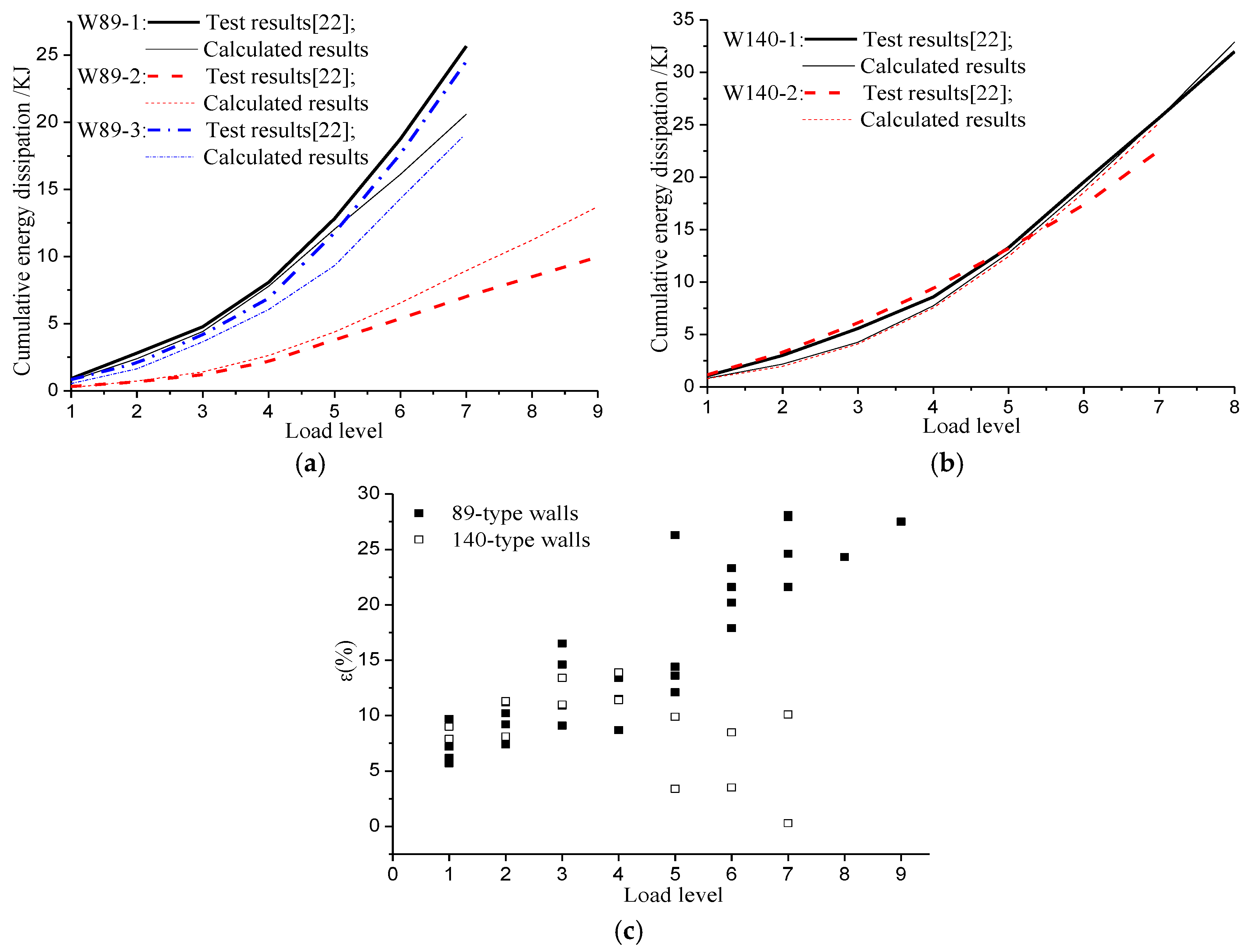
3.3. Model Verification

In order to verify the proposed hysteretic model, comparative analysis on the experimental results of the CFS shear walls described by Xu [22] was carried out, where the end stud sections of specimens include square-89 × 100 × 0.9 and square-140 × 140 × 1.5 (hereinafter referred to as 89-type and 140-type walls, respectively); all specimens were sheathed with gypsum wallboards combined with bolivian magnesium boards on both sides, whose shear modulus are 484 and 124 N/mm2, respectively; the shear performance of screw connections was determined according to the test results of Ye et al. [27], as detailed listed in Table 2.
Firstly, the elastic lateral stiffness Ke and shear capacity Fp of each specimen was determined according to the simplified method that was described in Section 3.1.3; on this basis, the discrete coordinate method was used to establish the load-displacement skeleton curves of those specimens. Limited to space, only the calculated curves of typical 89-type and 140-type walls were depicted in Figure 10. It can be observed that the calculated results, which agree well with the test results, can reflect the shear behavior of the wall with reinforced end studs like nonlinearity, stiffness, and strength deterioration. It also can be concluded from Table 3 that the calculated and test results are of high consistency in both elastic stiffness Ke and shear capacity Fp, with errors being within 11% and 15%, respectively.
Secondly, a piecewise function was adopted to establish the hysteretic loop relative to each governing deformation, and the hysteretic model of a wall was further established. Taking specimen W89-1, for example, details are as follows: (1) dimensionless treatment was performed on the load-displacement skeleton curve that was determined by the discrete coordinate method, δn and its corresponding load fn of the hysteretic loop were determined based on the load case relative to each governing deformation, and the slipping segment slope k0 in elastic phrase was calculated (see Figure 8b); (2) on the basis of k0, δn, and fn, the dominant parameters of the hysteretic model were obtained by Equations (11)–(16), as listed in Table 4, the controlling factors of parameters ka, kc, and nu, nl are listed in Table 5; (3) after substituting those dominant parameters that are listed in Table 4 into Equations (8)–(10), the f-δ hysteretic loops corresponding to different governing deformations were established, and the hysteretic model of the wall was further obtained through substituting wall height H and the calculated result of shear capacity Fpc into those f-δ loops.
Comparisons of the hysteretic curves between the calculated results and the test results are shown in Figure 11. Good agreement is observed between the test results and the calculated results, which fully reflect the hysteretic characteristics of the walls during cyclic loading.
Energy dissipation is an important indicator to measure the seismic performance of a structure or a component. The proposed hysteretic model was thereby validated by comparing the energy dissipation of the walls. Only the energy dissipation relative to the first cycle of each load level was considered, because strength deterioration in successive cycles of the same amplitude was not involved in the model.
A comparison of the cumulative energy dissipation between the calculated results and test results for each specimen is shown in Figure 12. It can be observed that during each level of horizontal load, the calculated results of the cumulative energy dissipation for 140-type walls (specimens W140-1 and W140-2) are very close to their test results; for 89-type walls, the relative errors ε of the cumulative energy dissipation between the calculated results and the test results are small in the initiation of loading and increase constantly with growing load (see Figure 12a,c). It also can be concluded from Table 3 that the relative error κ3 of the total energy dissipation between calculated results and test results for 140-type walls is within 10%, which is obviously lower than that of 89-type walls with a maximum value of 28%. The reason is that the energy dissipating mechanism of a CFS shear wall depends on the deformation of screw connections; due to a larger stiffness of the reinforced end studs in a 140-type wall, the lateral of deformation of the wall was effectively mitigated, and the deformation of the screw connections in the fields of the wall were allowed to get full development, reaping the benefit of a steady growth of the cumulative energy dissipation, therefore, the energy dissipation displayed minor differences between the calculated results and the test results during the loading process; whereas, for a 89-type wall with reinforced end studs that had lower stiffness, besides steel frame buckling, the addition of a supplementary torsional deformation, that—except for shear deformations in screw connections, which were caused by the in-plane rotation of wallboards—was involved in energy dissipation, improved the energy dissipating capacity of the wall during the later stage of loading; however, the proposed hysteretic model cannot consider both steel frame buckling and the supplementary torsional deformation into the energy dissipation of the wall, and the calculated results are thereby obviously lower than the test results.
It should be noted that, in the end of the loading process, due to a larger aspect ratio (H/L = 2.5), there was no obvious damage in specimen W89-2 except screws in the end studs being sheared off on a single side of the wall [22]. The wall’s energy dissipating capacity was significantly reduced by the insufficient deformation of screw connections (see Figure 12a). Consequently, for such walls with larger aspect ratio, the energy dissipating capacity should not be considered.

4. Summary and Conclusions

A theoretical hysteretic model, which is concise enough to be mathematically described and can reflect the shear behavior of the wall with reinforced end studs, was proposed. A degradation coefficient of secant stiffness was first introduced, and a discrete coordinate method was proposed to establish the load-displacement skeleton curve of the wall; on this basis, a piecewise function was adopted to capture the hysteretic loop relative to each governing deformation, the hysteretic model of the wall was further established, and the criteria for the dominant parameters of the model was stated. Finally, the hysteretic model was validated by the experimental results of Xu [22]. The conclusions drawn are as follows:
(1)
Elastic lateral stiffness Ke and shear capacity Fp are key factors determining the load-displacement skeleton curve of a CFS shear wall; where Ke and Fp can be predicted by the equivalent-bracing model and the proposed simplified calculation model, respectively, and the relative errors between their predicted and test results are within 11% and 15%, respectively.
(2)
The load-displacement skeleton curves determined by the discrete coordinate method agree well with the test results, which fully reflect the shear behavior (e.g., nonlinearity, stiffness, and strength deterioration) of the walls with reinforced end studs l.
(3)
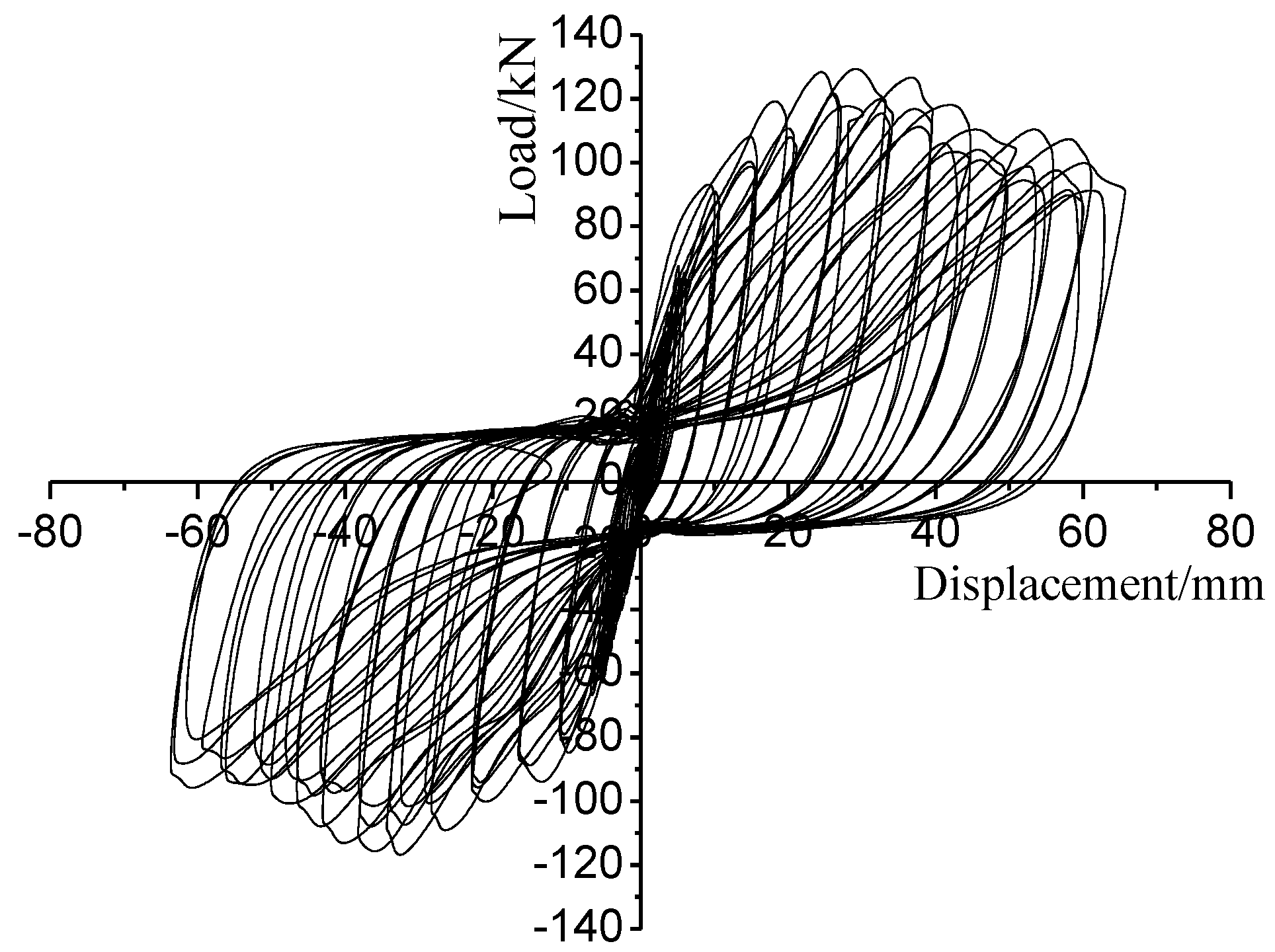
During cyclic loading, test hysteretic curves and the calculated results that were determined by the proposed hysteretic model are of high consistency in both the pinching characteristic and energy dissipating level of the walls. Due to a larger stiffness of the reinforced end studs, the relative error of the total energy dissipation between calculated and test results for 140-type walls is within 10%; whereas, for 89-type walls with reinforced end studs having lower stiffness, both steel frame buckling and a supplementary torsional deformation in screw connections were involved in energy dissipation, resulting in the calculated results being lower than the test results during the later stage of loading.
(4)
Several hysteretic models (e.g., Pinching4 material in OpenSees, BWBN model, EPHM, Pivot model, as well as the three-segment nonlinear pinching hysteretic model), were able to reproduce the behavior of the traditional shear wall with coupled C section end studs; in contrast, the proposed piecewise function hysteretic model is suitable for the wall with reinforced end studs (i.e., continuous concrete-filled rectangular steel tube columns), which is more in line with the requirements of mid-rise CFS structures, and the model has intuitional expressions with clear physical interpretations for each parameter.
(5)
Due to the significant reduction in cumulative energy dissipation that is caused by insufficient deformation of screw connections, the energy dissipating capacity of a CFS shear wall with reinforced end studs should not be considered when the wall’s aspect ratio is larger (in this study, H/L = 2.5, where H and L are wall height and wall length, respectively).

Acknowledgments

The work described in this paper was fully supported by the National Key Program Foundation of China (51538002).

Author Contributions

Jihong Ye and Xingxing Wang conceived and designed the experiments; Xingxing Wang performed the experiments; Jihong Ye and Xingxing Wang analyzed the data; Jihong Ye and Xingxing Wang wrote the paper.

Conflicts of Interest

The authors declare no conflict of interest.

References

  1. Pan, C.L.; Shan, M.Y. Monotonic shear tests of cold-formed steel wall frames with sheathing. Thin-Walled Struct. 2011, 49, 363–370. [Google Scholar] [CrossRef]
  2. Baran, E.; Alica, C. Behavior of cold-formed steel wall panels under monotonic horizontal loading. J. Constr. Steel Res. 2012, 79, 1–8. [Google Scholar] [CrossRef]
  3. Lin, S.H.; Pan, C.L.; Hsu, W.T. Monotonic and cyclic loading tests for cold-formed steel wall frames sheathed with calcium silicate board. Thin-Walled Struct. 2014, 74, 49–58. [Google Scholar] [CrossRef]
  4. Zeynalian, M.; Ronagh, H.R. Seismic performance of cold formed steel walls sheathed by fibre-cement board panels. J. Constr. Steel Res. 2015, 107, 1–11. [Google Scholar] [CrossRef]
  5. Accorti, M.; Baldassino, N.; Zandonini, R.; Scavazza, F.; Rogers, C.A. Response of CFS sheathed shear walls. Structures 2016, 7, 100–112. [Google Scholar] [CrossRef]
  6. Gad, E.F.; Chandler, A.M.; Duffield, C.F.; Stark, G. Lateral behavior of plasterboard-clad residential steel frames. J. Struct. Eng. 1999, 125, 32–39. [Google Scholar] [CrossRef]
  7. Lange, J.; Naujoks, B. Behaviour of cold-formed steel shear walls under horizontal and vertical loads. Thin-Walled Struct. 2006, 44, 1214–1222. [Google Scholar] [CrossRef]
  8. Mohebbi, S.; Mirghaderi, S.R.; Farahbod, F.; Sabbagh, A.B.; Torabian, S. Experiments on seismic behaviour of steel sheathed cold-formed steel shear walls cladded by gypsum and fiber cement boards. Thin-Walled Struct. 2016, 104, 238–247. [Google Scholar] [CrossRef]
  9. Fiorino, L.; Iuorio, O.; Macillo, V.; Landolfo, R. Performance-based design of sheathed CFS buildings in seismic area. Thin-Walled Struct. 2012, 61, 248–257. [Google Scholar] [CrossRef]
  10. Kechidi, S.; Bourahla, N. Deteriorating hysteresis model for cold-formed steel shear wall panel based on its physical and mechanical characteristics. Thin-Walled Struct. 2016, 98, 421–430. [Google Scholar] [CrossRef]
  11. Kim, T.; Wilcoski, J.; Foutch, D.A. Analysis of measured and calculated response of a cold-formed steel shear panel. J. Earthq. Eng. 2007, 11, 67–85. [Google Scholar] [CrossRef]
  12. Shamim, I.; Rogers, C.A. Steel sheathed CFS framed shear walls under dynamic loading: Numerical modelling and calibration. Thin-Walled Struct. 2013, 71, 57–71. [Google Scholar] [CrossRef]
  13. Shamim, I.; Rogers, C.A. Numerical evaluation: AISI s400 steel-sheathed CFS framed shear wall seismic design method. Thin-Walled Struct. 2015, 95, 48–59. [Google Scholar] [CrossRef]
  14. Zeynalian, M.; Ronagh, H.R. A numerical study on seismic performance of strap-braced cold-formed steel shear walls. Thin-Walled Struct. 2012, 60, 229–238. [Google Scholar] [CrossRef]
  15. Foliente, G.C. Hysteresis modeling of wood joints and structural systems. J. Struct. Eng. 1995, 121, 1013–1022. [Google Scholar] [CrossRef]
  16. Nithyadharan, M.; Kalyanaraman, V. Modelling hysteretic behaviour of cold-formed steel wall panels. Eng. Struct. 2013, 46, 643–652. [Google Scholar] [CrossRef]
  17. Pang, W.C.; Rosowsky, D.V.; Pei, S.; Van de Lindt, J.W. Evolutionary parameter hysteretic model for wood shear walls. J. Struct. Eng. 2007, 133, 1118–1129. [Google Scholar] [CrossRef]
  18. Huang, Z.G.; Wang, Y.J.; Su, M.Z.; Shen, L. Study on restoring force model of cold-formed steel wall panels and simplified seismic response analysis method of residential buildings. China Civ. Eng. J. 2012, 45, 26–34. [Google Scholar]
  19. Zhou, X.H.; Yuan, X.L.; Shi, Y.; Nie, S.F.; Zhao, H.J. Research on nonlinear pinching hysteresis model of sheathed cold-formed thin-walled steel stud walls. Eng. Mech. 2012, 29, 224–233. [Google Scholar]
  20. Ye, J.H.; Wang, X.X.; Jia, H.Y.; Zhao, M.Y. Cyclic performance of cold-formed steel shear walls sheathed with double-layer wallboards on both sides. Thin-Walled Struct. 2015, 92, 146–159. [Google Scholar] [CrossRef]
  21. Wang, X.X.; Ye, J.H. Reversed cyclic performance of cold-formed steel shear walls with reinforced end studs. J. Constr. Steel Res. 2015, 113, 28–42. [Google Scholar] [CrossRef]
  22. Xu, Y. Experimental Research on Shear Performance of New-type Cold-Formed Steel Load Bearing Walls; Southeast University: Nanjing, China, 2016. (In Chinese) [Google Scholar]
  23. Tian, H.W.; Li, Y.Q.; Cheng, Y. Testing of steel sheathed cold-formed steel trussed shear walls. Thin-Walled Struct. 2015, 94, 280–292. [Google Scholar] [CrossRef]
  24. Chen, C.Y.; Okasha, A.F.; Rogers, C.A. Analytical predictions of strength and deflection of light gauge steel frame/wood panel shear walls. In Proceedings of the International Conference on Advances in Engineering Structures, Mechanics & Construction, Waterloo, ON, Canada, 14–17 May 2006; pp. 381–391.
  25. Shao, J.H.; Gu, Q.; Shen, Y.K. Analysis of elastic-plastic shear resistance for steel plate shear walls. J. Hohai Univ. (Nat. Sci.) 2006, 34, 537–541. [Google Scholar]
  26. Fiorino, L.; Iuorio, O.; Landolfo, R. Seismic analysis of sheathing-braced cold-formed steel structures. Eng. Struct. 2012, 34, 538–547. [Google Scholar] [CrossRef]
  27. Ye, J.H.; Wang, X.X.; Zhao, M.Y. Experimental study of shear behavior of screw connections in CFS sheathing. J. Constr. Steel Res. 2016, 121, 1–12. [Google Scholar] [CrossRef]
Figure 1. Construction of a cold-formed steel (CFS) shear wall with reinforced end studs. CFRST, concrete-filled rectangular steel tube.
Applsci 07 00094 g001
Figure 2. Typical load-displacement hysteretic curve. Reprinted from [21]. Copyright 2015, with permission from Elsevier.
Applsci 07 00094 g002
Figure 3. Degradation trends of secant stiffness.
Applsci 07 00094 g003
Figure 4. Discrete coordinate method.
Applsci 07 00094 g004
Figure 5. Equivalent-bracing model. (a) Simplification model; (b) calculation model. Reprinted from [20]. Copyright 2015, with permission from Elsevier.
Applsci 07 00094 g005
Figure 6. Simplified calculation model for the wall with reinforced end studs in shear.
Applsci 07 00094 g006
Figure 7. Typical hysteretic loops.
Applsci 07 00094 g007
Figure 8. Hysteretic model of a wall with reinforced end studs. (a) Hysteretic laws; (b) calculation model for the ascending branch of the curve. Note: The symbols’ meanings are identical to those in Equations (8)–(16).
Applsci 07 00094 g008
Figure 9. Development process of the hysteretic loops of the wall.
Applsci 07 00094 g009
Figure 10. Comparisons of the load-displacement skeleton curves of typical specimens. (a) 89-type wall (specimen W89-2); (b) 140-type wall (specimen W140-1).
Applsci 07 00094 g010
Figure 11. Hysteretic curves of test results and the proposed hysteretic model. (a) Specimen W89-1; (b) Specimen W89-2; (c) Specimen W89-3; (d) Specimen W140-1; (e) Specimen W140-2.
Applsci 07 00094 g011
Figure 12. Cumulative energy dissipation of test and the proposed hysteretic model. (a) 89-type walls; (b) 140-type walls; (c) Relative errors ε between calculated and test results.
Applsci 07 00094 g012
Table 1. Comparison of the shear capacity Fp of the wall with reinforced end studs.
Specimen Number [21]Test Results/kNCalculated Results Based on Elastic Model/kNRelative Errors
WA1100.079.7−20.3%
WA2101.581.4−19.8%
WA3109.081.4−25.3%
WB1126.5101.5−19.8%
WB260.345.3−24.9%
WC1109.870.6−35.7%
WC295.470.6−26.0%
WC367.045.3−32.4%
Table 2. The shear performance of screw connections [27] 1.
Failure ModesSteel Thickness (mm)12 mm Gypsum Wallboard12 mm Bolivian Magnesium Boardfe/kN
de/mmf/kNde/mmf/kN
Screw being pulled through0.90.700.660.630.741.40
1.20.620.730.500.701.43
Screw being sheared off-----1.78
1 f and de are the shear strength and elastic deformation of a screw connection sheathed with a single-layer wallboard, respectively; fe is the shear strength of a screw connection in the perimeter of the wall with reinforced end studs.
Table 3. Comparisons between the calculated and test results 1.
Specimen Number [22]Wall Size/m (L × H)Elastic Lateral Stiffness Ke (N/mm)Shear Capacity Fp/kNTotal Energy Dissipation E/KJ
KetKecκ1FptFpcκ2EtEcκ3
W89-13.6 × 3.09670101770.05110.298.0−0.1125.720.60.25
W89-21.2 × 3.034883400−0.0244.440.6−0.0810.013.70.27
W89-33.6 × 3.09192101770.1185.498.00.1524.519.20.28
W140-13.6 × 3.01208511573−0.04122.6120.0−0.0232.032.90.03
W140-23.6 × 3.01222711573−0.05117.2120.00.0222.625.20.10
1 Ket and Kec are the test and calculated results of elastic lateral stiffness, respectively; Fpt and Fpc are the test and calculated results of shear capacity, respectively; Et and Ec are the test and calculated results of total energy dissipation, respectively; κ1, κ2, and κ3 are the relative errors between Ket and Kec, Fpt, and Fpc, and Et and Ec, respectively.
Table 4. The dominant parameters used to the hysteretic model of specimen W89-1 1.
Load Caseδnfnk0kakbkcfmufmlnunlf0
10 mm0.00330.847125.0788.4102.3502.41.0741.2581.451.350.11
15 mm0.0050.948125.0827.392.0285.61.2981.0501.401.400.11
20 mm0.00670.998125.0866.281.8206.21.4361.0411.351.460.11
30 mm0.011.0125.0941.861.4148.81.5041.2121.251.570.11
40 mm0.01330.916125.01017.340.9118.71.3501.3171.151.680.11
50 mm0.01670.791125.01095.120.495.41.0221.2521.041.780.11
60 mm0.020.657125.01170.712.577.20.7971.2470.941.890.11
1 k0 is the slipping segment slope of the wall in elasticity (see Figure 8b); the rest of the symbols’ meanings are identical to those in Equations (8)–(10).
Table 5. The controlling factors of parameters ka, kc, and nu, nl 1.
Raka0Rc1Rc2Rc3Rc4RnuRnlnu0nl0
22892.0712.82813.4−701.4277.0−63.930.232.51.551.24
1 The meaning of each symbol is identical to the definitions provided in Equations (11)–(16).

