A Novel Adaptive PID Controller with Application to Vibration Control of a Semi-Active Vehicle Seat Suspension

Abstract

This work proposes a novel adaptive hybrid controller based on the sliding mode controller and H-infinity control technique, and its effectiveness is verified by implementing it in vibration control of a vehicle seat suspension featuring a magneto-rheological damper. As a first step, a sliding surface of the sliding mode controller is established and used as a bridge to formulate the proposed controller. In this process, two matrices such as Hurwitz constants matrix are used as components of the sliding surface and H-infinity technique are adopted to achieve robust stability. Secondly, a fuzzy logic model based on the interval type 2 fuzzy model which is featured by online clustering is established and integrated to take account for external disturbances. Subsequently, a new adaptive hybrid controller is formulated with a solid proof of the robust stability. Then, the effectiveness is demonstrated by implementing the proposed hybrid controller on the vibration control of a vehicle seat suspension associated with a controllable damper. Vibration control performances are evaluated on bump and random road profiles by presenting both displacement and acceleration on the seat and the driver positions. In addition, a comparative study between the proposed and one of existing controllers is undertaken to highlight some benefits of the hybrid adaptive controller developed in this work.

1. Introduction

Recently, many studies on the formulation of various hybrid control schemes using classical/modern controllers and intelligent control techniques have been undertaken. In the formulation of the hybrid controllers, PID (proportional-integral-derivative) controller, LQG (linear quadratic Gaussian) optimal controller, H-infinity controller, and sliding mode controller are frequently adopted as a classical/modern controller, while the fuzzy logic controller, neural network controller, and neural network-fuzzy controller are often used as intelligent controllers. One of main reasons to develop hybrid controllers is to enhance control performance as well as achieve control robustness against parameter variations and external disturbances. In addition, during realization of the hybrid controllers, the salient features of each controller are kept and hence one can achieve more precise and better control performance than the use of a single controller only. Therefore, in general, the hybrid controller is well suitable to many dynamic systems subjected to uncertainties and disturbances. For the last decade, among intelligent controllers the fuzzy control method is most frequently used to formulate a new hybrid controller. Normally, the fuzzy control method is divided into two types; type 1 fuzzy model and interval type 2 fuzzy model. A hybrid adaptive fuzzy controller based on H-infinity technique was presented in [1]. In this controller, adaptation laws were developed by using parameters of Riccati-like equation and non-derivative functions. To guarantee control robustness, error dynamics were proposed and combined with the laws. The H-infinity technique was also used to design a hybrid adaptive controller in [2]. The H-infinity tracking inequality function was modified following the sum of values of adaptive function at zero. The sum function was less than the prescribed value which was defined in the adaptation law. A similar hybrid controller was also proposed in [3] and the combination of the fuzzy-neural networks model and H-infinity technique was presented in [4]. In this work, the Riccati-like equation was modified, and then the modified parameters were used as a robust control function. On the other hand, a different type of hybrid controller using several control strategies such as H-infinity technique, sliding mode control, and fuzzy model were suggested in [5]. The H-infinity inequality function was modified following the sum and integration of the prescribed attenuation value, and control robustness was derived from the simplified inequality function of the Riccati-like equation. The disadvantage of this hybrid controller is slow response (or heavy calculation) because of the complicated functions. A similar hybrid controller was also presented in [6]. It should be noted here that the hybrid controllers formulated in previous studies mostly featured the type 1 fuzzy model.

A hybrid adaptive controller utilizing the interval type 2 fuzzy model was proposed in [7,8]. In these works, a hybrid controller was formulated by combining several control methodologies such as sliding mode function, H infinity technique, and the type 2 fuzzy model. In this case, adaptation laws and inequality functions should be determined considering the inherent properties of each controller. The design method of this type of hybrid controller was also described in [9,10,11,12,13]. It is noted that the recursive method for design of an adaptive controller has been introduced in [11] and the direct adaptive control method has been used to formulate a hybrid controller [8]. Another method for the design of adaptive controller is to combine the fuzzy model and H-infinity approach by considering the back-stepping method [14]. In this case, the adaptation law was a sum function of parameters of the fuzzy output and calculated factors of the back-stepping function. The model of interval type 2 fuzzy model was used and combined with a new sigmoid function of the sliding mode control to design a hybrid controller [15]. A similar adaptive fuzzy H-infinity controller was also studied by considering the linear matrix inequality approach [16]. A new hybrid controller with a special exponential function was developed by combining the fuzzy model, the sliding surface, and H-infinity technique [17]. Recently, the development of a new adaptive controller integrated with a PI controller was also undertaken [18]. It is noted here that, in order to develop an effective hybrid controller, the property of uncertain (indefinite) systems should be removed. One of solutions is to use the interval type 2 fuzzy (IT2F in short) model. However, prior to applying the IT2F, the clustering method for finding the feature of the uncertain system needs to be clearly expressed [19,20,21]. Basic theory and mathematical algorithm for IT2F should especially be analyzed in detail [22,23,24,25,26,27,28,29,30]. In these references, the calculation of the centroid and fast algorithm for the output of the fuzzy variables have been well described to improve the IT2F model. As surveyed from above literature, the design freedom to formulate new hybrid controllers which can significantly enhance control performance compared with the use of single controller is limitless. It is vital that an advanced hybrid controller needs to be developed for control systems subjected to uncertainties and external disturbances to guarantee robust and high control performance.

Consequently, the main technical contributions of this work can be summarized as follows: (i) the design of new hybrid controller whose structure is relatively simple compared with existing hybrid controller; (ii) the proof of robust stability of the proposed hybrid controller consisting of the H-infinity control and sliding mode control methods based on the type 2 fuzzy model; and (iii) the experimental verification of enhanced robust control performances with an application to a semi-active vehicle seat suspension system subjected to parameter uncertainties and road disturbances.

In order to accomplish these contributions, the design concept to formulate a new hybrid controller is chosen as two aspects; simple structure and excellent control performances in the presence of both the uncertainties and external disturbances. Therefore, as a first step, a new hybrid controller is formulated by adopting the H-infinity control and sliding mode control methods based on the type 2 fuzzy model. Then, the stability of control system is solidly proven through Lyapunov stability criterion. Subsequently, in order to demonstrate some benefits of the proposed hybrid controller, a seat suspension system for commercial bus which is controlled by a magneto-rheological (MR) damper (MR seat suspension system in short) is established. Both computer simulation and experimental results such as acceleration on the seat position are presented in the time domain. In addition, the results obtained from the proposed hybrid controller are compared with the results achieved from the hybrid controller developed in [5] showing displacement and acceleration on the seat and driver. It is noted that the hybrid controller developed in [5] is adopted as a comparative one since this hybrid controller combines same control strategies of H-infinity control, fuzzy logic, and sliding mode control, as those used for the hybrid controller proposed in this current work.

2. New Adaptive Hybrid Controller

As mentioned above, the proposed control is established based on the fuzzy model, H infinity technique, and PID control. The combination of these controls relies on the advantages of each controller; the fuzzy model is used for the formulation of the dynamic model associated with the uncertainty, the PID controller is used to adaptively adjust control gains, and the H infinity technique connected with the PID controller is used to guarantee the robustness to uncertainties such as parameter variations and external disturbance. By combining several control algorithms, the stability of the control system subjected to heavy uncertainties can be improved and control performance can be easily tuned by adjusting control gains of each control logic.

2.1. Online Interval Type 2 Fuzzy Neural Network Model

Since the fuzzy model is used for the formulation of the dynamic model, the inherent features of the fuzzy rule are introduced before designing the control system. These features are the basis for establishing the fuzzy models of dynamic parameters. The salient points of this method are given as follows. There is no constraint of the feature in inputs and the most effective feature is determined through calculation process. In addition, from this method the fuzzy model can be exactly determined, and hence the error caused from the designer in choosing fuzzy models can be reduced. Based on the feature cluster of the granular clustering method, the initial fuzzy rules are established. These rules support the control system in the first time, and provide online fuzzy rules in the next step. The result of the granular clustering method is a part of an online interval type 2 fuzzy neural networks (OIT2FNN in short) model [18]. The output of OIT2FNN follows the Takagi–Sugeno–Kang type (TSK in short). The rule base of OIT2FNN can be expressed as [18,20]

$$R_f{}^j:\mathrm{If}{h}_1\mathrm{is}{\mathit{H}}_{f\mathbf{1}}^{\mathit{j}}\mathrm{and}\dots \mathrm{and}{h}_n\mathrm{is}{\mathit{H}}_{f\mathit{n}}^{\mathit{j}}\mathrm{then}g\mathrm{is}{a}_0^j+{\displaystyle \sum _{i=1}^n{a}_i^j}{h}_i$$

(1)

where, ${\mathit{H}}_{f\mathit{i}}^{\mathit{j}}\left(i=1,\dots ,n;j=1,\dots ,m\right)$ are fuzzy sets, $m$ is the number of rules, and $a_i^j$ are interval sets. The calculation process of OIT2FNN is clearly depicted in [17,18]. The defuzzified output is then determined by

$$g_f=\frac{g_l+g_r}{2}=\frac{{\theta }_l^T{\xi }_l^f+{\theta }_r^T{\xi }_r^f}{2}$$

(2)

In the above, ${\theta }_l^T=\left[w_1^l{w}_2^l{w}_3^l\dots w_n^l\right]$ and ${\theta }_r^T=\left[w_1^r{w}_2^r{w}_3^r\dots w_n^r\right]$ are the weighting vectors, which symbolize the relation of the rule layer and type-reduction, and the weighted firing strength vectors are given by

$${\xi }_l^f={\left[\frac{{\underset{\_}{f}}_1}{{\displaystyle \sum _{i=1}^n{\underset{\_}{f}}_i}}\frac{{\underset{\_}{f}}_2}{{\displaystyle \sum _{i=1}^n{\underset{\_}{f}}_i}}\frac{{\underset{\_}{f}}_3}{{\displaystyle \sum _{i=1}^n{\underset{\_}{f}}_i}}\dots \frac{{\underset{\_}{f}}_n}{{\displaystyle \sum _{i=1}^n{\underset{\_}{f}}_i}}\right]}^T,{\xi }_r^f={\left[\frac{{\overline{f}}_1}{{\displaystyle \sum _{i=1}^n{\overline{f}}_i}}\frac{{\overline{f}}_2}{{\displaystyle \sum _{i=1}^n{\overline{f}}_i}}\frac{{\overline{f}}_3}{{\displaystyle \sum _{i=1}^n{\overline{f}}_i}}\dots \frac{{\overline{f}}_n}{{\displaystyle \sum _{i=1}^n{\overline{f}}_i}}\right]}^T.$$

2.2. Adaptive Hybrid Control

In this study, the nth-order nonlinear system is used to define a new proposed controller. Its equation is expressed by

$$\dot{x}=f\left(x\right)+g\left(x\right)u\left(t\right)+d\left(t\right)$$

(3)

The above equation strictly follows the assumption given below.

Assumption 1. In Equation (3), the functions $f\left(x\right)\in R^n$ and $g\left(x\right)\in R^n$ are two unknown non-linear function vectors, $u\left(t\right)\in R^1$ is the control function, $d\left(t\right)\in R^n$ is the external disturbance vector, $\left|d\left(t\right)\right|\le \delta d$ where $\delta d\in R^n$ is the upper bound of $d\left(t\right)$, and $x=\left[x_1,x_2,\dots ,x_n\right]={\left[x_1,x_1,\dots ,x_1{}^{(n-1)}\right]}^T\in R^n$ is the state vector of the system.

The system (3) can be rewritten as

$$\dot{x}=f_{\mathbf{0}}(x)+g_{\mathbf{0}}(x)u\left(t\right)+D\left(t\right)$$

(4)

where, $D\left(t\right)=\delta f+\delta gu\left(t\right)+d(t)$ denotes the uncertain disturbances which can be redefined by $D={\left[0,0,\dots ,D_0\right]}^T$, $f_0\left(x\right)={\left[x_2,\dots ,x_n,f_0\right]}^T$, $g_0\left(x\right)={\left[0,\dots ,0,g_0\right]}^T$, $\delta f={\left[0,0,\dots ,\delta f_0\right]}^T$, $\delta g={\left[0,0,\dots ,\delta g_0\right]}^T$. It is noted that $\delta f$ and $\delta g$ are two positive vectors. Based on Equation (2), the relationship between system (4) and OIT2FNN is determined as

$$f_{00}\left(x\right)=f_0\left(x\right)g_f={\theta }_f{\xi }_f$$

(5)

$$g_{00}\left(x\right)=g_0\left(x\right)g_f={\theta }_g{\xi }_g$$

(6)

In the above, ${\theta }_f={\left[{\theta }_f^l,{\theta }_f^u\right]}^T$, ${\theta }_g={\left[{\theta }_g^l,{\theta }_g^u\right]}^T$ and ${\xi }_f={\xi }_g=\left[{\xi }_l,{\xi }_u\right]$. Note that ${\theta }_f,{\theta }_g$ are the centroid of consequent vectors. ${\xi }_f$,${\xi }_g$ are consequent membership vectors of $f,g$, respectively. The sliding surface $s_s$ of the sliding mode control is defined as

$$s_s=k_1{x}_1+k_2{x}_2+k_3{x}_3+\dots +k_n{x}_n={\displaystyle \sum _{i=1}^n{k}_i{x}_i}$$

(7)

where, $K=\left[k_n,k_{n-11},k_{n-2},\dots ,k_1\right]$is defined as the coefficients such that all of the roots of the polynomial ${\sigma }^n+k_{n-1}{\sigma }^{n-1}+k_{n-2}{\sigma }^{n-2}+\dots +k_1$ are in the open left-half complex plane. It is noted that $k_n=1$ in this analysis. The sliding surface in Equation (7) is rewritten using the state variables as

$$x_n=-k_1{x}_1-k_2{x}_2-k_3{x}_3-\dots -k_{n-1}{x}_{n-1}+s_s$$

(8)

A new vector $\tilde{x}$ is defined by $\tilde{x}={\left[x_1{x}_2{x}_3\dots x_{n-1}\right]}^T$, and thus the system (4) is rewritten as

$$\dot{\tilde{x}}=S_1\tilde{x}+S_2^T{s}_s$$

(9)

where,

$$S_1=\left[\begin{array}{cccc}0& 1& 0& \begin{array}{cc}\dots & 0\end{array}\\ 0& 0& 1& \begin{array}{cc}\dots & 0\end{array}\\ .& .& .& \begin{array}{cc}\dots & .\end{array}\\ -k_1& -k_2& -k_3& \begin{array}{cc}\dots & -k_{n-1}\end{array}\end{array}\right],S_2=\left[\begin{array}{c}0\\ 0\\ .\\ 1\end{array}\right]$$

The derivative of Equation (7) yields the equation

$${\dot{s}}_s=k_1{\dot{x}}_1+k_2{\dot{x}}_2+k_3{\dot{x}}_3+\dots +k_{n-1}{\dot{x}}_{n-1}+f_0(x)+g_0(x)u\left(t\right)+D\left(t\right)$$

(10)

To simplify the control, the lumped uncertainty is defined by

$$w_l={\tilde{\gamma }}_f{\xi }_f+{\tilde{\gamma }}_g{\xi }_{g}u+D$$

(11)

where, ${\tilde{\gamma }}_f=f_0\left(x\right)-f_{00}^{\ast }\left(x\right)$, ${\tilde{\gamma }}_g=g_0\left(x\right)-g_{00}^{*}\left(x\right)$. Substituting Equation (11) into Equation (10) yields the equation

$${\dot{s}}_s={\displaystyle \sum _{i=1}^{n-1}{k}_i{x}_{i+1}}+f_{00}^{*}\left(x\right)+g_{00}^{*}\left(x\right)u+w_l$$

(12)

Then, Equation (12) can be written by substituting values of OIT2FNN as

$${\dot{s}}_s={\displaystyle \sum _{i=1}^{n-1}{k}_i{x}_{i+1}}+{\theta }_f^{*}{\xi }_f+{\theta }_g^{*}{\xi }_{g}u+w_l$$

(13)

where, ${\theta }_f^{*}=\arg {\min }_{{\theta }_f\in \Delta {\theta }_f}\left[{\sup }_{x\in \Delta x}\left|f\left(x\right)-f_{00}^{}\left(x\right)\right|\right]$, ${\theta }_g^{*}=\arg {\min }_{{\theta }_g\in \Delta {\theta }_g}\left[{\sup }_{x\in \Delta x}\left|g\left(x\right)-g_{00}^{}\left(x\right)\right|\right]$, $\Delta {\theta }_f=\left\{{\theta }_f\in R^n,\Vert {\theta }_f\Vert \le {\epsilon }_f\right\}$, $\Delta {\theta }_g=\left\{{\theta }_g\in R^n,\Vert {\theta }_g\Vert \le {\epsilon }_g\right\}$, $\Delta x=\left\{x\in R^n,\Vert x\Vert \le {\epsilon }_x\right\}$.

In the above, ${\epsilon }_f,{\epsilon }_g,{\epsilon }_x$ are constant boundaries. An equivalent control of the system is derived from Equation (13) based on assumption of $w_l\approx 0$

$$u_1=-\frac{1}{{\widehat{\theta }}_g{\xi }_g}\left({\displaystyle \sum _{i=1}^{n-1}{k}_i{x}_{i+1}}+{\widehat{\theta }}_f{\xi }_f\right)$$

(14)

The equivalent control $u_1$ cannot control the system because it cannot compensate the error from the fuzzy approximation. To guarantee the robustness and stability in control, a robust control part $u_2$ should be added as

$$u_2=\frac{1}{{\widehat{\theta }}_g{\xi }_g}\left(-{\displaystyle \sum _{i=1}^{n-1}{P}_{\left(n-1\right)i}{x}_i}-\frac{s_s}{\beta }+\frac{1}{2}\Gamma s_s{\xi }_{fz}\tilde{x}P{S}_2{S}_2^{T}P{\tilde{x}}^T+K_P{s}_s{}^{2}e+K_I{s}_s{}^2{\displaystyle \int edt+K_D{s}_s{}^2\frac{de}{dt}}\right)$$

(15)

where, $e=x_d-x$ is tracking error and $x_d$ is the desired value. The control $u_2$ is the combination of the sliding surface of $s_s$, H-infinity controller and PID controller. The value $\Gamma$ is the adaptive parameter where its boundary is given by $\Delta \Gamma =\left\{\Gamma \in R,\Vert \Gamma \Vert \le {\epsilon }_{\Gamma },\Gamma {\xi }_{fz}\le \rho \right\}$, and ${\epsilon }_{\Gamma }$ is constant boundary. The matrix $P=P^T\ge 0$ in which its result is a solution of Riccati-like equation given by

$$P{S}_1+S_1^{T}P+Q-s_s\Gamma {\xi }_{fz}P{S}_2{S}_2^{T}P+\rho P{S}_2{S}_2^{T}P=0$$

(16)

Besides, the boundaries of $K_P$, $K_I$, and $K_D$ are determined as $\Delta K_P=\left\{K_P\in R,\Vert K_P\Vert \le {\epsilon }_{KP}\right\}$, $\Delta K_I=\left\{K_I\in R,\Vert K_I\Vert \le {\epsilon }_{KI}\right\}$, $\Delta K_D=\left\{K_D\in R,\Vert K_D\Vert \le {\epsilon }_{KD}\right\}$. In these boundaries, ${\epsilon }_{KP}$, ${\epsilon }_{KI}$ and ${\epsilon }_{KD}$ are constant. Finally, the control $u$ of the system is determined as

$$u=u_1+u_2$$

(17)

Remark 1. 

To evaluate the stability and robustness of the system, Lyapunov function of the system (3) is suggested as

$$V=\frac{1}{2}{s}_s{}^2+\frac{1}{2}\tilde{x}P{\tilde{x}}^T+\frac{1}{2{\eta }_1}{\tilde{\gamma }}_f^2+\frac{1}{2{\eta }_2}{\tilde{\gamma }}_g^2+\frac{1}{2{\eta }_3}{\Gamma }^2+\frac{1}{2{\eta }_4}{K}_P^2+\frac{1}{2{\eta }_5}{K}_I^2+\frac{1}{2{\eta }_6}{K}_D^2$$

(18)

Based on the evaluation, six adaptation laws are found as

$${\dot{\tilde{\gamma }}}_f=-{\eta }_1{s}_s{\xi }_p$$

(19)

$${\dot{\tilde{\gamma }}}_g=-{\eta }_2{s}_s{\xi }_q{u}_1$$

(20)

$$\dot{\Gamma }=-{\eta }_3{s}_s{\xi }_{fz}\tilde{x}P{S}_2{S}_2^{T}P{\tilde{x}}^T$$

(21)

$${\dot{K}}_P=-{\eta }_4{s}_s{}^2{\xi }_{fz}e$$

(22)

$${\dot{K}}_I=-{\eta }_5{s}_s{}^2{\xi }_{fz}{\displaystyle \int e}dt$$

(23)

$${\dot{K}}_D=-{\eta }_6{s}_s{}^2{\xi }_{fz}\frac{de}{dt}$$

(24)

Now, the adaptation laws of the proposed hybrid adaptive controller can be summarized in the following theorem.

Theorem 1. 

The adjusted adaptation laws of the proposed hybrid controller given by Equations (19)–(24) are modified to satisfy Lyapunov stability as

$${\dot{\tilde{\gamma }}}_f=\{\begin{array}{c}\begin{array}{cc}-{\eta }_1{s}_s{\xi }_f& if\Vert {\tilde{\gamma }}_{\mathrm{f}}\Vert <{\epsilon }_{f}or\left(\Vert {\tilde{\gamma }}_f\Vert ={\epsilon }_{f}and{s}_s{\xi }_f{\tilde{\gamma }}_f\ge 0\right)\end{array}\\ \begin{array}{cc}-{\eta }_1{s}_s{\xi }_f+{\eta }_1\frac{\left({\Vert {\tilde{\gamma }}_f\Vert }^2-{\epsilon }_f\right)s_s{\xi }_f{\tilde{\gamma }}_f}{{\delta }_1{\Vert {\tilde{\gamma }}_f\Vert }^2}& if\Vert {\tilde{\gamma }}_f\Vert ={\epsilon }_{f}and{s}_s{\xi }_f{\tilde{\gamma }}_f<0\end{array}\end{array}$$

(25)

$${\dot{\tilde{\gamma }}}_g=\{\begin{array}{c}\begin{array}{cc}-{\eta }_2{s}_s{\xi }_g{u}_1& if\Vert {\tilde{\gamma }}_{\mathrm{g}}\Vert <{\epsilon }_{g}or\left(\Vert {\tilde{\gamma }}_{\mathrm{g}}\Vert ={\epsilon }_{g}and{s}_s{\xi }_g{u}_1{\tilde{\gamma }}_{\mathrm{g}}\ge 0\right)\end{array}\\ \begin{array}{cc}-{\eta }_2{s}_s{\xi }_g{u}_1+{\eta }_2\frac{\left({\Vert {\tilde{\gamma }}_g\Vert }^2-{\epsilon }_g\right)s_s{\xi }_g{u}_1{\tilde{\gamma }}_g}{{\delta }_2{\Vert {\tilde{\gamma }}_g\Vert }^2}& if\Vert {\tilde{\gamma }}_{\mathrm{g}}\Vert ={\epsilon }_{g}and{s}_s{\xi }_g{u}_1{\tilde{\gamma }}_{\mathrm{g}}<0\end{array}\end{array}$$

(26)

$$\dot{\Gamma }=\{\begin{array}{c}\begin{array}{cc}-{\eta }_3{s}_s{\xi }_{fz}\tilde{x}P{S}_2{S}_2^{T}P{\tilde{x}}^T& \begin{array}{l}if\Vert \Gamma \Vert <{\epsilon }_{\Gamma }or\\ \left(\Vert \Gamma \Vert ={\epsilon }_{\Gamma }+{\delta }_{3}and{s}_s{\xi }_{fz}\tilde{x}P{S}_2{S}_2^{T}P{\tilde{x}}^T\Gamma \ge 0\right)\end{array}\end{array}\\ \begin{array}{cc}-{\eta }_3{s}_s{\xi }_{fz}\tilde{x}P{S}_2{S}_2^{T}P{\tilde{x}}^T+{\alpha }_3\frac{\left({\Vert \Gamma \Vert }^2-{\epsilon }_{\Gamma }\right)s_s{\xi }_{fz}\tilde{x}P{S}_2{S}_2^{T}P{\tilde{x}}^T\Gamma }{{\delta }_3{\Vert \Gamma \Vert }^2}& \begin{array}{l}if\Vert \Gamma \Vert ={\epsilon }_{\Gamma }and\\ s_s{\xi }_{fz}\tilde{x}P{S}_2{S}_2^{T}P{\tilde{x}}^T\Gamma <0\end{array}\end{array}\end{array}$$

(27)

$${\dot{K}}_P=\{\begin{array}{c}\begin{array}{cc}-{\eta }_4{s}_s{}^{2}e{\xi }_{fz}& if\Vert K_P\Vert <{\epsilon }_{KP}or\left(\Vert K_P\Vert ={\epsilon }_{KP}and{s}_s{}^{2}e{\xi }_{fz}{K}_P\ge 0\right)\end{array}\\ \begin{array}{cc}-{\eta }_4{s}_s{}^{2}e{\xi }_{fz}+{\eta }_4\frac{\left({\Vert K_P\Vert }^2-{\epsilon }_{KP}\right)s_s{}^{2}e{\xi }_{fz}{K}_P}{{\delta }_4{\Vert K_P\Vert }^2}& if\Vert K_P\Vert ={\epsilon }_{KP}and{s}_s{}^{2}e{\xi }_{fz}{K}_P<0\end{array}\end{array}$$

(28)

$${\dot{K}}_I=\{\begin{array}{c}\begin{array}{cc}-{\eta }_5{s}_s{}^2{\xi }_{fz}{\displaystyle \int e}dt& if\Vert K_I\Vert <{\epsilon }_{KI}or\left(\Vert K_I\Vert ={\epsilon }_{KI}and{s}_s{}^2{\xi }_{fz}{\displaystyle \int e}dt{K}_I\ge 0\right)\end{array}\\ \begin{array}{cc}-{\eta }_5{s}_s{}^2{\xi }_{fz}{\displaystyle \int e}dt+{\eta }_5\frac{\left({\Vert K_I\Vert }^2-{\epsilon }_{KI}\right)s_s{}^2{\xi }_{fz}{\displaystyle \int e}dt{K}_I}{{\delta }_5{\Vert K_I\Vert }^2}& if\Vert K_I\Vert ={\epsilon }_{KI}and{s}_s{}^2{\xi }_{fz}{\displaystyle \int e}dt{K}_I<0\end{array}\end{array}$$

(29)

$${\dot{K}}_D=\{\begin{array}{c}\begin{array}{cc}-{\eta }_6{s}_s{}^2{\xi }_{fz}\frac{de}{dt}& if\Vert K_D\Vert <{\epsilon }_{KD}or\left(\Vert K_D\Vert ={\epsilon }_{KD}and{s}_s{}^2{\xi }_{fz}\frac{de}{dt}{K}_D\ge 0\right)\end{array}\\ \begin{array}{cc}-{\eta }_6{s}_s{}^2{\xi }_{fz}\frac{de}{dt}+{\eta }_6\frac{\left({\Vert K_D\Vert }^2-{\epsilon }_{KD}\right)s_s{}^2{\xi }_{fz}\frac{de}{dt}{K}_D}{{\delta }_6{\Vert K_D\Vert }^2}& if\Vert K_D\Vert ={\epsilon }_{KD}and{s}_s{}^2{\xi }_{fz}\frac{de}{dt}{K}_D<0\end{array}\end{array}$$

(30)

where, ${\delta }_1$, ${\delta }_2$, ${\delta }_3$, ${\delta }_4$, ${\delta }_5$, ${\delta }_6$ are choosing parameters related boundaries of $f\left(x\right)$, $g\left(x\right)$, $\Gamma$, $K_P$, $K_I$, and $K_D$.

Proof. 

The derivative function of the sliding surface is rewritten by substituting Equation (17) into (13) as

$$\begin{gathered} {\dot{s}}_s={\displaystyle \sum _{i=1}^{n-1}{k}_i{x}_{i+1}}+{\theta }_f^{*}{\xi }_f+{\theta }_g^{*}{\xi }_{g}u+w_l-{\widehat{\theta }}_f^{}{\xi }_f+{\widehat{\theta }}_f^{}{\xi }_f-{\widehat{\theta }}_g^{}{\xi }_{g}u+{\widehat{\theta }}_g^{}{\xi }_{g}u \\ ={\displaystyle \sum _{i=1}^{n-1}{k}_i{x}_{i+1}}+\left[\left({\theta }_f^{*}-{\widehat{\theta }}_f^{}\right){\xi }_f+\left({\theta }_g^{*}-{\widehat{\theta }}_g^{}\right){\xi }_{g}u+w_l\right]+\left[{\widehat{\theta }}_f^{}{\xi }_f+{\widehat{\theta }}_g^{}{\xi }_{g}u\right] \\ =\left[{\tilde{\gamma }}_f{\xi }_f+{\tilde{\gamma }}_g{\xi }_{g}u+w_l\right]+\left[\frac{1}{2}\Gamma {\xi }_{fz}\tilde{x}P{S}_2{S}_2^{T}P{\tilde{x}}^T-{\displaystyle \sum _{i=1}^{n-1}{P}_{\left(n-1\right)i}{x}_i-\frac{s_s}{\beta }+K_P{s}_s{}^{2}e+K_I{s}_s{}^2{\displaystyle \int edt+K_D{s}_s{}^2\frac{de}{dt}}}\right] \end{gathered}$$

(31)

where ${\tilde{\gamma }}_f={\theta }_f^{*}-{\widehat{\theta }}_f^{}$, ${\tilde{\gamma }}_g={\theta }_g^{*}-{\widehat{\theta }}_g^{}$. From the Equation of Lyapunov (18), the derivative is obtained as

$$\begin{gathered} \dot{V}=s_s{\dot{s}}_s+\frac{1}{2}\dot{\tilde{x}}P{\tilde{x}}^T+\frac{1}{2}\tilde{x}P{\dot{\tilde{x}}}^T+\frac{1}{{\eta }_1}{\dot{\tilde{\gamma }}}_f^{}{\tilde{\gamma }}_f^{}+\frac{1}{{\eta }_2}{\dot{\tilde{\gamma }}}_g^{}{\tilde{\gamma }}_g^{}+\frac{1}{{\eta }_3}\dot{\Gamma }\Gamma +\frac{1}{{\eta }_4}{\dot{K}}_P{K}_P+\frac{1}{{\eta }_5}{\dot{K}}_I{K}_I+\frac{1}{{\eta }_6}{\dot{K}}_D{K}_D \\ =s_s\left[{\tilde{\gamma }}_f{\xi }_f+{\tilde{\gamma }}_g{\xi }_{g}u+w_l+\frac{1}{2}\Gamma {\xi }_{fz}\tilde{x}P{S}_2{S}_2^{T}P{\tilde{x}}^T-{\displaystyle \sum _{i=1}^{n-1}{P}_{\left(n-1\right)i}{x}_i-\frac{s_s}{\beta }+s_{s}e+s_s{\displaystyle \int edt}}\right] \\ +\left[\frac{1}{2}{\tilde{x}}^T\left(P{S}_1+S_1^{T}P\right)\tilde{x}+s_s{\displaystyle \sum _{i=1}^{n-1}{P}_{\left(n-1\right)i}{x}_i}\right]+\frac{1}{{\eta }_1}{\dot{\tilde{\gamma }}}_f^{}{\tilde{\gamma }}_f^{}+\frac{1}{{\eta }_2}{\dot{\tilde{\gamma }}}_g^{}{\tilde{\gamma }}_g^{}+\frac{1}{{\eta }_3}\dot{\Gamma }\Gamma +\frac{1}{{\eta }_4}{\dot{K}}_P{K}_P+\frac{1}{{\eta }_5}{\dot{K}}_I{K}_I+\frac{1}{{\eta }_6}{\dot{K}}_D{K}_D \end{gathered}$$

(32)

The equivalence function of Equation (16) is written by

$$P{S}_1+S_1^{T}P=-Q+s_s\Gamma {\xi }_{fz}P{S}_2{S}_2^{T}P-\rho P{S}_2{S}_2^{T}P$$

(33)

From Equations (32) and (33), the derivative function of Lyapunov can be obtained as

$$\begin{gathered} \dot{V}=s_s{\tilde{\gamma }}_f{\xi }_f+s_s{\tilde{\gamma }}_g{\xi }_{g}u+s_s{w}_l+\frac{1}{2}{s}_s\Gamma {\xi }_{fz}\tilde{x}P{S}_2{S}_2^{T}P{\tilde{x}}^T-\frac{s_s{}^2}{\beta }-\frac{1}{2}{\tilde{x}}^{T}Q\tilde{x} \\ \begin{array}{r}+\frac{1}{2}{s}_s\Gamma {\xi }_{fz}\tilde{x}P{S}_2{S}_2^{T}P{\tilde{x}}^T-\frac{1}{2}\rho P{S}_2{S}_2^{T}P+\frac{1}{{\eta }_1}{\dot{\tilde{\gamma }}}_f^{}{\tilde{\gamma }}_f^{}+\frac{1}{{\eta }_2}{\dot{\tilde{\gamma }}}_g^{}{\tilde{\gamma }}_g^{}+\frac{1}{{\eta }_3}\dot{\Gamma }\Gamma +\frac{1}{{\eta }_4}{\dot{K}}_P{K}_P+\frac{1}{{\eta }_5}{\dot{K}}_I{K}_I\\ +\frac{1}{{\eta }_6}{\dot{K}}_D{K}_D\end{array} \end{gathered}$$

(34)

Using the Equations (11) and (33), and the adaptation laws (19)–(24), Equation (34) is rewritten by

$$\dot{V}=\left(-\frac{1}{2}{\tilde{x}}^{T}Q\tilde{x}-{\left(\frac{s_s}{\sqrt{\beta }}-\sqrt{\beta }{w}_l\right)}^2+\beta w_l{}^2\right)-\frac{1}{2}\rho P{S}_2{S}_2^{T}P\le -\frac{1}{2}{\tilde{x}}^{T}Q\tilde{x}+\beta w_l{}^2$$

(35)

Now the integrating of Equation (35) from t = 0 to t = T yields the equation

$$V\left(0\right)-V\left(T\right)+\beta {\displaystyle \underset{0}{\overset{T}{\int }}{w}_l{}^2}dt\ge \frac{1}{2}{\displaystyle \underset{0}{\overset{T}{\int }}{\tilde{x}}^{T}Q\tilde{x}dt}$$

(36)

where, $V\left(0\right)=\frac{1}{2}{s}_s{}^2\left(0\right)+\frac{1}{2}\tilde{x}\left(0\right)P{\tilde{x}}^T\left(0\right)+\frac{1}{2{\eta }_1}{\tilde{\gamma }}_f^2\left(0\right)+\frac{1}{2{\eta }_2}{\tilde{\gamma }}_g^2\left(0\right)+\frac{1}{2{\eta }_3}{\Gamma }^2\left(0\right)+\frac{1}{2{\eta }_4}{K}_P^2\left(0\right)+\frac{1}{2{\eta }_5}{K}_I^2\left(0\right)+\frac{1}{2{\eta }_6}{K}_D^2\left(0\right)$. It is noted that the value $V\left(T\right)>0$, and thus Equation (36) can be written as

$$V\left(0\right)+\beta {\displaystyle \underset{0}{\overset{T}{\int }}{w}_l{}^2}dt\ge \frac{1}{2}{\displaystyle \underset{0}{\overset{T}{\int }}{\tilde{x}}^{T}Q\tilde{x}dt}\ge 0$$

(37)

☐

This result verifies that the stability of the system is guaranteed, and thus the proof of the adaptation laws is completed. It is noted here that in order to utilize the states of the system, the Luenberger observer [31] is used in this work. The closed-loop block-diagram of the proposed control system is shown in Figure 1. In the first process of control, the granular clustering module will find the feature of the system based on the standard data. The data includes two main parameters which are correlative with the desired fuzzy models. Hence, the results of the first process are the input of OIT2FNN module to find fuzzified value for calculating both adaptation laws and adaptive hybrid controller. In addition, the adaptation laws and adaptive hybrid controller are also used for the values of the sliding surface, $s_s$, in calculation process. The calculated control, $u$, of the hybrid adaptive controller is the input of both plant and observer. The results of the plant will be continuously updated to the granular clustering module, OIT2FNN module and the sliding surface.

3. Application to Vibration Control

3.1. Seat Suspension Model

In this work, a model of vehicle MR seat suspension system used in [17] is adopted to demonstrate control effectiveness of the proposed hybrid adaptive controller. The practical photograph and corresponding mechanical model are shown in Figure 2a,b, respectively.

The governing equations of the MR seat suspension system are derived as

$$m_s{\ddot{x}}_s=-k_s\left(x_s-x_0\right)-c_s\left({\dot{x}}_s-{\dot{x}}_0\right)+k_1\left(x_1-x_s\right)+c_1\left({\dot{x}}_1-{\dot{x}}_s\right)+F_{MR}$$

(38)

$$m_1{\ddot{x}}_1=-k_1\left(x_1-x_s\right)+c_1\left({\dot{x}}_1-{\dot{x}}_s\right)$$

(39)

The above equations can be rewritten using the state variables as

$$\{\begin{array}{c}{\dot{x}}_{11}={\dot{x}}_s=x_{22}\\ {\dot{x}}_{22}=f_{11}\left(x_{11},x_{22},x_{33},x_{44}\right)+g_{11}\left(x_{11},x_{22},x_{33},x_{44}\right)u\\ {\dot{x}}_{33}={\dot{x}}_1=x_{44}\\ {\dot{x}}_{44}=f_{22}\left(x_{11},x_{22},x_{33},x_{44}\right)\end{array}$$

(40)

where,

$$\begin{gathered} f_{11}\left(x_{11},x_{22},x_{33},x_{44}\right)=-\frac{k_s}{m_s}\left(x_{11}-x_0\right)-\frac{c_s}{m_s}\left(x_{22}-{\dot{x}}_0\right)+\frac{k_1}{m_s}\left(x_{33}-x_{11}\right)+\frac{c_1}{m_s}(x_{44}-x_{22}), \\ {g}_{11}\left(x_{11},x_{22},x_{33},x_{44}\right)=\frac{1}{m_s},u=F_{MR},f_{22}\left(x_{11},x_{22},x_{33},x_{44}\right)=-\frac{k_1}{m_1}\left(x_{33}-x_{11}\right)-\frac{c_1}{m_1}\left(x_{44}-x_{22}\right). \end{gathered}$$

Remark 2. 

The system (4) has two degrees of freedom. This model is derived from the experimental model shown in Figure 2a. It is remarked that the yaw and roll motions in the practical model are limited by the design of the seat. Hence, these motions can be neglected in the experiment. The objective of the control of vibration of the seat is vertical axis.

Now, in order to determine control gains, the relationship between the damping force and dynamic parameters must be determined. Then, the control gains are changed to the input voltage to be applied to MR damper. The damping force of the MR damper can be determined as [32]

$$F_{MR}=\left(c_a+c_b\nu \right)\left(x_{44}-x_{22}\right)+k_0\left(x_{33}-x_{11}\right)+\left({\alpha }_a+{\alpha }_b\nu \right)\varphi$$

(41)

where, $\dot{\varphi }=-\kappa \left|x_{44}-x_{22}\right|+\lambda \left(x_{44}-x_{22}\right)\left|\varphi \right|+\phi \left(x_{44}-x_{22}\right)$. Using Equation (41), the voltage to be applied to MR damper ν is found as

$$\nu =\frac{F_{MR}-\left[c_a\left(x_{44}-x_{22}\right)+k_0\left(x_{33}-x_{11}\right)+{\alpha }_a\varphi \right]}{c_b\left(x_{44}-x_{22}\right)+{\alpha }_b\varphi }$$

(42)

The voltage ν will be changed to the applied current, and then this current use for the electric coil of the MR damper.

Remark 3. 

Parameters written in Equation (42), which are shown in [32], include the hysteretic model. Hence, this equation can be applied to any MR actuators and there is no need to survey hysteresis model of the damper.

3.2. Simulation Results and Discussions

In this study, vibration control performance and characteristics of the proposed hybrid controller are firstly investigated through computer simulations prior to implementing the controller on the real system. In the computer simulations, the MR seat suspension system is excited by three different road profiles as shown in Figure 3: random bump, regular bump, and random step wave bump. These signals are collected from the practical conditions of the roads and the equation as shown in [32]. The parameters of the seat suspension and MR damper are listed in

Table 1. Parameters of seat suspension system.

Parameter	Value
Mass of seat $m_s$	27 kg
Mass of driver $m_1$	77 kg
Stiffness coefficient of seat $k_s$	17,830 N/m
Stiffness coefficient of torso $k_1$	49,340 N/m
Damping coefficient of seat $c_s$	1500 Ns/m
Damping coefficient of torso $c_1$	2475 Ns/m

and

Table 2. Parameters of MR damper.

Parameter	Value
Stiffness of gas chamber $k_e$	94.6166 N/m
Damping coefficient $c_e$	794.4681 Ns/m
Piston area $A_p$	0.00113354 m2
Piston rod area $A_r$	0.0000785 m2
Gap of magnetic pole $h$	0.01 m
Length of magnetic pole $L$	0.05 m
MR inherent coefficient ${\alpha }_1$	26.77185
MR inherent coefficient ${\alpha }_2$	0.60444

. The applied current (42) is calculated using the dynamic parameters shown in

Table 3. Parameters to calculate the applied current of MR damper.

Parameter	Value
Linear spring stiffness $k_0$	0 N/m
Viscous damping coefficient $c_a$	990 Ns/m
Viscous damping coefficient influenced by $\nu$: $c_b$	3095 Ns/m V
Stiffness of $\varphi$: ${\alpha }_a$	545 N/m
Stiffness of $\varphi$ influenced by $\nu$: ${\alpha }_b$	620 N/mV
Positive parameter of hysteresis loop $\phi$	4
Positive parameter of hysteresis loop $\kappa$	48
Positive parameter of hysteresis loop $\lambda$	48

. The maximal damping force of the manufactured MR damper is 1000 N (±5%), and the maximal applied current is 2 A. As mentioned above, the fuzzy model for variables of the system is established based on the online model. These models include displacement and acceleration values of the MR seat suspension system. It is remarked that these values are extracted from the experiment results obtained at applied current 2 A. The outputs of these fuzzy models are shown in

Table 4. Centroid vectors of fuzzy rules using Gaussian model.

Data	Centroid Vector
	Displacement (×10−2 m)	Acceleration (m/s2)
Random bump	[−5.428 −0.178 −0.098 0.182 0.253 5.598]	[−6.433 −0.651 −0.128 0.698 1.140 7.185]
Regular bump	[−5.428 −0.178 −0.098 0.182 0.253 5.598]	[−6.433 −0.651 −0.128 0.698 1.140 7.185]
Random step wave	[−8.926 −0.018 −0.007 0.004 0.026 6.017]	[−11.250 −1.355 −0.520 0.085 0.906 7.661]

. It is noted that it includes six clusters, and then the output of fuzzy rules is also six results. The sigma value for Gaussian function of the fuzzy model is chosen as 0.4 [27]. The constant values of the sliding surface $\left[k_1,k_2\right]$ are chosen as $\left[0.3,1\right]$. The initial value $\Gamma$ of the Riccati-like equation is chosen by 200. Besides, the matrix Q of the Riccati-like equation is chosen as $Q=\left[-20;0-2\right]$ [33], and the value $\beta$ is 0.02. The constants ${\eta }_1,{\eta }_2,{\eta }_3,{\eta }_4,{\eta }_5,{\eta }_6$ of adaptation laws are chosen as 700 for all. The values of ${\epsilon }_f,{\epsilon }_g,{\epsilon }_{\Gamma },{\epsilon }_{KP},{\epsilon }_{KI},{\epsilon }_{KD}$ of the expanded adaptation laws are chosen by 10 for all. The values of ${\delta }_1,{\delta }_2,{\delta }_3,{\delta }_4,{\delta }_5,{\delta }_6$ are chosen by 0.05 for all. It is noteworthy that the constants of sliding surface and the adaptation laws are found by trial-and-error method. In this simulation, the initial states are used as $\left[\begin{array}{cc}0.01& 2.5\end{array}\right]$ for the dynamic states, $\left[\begin{array}{cc}0.06& 0\end{array}\right]$ for the observer states, and 3.5 m/s² for the initial acceleration, respectively.

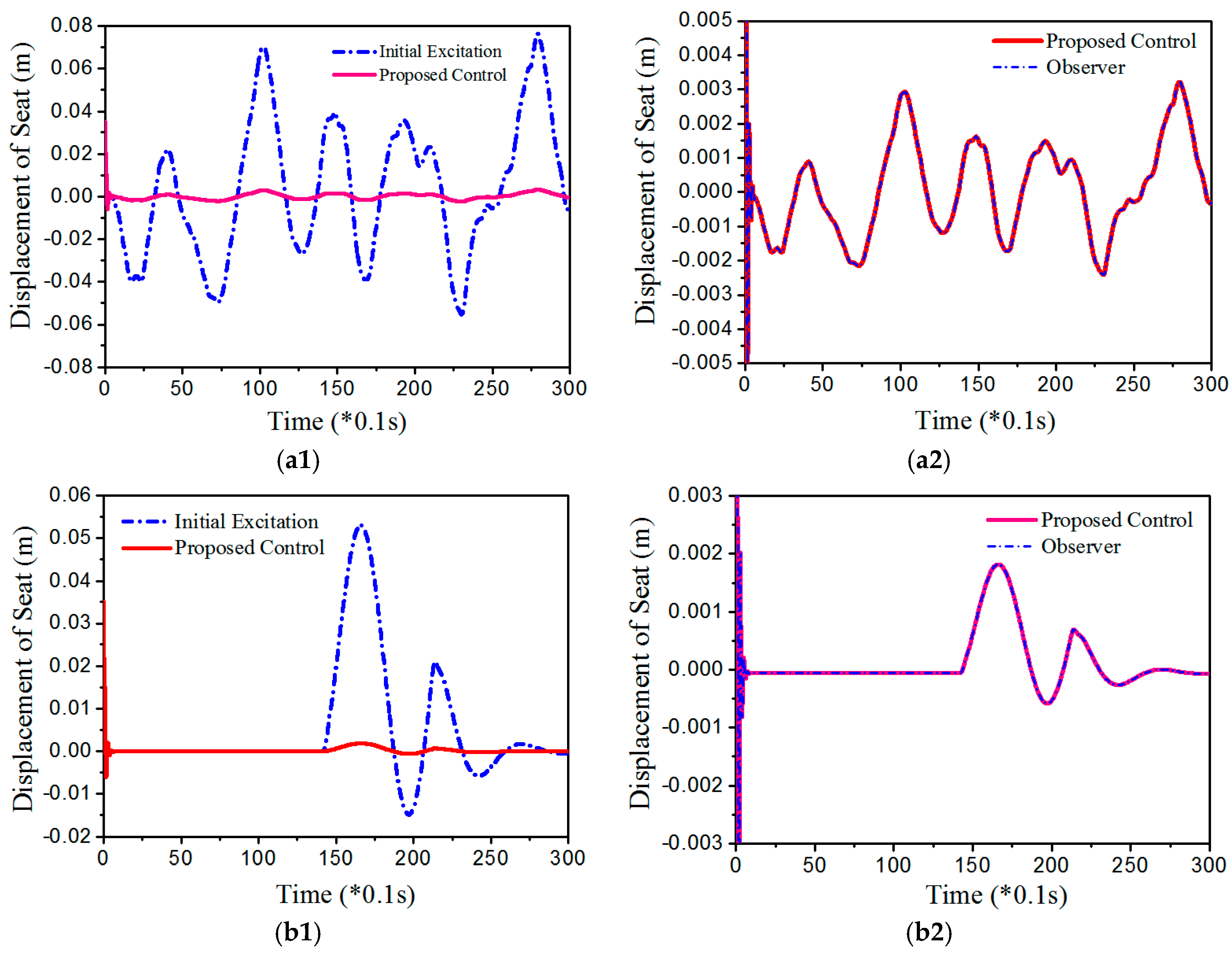
In order to investigate inherent characteristics of the proposed hybrid controller, three different excitation signals are applied to MR seat suspension system as shown in Figure 3. From the values of these signals, the proposed control scheme calculates and finds the optimal values. The displacements of the seat are presented in Figure 4. It is clearly observed that the displacements after applying the proposed controller are always less than the initial values. It is clearly also seen that that the proposed controller agrees well to the response of the observer which directly indicates assured stability of the proposed control system. From Figure 4(a1,a2), the maximal value of the displacements before controlling is approximately 0.08 m, and then after controlling, this value is less than 0.003 m. It is also identified from Figure 4(b1,b2), the maximal values of the displacement before and after controlling are 0.06 and 0.002 m, respectively. Similarly, from the results shown in Figure 4(c1,c2), the maximal values are identified by 0.06 and 0.005 m before and after controlling, respectively. From these results, it is understood that the vibrations caused from random road profiles are substantially reduced. This is one of excellent benefits of the proposed hybrid controller designed to take account of system uncertainties and external disturbances. It is remarked here that the initial constants are required for any simulation of control system. These constants are chosen by the designer. There are two ways for applying these constants. The first way is to use the initial constant as the dominant vibration, and then evaluate the control responses. The second way is to use both the initial constants and the vibration together. This approach can clearly show full view of responses of the control system. Hence, the controller can be evaluated exactly compared with the first way. Therefore, the second way is chosen in this work. On the other hand, the vibrations at the position of the driver are evaluated and presented in Figure 5. The vibration control performances at the driver position are similar to the results shown in Figure 4. This point is clearly expressed in Equation (40). It is noted here that the sliding surfaces subjected to two different road profiles go to zero during control action. This is possible since when the sliding mode converges zero, the control u given in Equation (17) is not zero because of the control u₁ given in Equation (14). The control u₁ belongs to the fuzzy neural networks model which determines the fuzzified values for the control force. This energy from the control u and the semi-active control of MR damper acts on the system. Thus, the control input always exists although the sliding surface converges to zero.

Remark 4. 

As mentioned above, the practical values shown in Figure 3 are used in experiment. However, they must be calibrated to fix the system for preventing a breakdown or dangerous accident. Hence, the results of experiment are different a little from the simulation results. This does not alter the objective of the proposed control system. It is noted that the data sample time for simulation is 30 s. In the experiment, the sample time is chosen to meet the operation of the seat′s suspension system (capacity of the hydraulic system). In this experiment, the sample time is 3 s for regular bump excitation, and 5 s for random step wave excitation. Because of the difference, it is hard to plot both the simulation and the experiment results in one figure. However, the effectiveness of the proposed controller is similar in both the simulation and experiment.

Remark 5. 

In this study, three road profiles are used in order to simulate the input signals. The road profiles shown in Figure 5a,c are collected from the real roads. The road profile shown in Figure 5b is generated from the Equation (40) given in [32]. These road profiles are used to investigate the vibrations transferred from wheels of the vehicles installed with MR dampers. Hence, these profiles can be adopted for experimental testing to emulate the practical road conditions as shown in Figure 6. It is noted that the design of vehicle suspension systems has been improved over the past decades, but this does not contribute vibration control of the seat position. Therefore, an effective seat suspension system is required to suppress the acceleration/displacement at the base of the seats. In this work, a semi-active seat suspension featuring MR damper is proposed and controlled to reduce unwanted vibrations at the seat and driver’s position.

4. Experimental Results and Discussions

An experimental apparatus for the evaluation of the proposed hybrid controller is established as shown in Figure 6. It is remarked that the equipment used for this experiment is similarly to the devices used in [17]. The signal from the sensors such as linear variable differential transformer (LVDT) transducer, accelerometers at the seat and driver are used as feedback signals to the controller. For the information about sensor characteristics, the production makers and the specific model of each sensor are given as follows: (i) a linear variable differential transformer sensor (Honeywell, type JEC-AG-DC-DC, Honeywell Inc., Morris Plains, NJ, USA) is used to measure the displacement of seat, (ii) an accelerometer (CLX Xbow MEMSIC-IMU440, MEMSIC Inc., San Jose, CA, USA) is used for measurement of the acceleration of the mass (i.e., human) on the seat, (iii) an accelerometer (Crossbow, type CXL04M1Z, Sumitomo Precision Products Co., Ltd., Amagasaki Hyogo, Japan) is used for measurement of the acceleration at the seat. The controller designed in [5] is used in this experimental evaluation as a comparative controller. This comparative controller is a kind of complicated hybrid controller whose adaptation laws are designed from the governing equation and sliding surface. In addition, the robustness function in [5] is built from the sliding mode motion and the Riccati-like equation. In this experiment, two exciting signals of the random step wave and the random regular bump are imposed via the hydraulic shaker system. Figure 7 and Figure 8 present control results obtained from the realization of the controllers using the microprocessor which consists of signal converters and controller chips. Vibration control results under the regular bump excitation are shown in Figure 7. Based on the values of the measured results, the maximum values of dynamic parameters such as displacement, velocity and acceleration can be found. The maximum displacement at the seat shown in Figure 7(a1,a2) is identified by 0.02118 and 0.03503 m for the proposed control and the control of [5], respectively. The maximum velocity at the seat is found from Figure 7(b1,b2) and the values are 0.25930 and 0.61020 m/s for the proposed control and the control of [5], respectively. The maximum acceleration at the seat is identified from Figure 7(c1,c2) and the values are 1.80093 and 2.31462 m/s² for the proposed control and the control of [5], respectively. The maximum acceleration at the driver position is evaluated from Figure 7(d1,d2) and the values are 1.03392 and 2.05639 m/s² for the proposed control and the control of [5], respectively. It is noted that the maximal values of the sinusoidal bump obtained from the proposed controller are smaller than those achieved form the controller in [5]. This is attributed to the fact that, in the proposed controller, the fuzzy neural network model is applied in which the centroid vectors are properly determined as given in Table 4. Figure 8 presents vibration control performance of MR seat suspension system subjected to the random-step-wave excitation. Similar to the previous case, the maximum values of the displacement, velocity, and acceleration of dynamic parameters at the seat and driver position can be identified from the results. The maximum displacement at the seat is found from Figure 8(a1,a2) and the values are 0.02009 and 0.04944 m for the proposed control and the control of [5], respectively. The maximum velocity at the seat is identified from Figure 8(b1,b2) and the values are 0.29681 and 0.71328 m/s for the proposed control and the control of [5], respectively. The maximum acceleration at the seat is evaluated from Figure 8(c1,c2) and the values are 2.16084 and 3.16171 m/s² for the proposed control and the control of [5], respectively. The maximum acceleration at the driver position is found from Figure 8(d1,d2) and the values are 1.67057 and 2.22271 m/s² for the proposed control and the control of [5], respectively.

From these results obtained via experimental implementation, it is clear that the proposed controller provides the better vibration control performances than the comparative controller under two different road profiles. The comparative control results are also good performances, but the performance degree is less than the proposed controller. This indicates that the proposed controller has a higher robustness under uncertain operating conditions of the control system. The proposed controller proves that the combination of two or more control logics can bring better control responses since the inherent advantages of each controller are retained to guarantee robust stability against any disturbance and the uncertainty of the system. It is noted here that according to the standard ISO 2631-1, the acceleration at the driver position should be less than 2.5 m/s² [17]. From the results presented in Figure 7 and Figure 8, the accelerations of the proposed controller shown in Figure 7(d1,d2) and Figure 8(d1,d2), are always less than the standard value of ISO 2631-1. The applied current for regular bump excitation and random-step-wave excitation is shown in Figure 9. The maximum applied currents of regular bump excitation are 1.487 A and 1.494 A for the proposed control and the control in [5], respectively. The maximum applied currents of random-step-wave excitation are 1.4908 and 1.492 A for the proposed control and the control in [5], respectively.

In order to evaluate vibration control performance, two standard factors are used in this study: ToD (Transmissibility of Displacement) and ToA (Transmissibility of Acceleration) values. The ToD values mean the ratio of the input weighted displacement to the seat frame’s weighted displacement. The floor and seat frame displacement signals are analyzed to find the vibration transmissibility response of the seat suspension. Similarly, the ToA value means the ratio of the input weighted acceleration to the seat frame’s weighted acceleration. The floor and seat frame acceleration signals are analyzed to find the vibration transmissibility response of the seat suspension. The ToD and ToA values are expressed as

$$ToD=\frac{d_{seat}}{d_{floor}}$$

(43)

$$ToA=\frac{a_{seat}}{a_{floor}}$$

(44)

where, $d_{seat}=\sqrt{\frac{1}{N}{\displaystyle \sum _{i=1}^N{d}^2{}_{seat,i}}}$, $d_{floor}=\sqrt{\frac{1}{N}{\displaystyle \sum _{i=1}^N{d}^2{}_{floor,i}}}$, $a_{seat}=\sqrt{\frac{1}{N}{\displaystyle \sum _{i=1}^N{a}^2{}_{seat,i}}}$, $a_{floor}=\sqrt{\frac{1}{N}{\displaystyle \sum _{i=1}^N{a}^2{}_{floor,i}}}$.

It is noted that the ToD and ToA values are calculated based on the root mean square equation as given in $d_{seat}$, $d_{floor}$, $a_{seat}$ and $a_{floor}$. It has been identified that the ToD values of the regular bump excitation are 0.262262, 0.289031, and 0.274320 for the proposed control, the comparative control in [5], and the control in [17], respectively. Similarly, the ToD values of the random step wave excitation are 0.349026, 0.586984 and 0.398267 for the proposed control, the comparative control in [5], and the control in [17], respectively. Similarly, from the acceleration responses, the ToA values of random step wave excitation are 0.585122, 0.732741, 0.608735 for the proposed control, the comparative control in [5], and the control in [17], respectively. The ToA values of the regular bump excitation are 0.579926, 0.699909 and 0.58324 for the proposed control, the comparative control in [5], and the control in [17], respectively. These results are summarized in

Table 5. Evaluation values of ToD and ToA.

Index	Bump Regular Excitation
	Proposed Control	Control [5]	Control [17]
ToD	0.262262	0.289031	0.274320
ToA	0.579926	0.699909	0.583241
Index	Random Step Wave Excitation
	Proposed control	Control [5]	Control [17]
ToD	0.349026	0.586984	0.398267
ToA	0.585122	0.732741	0.608735

. It is therefore concluded that the proposed hybrid adaptive controller implemented to MR seat suspension system can enhance ride comfort of the driver of commercial vehicles such as bus and truck table.

5. Conclusions

In this work, a new adaptive hybrid controller based on the H-infinity control technique, sliding mode controller and PID controller was formulated and applied to vibration control of an MR seat suspension system to demonstrate its effectiveness. In the formulation of the hybrid controller, the online interval type 2 fuzzy and the Riccati-like equation were also used for combining three controllers. The parameters of the Riccati-like equation were determined to follow the change of system based on the fuzzy model and sliding surface of the sliding mode controller. The stability of the proposed hybrid adaptive controller was then solidly proven by adopting Lyapunov stability criterion. Subsequently, the proposed controller was applied to vibration control of MR seat suspension system of commercial vehicles such as bus and truck. Control performances were evaluated through both computer simulations and experimental realization by integrating the microprocessor. In order to validate robust stability of the proposed control system, three different road profiles were adopted and used for the excitations; random bump excitation, regular bump excitation, and random-step-wave excitation. After showing the effectiveness and characteristics of the proposed controller using computer simulations, experimental tests were undertaken to achieve control results for the excited vibrations. It has been shown from experimental realization that the proposed controller can reduce unwanted vibrations at the seat and the driver position satisfying the regulation of the ISO 2631-1. The results presented in this work are quite self-explanatory, justifying that an appropriate hybrid controller which consists of several classical/modern controllers and intelligent controllers can significantly improve the effectiveness of control performances much better than the implementation of a single controller. Notably, the control effectiveness of the hybrid controller is highlighted for complicated systems subjected to parameter variations and external disturbances.

References

- Pan, Y.; Zhou, Y.; Sun, T.; Joo, M. Composite adaptive fuzzy H∞ tracking control of uncertain nonlinear systems. Neurocomputing 2013, 99, 15–24. [Google Scholar] [CrossRef]
- Li, N.; Feng, J. The design of reliable adaptive controllers for time-varying delayed systems based on improved H∞ performance indexes. J. Frankl. Inst. 2015, 352, 930–951. [Google Scholar] [CrossRef]
- Li, X.J.; Yang, G.H. Adaptive H∞ control in finite frequency domain for uncertain linear systems. J. Inf. Sci. 2015, 314, 14–27. [Google Scholar] [CrossRef]
- Lin, T.C.; Wang, C.H.; Liu, H.L. Observer-based indirect adaptive fuzzy-neural tracking control for nonlinear SISO systems using VSS and H∞ approaches. Fuzzy Sets Syst. 2004, 143, 211–232. [Google Scholar] [CrossRef]
- Yu, W.S.; Weng, C.C. H∞ tracking adaptive fuzzy integral sliding mode control for parallel manipulators. Fuzzy Sets Syst. 2015, 248, 1–38. [Google Scholar] [CrossRef]
- Wu, T.S.; Karkoub, M. H∞ fuzzy adaptive tracking control design for nonlinear systems with output delays. Fuzzy Sets Syst. 2014, 254, 1–25. [Google Scholar] [CrossRef]
- Lin, T.C.; Roopaei, M. Based on interval type-2 adaptive fuzzy H∞ tracking controller for SISO time-delay nonlinear systems. Commun. Nonlinear Sci. Numer. Simul. 2010, 15, 4065–4075. [Google Scholar] [CrossRef]
- Phu, D.X.; Shin, D.K.; Choi, S.B. Design of a new adaptive fuzzy controller and its aplication to vibration control of a vehicle seat installed with an MR damper. Smart Mater. Struct. 2015, 24, 085012. [Google Scholar] [CrossRef]
- Phu, D.X.; Shah, K.; Choi, S.B. Design of a new adaptive fuzzy controller and its implementation for the damping force control of a magnetorheological damper. Smart Mater. Struct. 2014, 23, 065012. [Google Scholar] [CrossRef]
- Phu, D.X.; Choi, S.B. Vibration control of a ship engine system using high-load magnetorheological mounts associated with a new indirect fuzzy sliding mode controller. Smart Mater. Struct. 2015, 24, 025009. [Google Scholar] [CrossRef]
- Wang, W.Y.; Chan, M.L.; Lee, T.T.; Liu, C.H. Adaptive fuzzy control for strict-feedback canonical nonlinear systems with H∞ tracking performance. IEEE Trans. Syst. Man Cybern. Part B Cybern. 2000, 30, 878–885. [Google Scholar]
- Chang, Y.C. Adaptive fuzzy-based tracking control for nonlinear siso systems via VSS and H∞ approaches. IEEE Trans. Fuzzy Syst. 2001, 9, 278–292. [Google Scholar] [CrossRef]
- Do, X.P.; Shah, K.; Choi, S.B. Damping force tracking control of MR damper system using a new direct adaptive fuzzy controller. Shock Vib. 2015, 947937, 1–17. [Google Scholar] [CrossRef]
- Yang, Y.; Zhou, C. Adaptive fuzzy H∞ stabilization for strict-feedback canonical nonlinear systems via backstepping and small-gain approach. IEEE Trans. Fuzzy Syst. 2005, 13, 104–114. [Google Scholar] [CrossRef]
- Do, X.P.; Quoc, N.V.; Park, J.H.; Choi, S.B. Design of a novel adaptive fuzzy sliding mode controller and application for vibration control of magnetorheological mount. J. Mech. Eng. Sci. 2014, 228, 2285–2302. [Google Scholar]
- Fei, J.; Juan, W.; Xin, M. Adaptive fuzzy H∞ control strategy for a micro-electromechanical system gyroscope based on the linear matrix inequality approach. J. Sys. Control Eng. 2012, 226, 1039–1049. [Google Scholar] [CrossRef]
- Do, X.P.; Choi, S.B.; Lee, Y.S.; Han, M.S. Vibration control of a vehicle’s seat suspension featuring a magnetorheological damper based on a new adaptive fuzzy sliding-mode controller. Proc. Inst. Mech. Eng. D J. Automob. Eng. [CrossRef]
- Do, X.P.; Choi, S.M.; Choi, S.B. A new adaptive hybrid controller for vibration control of a vehicle seat suspension featuring MR damper. J. Vib. Cont. 2016, 1–22. [Google Scholar] [CrossRef]
- Nguyen, S.D.; Nguyen, H.Q.; Choi, S.-B. Hybrid clustering based fuzzy structure for vibration control—Part1: A novel algorithm for building neuro-fuzzy system. Mech. Syst. Signal Process. 2015, 50, 510–525. [Google Scholar] [CrossRef]
- Nguyen, S.D.; Nguyen, H.Q.; Choi, S.-B. A hybrid clustering based fuzzy structure for vibration control-Part 2: An application to semi-active vehicle seat-suspension system. Mech. Syst. Signal Process. 2015, 56, 288–301. [Google Scholar] [CrossRef]
- Wang, X.; Liu, X.; Zhang, L. A rapid fuzzy rule clustering method based on granular computing. Appl. Soft Comput. 2014, 24, 534–542. [Google Scholar] [CrossRef]
- Karnik, N.N.; Mendel, J.M. Centroid of a type 2 fuzzy set. J. Inf. Sci. 2001, 132, 195–220. [Google Scholar] [CrossRef]
- Fayek, H.M.; Elamvazuthi, I.; Perumal, N.; Venkatesh, B. A controller based on Optimal Type-2 Fuzzy Logic: Systematic design, optimization and real-time implementation. ISA Trans. 2014, 53, 1583–1591. [Google Scholar] [CrossRef] [PubMed]
- Mendel, J.M. Computing derivatives in interval type-2 fuzzy logic systems. IEEE Trans. Fuzzy Syst. 2004, 12, 84–98. [Google Scholar] [CrossRef]
- Juang, C.F.; Tsao, Y.W. A Self-evolving interval type-2 fuzzy neural network with online structure and parameter learning. IEEE Trans. Fuzzy Syst. 2008, 16, 1411–1424. [Google Scholar] [CrossRef]
- Wu, D. Approaches for reducing the computational cost of interval type-2 fuzzy logic systems: Overview and comparisons. IEEE Trans. Fuzzy Syst. 2013, 21, 80–99. [Google Scholar] [CrossRef]
- Juang, C.F.; Chen, C.Y. Data-driven interval type-2 neural fuzzy system with high learning accuracy and improved model interpretability. IEEE Trans. Cybern. 2013, 43, 1781–1795. [Google Scholar] [CrossRef] [PubMed]
- Mendel, J.M.; Liu, X. Simplified interval type-2 fuzzy logic systems. IEEE Trans. Fuzzy Syst. 2014, 21, 1056–1069. [Google Scholar] [CrossRef]
- Liang, Q.; Mendel, J.M. Interval type-2 fuzzy logic systems: theory and design. IEEE Trans. Fuzzy Syst. 2000, 8, 535–550. [Google Scholar] [CrossRef]
- Wu, H.; Mendel, J.M. Uncertainty bounds and their use in the design of interval type-2 fuzzy logic systems. IEEE Trans. Fuzzy Syst. 2002, 10, 622–639. [Google Scholar]
- Ciccarella, G.; Dalla Mora, M.; Germani, A. A Luenberger-like observer for nonlinear systems. Int. J. Control 1993, 57, 537–556. [Google Scholar] [CrossRef]
- El Majdoub, K.; Ghani, D.; Giri, F.; Chaoui, F.Z. Adaptive semi-active suspension of quarter-vehicle with magnetorheological damper. J. Dyn. Syst. Meas. Control 2015, 137, 021010-1–021010-12. [Google Scholar] [CrossRef]
- Slotine, J.J.; Li, W. Applied Nonlinear Control; Prentice Hall: Englewood Cliffs, NJ, USA, 1991. [Google Scholar]
Figure 1.
A closed-loop of the proposed hybrid controller.
Figure 2.
Seat suspension with MR damper for a commercial bus: (a) practical model (photograph); (b) mechanical model.
Figure 3.
Excitation signals: (a) random-bump road; (b) regular-bump road; (c) random step wave road.
Figure 4.
Simulation results of the displacement xs of the seat: (a1,a2) random-bump road; (b1,b2) regular-bump road; (c1,c2) random step wave road.
Figure 5.
Simulation results of the displacement x1 of the driver: (a1,a2) random-bump road; (b1,b2) regular-bump road; (c1,c2) random step wave road.
Figure 6.
Experiment setup for vibration control of MR seat suspension system.
Figure 7.
Experiment results under regular bump excitation: (a1) displacement; (a2) enlarged view of the displacement; (b1) velocity; (b2) enlarged view of the velocity; (c1) acceleration at the seat; (c2) enlarged view of acceleration at the seat; (d1) acceleration of the driver; (d2) enlarged view of the acceleration of the driver.
Figure 8.
Experiment results under random-step-wave excitation: (a1) displacement; (a2) enlarged view of the displacement; (b1) velocity; (b2) enlarged view of the velocity; (c1) acceleration at the seat; (c2) enlarged view of the acceleration at the seat; (d1) acceleration of the driver; (d2) enlarged view of the acceleration of the driver.
Figure 9.
Applied control current: (a1,a2) regular bump excitation; (b1,b2) random-step-wave excitation.