Numerical Study on Guided Wave Propagation in Wood Utility Poles: Finite Element Modelling and Parametric Sensitivity Analysis


School of Civil and Environmental Engineering, University of Technology Sydney, Sydney NSW 2007, Australia
*
Author to whom correspondence should be addressed.
Appl. Sci. 2017, 7(10), 1063; https://doi.org/10.3390/app7101063
Submission received: 8 July 2017
/
Revised: 10 September 2017
/
Accepted: 7 October 2017
/
Published: 14 October 2017
Abstract
:Recently, guided wave (GW)-based non-destructive evaluation (NDE) techniques have been developed and considered as a potential candidate for integrity assessment of wood structures, such as wood utility poles. However, due to the lack of understanding on wave propagation in such structures, especially under the effect of surroundings such as soil, current GW-based NDE methods fail to properly account for the propagation of GWs and to contribute reliable and correct results. To solve this critical issue, this work investigates the behaviour of wave propagation in the wood utility pole with the consideration of the influence of soil. The commercial finite element (FE) analysis software ANSYS is used to simulate GW propagation in a wood utility pole. In order to verify the numerical findings, the laboratory testing is also conducted in parallel with the numerical results to experimentally verify the effectiveness of developed FE models. Finally, sensitivity analysis is also carried out based on FE models of wood pole under different material properties, boundary conditions and excitation types.
1. Introduction
Wood utility poles are widely applied to facilitate electricity transmission and distribution all over the world due to easy availability, low cost and environmental protection [1,2]. According to [3], around 5.3 million utility poles made of wood are utilised in Australia, with an appropriate value of more than $12 billion. However, because of exposure to severe environmental conditions, together with fungus and termite attack, wood poles may suffer from the internal deterioration, leading to the strength loss which may cause low reliability of power supply to support daily life.
In the last few decades, a large number of non-destructive evaluation (NDE) techniques have been developed to assess the integrity of wood structures, such as wood piles and poles [4,5,6,7,8,9,10]. Sounding is the simplest method for in-situ pole condition assessment, which employs an impact hammer to hit the pole and indicates the void based on a hollow sound. However, this method has the main disadvantage of low accuracy and reliability in results, which are subjective and mainly dependent on the experience of the operator. Furthermore, guided wave is another commonly used NDE method to evaluate the internal damage of wood poles. The guided wave can be produced by a hammer excitation and measured by the accelerometers installed at the side of the structure. Through the study on reflective wave signals, the forecast of health condition of structure will be attempted.
However, when the guided wave method is used to evaluate wood poles, the following critical problems should be considered and solved in advance. First of all, wood is a complicated natural material with anisotropic and non-homogeneous features so its material properties are highly influenced by the external environments such as moisture and temperature. As a consequence, the testing accuracy heavily relies on the understanding of wood material features and properties affecting the wave propagation behaviour. Additionally, the surrounding media is changeable during the wave propagation in the wood poles. Generally, an in-situ utility pole is 12 m long with 1.2–1.5 m embedded length underground, which means that the transmission media of wave in the pole changes from air to soil. In this case, the wave behaviour influenced by the transmission media should be considered. The last, but not the least problem, is the excitation position. Ideally, the optimal impact location is the middle top of the pole, where the excitation is able to produce pure longitudinal waves, and longitudinal wave is pretty easy to be analysed, as compared with other possible waves generated in wood poles. Nevertheless, in practical application, the top impact is not available, so the side impact at a reachable height is employed to excite the structure, where longitudinal, bending and surface waves are generated in the meantime, as well as two transmission directions of upward and downward travelling. The prerequisite of condition assessment of wood poles is to understand the complicated wave propagation in pole structure, which is also the objective of this work.
In this paper, the numerical studies are conducted to investigate the wave behaviour in in-service wood poles using finite element (FE) analysis. First of all, the FE models of wood pole with isotropic and orthotropic materials are developed considering the soil influence, respectively. Then, to verify the numerical results, experimental testing is carried out based on a 5 m long pole specimen made of wood. An impact hammer and several accelerometers are employed to excite the wave signal and capture the wave propagation response, respectively. The comparison between numerical and experimental results validates that the FE model is able to satisfactorily portray the wave patterns obtained from the experimental testing even though several signal peaks are missed. Finally, to better understand the wave behaviour in the wood pole, the parametric sensitivity analysis is undertaken to investigate the influence of material properties and excitation location on the wave propagation velocity.
2. Up-to-Date Numerical Modelling of Wooden Utility Poles
As mentioned at the outset, wood has complex mechanical behaviour with highly nonlinear performance [11]. However, in existing studies, wood is sometimes simulated as a homogeneous and isotropic material. This assumption will not be able to illustrate the practical mechanics performance [12]. For analysing the failure and fatigue behaviour of wood structures like piles or poles, it is well recognised that it is necessary to model wood as an orthotropic material with elastic-plastic behaviour based on Hill’s criterion [13,14]. Besides, Piao developed FE models to forecast the performance of the uniform-diameter wood poles subjected to the loads [15]. Five orthotropic models were developed using ANSYS and were verified with experimental results. In the research, three-dimensional (3D) 10-node tetrahedral solid element was used in the modelling of wood laminated poles, which has a nonlinear displacement behaviour, plasticity, large deflection, and large strain capabilities. The predicted deflection by these models agreed well with those of the experiments, and the predicted normal stress agreed with those calculated. Pellicane and Franco employed 3D FE models to investigate the stress distribution and failure of wood poles subjected to cantilever bending [16]. Orthotropic and isotropic material models with linear-elastic material properties were built and verified with the theoretical results. It can be concluded that orthotropic models are more sensitive to support conditions affecting the bending stress distribution near the boundary. Bulleit and Falk developed an isotropic material model to investigate the usage of guided wave velocity measurements to distinguish between strength-reducing decay and non-strength-reducing growth ring separations (ringshake). The results from the field testing and FE analysis indicated that the guided wave velocity measurements alone were not sufficient to confidently differentiate between ringshake and decay [17].
On the other hand, the soil is also a complex material, which consists of particles with various mineralogy, size and shape [18]. Therefore, soil modelling plays an essential role in pile or pole testing research, because the piles and poles are generally embedded in the soil, the boundary condition of which will directly affect the wave propagation behaviour in structures when stress wave-based NDE techniques are adopted for tests. High strain testing of piles or poles is typically performed to evaluate the driving system for assessing the static or bearing capacity. For this kind of testing, soil behaviour is always considered as elasto-plastic and simulated by the Mohr-Coulomb model to describe the stability of foundation structures. Abdel-Rahman and Achmus created numerical models to illustrate the behaviour of medium dense sand when the piles are under an inclined load [19]. Choi et al. used a Mohr-Coulomb elasto-plastic model to describe the soil behaviour and pile foundation stability when a strong earthquake occurred [20]. Moreover, low strain methods have also been developed for the integrity assessment of embedded length estimation of piles. For a very low strain level (less than 10−5), the elastic and linear behaviour of soil is obvious [21]. Accordingly, soil could be simulated as linear-elastic, which provides the most basic soil behaviour without considering the nonlinear and plastic behaviour at failure of the soil. Chow et al. adopted a linear-elastic model to describe the soil behaviour under integrity testing [22]. In this work, low strain testing is conducted and the strain level is less than 10−5. Consequently, the material constitutive in this paper will be simulated as linear-elastic. Furthermore, to effectively analyse the wave propagation in wood poles, the effect of soil-pole interaction should be also considered. For the current research on soil-pile/pole interaction, interfaces are commonly simulated in two ways, perfectly bonded interface or frictional interface. The frictional interface allows slipping and gapping between the soil and the structure, more accurately representing the practical behaviour. In this case, the Coulomb’s friction model is employed to simulate slipping and gapping in FE analysis, but it will take more calculation time and computer resources. Accordingly, if slipping and gapping is negligible or will not affect the analysis result, perfect bonding using the coupling method can be applied [23]. In the field of pile/pole testing, the soil is also considered as the linear-elastic material, the plastic deformation of which can be depicted by a series of linear springs. In this case, the slip effect between structure and soil can be neglected [24]. In ANSYS, interaction behaviour modelling can be achieved via contact analysis considering different contact conditions. Ji and Wang adopted surface contact element in ANSYS to simulate the integrity testing of a wharf pile based on one-dimensional guided wave theory [25]. The results from numerical results matched with experimental results quite well and the defects of the wharf piles could be detected accurately. The dynamic response of wharf piles caused by pulse loading can be accurately simulated by ANSYS. Interface elements (contact pairs) in ABAQUS were chosen by Miao et al. to investigate the response of a single pole when subjected to lateral soil movements [26]. These elements were allowed to separate if there was tension across the interface and the shear and normal force are set to zero once a gap is formed. Ninić et al. studied the pole-soil interaction along the pole skin under an axial loading using a 3D frictional point-to-point contact formulation, where each pole integration point was associated with an adjacent target point in the soil element [27]. It has been shown that pole responses are comparable with the analytical models he developed.
3. Modelling of Wave Propagation in Wooden Poles
To simulate the wood pole embedded in the soil and demonstrate the wave propagation behaviour in the embedded poles, three issues should be considered in numerical modelling: wood material, soil and soil-pole interaction. Adopting the proper modelling approach, the wave behaviour in the embedded timber pole will be investigated.
3.1. Modelling of Wood Material
Wave propagation in wood is a complicated dynamic procedure controlled by the properties, orientation and microstructure of the fiber, and perhaps more importantly, by the geometry of the material [28]. As a result, accurate modelling of wood materials is the priority issue to get insight into wave propagation behaviour in wood poles.
To investigate the influence of the material characteristics on the wave behaviour, FE modelling of material characteristics should be divided into three categories: isotropic, transversely isotropic and orthotropic. Isotropic material has the uniform values of a property in all directions, none of the properties depend on the orientation and the material is perfectly rotationally symmetrical. Transversely isotropic material has the uniform properties in one plane and different properties in the direction normal to this plane. An orthotropic material has at least two symmetric orthogonal planes, where material property is unique and independent in the direction within each plane. A material without any symmetric planes in defined as orthotropic material [29,30].
According to the general Hooke’s law, the orthotropic material is able to be mathematically expressed using the following matrix:
where ε denotes the elastic strain vector; γ denotes the shear strain vector; σ denotes the stress vector; E denotes elastomer modulus; G denotes the shear modulus; v denotes the Poisson’s ratio. The subscripts L, R and T denote the grain directions, with L representing the longitudinal direction, R representing the radius direction and T representing the tangential direction, shown in Figure 1.
The matrix can be simplified to the following equation:
where {ε} and {σ} denotes the strain and stress tensors, respectively; [C]orth denotes a 6 × 6 orthotropic elastic matrix. For the orthotropic material, the following expression is valid:
Accordingly, the orthotropic elastic matrix [C]orth is able to be expressed as a symmetric matrix, with nine parameters required to be defined as the wood material properties.
3.2. Modelling of Soil
In the field, the wood utility poles are generally embedded in the soil. Under this condition, boundary influences from the surrounding soil should also be considered so as to accurately characterise the wave propagation. In this work, to study the effect of soil modelling method, two models are built up based on a 5 m long pole using two different soil modelling methods: elastic linear model (linear) and Drucker-Prager model (nonlinear). Table 2 gives the all the properties of materials and Figure 2 compares the calculated acceleration responses of two models, when the sensor is located at 1.6 m from the bottom of the pole. In this comparison, the wave velocity is considered as main evaluation index, the change of which is generally caused by internal damage of the wood pole.
In Figure 3, the dashed curve shows the results of the elastic linear soil model and the solid curve denotes the results using the Drucker-Prager model. The comparative results demonstrate that different soil modelling methods may lead to some difference in the structural responses. However, the difference is just about the wave amplitude rather than the wave pattern. It can also be found that the acceleration amplitude of the Drucker-Prager model is larger than that of the linear elastic model, even though the locations of wave peaks appear at almost the same time point. This result contributes to the conclusion that different soil modelling methods have less effect on the accuracy of wave propagation in this work and the linear elastic model is reasonable to portray the soil performance.
3.3. Modelling of Soil-Pole Interaction
Interaction behaviour simulation between soil and wood utility pole is another important issue in modelling since it will affect the results directly. In the FE analysis, the modelling of interaction behaviour can be realised via the contact analysis considering different contact conditions, in which the restraints and contact conditions should be carefully defined ahead of time.
There are two commonly used contact analysis methods reported in FE modelling. One is perfectly bonded contact analysis, which is on basis of small deflection or rotation and supposes that two components are bonded together without friction [32]. The other one is frictional contact, which indicates that the contact surfaces could be divided and regarded as nonlinear behaviour. There are two main difficulties during the analysis: (1) the contact region is not predictable due to the many factors such as loading, material properties and boundary conditions; (2) the friction should be considered and the responses may be chaotic, which will make the solution not convergent. In this study, both bonded and frictional contacts are employed to demonstrate the contact state in ANSYS. The Lagrange Multiplier method is applied on the contact normal while the penalty method is applied on the frictional plane, which allows a very small amount of slip for a sticking contact condition.
Moreover, the boundary condition of wood pole plays a significant role on the wave propagation behaviour. The hard boundary will change the phase direction of wave propagation compared with the soft boundary. To clearly illustrate this phenomenon, two numerical models with the length of 12 m and average diameter of 0.3 m are created. The model with a free end is achieved by modelling the pole hanging through two steel cables while the fixed boundary is achieved by coupling the contact node of the pole and bedrock. The hammer impact is applied on the top centre of the pole and the sensor is deployed at the top side of the pole, as shown in Figure 3. The mesh conditions are exactly same for the contact surface to make use of the coupling method, shown in Figure 4.
The friction interface representing high nonlinear behaviour allows modelling of slipping and gapping between the soil and the pole, therefore taking more calculation time and computer resources. However, if the slipping and gapping is negligible or will not affect the analysis results, perfect bonding can be considered [23,33]. In this study, negligible slipping and gapping between soil and pole is caused by low strain testing. In this case, perfect bonding is considered to simulate the interaction behaviour, which is achieved by coupling the contact node of the pole and bedrock. Figure 4 and Figure 5 show the mesh conditions of FE model for the contact surface.
A measurement sensor is located on the top of the pole and a hammer excitation is applied on the top centres of two models. The material properties for different structural components are shown in Table 3. Figure 5 compares the results of wave behaviour from two different boundary conditions. It is noticeable that the incident waves, directly generated by the hammer impact, uniformly propagate until they arrive at the boundary of the pole. For the free end boundary condition, the wave reflects back from the boundary and keeps the same phase direction as shown by the red solid curve in the figure: all the peaks are in the same direction. However, for the bedrock boundary condition, when the wave reflects back, the phase direction is opposite to the incident wave and the phase changes again when it gets to the hard boundary as illustrated by the blue dashed curve: the peak directions are opposite to each other. This phenomenon can be intuitively explained in accordance with Hirose and Lonngren’s wave theory: when the wave pulse approaches the fixed end, the internal restoring forces which allow the wave to propagate exert an upward force on the end of the pole [34]. However, the bedrock is fixed and should be exerting an equal downward force on the end of the pole. This new force generates a wave pulse that propagated back with the same velocity and amplitude as the incident wave, but with opposite polarity.
3.4. Experimental Validation
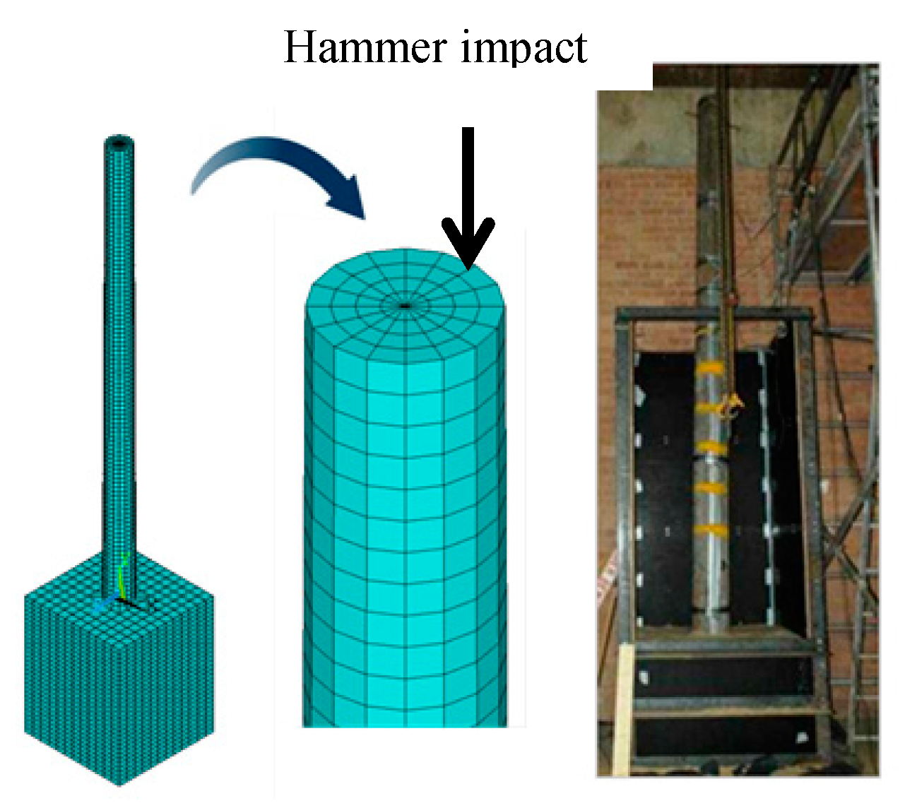
To validate the performance of the FE model to describe the wave propagation in the wood poles with surrounding soil, the laboratory testing is conducted to make the comparison with simulation results. In this study, a 5 m long pole embedded in sand by 1 m is employed due to the limitation of the ceiling height in the laboratory. The dimensions of the cage that stores the sands are 1.2 m by 1.3 m by 3 m, in which 3 m is the height of the cage. Figure 6 gives the makeup of NDE system for pole testing, which consists of a modally tuned impact hammer, multiple sensors (accelerometers), a multi-channel signal conditioner, a multi-channel data acquisition system and a computer equipped with signal acquisition software. For the guided wave testing, the adopted impact hammer (PCB Piezotronics, Depew, NY, USA) is a PCB model HP086C05 of sensitivity 0.24 mV/N. A load cell connected with hammer is used to measure the impact force to the structure. To record the structural response, piezoelectric accelerometers (PCB Piezotronics, Depew, NY, USA) with PCB model 352C34 are employed, which have the high sensitivity of 100 mV/g as well as the bandwidth from 0.2 Hz to 10 kHz. To amplify and tune the signals of the modal hammer and the piezoelectric accelerometers, a 12-channel signal conditioner (PCB Piezotronics, Depew, NY, USA) with model PCB 483B03 is utilised. The data acquisition system (National Instruments, Austin, TX, USA) employed is a middle range 8-channel system with 12-bit 4 M sample/sec per channel with model NI PCI6133. In this work, the sample frequency for NDE of wood pole is set as 1 MHz. For data processing and analysis, a personal computer (Dell Inc., Round Rock, TX, USA) equipped with NI software LabVIEW (National Instruments, Austin, TX, USA) is adopted.
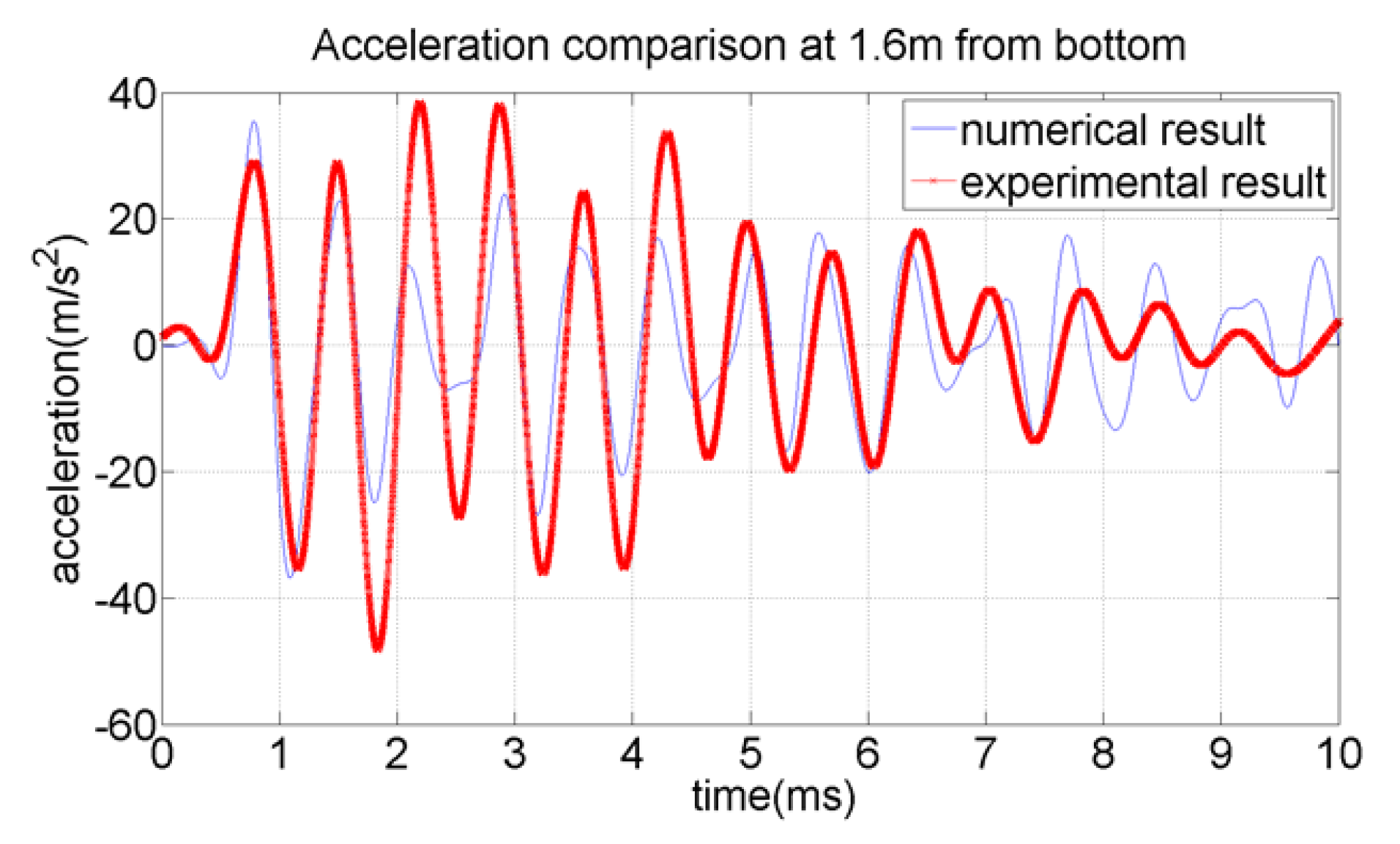
Experimental setup and the FE model designed by ANSYS (ANSYS Inc., Canonsburg, PA, USA) are given in Figure 7. In this comparative study, both frictional contact and bonded contact are considered to represent the contact states. Figure 8 and Figure 9 respectively shows response comparisons between experimental results and the results from numerical models with frictional and bonded contacts, when the signals are captured from the sensor located at 1.6 m from the bottom of the pole. The time corresponding to the peak points reveal the arrival and reflection of wave propagation and it is a significant feature to illustrate the wave behaviour. As a consequence, the time when peaks appear is the most critical issue for the comparison. In the figures, the red thick curve presents the experimental result while the blue thin curve indicates the numerical result. After comparing the results from the model of frictional contact as well as bonded contact, it is found that the wave pattern from the model of bonded contact is more consistent with the experimental result. Moreover, the curve for the model using friction contact misses several peaks compared with the experimental result. Therefore, bonded contact will be used in further study to simulate interaction behaviour between the wood pole and the soil.
To get the optimal material model representing the wood pole, further validation is conducted, in which isotropic, orthotropic and transversely isotropic material models are created and compared with experimental results. Figure 10 gives the corresponding response results obtained from the sensor located at 1.6 m from the bottom of the pole. It is noticeable that the wave responses of isotropic material model and transversely isotropic material model are quite close to each other for both wave pattern and time when the peaks appear. It also can be observed that even though the response of orthotropic material model misses some clear peaks, the times when peaks appear are more consistent with experimental results than other material model.
4. Parameter Sensitivity Analysis
Wood properties will be remarkably influenced by the age, diversity and variation between and within different species of woods in terms of the biological origin. In this study, property parameters used are obtained from the wood specimen provided by our industry partner AUSGRID (Sydney, New South Wales, Australia), the type of which is Spotted Gum. The elastic modulus is increased from 18,000 MPa for the green wood to 23,000 MPa for the dry wood; the density is declined from 1150 kg/m3 for the green wood to 950 kg/m3 for the dry wood. With the changing environmental condition, the material properties vary as well. Generally, the surface and internal damages are able to result in the variations of material properties. If the wood utility poles have been attacked by fungi and decay, the parameters of material properties such as elastic modulus and density will be changed. As a result, the wave behaviour in the decayed pole will be different from that in the healthy pole. This phenomenon may provide a fingerprint to detect the inner damage of the wood poles. Thus, investigation of material property influencing the wave propagation behaviour is another important issue. Consequently, in this work a parametric study is required to be conducted, in which elastic modulus, density and Poison’s ratio are regarded as the candidate parameters that will be changed by the environmental factors [31]. Moreover, wave velocity of the incident wave is considered as the index to evaluate the change of wave propagation behaviour. One important issue to be noted is that the velocity of the arrival wave is different from that of the reflected wave because of the tapered shape of the pole.
In this study, the wave signals are obtained from a 5 m wood pole with the excitation applied on the top centre. The wave velocity is calculated using the first arrival wave signals that are captured by a group of measurement points. To get an accurate wave velocity, 40 points are measured in the longitudinal direction between the ground level and 1.5 m above ground level. After this, the time step is set according to the minimum grid point distance and wave velocity. The simulation of the hammer impact is based on the experimental result and the cubic spline interpolation method is used to get enough impact points. Element SOLID 185 is used for general 3D modelling of solid homogeneous structures in ANSYS. Then, acceleration responses of the selected points are calculated using quadratic differential method. Figure 11 gives an instance of time-displacement relationships at eight specific measurement points. In the figure, the first peaks represent the time when the wave reach the specific point. It is clearly seen that all the peaks connected with a line and the slope of this line indicates the mean velocity that the guided wave propagates in the pole. Using this method, the wave velocity can be calculated and compared under different material parameter conditions.
4.1. Effect of Elastic Mdulus on Wave Behaviour
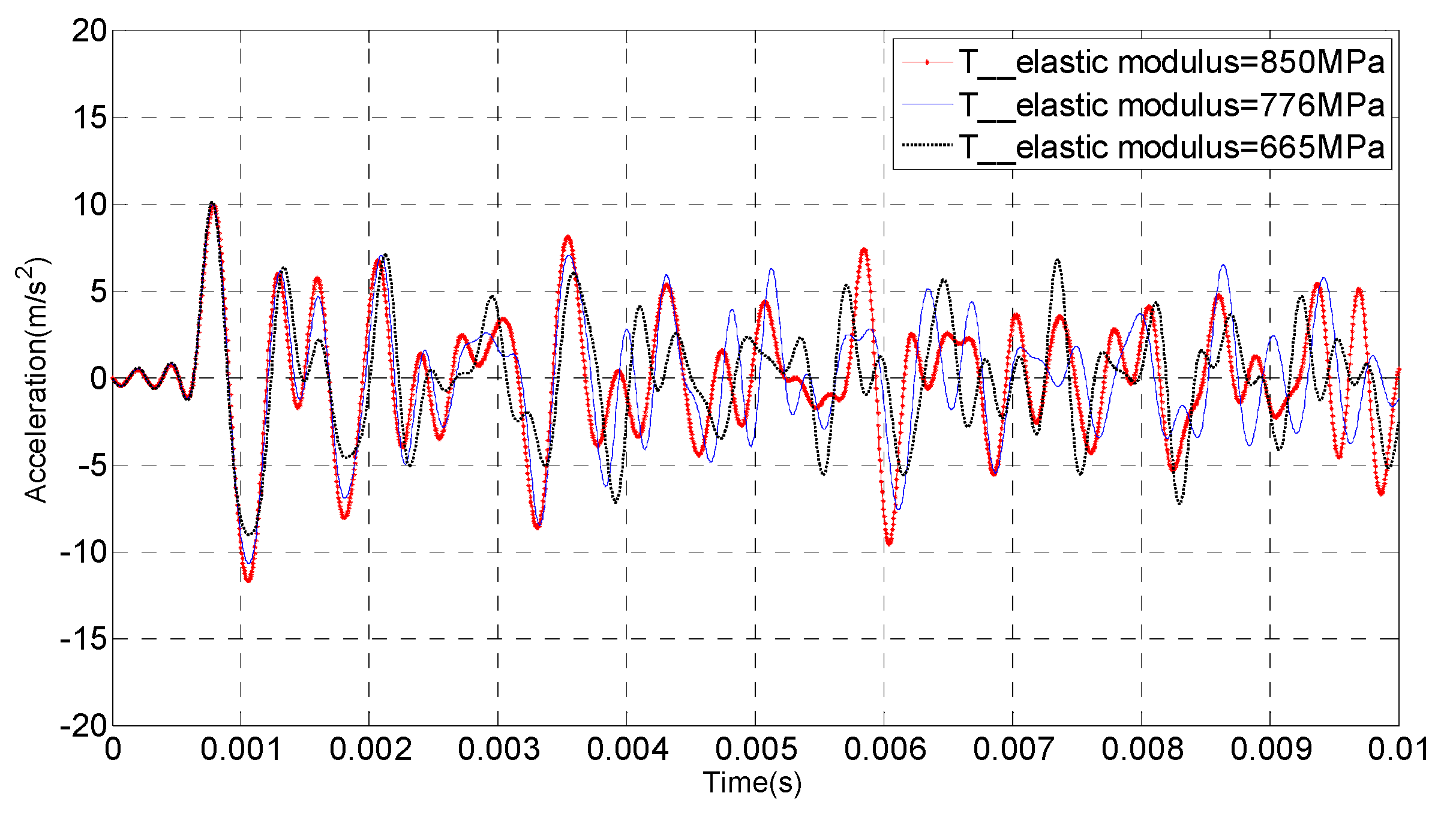
In this work, both isotropic and orthotropic models are considered to study the influence of elasticity modulus on the wave propagation in the wood pole. The parameter values are selected within the range of elastic modulus for Spotted Gum, which are shown in Table 4. As all we know, the elastic modulus for orthotropic material is free of three orthogonal axes. As a consequence, all three directions are considered to find out the effect of change in elastic modulus in each direction on the wave velocity. Figure 12 shows the acceleration responses of wood pole isotropic models corresponding to three elastic modulus values 23,000, 21,000 and 18,000 MPa. It is noticeable that when other properties such as density and Poisson’s ratio are determined, the lower elastic modulus will result in a lower wave velocity. Moreover, it is clearly noted that the delay of wave peaks appearing is more obvious within the three materials after the waves travel up and down the poles several times. The similar phenomenon can also be found in the orthotropic material model in the longitudinal direction, shown in Table 5 and Figure 13.
For the orthotropic material model, the elastic modulus in the longitudinal direction plays a significant role in changing wave velocity, and the response phenomenon is quite similar to that of the isotropic material model. However, in the radial and tangential directions, the changes of elastic modulus provide slight effect on the wave velocity. The corresponding results are shown in Figure 14 and Figure 15. It is clearly observed that the first peaks of the curves are totally overlapped, which means that the wave propagation will less influenced by the elastic modulus changes in the radial and tangential directions.
4.2. Effect of Density on Wave Behaviour
Apart from the effect of elastic modulus on wave behaviour, the parameter of density is also investigated. Similar to the elastic modulus, the densities used in this study are selected within the range of density for Spotted Gum, which are 950 kg/m3, 1050 kg/m3 and 1150 kg/m3. The isotropic and orthotropic models are imported, respectively. The same measurement point as the elastic modulus study is used to record the time history of wave propagation.
Figure 16 and Figure 17 display the behaviours of wave propagation with different densities for isotropic and orthotropic material models, respectively while Table 6 and Table 7 give the corresponding wave velocities. It is clearly seen from the figures that higher wave velocity can be obtained from the model with lower density regardless of the material characteristics. It should also be noticed that decay of wood will lead to the strength loss at first and then a gradual decrease in the rate of the strength loss at higher weight losses. In this study, the density range is within the intact pole of Spotted Gum. The lower limit of the density is still higher than intact soft wood. If there is decay in the wood, the density of the decayed wood should be much lower than the intact wood. Accordingly, a wider range of density parameter should be studied in future for damage detection.
4.3. Effect of Poisson’s Ratio on Wave Behaviour
The Poisson’s ratio is generally set as 0.3 for the isotropic material model. Because there is no reference range of Poisson’s ratio for the same species of wood, 0.35 is set for comparison in the isotropic material model. However, in the orthotropic model, three independent Poisson’s ratios obtained from related literature are firstly defined for three directions, and then the Poisson’s ratios obtained from experimental testing are used for wave to investigate the behaviour under different sets of Poisson’s ratio. The same measurement points mentioned above are used to indicate the time history. Table 8 and Table 9 give the analysis results in both isotopic and orthotropic models, and Figure 18 and Figure 19 show the corresponding wave propagation behaviours. In the isotropic material model, it can be concluded that the longitudinal wave velocity did not change too much due to the variation of Poison’s ratio. In the orthotropic model, it can be observed that the Poisson’s ratio has obvious variation in the tangential direction that leads to the corresponding change in the longitudinal wave velocity, even though the Poisson’s ratios in other two directions are quite similar. Therefore, it can be concluded that the longitudinal wave velocity is more sensitive to the Poisson’s ratio in the orthotropic material model than the isotropic material model.
4.4. Effect of Excitation Position on Wave Behaviour
One of the most challenging issues in this work is caused by the practical restriction on where guided waves can be generated. In the laboratory testing, impact on the top of a 5 m long wood pole generates the pure longitudinal wave, making the analysis of the wave behaviour straightforward. To investigate the wave behaviour caused by the top excitation, both isotropic and orthotropic numerical models are created. The cylindrical pole is modelled as a tapered shape with 1 m soil embedment. The diameter of the top is 270 mm and the bottom is 300 mm. Figure 20 portrays the wave propagation in the pole with top excitation for both isotropic and orthotropic models. It is noticeable that the wave behaviours for both models are quite similar, even though their material characteristics are definitely different.
However, most in-situ wood poles are 12 m long with 1.2–1.5 m embedment length underground, making the top excitation unfeasible because of practical limitations. Hence, in practice the excitation is usually imparted at a reachable location from the ground level with a certain of angle through a waveguide, which may result in two types of waves: longitudinal wave and bending wave as well as two directional wave propagations: upward and downward. To study this complicated wave behaviour, a full-sized wood pole model with 12 m length is built up. The pole is of tapered cylindrical shape and the top and bottom diameters are 228 mm and 300 mm, respectively. The impact excitation is generated at the location of 1.5 m above the ground with the angle of 45 degrees. Similarly, both isotropic and orthotropic models are generated, and the wave traces are shown in Figure 21. It is clearly observed that the up-going and down-going waves are generated simultaneously in the isotropic material model. Figure 22 shows a close-view of wave traces in the isotropic material model based on a fixed sensor (SN6), which is deployed at 400 mm above the soil level. It is obviously seen that the travel-down wave will be first captured by the sensor, which is recorded as first peak denoted by 1a. Then, the wave will be reflected from the bottom of the pole and captured by the same sensor as second peak denoted by 2a. At the same time, the travel-up wave reflected from the top of the wood pole will then arrive at the sensor as its first peak denoted by 1b, followed by its reflections from the bottom of the pole as its second peak denoted by 2b. Also, the figure indicates wave propagation in the soil which is below the pole. From the interface between the pole and soil (dashed line), it can be clearly observed that some of the incident waves are reflected by the bottom boundary of the pole while some of them are refracted into the soil. According to the wave trace, it can be seen that the wave travelling in the pole captured by the sensor will not be affected by the wave reflected from the boundary of the soil, because the wave velocity in the soil is extremely low and the reflected energy is also very small. Therefore, they can difficultly be detected by the sensor within the recoding time. On the other hand, the wave behaviour in the 12 m orthotropic material pole model with side excitation is pretty much complicated. It is noticeable that from the impact point, two types of waves are generated simultaneously: longitudinal and bending waves. Additionally, different modes of waves are generated because of the orthotropic characteristic of the wood, which means that reflection and refraction happen in the meantime inside the orthotropic material. Due to different types of waves with various modes, reflected wave identification becomes challenging. Accordingly, further investigation in signal processing is necessary to effectively separate longitudinal and bending waves as well as different modes.
5. Conclusions
In this work, a series of numerical studies have been conducted to investigate the wave propagation behaviour in the wood poles. Two interfacial methods, namely, friction contact and bonded contact, were proposed to simulate the interfacial behaviour between a wood pole and its surrounding soil for guided wave propagation. Experimental testing was also conducted to verify the numerical findings. The results showed that the bonded contact method can produce better overall wave propagation patterns in simulating the guided wave behaviour in the wood pole, even though the frictional contact method is able to accurately generate first two peaks of the wave pattern, which is crucial in determination of the underground embedment length. Then, parametric sensitivity is conducted to investigate the relationships between wave propagation behaviour and material properties as well as the excitation location. The results show that higher elastic modulus in the longitudinal direction always generates higher guided wave velocity regardless of the material characteristics while elastic modulus change in the radial or tangential direction has little effect on the wave propagation. Unlike the elastic modulus, the density has reverse phenomenon that lower density will yield higher wave velocity despite the material characteristics. Besides, the change of Poisson’s ratio has much more influence on wave velocity in the orthotropic material model than the isotropic material model. For the excitation location, the wave propagation in the isotropic material model is clear and can be easily analysed despite the change of excitation location due to the simplicity of the material characteristics. For the orthotropic material model, complicated wave patterns occur because of the generation of different types of waves and different modes of waves, which makes the signal analysis very complex. Furthermore, hammer impact excitation generates broad-band frequency signals, and accordingly, the generated waves in a wood pole possess a wide frequency range. To solve this issue, narrow-band signals should be considered in the following study. For the purpose of damage detection in wood utility poles, wave behaviour in damaged wood poles and advanced damage identification technique should also be investigated in the next stage. Besides, the damping of the soil and the moisture factor, that can directly influence the mechanical behaviour of the wood, will be also considered in the FE modelling, and more experimental tests will be conducted to further verify the performances of the proposed FE models.
Acknowledgments
This research is supported by University of Technology Sydney via Faculty of Engineering & Information Technology (FEIT) Blue Sky project. The authors would like to thank the financial support from the funding body.
Author Contributions
Yang Yu and Ning Yan designed the finite element models and conducted experimental testing; Ning Yan analysed the model parameter sensitivities; Yang wrote the paper.
Conflicts of Interest
The authors declare no conflict of interest.
References
- Tallavo, F.; Cascante, G.; Pandey, M.D. Experimental verification of an orthotropic finite element model for numerical simulations of ultrasonic testing of wood poles. Eur. J. Wood Wood Prod. 2017, 75, 543–551. [Google Scholar] [CrossRef]
- Yu, Y.; Li, J.; Yan, N.; Dackermann, U.; Samali, B. Load capacity prediction of in-service timber utility poles considering wind load. J. Civ. Struct. Health Monit. 2016, 6, 385–394. [Google Scholar] [CrossRef]
- Rahman, A.; Chattopadhyay, G. Soil factors behind inground decay of timber poles: Testing and interpretation of results. IEEE Trans. Power Deliv. 2007, 22, 1897–1903. [Google Scholar] [CrossRef] [Green Version]
- Nassr, A.A.; El-Dakhakhni, W.W.; Ahmed, W.H. Biodegradation and debonding detection of composite-wrapped wood structures. J. Reinf. Plast. Compos. 2010, 29, 2296–2305. [Google Scholar] [CrossRef]
- Riggio, M.; Macchioni, N.; Riminesi, C. Structural health assessment of historical timber structures combining non-destructive techniques: The roof of Giotto’s bell tower in Florence. Struct. Control Health Monit. 2017, 24, e1935. [Google Scholar] [CrossRef]
- Yu, Y.; Dackermann, U.; Li, J.; Subhani, M. Condition assessment of timber utility poles based on a hierarchical data fusion model. J. Comput. Civ. Eng. 2016, 30, 1–13. [Google Scholar] [CrossRef]
- Ryden, M.; Hanning, M.; Corcoran, A.; Lind, F. Oxygen Carrier Aided Combustion (OCAC) of wood chips in a semi-commercial circulating fluidized bed boiler using manganese ore as bed material. Appl. Sci. 2016, 6, 347. [Google Scholar] [CrossRef]
- Riggio, M.; Sandak, J.; Franke, S. Application of imaging techniques for detection of defects, damage and decay in timber structures on-site. Constr. Build. Mater. 2015, 101, 1241–1252. [Google Scholar] [CrossRef]
- Faggiano, B.; Marzo, A. A method for the determination of the timber density through the statistical assessment of ND transverse measurements aimed at in situ mechanical identification of existing timber structures. Constr. Build. Mater. 2015, 101, 1235–1240. [Google Scholar] [CrossRef]
- Lanata, F. Monitoring the long-term behaviour of timber structures. J. Civ. Struct. Health Monit. 2015, 5, 167–182. [Google Scholar] [CrossRef]
- Lu, M.L. Nonlinear behavior of wood pole structure. In Proceedings of the IEEE PES 12th International Conference on Transmission and Distribution Construction, Operation and Live-Line Maintenance, Providence, RI, USA, 16–19 May 2011. [Google Scholar]
- Subhani, M.; Li, J.; Samali, B.; Crews, K. Reducing the effect of wave dispersion in a timber pole based on transversely isotropic material modelling. Constr. Build. Mater. 2016, 102, 985–998. [Google Scholar] [CrossRef]
- Serrano, E.; Gustafsson, J.; Larsen, H.J. Modeling of finger-joint failure in glued-laminated timber beams. J. Struct. Eng. ASCE 2001, 127, 914–921. [Google Scholar] [CrossRef]
- Junior, C.C.; Molina, J.C. Numerical modeling strategy for analyzing the behaviour of shear connectors in wood–concrete composite systems. In Proceedings of the 11th World Conference on Timber Engineering, Trento, Italy, 20–24 June 2010. [Google Scholar]
- Piao, C.; Shupe, T.F.; Tang, R.C.; Hse, C.Y. Finite element analysis of wood laminated composite poles. Wood Fiber Sci. 2005, 37, 535–541. [Google Scholar]
- Pellicane, P.J.; Franco, N. Modeling wood pole failure. Wood Sci. Technol. 1994, 28, 219–228. [Google Scholar] [CrossRef]
- Bulleit, W.M.; Falk, R.H. Modeling stress wave passage times in wood utility poles. Wood Sci. Technol. 1985, 19, 183–291. [Google Scholar] [CrossRef]
- Liu, M.D.; Carter, J.P.; Airey, D.W. Sydney soil model. I: Theoretical formulation. Int. J. Geomech. 2011, 11, 225–238. [Google Scholar] [CrossRef]
- Abdel-Rahman, K.; Achmus, M. Numerical modelling of combined axial and lateral loading of vertical piles. In Proceedings of the 6th European Conference on Numerical Methods in Geotechnical Engineering, Graz, Austria, 6–8 September 2006. [Google Scholar]
- Choi, J.I.; Kim, S.H.; Kim, M.M.; Kwon, S.Y. 3D dynamic numerical modeling for soil-pile-structure interaction in centrifuge tests. In Proceedings of the 18th International Conference on Soil Mechanics and Geotechnical Engineering, Paris, France, 2–6 September 2013. [Google Scholar]
- Luna, R.; Jadi, H. Determination of dynamic soil properties using geophysical methods. In Proceedings of the First International Conference on the Application of Geophysical and NDT Methodologies to Transportation Facilities and Infrastructure, St. Louis, MO, USA, 11–15 December 2000. [Google Scholar]
- Chow, Y.K.; Phoon, K.K.; Chow, W.F.; Wong, K.Y. Low strain integrity testing of piles: Three-dimensional effects. J. Geotech. Geoenviron. 2003, 129, 1057–1062. [Google Scholar] [CrossRef]
- Balendra, S. Numerical Modelling of Dynamic Soil-Pile-Structure Interaction. Master’s Thesis, Washington State University, Pullman, WA, USA, December 2005. [Google Scholar]
- Li, G.; Motamed, R. Finite element modeling of soil-pile response subjected to liquefaction-induced lateral spreading in a large-scale shake table experiment. Soil Dyn. Earthq. Eng. 2017, 92, 573–584. [Google Scholar] [CrossRef]
- Ji, Y.; Wang, Y. Numerical simulation and method for a wharf pile integrity test based on ANSYS/LS-DYNA. J. Vib. Shock 2010, 29, 199–205. (In Chinese) [Google Scholar]
- Miao, L.; Goh, A.; Wong, K.; Teh, C. Three-dimensional finite element analyses of passive pile behaviour. Int. J. Numer. Anal. Methods Geomech. 2007, 30, 599–613. [Google Scholar] [CrossRef]
- Ninić, J.; Stascheit, J.; Meschke, G. Beam-solid contact formulation for finite element analysis of pile-soil interaction with arbitrary discretization. Int. J. Numer. Anal. Methods Geomech. 2014, 38, 1453–1476. [Google Scholar] [CrossRef]
- Xu, H.; Xu, G.; Wang, L.; Yu, L. Propagation behavior of acoustic wave in wood. J. For. Res. 2014, 25, 671–676. [Google Scholar] [CrossRef]
- Ohmichi, M.; Noda, N.; Sumi, N. Plane heat conduction problems in functionally graded orthotropic materials. J. Therm. Stress. 2017, 40, 747–764. [Google Scholar] [CrossRef]
- Luo, J.; You, C.; Zhang, S.; Chung, K.L.; Li, Q.; Hou, D.; Zhang, C. Numerical analysis and optimization on piezoelectric properties of 0–3 type piezoelectric cement-based materials with interdigitated electrodes. Appl. Sci. 2017, 7, 233. [Google Scholar] [CrossRef]
- Bootle, K.R. Wood in Australia: Types, Properties and Uses; McGraw-Hill Australia Pty Ltd.: Sydney, Australia, 1983. [Google Scholar]
- Gupta, B.K.; Basu, D. Response of laterally loaded rigid monopiles and poles in multi-layered elastic soil. Can. Geotech. J. 2016, 53, 1281–1292. [Google Scholar] [CrossRef]
- Gupta, B.K.; Basu, D. Analysis of laterally loaded rigid monopiles and poles in multilayered linearly varying soil. Comput. Geotech. 2016, 72, 114–125. [Google Scholar] [CrossRef]
- Hirose, A.; Lonngren, K.E. Introduction to Wave Phenomena; Krieger Publishing Company: Malabar, FL, USA, 2003; pp. 223–235. [Google Scholar]
Figure 1.
Three dimensional structure of wood.

Figure 2.
Comparison of numerical results according to different soil modelling methods.

Figure 3.
Finite Element (FE) model with the fixed boundary.

Figure 4.
Mesh geometry of FE model for the contact surface.

Figure 5.
Wave comparison between two different boundary conditions.

Figure 6.
Testing equipment: (a) Impact hammer; (b) Accelerometers; (c) Signal conditioner; (d) Data acquisition system; (e) Laptop with LabVIEW.
Figure 6.
Testing equipment: (a) Impact hammer; (b) Accelerometers; (c) Signal conditioner; (d) Data acquisition system; (e) Laptop with LabVIEW.

Figure 7.
Experimental setup and the FE model.

Figure 8.
Comparison between experimental and numerical results using the frictional contact method.
Figure 8.
Comparison between experimental and numerical results using the frictional contact method.

Figure 9.
Comparison between experimental and numerical results using the bonded contact method.

Figure 10.
Response comparison between results from three FE models and experimental measurements.

Figure 11.
Diagram of point vs time.

Figure 12.
Effect of elastic modulus on wave behaviour in the isotropic material model.

Figure 13.
Effect of elastic modulus in the longitudinal direction on wave behaviour in the orthotropic material model.
Figure 13.
Effect of elastic modulus in the longitudinal direction on wave behaviour in the orthotropic material model.

Figure 14.
Effect of elastic modulus in the radial direction on wave behaviour in the orthotropic model.
Figure 14.
Effect of elastic modulus in the radial direction on wave behaviour in the orthotropic model.

Figure 15.
Effect of elastic modulus in the tangential direction on wave behaviour in the orthotropic model.
Figure 15.
Effect of elastic modulus in the tangential direction on wave behaviour in the orthotropic model.

Figure 16.
Wave propagation behaviours with different densities in isotropic material model.

Figure 17.
Wave propagation behaviours with different densities in orthotropic model.

Figure 18.
Poisson’s ratio influences on wave behaviour in isotropic material model.

Figure 19.
Poisson’s ratio influences on wave behaviour in orthotropic material model.

Figure 20.
Wave trace of a 5 m pole for top excitation with (a) isotropic and (b) orthotropic material models.
Figure 20.
Wave trace of a 5 m pole for top excitation with (a) isotropic and (b) orthotropic material models.

Figure 21.
Wave trace of a 12 m pole for side excitation with (a) isotropic and (b) orthotropic material models.
Figure 21.
Wave trace of a 12 m pole for side excitation with (a) isotropic and (b) orthotropic material models.

Figure 22.
Wave trace in 12 m wood pole and soil.


Table 1.
Properties for orthotropic and transversely isotropic materials.
| Material Type | Elastic Modulus (MPa) | Shear Modulus (MPa) | Poison’s Ratio | ||||||
|---|---|---|---|---|---|---|---|---|---|
| ER | ET | EL | GLR | GRT | GLT | VRL | VRT | VTL | |
| Orthotropic | 1955 | 850 | 23,000 | 1513 | 357 | 1037 | 0.040 | 0.682 | 0.023 |
| Transversely isotropic | 1955 | 1955 | 23,000 | 1513 | 581 | 1513 | 0.023 | 0.682 | 0.023 |
Table 2.
Material properties of the soil models.
| Model | Density (kg/m3) | Elastic Modulus (MPa) | Poison’s Ratio |
|---|---|---|---|
| Linear-elastic | 1520 | 100 | 0.3 |
| Drucker-Prager | 1520 | 100 | 0.3 |
Table 3.
Material properties for three structural components.
| Property | Pole | Bedrock | Steel Cable |
|---|---|---|---|
| Elastic modulus (MPa) | 23,000 | 32,000 | 210,000 |
| Density (kg/m3) | 950 | 2400 | 7850 |
| Poisson’s ratio | 0.3 | 0.2 | 0.2 |
Table 4.
Study on elastic modulus for isotropic material model.
| Elastic Modulus (MPa) | Change Percentage | Wave Velocity (m/s) | Change Percentage |
|---|---|---|---|
| 23,000 | Not Applicable (N/A) | 4920 | N/A |
| 21,000 | −8.69% | 4649 | −5.51% |
| 18,000 | −21.74% | 4306 | −12.48% |
Table 5.
Study on elastic modulus for orthotropic material model (longitudinal direction).
| Elastic Modulus (MPa) | Change Percentage | Wave Velocity (m/s) | Change Percentage |
|---|---|---|---|
| 23,000 | N/A | 5000 | N/A |
| 21,000 | −8.69% | 4783 | −4.34% |
| 18,000 | −21.74% | 4410 | −11.80% |
Table 6.
Parametric study of density for isotropic material model.
| Density (kg/m3) | Change Percentage | Wave Velocity (m/s) | Change Percentage |
|---|---|---|---|
| 950 | N/A | 4920 | N/A |
| 1050 | 10.53% | 4685 | −4.78% |
| 1150 | 21.05% | 4428 | −10.00% |
Table 7.
Parametric study of density for orthotropic model.
| Density (kg/m3) | Change Percentage | Wave Velocity (m/s) | Change Percentage |
|---|---|---|---|
| 950 | N/A | 5000 | N/A |
| 1050 | 10.53% | 4789 | −4.22% |
| 1150 | 21.05% | 4616 | −7.68% |
Table 8.
Parametric study of Poison’s ratio for isotropic material model.
| Poisson’s Ratio | Wave Velocity (m/s) | Percentage Change (%) |
|---|---|---|
| 0.3 | 4920 | N/A |
| 0.35 | 4879 | 0.83 |
Table 9.
Parametric study of Poison’s ratio for orthotropic model.
| Poisson’s Ratio | Wave Velocity (m/s) | Percentage Change (%) | ||
|---|---|---|---|---|
| VRL | VRT | VTL | ||
| 0.044 | 0.682 | 0.023 | 5000 | N/A |
| 0.04 | 0.66 | 0.05 | 4874 | 2.52 |
© 2017 by the authors. Licensee MDPI, Basel, Switzerland. This article is an open access article distributed under the terms and conditions of the Creative Commons Attribution (CC BY) license (http://creativecommons.org/licenses/by/4.0/).
Share and Cite
MDPI and ACS Style
Yu, Y.; Yan, N. Numerical Study on Guided Wave Propagation in Wood Utility Poles: Finite Element Modelling and Parametric Sensitivity Analysis. Appl. Sci. 2017, 7, 1063. https://doi.org/10.3390/app7101063
AMA Style
Yu Y, Yan N. Numerical Study on Guided Wave Propagation in Wood Utility Poles: Finite Element Modelling and Parametric Sensitivity Analysis. Applied Sciences. 2017; 7(10):1063. https://doi.org/10.3390/app7101063
Chicago/Turabian StyleYu, Yang, and Ning Yan. 2017. "Numerical Study on Guided Wave Propagation in Wood Utility Poles: Finite Element Modelling and Parametric Sensitivity Analysis" Applied Sciences 7, no. 10: 1063. https://doi.org/10.3390/app7101063
Note that from the first issue of 2016, this journal uses article numbers instead of page numbers. See further details here.