Abstract
In a traditional registration of a single aerial image with airborne light detection and ranging (LiDAR) data using linear features that regard line direction as a control or linear features as constraints in the solution, lacking the constraint of linear position leads to the error propagation of the adjustment model. To solve this problem, this paper presents a line vector-based registration mode (LVR) in which image rays and LiDAR lines are expressed by a line vector that integrates the line direction and the line position. A registration equation of line vector is set up by coplanar imaging rays and corresponding control lines. Three types of datasets consisting of synthetic, theInternational Society for Photogrammetry and Remote Sensing (ISPRS) test project, and real aerial data are used. A group of progressive experiments is undertaken to evaluate the robustness of the LVR. Experimental results demonstrate that the integrated line direction and the line position contributes a great deal to the theoretical and real accuracies of the unknowns, as well as the stability of the adjustment model. This paper provides a new suggestion that, for a single image and LiDAR data, registration in urban areas can be accomplished by accommodating rich line features.
1. Introduction
LiDAR is characterized by high elevation accuracy, strong autonomy, and well-operated automatization [1], which could directly obtain the three-dimensional information of ground features. The discreteness in LiDAR data makes it difficult to directly obtain semantic information (e.g., texture and structure) of ground features [2]. Aerial images are abundant in spectral information and texture information of ground features, therefore, the surface accuracy is much higher. However, there are potential risks in three-dimensional points with sufficient density acquired by auto-matching superimposed images. LiDAR data and aerial images are highly complementary [2], so the combination of these two sources of data could simultaneously obtain three-dimensional, semantic, and texture information from spatial targets. This has important significance for feature extraction [3], three-dimensional reconstruction of buildings [4,5,6], and manufacturing of true orthophotos [7]. Various reference frames in airborne LiDAR data and imagery, along with systematic errors inside of the LiDAR system and aerial photography system, cause spatial position deviations between the LiDAR data and the image, which may greatly affect the accuracy of the data results. Both of them, before being integrated for application, should be included in a unified coordinate system to achieve their spatially-accurate registration, namely the registration of LiDAR data and aerial images [8].
The commonly-used features in registration mainly include point features and the line features. Compared with point features, linear features have the potential to be reliably, accurately, and automatically extracted from images [9]. In addition, linear features are abundant and can be easily obtained in urban areas without the requirement for the line segment endpoint corresponding to the same point, allowing the linear features to be partially occluded [10,11,12,13,14,15].
In registration based on linear features, Habib et al. proposed to directly incorporate LiDAR lines representing a sequence of intermediate points along the line features as controls in bundle adjustment [16,17]. Liu et al. proposed to establish coplanar equations of bundle adjustments by the coplanar constraints of linear features and collinear constraints of tie points [18]. However, this requires appropriate initial exterior orientation parameters (EOPs) to obtain approximate locations when projecting three-dimensional (3D) line segments in the LiDAR data coordinate framework to the image coordinate framework. These methods solve the position parameters and direction parameters separately when solving EOPs due to which coupling error exists. To overcome the probable error accumulation in the process of asynchronous calculation of transformation parameters, dual quaternions are used to describe the spatial rotation and to ensure the simultaneous calculation of registration parameters. However, the registration model of this method is a spatial similarity transformation, whose registration primitive is a feature point [19,20].
Almost all of the aforementioned methods use the collinearity equation or coplanarity condition as a mathematical foundation for registration and regard line direction as a control or linear features as known variables in the solution, whose adjustment form is identical to the point registration method. In fact, any line in the space is solely determined by its own position and direction [21,22]. If merely using the direction information for registration, the geometry constraint of registration model is not strong enough.
On the basis of the existing methods with linear features, registration of an urban aerial image and LiDAR based on line vectors that aggregate line direction and line position is proposed in this paper. The remainder of this paper is organized as follows: The principle of line vectors is first introduced. Then, the mathematical model of the registration method based on line vectors is discussed in detail. Finally, we present the experimental results and our conclusion.
2. Methods
The registration based on line vectors involves two steps. The first step is, respectively performing line description and other operations. The second step is to apply the two sets of data obtained in the first step to the coplanarity equation and find the EOPs satisfying the iteration condition. The overall flow chart in this paper of registration based on line vectors is shown in Figure 1.
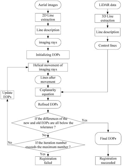
Figure 1.
Steps of the aerial images and LiDAR data registration based on line vectors.
2.1. Line Vector
As shown in Figure 2, the unit direction vector of lines can be expressed by three direction cosines, namely , which satisfies , i.e., , but these three parameters cannot determine the position of the line. The position vector of H, an arbitrary point on the line directed by the origin is r, according to which the position of the line can be determined and line vector L can be obtained. Line vector L is a six-vector, including the primary part and secondary part. The directional vector is the primary part of the line vector, while the moment vector is the secondary part of the line vector. The directional vector does not change as the origin changes, but the moment vector does. For this reason, we know that the line vector is a vector attached to a line in the space and six-dimensional linear space in the real number field:
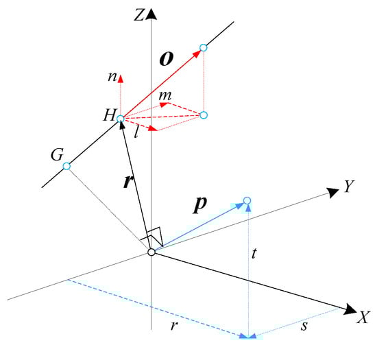
Figure 2.
Line vector coordinate of lines.
The directional vector and moment vector satisfy: . According to the two constraints that and , which derive from the unit line vector itself, there are four degrees of freedom in the line vector coordinate.
Assume there are two line vectors L1 and L2, which are , . Operations on line vectors are performed similar to those on Cartesian vector, also referred to as line dot- and cross-products [17], and are defined by:
The advantage of the linear expression method based on line vector coordinate is in determining a line not relying on any point or surface, as well as directly representing a line direction by using a directional vector and line position by a moment vector.
Assuming any two lines with their directional vectors set as and , respectively, and their moment vectors as and , respectively, if these two lines are coplanar, then they will meet the requirement of:
Equation (4) is the coplanar formula of the two lines in a simple way. Compared with the two traditional methods of using point coordinates and the orientation vector to express the coplanar formula, the line vector may directly make use of the information of direction and position.
2.2. The Coordinate Transformation of Line Vectors
As shown in Figure 3, hg is an image feature line passing through point h and point g. Imaging ray Sh from the photographing center S runs through point h and Sg runs through point g. As a corresponding control line in LiDAR data, GH runs through point G and H. In regard to lines Sh, Sg, and GH, assume their directional vectors of are , , and O, moment vectors are , , and P, and all three lines are coplanar at photographing, then, based on Equation (4), the LiDAR data coordinate system and the image coordinate system have the following relation:
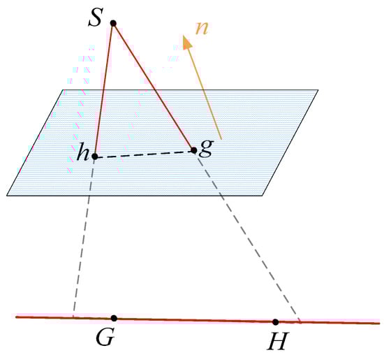
Figure 3.
Coplanar model based on line vectors.
In the aforesaid equation, the coordinate transformation relationship between the LiDAR data coordinate system and the image coordinate system is characterized by representing coordinates of g and h in the image coordinate system, as well as coordinates of G and H in the LiDAR coordinate system. Any two LiDAR points can determine control lines and two image points can determine corresponding image lines, so g and h, as well as G and H, are not required to be corresponding points, which is the advantage of registration using line characteristics.
Directional vectors and moment vectors of imaging rays cannot make Equation (5) workable because there are certain deviations of the original position and direction of the photographing center. Such a photographing center should be moved to restore the correct position and direction of Sh and Sg. That is to say, Sh and Sg should be carried out of the coordinate transformation to meet Equation (5). The coordinate transformation of the line vector is generally achieved by a dual quaternion. Line can be obtained from L by the dual quaternion, q:
where , , , and is the conjugation of q.
2.3. Coplanarity Equation Based on Line Vectors
Assuming the original line vector coordinate of the imaging ray Sh is (l1, m1, n1, r1, s1, t1). Then the line vector coordinates of Sh through coordinate transformation can be obtained by Equation (6):
Similarly, line vector coordinates of Sg through coordinate transformation can be obtained by its original line vector coordinate (l2, m2, n2, r2, s2, t2). Assuming the line vector coordinate of GH is (L, M, N, R, S, T), wherein O = (L, M, N) and P = (R, S, T). The coplanarity equation based on line vectors can be expanded by substituting the line vector coordinates of Sh, Sg, and GH into Equation (5). Sh, Sg, and GH are coplanar when Sh and Sg obtain the correct position and direction by correcting the attitude and position of S. Hence, the key of line vector registration is to solve the EOPs represented by the dual quaternion q.
2.4. Practical Procedure of Solving the Problem
The proposed adjustment mode includes the following five parts, and all the data are associated automatically:
Representation of a Straight Line
The unit line vector coordinate constituted by any two points G (XG, YG, ZG) and H (XH, YH, ZH) of a control line in the LiDAR data coordinate system is [19]:
Similarly, line vectors can be used to express two imaging rays Sh and Sg.
Determination of Initial Values
We can determine the original values of the unknown values q by inputting rotation parameters ω, φ, κ, and translation parameters XL, XL, XL into Equation (9):
Establishment of the Error Equation
For the least-squares adjustment, the coplanarity equations (Equation (5)) are linearized in the form:
where the observations are the image coordinate measurements, and the unknowns are the registration parameters described by X. V are the correction values of the observed values. F are the residual terms of the observed values, which are obtained by putting the approximate value of the unknown value on the left-hand side of Equation (5). A are the coefficient terms of the error equation.
3. Results
3.1. Testing Methods
Three datasets of corresponding lines from the synthetic, ISPRS test project, and real image are adopted for experiments. The synthetic image is adopted to verify the correctness of the proposed algorithm, and the ISPRS test project image and real image are adopted to verify the practicability of the proposed algorithm. Conventional registration and the proposed registration method based on line vectors are performed in each type of image. The initial set of unknowns in conventional registration is , while the LVR gives data of q1 = 1, q2 = q3 = q4 = q01 = q02 = q03 = q04 = 0, equivalent to the initial set in conventional registration. A description of each dataset is described below.
(1) Synthetic images: The generation method of synthetic data is as follows: firstly a parameter distortion model (PDM) is used in the camera calibration with radial distortion and decentering distortion included. Then the accurate camera inner orientation parameters (IOPs) and the EOPs of each image are obtained. Substituting the ground control points, camera parameters, and the EOPs of the image into the collinear equation, the coordinates of corresponding points can then be calculated. Finally, the IOPs and the corresponding points in the image and LiDAR data coordinate framework are used as the given data to solve the EOPs, since there may be some random errors in the measurement of point coordinates in practical applications. To simulate the actual situation, we using the Gaussian random function to produce Gaussian errors with zero-mean and 1.0 pixel standard deviation based on simulated data, assign these data in the x-axis and y-axis of 18 endpoints of image lines, wherein random errors on the x-axis and y-axis are required to be, respectively, generated to ensure their independence. The IOPs of the synthetic image have a principal point of x0 = 0, y0 = 0 and a principal distance of f = 28 mm. The image format was 1024 × 1280 with a pixel size of 0.008 mm.
(2) ISPRS test project data: A group of data is a subset of the ISPRS test project on Urban Classification and 3D Building Reconstruction. Everyone can download it from the ISPRS website. The study area is located in Vaihingen City. Aerial images are shot by a digital mapping camera (DMC), wherein the focal length of DMC is 120 mm, the charge-coupled device (CCD) pixel size is 12 μm ground resolution of images and the frame of image is 7680 × 13,824. LiDAR point clouds are collected by the Leica ALS50 subminiature LiDAR with a density of the point clouds of 6.7 point/m2.
(3) Real aerial imagery and airborne LiDAR data: The study area is located at the University of Calgary. Aerial imagery is shot by Phase One, wherein the focal length of DMC is 60.6785 mm, the CCD pixel is 6 μm ground resolution of images and the frame of image is 6732 × 8984. The density of the point clouds is 3.5 point/m2.
For each dataset, a single image is selected for registration with the LiDAR data. The image lines and LiDAR lines were manually measured. A set of nine evenly-distributed control lines were manually selected for each dataset, while others were used as check lines. Figure 4 shows the distributed control lines for the ISPRS test project, and the real image, respectively. Yellow lines are used to represent control lines and green lines are used to represent check lines.
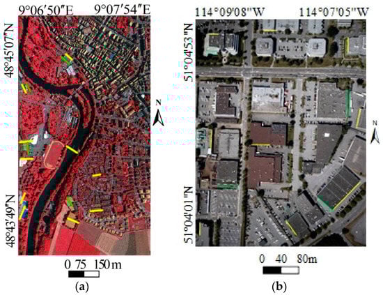
Figure 4.
Distribution of (a) simulated and (b) ISPRS test project.
3.2. Experimental Results
The accuracy of registration consists of theoretical accuracy and real accuracy [23]. The standard error of unit weight () of least squares adjustment is used to estimate the theoretical accuracy of the line vector registration. Theoretical accuracy of unknowns is shown in Table 1. To quantitatively verify the real accuracy of line vector registration, we used the root mean square error (RMSE) of the check line, which is calculated by projecting two arbitrary points of each LiDAR check line onto the image using solved EOPs and then calculating the mean distances from projected points to their corresponding image lines. The errors for check lines of conventional registration and LVR methods are listed in Table 2.

Table 1.
Registration results of simulated, ISPRS test project, and real images.
Table 2.
RMSE of check lines of conventional registration and LVR (pixel).
Figure 5 represents the effect on the image before and after registration. We extract the point cloud of building roofs in LiDAR data, and project the roof point cloud onto the image by the solved EOPs, where projected roof points are shown in blue. Figure 6 represents the whole and the local 3D effects of the images after registration. Since the LiDAR was pointing vertically down, the points only distribute on the roof of the building, without any distribution on the facade, and the color of the building facade is black after registration.
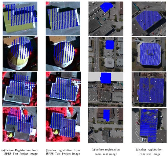
Figure 5.
Registration effects of the image.
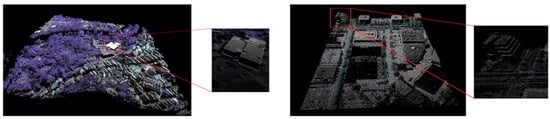
Figure 6.
3D display of the registration effects.
4. Discussion
The registration of aerial images and airborne LiDAR data based on linear features are merely methods based on points or establishing a registration model using line direction. The coplanarity equation of the line vector is established by coplaning two imaging rays and the corresponding control lines. A registration method using line vectors is raised to solve the traditional weak geometric constraint.
Experimental results show that both conventional registration and LVR can achieve the correct solution. When handing synthetic data, position error of EOPs from both conventional registration and LVR method is within 0.84 m and an attitude error of EOPs is within 0.00466°. Compared with conventional registration, LVR has 18% higher accuracy in the position parameter and 14% higher accuracy in the attitude parameter. Additionally, the averaged error of check lines by conventional registration is 1.07 pixels, while with the LVR method it is 0.88 pixels. Compared with conventional registration, the LVR method is 18% better in real accuracy. When handling ISPRS test project data, the EOPs are estimated with a value of 2.00 pixels via conventional registration, and the RMSE of the check lines at the image scale is 0.66 pixels. In contrast, a value of 1.75 pixels is achieved for the LVR, with the RMSE of the check line being 0.54 pixels. When handling real aerial images in Calgary, the LVR is about 20% higher and 24% higher than conventional registration in theoretical accuracy and real accuracy, respectively.
The proposed adjustment is evaluated by a synthetic, ISPRS test project and real data. Compared with the traditional method, the LVR is theoretically and actually more accurate. This is because conventional registration only uses the direction of the line to set up the registration model, whose essence is still the coplanarity of points. The LVR uses directional and moment vectors to describe feature lines, covering both the direction and position information of the lines.
The inaccurate original EOPs before registration has resulted in large deviation in real roof positions and projecting points on the image. The registration of real roof positions and projecting points on an image has been accurately achieved after the registration of aerial images and LiDAR data. It follows that the LVR can achieve an ideal registration accuracy in urban areas with rich linear features.
There are some limitations in the proposed algorithm, though the imaging rays in the image coordinate framework and their corresponding linear control features in LiDAR data coordinate framework can be effectively achieved by line vectors. The raised method achieves accurate extraction of line features by selecting points on aerial images and LiDAR for plan fitting and then plane intersection. Point features selected artificially are assumed on the same plane, so it is actually difficult to ensure that all these points are on the building surface. The contingency may occur in coplanar features as selected points cannot represent the coplanar constraint conditions.
5. Conclusions
In this paper, we have proposed a new algorithm that uses line vectors to represent imaging rays and control lines. Moreover, it breaks the limitation of the traditional “four-point” coplanar condition by directly describing the “three-line” coplanar condition. The geometrical meaning of the proposed model for the registration becomes more explicit.
According to this study, straight lines are proven to be reliable and effective in registration, and points in the image coordinate framework and LiDAR data coordinate framework on the lines are not necessarily correspondent. To reduce the contingency in extracting line features, further research will be focused on directly using plane features for registration of aerial image and LiDAR data.
Acknowledgments
This work was supported in part by the National Natural Science Foundation of China under grant 41471381, the Natural Science Foundation of Jiangsu Province of China under grant BK20171410, and the Open Research Fund of State Key Laboratory of Tianjin Key Laboratory of Intelligent Information Processing in Remote Sensing under grant 2016-ZW-KFJJ-01. Heartfelt thanks are also given for the comments and contributions of anonymous reviewers and members of the editorial team.
Author Contributions
Qinghong Sheng, Qi Wang, and Bin Zhang conceived and designed the experiments. Xinyue Zhang performed the experiments. Bo Wang and Qi Wang analyzed the data. Qinghong Sheng and Zhengning Zhang wrote the paper.
Conflicts of Interest
The authors declare no conflict of interest.
References
- Axelsson, P. Processing of Laser Scanner Data-algorithms and Applications. ISPRS J. Photogramm. Remote Sens. 1999, 54, 138–147. [Google Scholar] [CrossRef]
- Baltsavias, E.P. A Comparison between Photogrammetry and Laser Scanning. ISPRS J. Photogramm. Remote Sens. 1999, 54, 83–94. [Google Scholar] [CrossRef]
- Palenichka, R.M.; Zaremba, M.B. Automatic extraction of control points for the registration of optical satellite and LiDAR images. IEEE Trans. Geosci. Remote Sens. 2010, 48, 2864–2879. [Google Scholar] [CrossRef]
- Cheng, L.; Tong, L.; Chen, Y.; Zhang, W.; Shan, J.; Liu, Y.; Li, M. Integration of LiDAR Data and Optical Multi-view Images for 3D Reconstruction of Building Roofs. Opt. Lasers Eng. 2013, 51, 493–502. [Google Scholar] [CrossRef]
- Cheng, L.; Gong, J.; Li, M.; Liu, Y. 3D building model reconstruction from multi-view aerial imagery and lidar data. Photogramm. Eng. Remote Sens. 2011, 77, 125–139. [Google Scholar] [CrossRef]
- Chen, L.; Hoang, D.; Lin, H.; Nguyen, T. Innovative Methodology for Multi-View Point Cloud Registration in Robotic 3D Object Scanning and Reconstruction. Appl. Sci. 2016, 6, 132. [Google Scholar] [CrossRef]
- Gunay, A.; Arefi, H.; Hahn, H. Semi-automatic true orthophoto production by using LIDAR data. In Proceedings of the IEEE International Geoscience and Remote Sensing Symposium, Barcelona, Spain, 23–28 July 2007; pp. 2873–2876. [Google Scholar]
- Kanaev, A.V.; Daniel, B.J.; Neumann, J.G.; Kim, A.M.; Lee, K.R. Object Level HSI-LIDAR Data Fusion for Automated Detection of Difficult Targets. Opt. Express 2011, 19, 20916–20929. [Google Scholar] [CrossRef] [PubMed]
- Cui, T.; Ji, S.; Shan, J.; Gong, J.; Liu, K. Line-Based Registration of Panoramic Images and LiDAR Point Clouds for Mobile Mapping. Sensors 2017, 17, 70. [Google Scholar] [CrossRef] [PubMed]
- Zhang, Y.; Xiong, X. Automatic registration of urban aerial imagery with airborne LiDAR data. J. Remote Sens. 2012, 16, 579–595. [Google Scholar]
- Rönnholm, P.; Hyyppä, H.; Hyyppä, J.; Haggrén, H. Orientation of Airborne Laser Scanning Point Clouds with Multi-View, Multi-Scale Image Blocks. Sensors 2009, 9, 6008–6027. [Google Scholar] [CrossRef] [PubMed]
- Swart, A.; Broere, J.; Veltkamp, R.; Tan, R. Refined Non-rigid Registration of a Panoramic Image Sequence to a LiDAR Point Cloud. Photogramm. Image Anal. Lect. Notes Comput. Sci. 2010, 6952, 73–84. [Google Scholar]
- Yang, B.; Chen, C. Automatic registration of UAV-borne sequent images and LiDAR data. ISPRS J. Photogramm. Remote Sens. 2015, 101, 262–274. [Google Scholar] [CrossRef]
- Parmehr, E.G.; Fraser, G.S.; Zhang, C.; Leach, J. Automatic registration of optical imagery with statistical similarity 3D LiDAR data using. ISPRS J. Photogramm. Remote Sens. 2014, 88, 28–40. [Google Scholar] [CrossRef]
- Lv, F.; Ren, K. Automatic registration of airborne LiDAR point cloud data and optical imagery depth map based on line and points features. Infrared Phys. Technol. 2015, 71, 457–463. [Google Scholar] [CrossRef]
- Habib, A.; Ghanma, M.; Morgan, M.; Al-Ruzouq, R. Photogrammetric and lidar data registration using linear features. Photogramm. Eng. Remote Sens. 2005, 71, 699–707. [Google Scholar] [CrossRef]
- Zheng, S.; Huang, R.; Zhou, Y. Registration of optical images with lidar data and its accuracy assessment. Photogramm. Eng. Remote Sens. 2013, 79, 731–741. [Google Scholar] [CrossRef]
- Liu, S.; Tong, X.; Chen, J.; Liu, X.; Sun, W.; Xie, H.; Chen, P.; Jin, Y.; Ye, Z. A linear feature-based approach for the registration of unmanned aerial vehicle remotely-sensed images and airborne LiDAR data. Remote Sens. 2016, 8, 82. [Google Scholar] [CrossRef]
- Wang, Y.; Wang, Y.; Wu, K.; Yang, H.; Zhang, H. A dual quaternion-based, closed-form pairwise registration algorithm for point clouds. ISPRS J. Photogramm. Remote Sens. 2014, 94, 63–69. [Google Scholar] [CrossRef]
- Fischer, I. Dual-Number Method in Kinematics, Statics and Dynamics; CRC Press: Boca Raton, FL, USA, 1998. [Google Scholar]
- Rooney, J. A comparison of representations of general spatial screw displacement. Environ. Plan. B Plan. Des. 1978, 5, 45–88. [Google Scholar] [CrossRef]
- Chen, G.; Wang, H.; Lin, Z.; Lai, X. The principal axes decomposition of spatial stiffness matrices. IEEE Trans. Robot. 2015, 31, 191–207. [Google Scholar] [CrossRef]
- Mikhail, E.M.; Bethel, J.S.; McGlone, J.C. Introduction to Modern Photogrammetry; Jhon Wiley & Sons: New York, NY, USA, 2001; pp. 144–146. [Google Scholar]
© 2017 by the authors. Licensee MDPI, Basel, Switzerland. This article is an open access article distributed under the terms and conditions of the Creative Commons Attribution (CC BY) license (http://creativecommons.org/licenses/by/4.0/).