Observation and Simulation of Axle Box Acceleration in the Presence of Rail Weld in High-Speed Railway


1
Key Laboratory of High-Speed Railway Engineering, Ministry of Education, Southwest Jiaotong University, Chengdu 610031, China
2
School of Civil Engineering, Southwest Jiaotong University, Chengdu 610031, China
3
School of Mechanical Engineering, Southwest Jiaotong University, Chengdu 610031, China
*
Authors to whom correspondence should be addressed.
Appl. Sci. 2017, 7(12), 1259; https://doi.org/10.3390/app7121259
Submission received: 17 October 2017
/
Revised: 7 November 2017
/
Accepted: 30 November 2017
/
Published: 4 December 2017
Abstract
:Rail welds are widely used in high-speed railways and short-wave irregularities usually appear due to limitations in welding technology. These irregularities can excite a high wheel/rail force and are regarded as the main cause of deterioration in track structures. To measure this fierce force (or deterioration of the rail weld), axle box acceleration is treated as an effective and economic measure, though an exact quantitative relation between these two quantities remains elusive. This paper aims to develop such a relation in order to provide a new theoretical basis and an analysis method for monitoring and controlling weld geometry irregularity. To better understand the characteristics of axle box acceleration, the paper consists of two parts: an observation and a numerical simulation of axle box acceleration by rail welds. Based on measured data from field tests, axle box acceleration at rail welds was found to have high-frequency vibrations in two frequency bands (i.e., 350–500 Hz and 1000–1200 Hz). Upon analyzing the vibration characteristics in time–frequency domains, the exact location of the rail weld irregularity could be identified. Subsequently, a 3D high-speed wheel/rail rolling contact finite element model was employed to investigate the effect of rail weld geometry on axle box acceleration, and led to the discovery that the weld length and depth determine the vibration frequency and amplitude of the axle box acceleration, respectively. A quantitative relation between axle box acceleration and wheel/rail force has also been determined. Finally, we propose an approach for real-time health detection of rail welds and discuss the influence of other defects and rail welds on the acceleration signal of the axle box.
1. Introduction
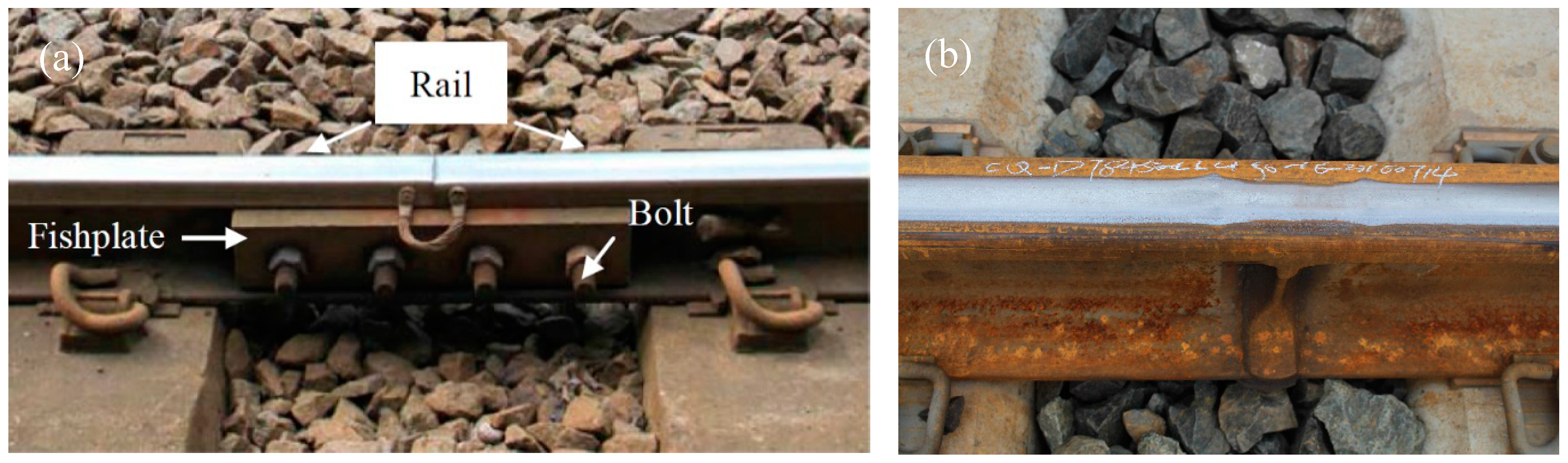
On a traditional railway track, a fishplate and bolt, as shown in Figure 1, are used to join rails [1]. The large dynamic force generated by geometric discontinuities between a wheel and the rail at joint gaps is one of the weak points in track structure. However, as shown in Figure 1, rails of standard length can be welded into rails of extended length, which is one important measure towards eliminating rail joints.
Flash welding and thermite welding are mainly used in rail welding. However, absolute smoothness of the geometric surface of the rail weld cannot be attained due to limitations in welding technology and improper operation, etc. If the temperature of the rail surface and adjacent area is lower than the melting temperature during flash welding, achieving complete contact between the melt and parent metal is hard and crystalline lenses, micro-pores, and non-metallic impurities will appear in the welds during forging [2]. In addition, the strength, hardness, and micro-structure of the welding materials are different from that of the parent metal [3], and unaligned ends of welded rails, inequality of grinding, and welding parts by hand will cause irregularities on the surface of the rail [4]. Gao and Zhai [5] carried out a detailed survey on geometric irregularities at rail welds on high-speed railways in China. They found that a short-wave irregularity with a wavelength range from 0.05 to 0.39 m was the main form. Initiation and development of such an irregularity can be from high-frequency excitation, which finally loses its energy by dissipation in the form of plastic deformation and other processes related to the growth of track damage, as reported by Wen [6], Correa [7], and Mandal and Dhanasekar [8]. Therefore, controlling the size of the short-wave irregularity of welds is of great importance to ensure secure, stable, and economic operation of high-speed railways. Xiao [9] investigated the influence of weld defects with different wavelengths on the wheel/rail force and proposed safety limits under different speeds based on the dynamics index or dynamic factors. Steenbergen and Esveld [10,11] evaluated the quality of rail welds using a geometric gradient, which can be used for considering any geometric form of the weld. Related standards have also been determined on the basis of numerical calculations and engineering experience.
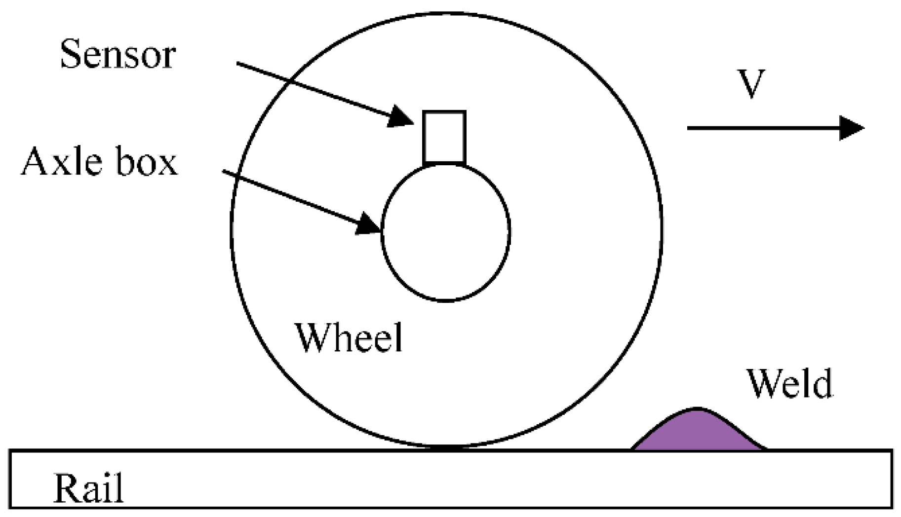
The precondition of carrying out the evaluation of wheel–rail force at rail welds stated in [9,10,11] is to obtain its geometric size, which is definitely time consuming and labor intensive. For effective measurement of irregularities in the tracks, detecting vertical axle box acceleration (hereinafter referred to as ABA) is a simple and economical method. An accelerometer sensor can be easily installed on the axle box (see Figure 2) without limitations of the vehicle’s running speed [12,13]. To reflect on the health condition of track systems, many scholars have, therefore, focused their studies on ABA. Liang [14] developed a set of indoor rolling test devices that was used for simulating the response of ABA under low-speed conditions, which ranged from 3.5 to 15 km/h, when there were defects on the wheel/rail surface. Obvious fluctuations in ABA were generated at the defects that were confirmed via time–frequency technology according to research findings to be damage on the wheels or rails. Molodova and Li [15] carried out a series of ABA tests targeted at monitoring the health of some preliminary damage (e.g., rail squats, rail pad degradation, and fastening cracks) occurring at weld joints on site; the results showed an obvious difference between rail welds that were in good and poor condition. On this basis, Li [16] put forward three approaches to improve the success rate of monitoring. However, the methods are currently applied on lines of ordinary speed (that is, 140 km/h). Zhai’s group [17] conducted abundant tests on high-speed railway lines in China. With obtaining the dynamic response of ABA up to 350 km/h, the results have shown that high-frequency vibration exists in ABA.
The above studies focused mainly on testing ABA. It is difficult to carry out tests under extreme conditions due to many unknown factors in the measured work and due to safety considerations. Consequently, it is vital to develop a numerical model for an in-depth investigation. In the past, problems of dynamics were widely processed by adopting a rigid multi-body dynamics model [18]. Results from the modal analysis introduced to the rigid model are regarded as a way to further consider high-frequency dynamic effects of wheel/rail high-speed rolling contact. However, upon considering the vibration mode, the wheel/rail contact geometry relationship becomes complex and difficult to solve because of the bending and torsion of the wheel/rail systems. In recent years, a new method—the explicit finite element (FE) method—has been used to solve problems of high-frequency wheel/rail rolling contact [6,15,19,20,21,22,23]. This method abandons three basic assumptions including infinite half space, steady rolling, and linear elastic materials of the classic contact algorithms such as Kalker’s CONTACT [22]. Molodova and Li [19,20] developed a 3D explicit FE model based on this method to simulate the change in ABA at short-wave irregularities of rail at a speed of 140 km/h; their results agreed with that of the test site. It should be noted that Molodova and Li’s main purpose for developing such a model was to monitor squat defects on the rail surface and the degrees of damage. Therefore, the relationship between ABA and wheel/rail force was not given and we cannot estimate degradation of the defect through ABA as the evaluation index is always wheel/rail force or geometry size.
The operating speeds of high-speed railway in China have reached 300 km/h, bringing higher requirements for safety. This paper aims to provide a new theoretical basis and analysis method to monitor and control welds at at such high speeds. First, the S transform was used to analyze vibration characteristics of ABA in the time–frequency domain at welds based on the measured data of 300 km/h. Then, a validated 3D wheel/rail rolling contact FE model was employed to simulate dynamic responses of ABA induced by rail welds under 300 km/h through investigating the influence of weld geometry on ABA. A quantitative relationship between ABA and wheel/rail force has also been established. Based on these results, an approach to estimate rail weld is proposed. The differences in ABA induced by rail weld, rail corrugation, and wheel flat are then discussed.
2. Observation of Time–Frequency Vibration of the Measured Axle Box Acceleration
High-frequency contact vibration generated on the wheel/rail surface under excitation of all kinds of irregularities can be easily transferred to the axle box due to large contact stiffness between wheel and rail. A trial measurement at a speed of 300 km/h on a certain Chinese high-speed railway was conducted by the State Key Laboratory of Traction Power of Southwest Jiaotong University. The track is non-ballast track containing rail, fastening, slab, and mortar and the car was CRH380. The ABA measurement (four accelerometer sensors) was installed on the axle box of a bogie (see Figure 3). The data acquisition unit was connected with the sensor mounted on the tested components of the vehicle. The sampling frequency of the axle box acceleration sensor was set to 16.4 kHz.
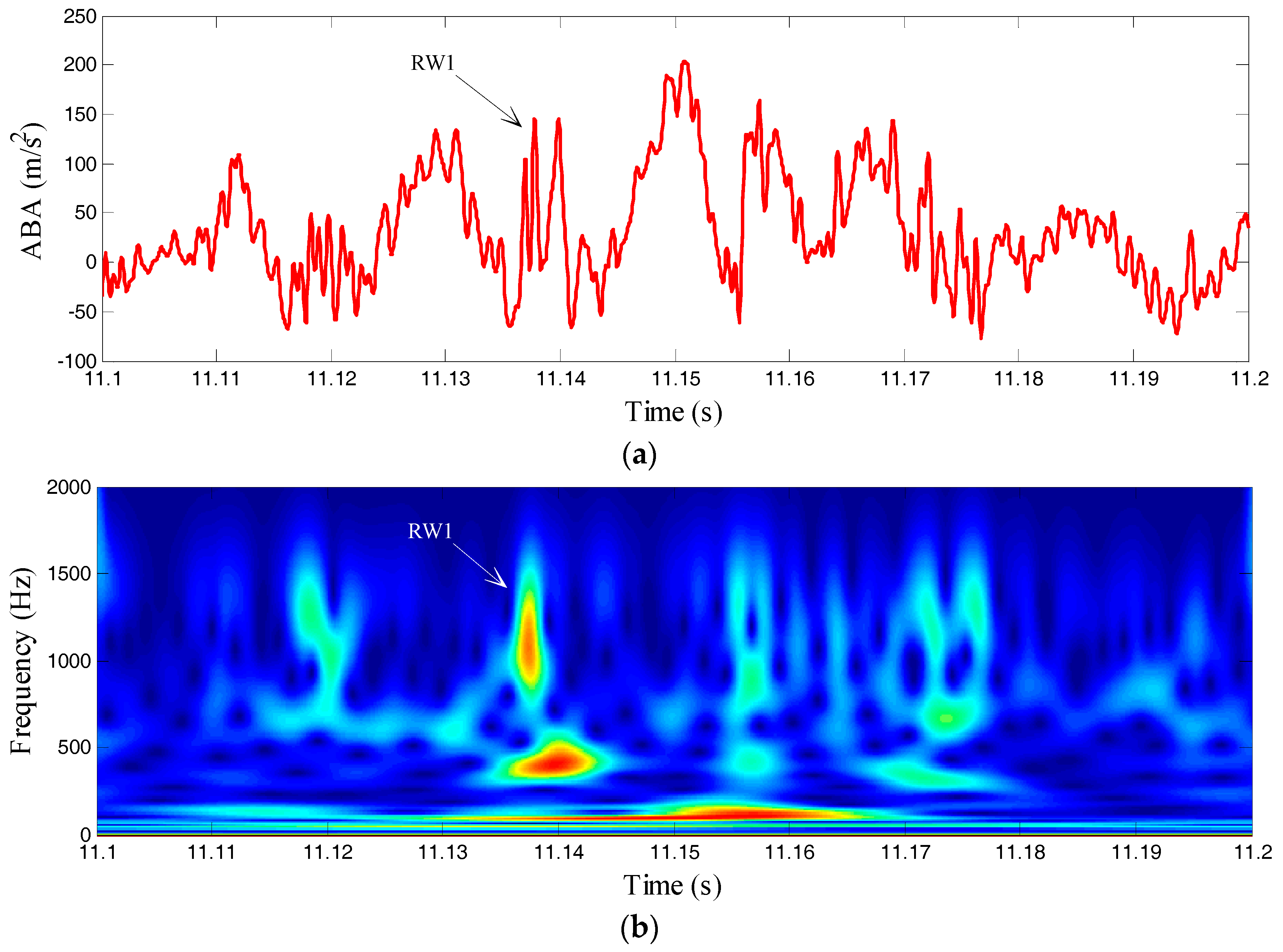
Figure 4 shows the measured ABA changing along with the running time. Note that a 1500 Hz LPF (low pass filter) has been imposed on the signals with consideration of typical frequency range of wheel/rail interaction and noises containing high-frequency signals. The ABA amplitude fluctuated within the range of ±50 m/s2 under 300 km/h on account of geometry irregularities on the surface and elastic deformation of the wheel/rail contact interface. Rails of non-ballast tracks are welded every 100 m. Short-wave irregularities occurred easily in the welds as mentioned in the introduction, and a pulse impulsion occurs every 1.2 s (it is about 100 m as multiplied by the speed of 300 km/h) in Figure 4, whose amplitude reaches 150 to 200 m/s2, as shown in RW1. By contrast, the amplitude at RW2 is rather gentle, possibly because there were no serious irregularities.
To obtain a more detailed analysis and display the vibration of the ABA signal in the time–frequency domain (i.e., the changes of frequency components of acceleration at different times during the process of a vehicle passing the weld), the S transform method was used. This method was selected because it inherits and develops localized ideas of continuous wavelet transform and short-time Fourier transform, and adopts a time window of Gaussian function that presents a good resolution in the time and frequency domains [24]. The S transform can be described by Equations (1) and (2):
where f is frequency; is the Gaussian window function; is a parameter controlling the Gaussian window in a position of time t.
Time–frequency vibration characteristics of the ABA at rail welds are presented in Figure 5 by taking RW1 in Figure 4 as an example. Figure 5a shows the time-domain variation of the ABA between 11.1 and 11.2 s. As we can see, an obvious impact was generated with a high-frequency vibration when passing RW1. The time–frequency dynamic response through the S transform is presented in Figure 5b; the contour has been normalized and the mean vibration energy changed from small to large in blue and red. By this figure, we know that the vibration of ABA at a speed of 300 km/h covers a wide frequency domain. Energy excited by weld geometry irregularity around 11.14 s gathers mainly in two frequency bands: from 350 to 500 Hz and from 1000 to 1200 Hz. High-frequency vibration lasting about 2 to 5 ms is dissipated by the wheel/rail contact interface, which is a major cause of fatigue generation for all kinds of rolling contacts. In addition, the welds excite vibration at a frequency band from 50 to 130 Hz, which reflects the vibration of the bogie and sleeper (the main components of the vehicle–track system). With the long duration, such low-frequency vibration not only transfers to the vehicle but also to the substructure of the track and is an important cause of performance deterioration of infrastructures such as ballast, slabs, and bridges, etc.
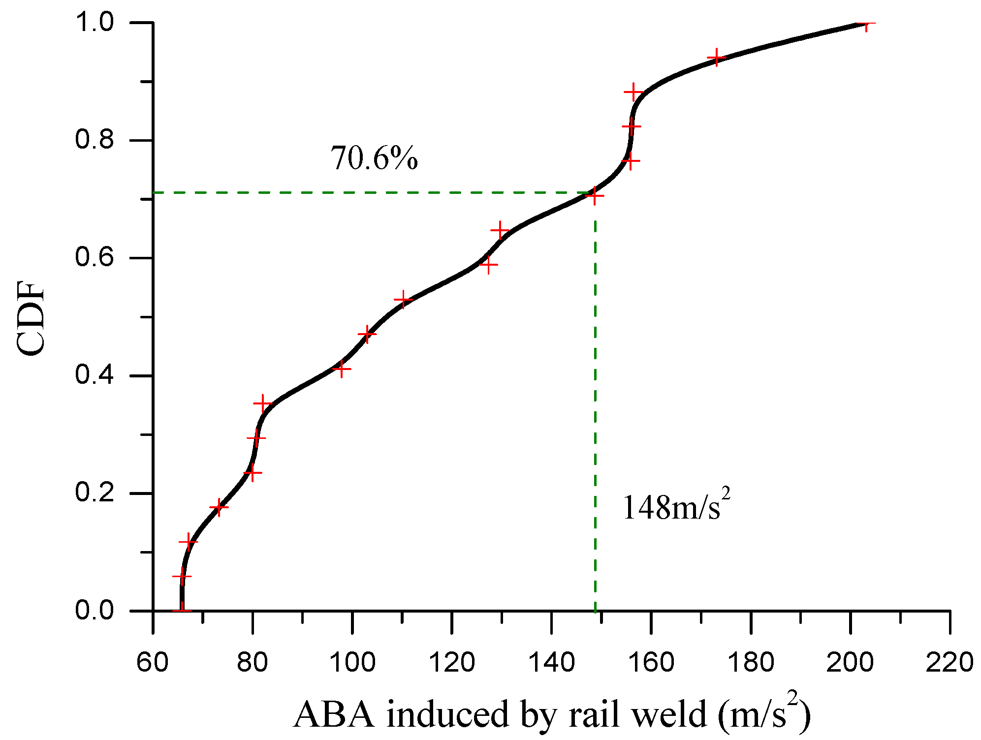
As shown in Figure 4, the signal contains 17 groups of acceleration responses of the axle box at rail welds. CDF (cumulative distribution function) has been used to create statistics on the amplitude of axle box acceleration at these rail welds, as shown in Figure 6. It is obvious that the 17 groups of axle box accelerations change between 66 and 200 m/s2 with nearly 70.6% of the ABAs less than 148 m/s2.
Rail welds have been maintained mainly by limiting the geometry to reduce the wheel/rail force [25]. However, general testing of weld geometry is labor intensive, demanding on resources, and time consuming. To the authors’ best knowledge, there are currently no efficient techniques to measure wheel/rail force, especially for high-speed situations. Therefore, clearly mapping the relationship between ABA data and geometric size of the weld, as well as the wheel/rail force, can help railway departments assess weld geometry from numerous data of ABA, which will improve the efficiency of maintaining the railway system.
3. 3D High-Speed Wheel/Rail Rolling Contact Finite Element Model
3.1. Overview of the Finite Element Model
Figure 7 shows a 3D high-speed wheel/rail rolling contact finite element (FE) model and simulates a vehicle–track system on the high-speed railway line. Only half of a wheelset and track are simulated since the relative longitudinal and vertical planes of a vehicle–track system are symmetric. All components above the primary suspension of a vehicle are simplified as mass points and connected with wheels through the primary suspension. The high-frequency feature between the wheelset and track was fully considered through 3D modeling. It can be approximately assumed that the acceleration of the outer end of the wheel axle is consistent with that of the axle box. The track is a non-ballast track, which was modeled with consideration of the rails, fasteners, slab, and cement asphalt (CA) mortar. The fastening system contains support stiffness and damping that are relevant to the dynamic behavior. The track length of 15.6 m was considered in the model to eliminate the influence of boundary conditions.
The 3D wheelset and rail in real geometry were meshed by an 8-node hexahedral element. The rail was the CHN60 model with the rail cant set as 1:40. “Face-to-face” contact algorithm simulation based on the penalty function method was used for solving contact behaviors among rails. A non-uniform grid was used when meshing the wheel and rail in order to reduce the calculation time without losing precision in the solution. The finest contact zone (element size was 1 mm) was used for solving wheel/rail contact; the farther the contact zone, the larger the grid. The track slab and CA mortar were also stimulated by the 8-node hexahedral elements. The primary suspension and rail fastener of the vehicle were represented by a distributed spring and damping unit. The total number of nodes and elements were 1.46 and 1.29 M, respectively.
The parameters of the model are listed in Table 1. Taking into account the elastic shakedown response of the wheel and rail’s material in the field, a linear elastic material model was used for the wheel and the rail, though more accurate material models can be easily introduced. For an effective computation, the slab and mortar materials were also assumed to be linear elastic.
3.2. Rail Weld in 3D
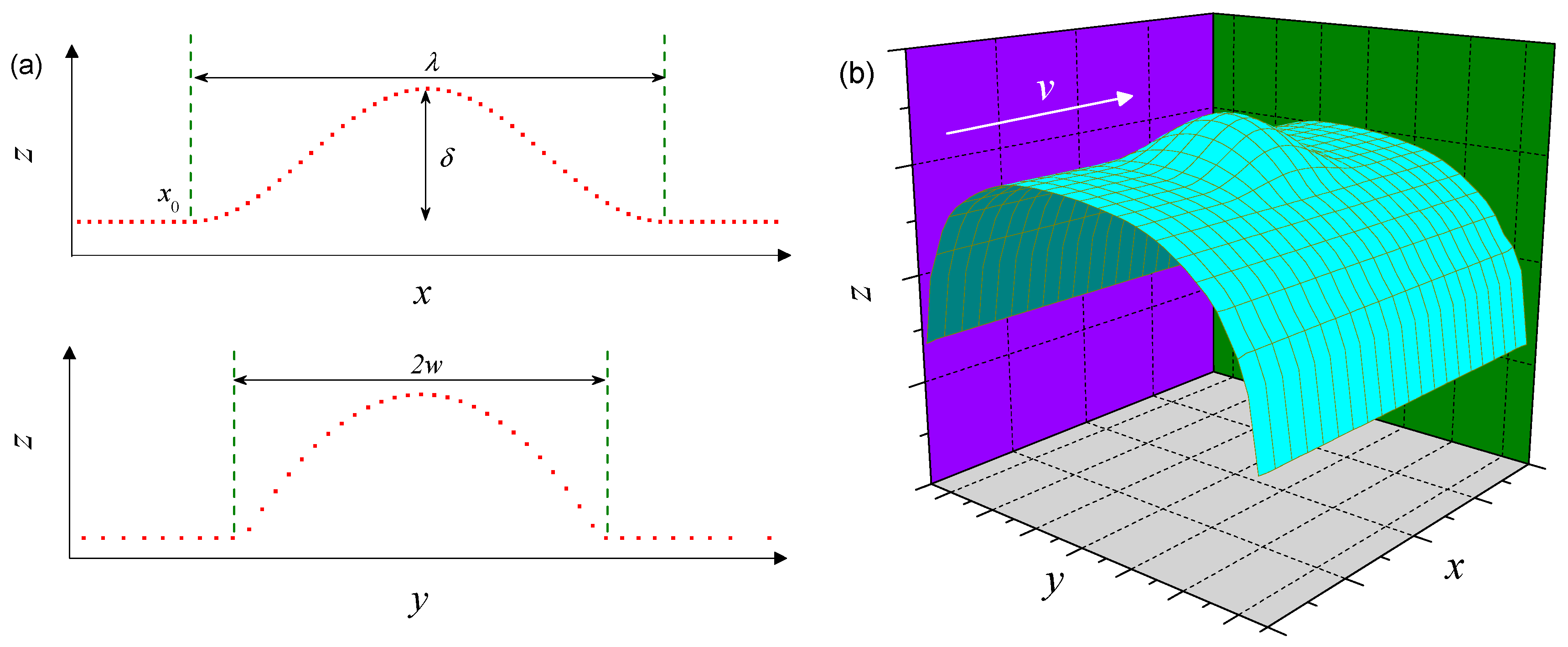
With a smooth wheel/rail surface upon mesh generation, the form of 3D geometry irregularity at rail welds in the calculated area was applied by modifying the coordinates of related nodes on the rail surface by a self-compiled program. For easy understanding, a 3D right-handed Cartesian coordinate system is defined, of which the origin O is located at the initial position of the contact patch (i.e., position A as shown in Figure 7a). The x-axis is defined along the rolling direction and the y- and z-axes are in the lateral and vertical directions. The rail weld model used in this paper for the calculations is shown in Figure 8. Depth (or thickness) D at any element of the simulated weld is cosine in the direction of x and expressed in Equation (3):
For any x within the welding zone, D is parabolic in the y direction,
where and represent wavelength and maximum depth of a rail weld, respectively; is the starting position of a rail weld applied; is one-half width of the weld and assumed as 15 mm in this paper according to field observations.
3.3. Simulation Process
The explicit integral has been widely applied in the solution of the high-frequency phenomenon due to its small time step (the integration time step for the model in this paper was s). Implicit–explicit analysis was adopted in the simulation in order to smooth the dynamic interaction of the wheel and rail by reducing the excitation of the initial energy in the rolling process. Figure 9 shows a schematic diagram of the simulation process; positions A and B are the same as that of Figure 7a. It firstly adopts an implicit algorithm to solve the static contact in the initial position of the wheel, and then it initializes the explicit rolling contact calculation with the vehicle rolling forwards at a constant angular and forward speed v and driven by a constant traction coefficient . The traction coefficient defined by Equation (5) is 0.15 for a typical traction scenario and the friction coefficient is 0.5 for a typical dry wheel–rail contact situation. Note that no force is applied in the lateral direction.
where is the normal load and is the traction force transmitted in the longitudinal direction.
Zone AB between the initial position A and position B is designed to ensure that the wheel achieves steady rolling contact before entering the welding zone (after B). Boundary conditions imposed by the model include constraint of lateral movement on the front of the wheel axle, the longitudinal front end of rails imposed by the longitudinal restraint, the fixed bottom of CA mortar, and primary suspension and fastening reserving only the vertical degree of freedom. More details about the model are referred to in a previous study [22].
4. Results and Discussion
4.1. The Influence of Rail Weld Geometry on ABA
Time-course changes of ABA excited by rail welds with different wavelengths on a high-speed railway line (300 km/h) are presented in Figure 10a. The data has been processed by a 1500 Hz LPF and conforms to the measured data shown in Figure 4. Considering the typical size of the measured weld geometry [5] and the features of short wavelengths concerned in the paper, the wave depth was assumed as 0.2 mm and three wavelengths including 0.05 m, 0.1 m, and 0.2 m were selected. Taking as an example the working condition at a wavelength of 0.05 m, the acceleration of the axle box fluctuated within ±20 m/s2 as a result of elastic deformation between the wheel and rail. This value is less than the measured data (±50 m/s2, see Figure 4) due to the geometry irregularities of the actual line not being considered. When passing the rail weld, it excites strong vibrations of ABA. The first wave crest ABAF was reached at 204.6 m/s2 and was caused by the impact of the rail weld. The continuous fluctuation depends on coupled vibration of the vehicle–track system with a vibration wavelength of 72 mm. It can be observed that ABAV is significantly higher than the first wave crest excited by the rail weld. The phenomena can be found in the measured data of RW1 in Figure 5a.
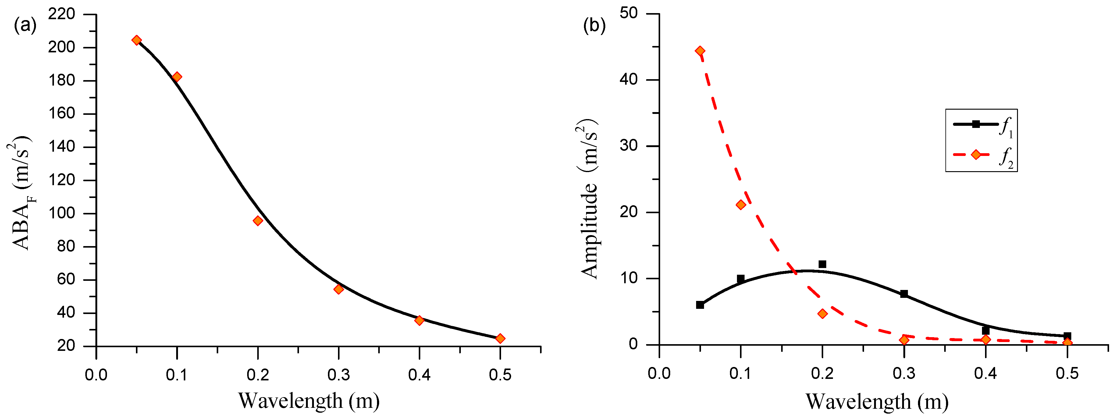
The ABAF decreased from 204.6 m/s2 to 102.4 m/s2 when the wavelength increased from 0.05 to 0.2 m. When the wavelength was 0.2 m, the resonance wavelength (238 mm) caused by the vehicle–track system was significantly greater than that of 0.05 m and 0.1 m. This is because rail welds with long wavelengths do not easily excite high-frequency vibrations in vehicle–track systems, as shown in Figure 10b. This figure shows the distribution of three signals in the frequency domain. There were two obvious dominant frequencies: 350 Hz and 1150 Hz marked as f1 and f2. The two frequencies corresponding to the wavelengths of 238 mm and 72 mm at a running speed of 300 km/h agree with the vibration wavelength shown in Figure 10a.
The variations of ABA under more wavelengths are presented in Figure 11. Figure 11a indicates that ABAF decreased accordingly from 204.6 m/s2 to 24.7 m/s2 with increasing wavelengths from 0.05 m to 0.5 m. In Figure 11b, a corresponding amplitude of ABA at frequency f1 first increased and then decreased along with an increment of the wavelength, reaching a peak at 0.2 m. By contrast, the amplitude at f2 decreased continuously. When the wavelength reached 0.3 m, no dynamic response at f2 was excited. Note that f2 corresponding to vibration wavelengths of 72 mm and 65~80 mm are typical wavelengths of high-speed rail corrugations. Therefore, keeping the wavelength of a rail weld irregularity to no less than 0.3 m can help prevent the occurrence of short-wave rail corrugations, which might also explain why rail corrugations only appeared in certain sections of lines.
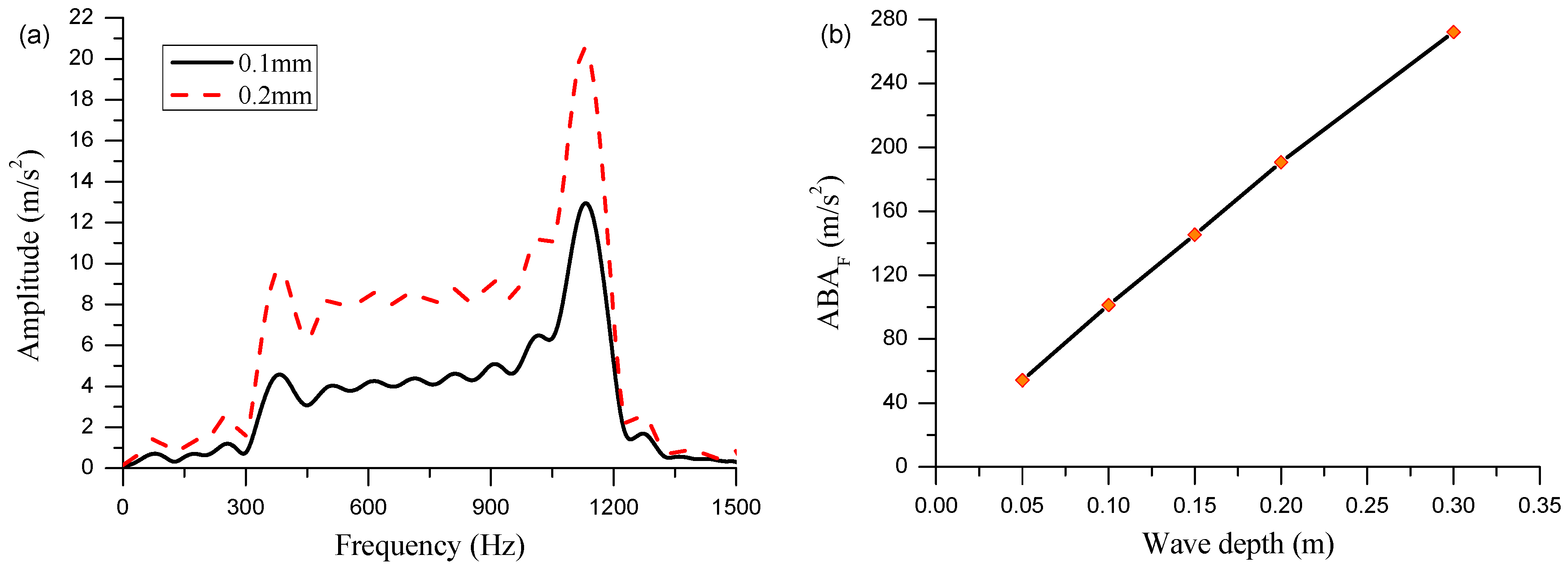
Wave depth is another important parameter of rail weld irregularities, and was also calculated here to know its influence on ABA; a typical wavelength was considered as 0.1 m. The frequency-domain responses of ABA under wave depths of 0.1 and 0.2 mm are presented in Figure 12a. It can be seen that the wave depth affects only the amplitude of ABA but with identical frequency under different wave depths. Thereby, ABAF in Figure 12b grows almost linearly when the wave depth increased from 54.3 m/s2 to 272.1 m/s2.
4.2. The Relationship between ABA and Wheel/Rail Force
Time-course changes of variation of dynamic wheel/rail force Fdyn (the difference between the wheel/rail force and the static wheel load) of the three rail welds in Figure 10a are presented in Figure 13. When the wheel passed over the rail welds, Fdyn initially increased to a peak and then decayed gradually to complete the impact; the amplitude of Fdyn fluctuation was small once leaving the rail weld. By comparing to Figure 10a, it is easy to discover that the rail weld can excite only one impact of the wheel/rail force, but it can induce continuous fluctuations of ABA. The phenomena can be explained by the wheel/rail force that is determined mainly by local geometry irregularity. Thus, no obvious impact action will appear upon passing through the weld. Moreover, continuous fluctuations arise since ABA belongs to the structural vibration with energy that is difficult to dissipate quickly by primary suspension. The maximum of Fdyn will decrease in turn along with the wavelength increase, consistent with the change trend of ABAF.
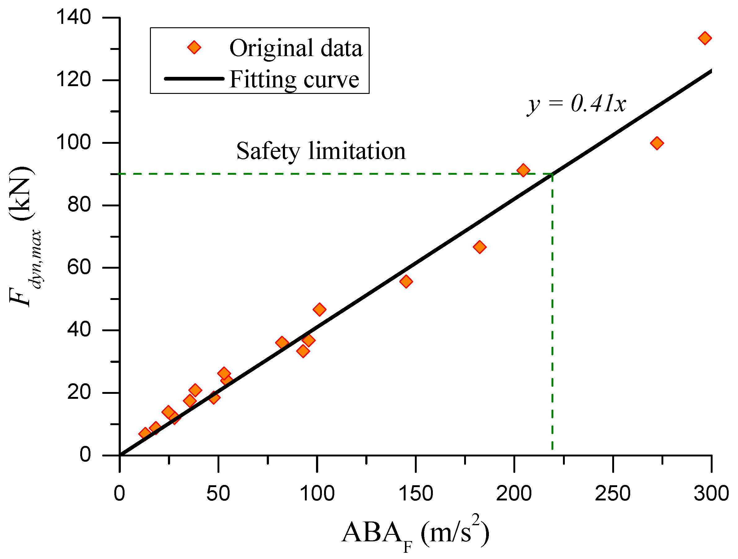
As mentioned above, the first wave crest of ABA at rail welds represents the wheel/rail impact. Eighteen rail welds (including wave depths of 0.1, 0.2, and 0.3 mm that correspond to six wavelengths from 0.05 to 0.5m in Figure 11) were selected for calculation. The relationship between ABAF and maximum of Fdyn (Fdyn,max) has been established, as shown in Figure 14. Discrete points in the figure are the calculation results and the corresponding fitted curve is also shown in the figure; please see Equation (6),
Obviously, a linear relationship is presented between ABAF and Fdyn,max. The measured data in Figure 4 shows that the ABA excited by rail weld irregularities fluctuated within the range of ±50 m/s2 at a vehicle speed of 300 km/h. Thus, the ABA excited by rail welds of long wavelengths or shallow wave depths is submerged, as RW2 in Figure 4. However, a low ABA can mean a small dynamic effect. For instance, the ABA of 50 m/s2 corresponds merely to the Fdyn of 20 kN—far less than the safety threshold—as shown in Figure 14. According to maintenance regulations on Chinese high-speed railways, the Fdyn,max shall be no more than 90 kN; we can find the corresponding threshold value of ABAF to be 220 m/s2. High ABA is easily identified from the measured data, as shown in Figure 4, so that ABA is a good measure for monitoring the health conditions of rail welds. Hence, 17 groups of welds in Figure 6 met the safety threshold. However, a portion of these were within an inch of the danger threshold of 220 m/s2, indicating the need for maintenance as soon as possible.
4.3. Discussion of This Paper
4.3.1. Qualitative Analysis on the Effectiveness of the Model
The FE modeling approach employed in this study originated from Li and Zhao [26]. This approach has been validated by Li and Molodova for high-frequency vehicle–track interaction at squats [19,20], and by Zhao and An for local rolling contact fatigue occurring on high-speed wheel tread [22]. This section tries to further validate it through measured ABA in time and frequency domains. It should be noted that no corresponding weld geometry for measuring ABA in Section 2 was available so only a qualitative analysis will be performed to discuss the effectiveness of the model.
Gao and Zhai [5] indicated that on Chinese high-speed railway lines the average weld geometry irregularity in 0.11 m (0.05~0.39 m) accounted for 78%. Meanwhile, weld straightness should be no more than 0.2 mm for tracks allowing speeds of 300 km/h, according to requirements of maintenance regulations. Therefore, we assumed that geometry wavelength of rail welds corresponding to the measured data in Figure 4 is from 0.05 to 0.4 m with a depth less than 0.2 mm. Figure 5b shows that the wavelength of the rail weld excites two high-frequency vibrations that are well reflected in Figure 10b; similar to the frequency domain response of the 0.2 m wavelength welds. Figure 10a indicates that the wavelength raises the ABA amplitude to about 100 m/s2 in the time domain, less than the measured data (148 m/s2) in Figure 5a. The difference might be caused by the low frequency response generated without the consideration of an actual irregularity in the model built in this paper. For example, a high-energy low-frequency response is seen in Figure 5b, while there is no such response in Figure 10b. It should be emphasized that the results of two measured ABAs in the literature [18] did not overlap completely due to vehicle hunting. In Figure 11a, variations in ABA ranged from 35.6 to 204.6 m/s2 under wavelengths from 0.05 to 0.4 m. It agrees well with the measured data in Figure 6 when we consider that the measured ABA induced by other irregularities is about 50 m/s2. Therefore, the 3D transient finite element model established in Section 3 can effectively simulate the ABA response that is excited by the rail welds.
The effect of differences between actual parameters and model parameters of a vehicle–track system on ABA should be further investigated in the future. These include the change in stiffness of rail pads and fatigue damage of the fastening system [1], the location of the rail weld between the adjacent sleepers [27], existence of track lateral irregularity [28], noise from braking pads, and damage appearance due to an increase in total train mass, etc.
4.3.2. Estimation of Rail Weld Based on ABA Signal Using Time–Frequency Techniques
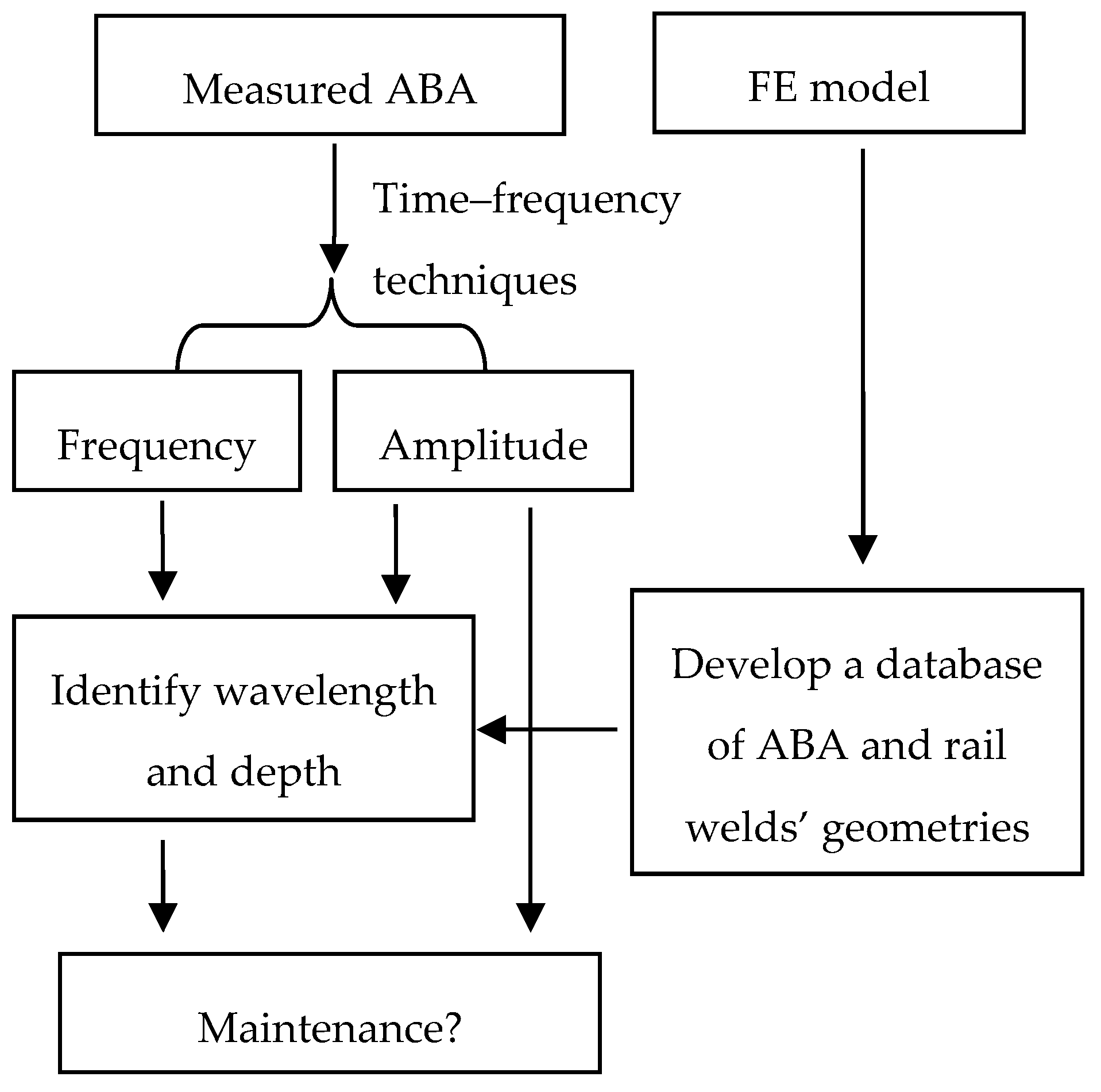
We note that the maximum acceleration of the axle box (202 m/s2) in Figure 5a is not the peak excited by weld RW1, but is the wave crest (148 m/s2) appearing after 11.15 s. In other words, considering merely the maximum amplitude of the ABA in the time domain, the degradation might be overestimated. As the rail weld can excite high frequency vibrations in ABA, which can be found through S transform, we can identify the true location of the rail weld by time–frequency techniques and get corresponding amplitude, as shown in Figure 5. Further, we can estimate the rail weld through a safety limitation (220 m/s2) proposed in Section 4.2. However, a question we should pay more attention to is whether short wavelength irregularity in a rail weld can inspire a higher contact force and increase more rapidly than that of longer wavelengths [9]. Therefore, there is a need to identify the geometries of rail welds.
By parametric analysis in Section 4.1, it can be found that the weld length and depth determine the vibration frequency and amplitude of ABA, respectively. Based on these characteristics, we present an approach for obtaining rail weld geometry from ABA, expressed in Figure 15. Step 1: develop a database of ABA and rail weld geometries through the FE model established in Section 3.1; Step 2: analyze the measured ABA in time and frequency domains using a time–frequency technique, and identify the wavelength and wave depth of the rail weld from the database established in step 1; finally, make a decision whether the rail weld should be maintained. Taking RW1 as an example, it may be 0.1–0.2 m in length as it can excite frequencies of 350 Hz and 1150 Hz shown in Figure 5b and Figure 10b. Further, the true amplitude of ABA by RW1 is 148 m/s2, and we can judge that the wave depth should be about 0.2 mm according to Figure 11a.
4.3.3. Comparison of Other Defects and Rail Weld on ABA
The above results were obtained by assuming that the wheel tread is smooth and that welds only exist on the rail surface; the influence of other flaws in the wheel/rail contact interface was not considered. In fact, a variety of defects such as rail corrugation, wheel polygonal wear, wheel flats, etc., exist in operation, as shown in Figure 16. It is necessary to identify these interfering signals.
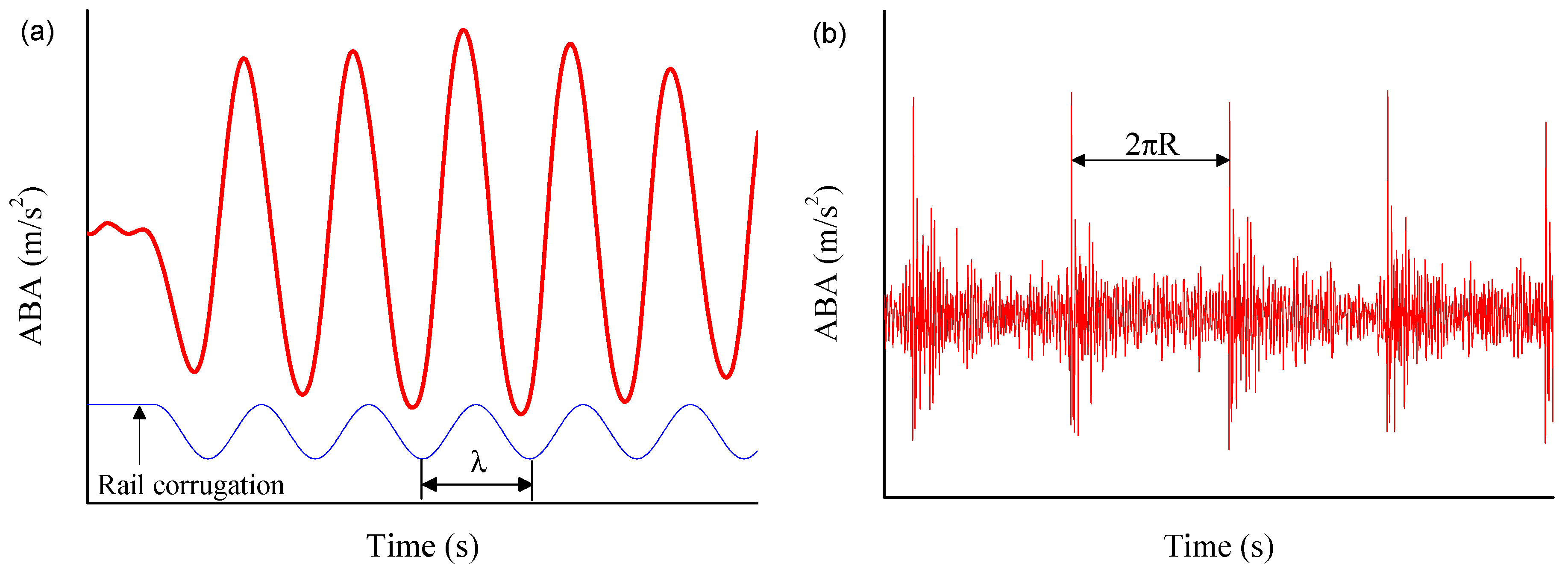
A schematic diagram of ABA induced by rail corrugation and a wheel flat are presented in Figure 17 with horizontal and vertical axes representing the running time and acceleration of the axle box, respectively. As the geometric form of rail corrugation is continuously fluctuating, the excited ABA in corrugation geometric size (a typical size is 65~80 mm) is continued wavelength vibration, as shown in Figure 17a. The vibration mode is different from that in Figure 10a. ABA at welds will gradually decay upon three to four wave crests due to the lack of a continued excitation source, while the rail corrugation can excite longer and with continued fluctuation. Similarly, wheel polygonal wear is continuous with circular geometry fluctuation appearing in the wheel tread. The excited acceleration of the axle box should resemble that of rail corrugation. Thus, the same method can be adopted to identify its influence.
Differing from rail corrugation, wheel flat is a local defect existing in the wheel tread. An impact will be generated on the track system with the wheel rotating every circle. The change in ABA with time is presented in Figure 17b. It can be observed that the distance between two wave crests is the circumference of the wheel. Wheel circumference is generally about 2.7~2.9 m, which is far less than the distance (100 m) of two adjacent rail welds. On the other hand, according to site measurements, the typical wavelength range of the wheel flat in high-speed railways is from 15 to 40 mm, less than the size of a rail weld, which means that a higher ABA can be raised by wheel flats compared to rail welds. So, interference of a wheel flat in the signal of ABA can be identified by the above two differences. To be sure, a more reliable method is to install the acceleration sensors in different wheels to avoid the influence of a flat in a certain wheel.
5. Conclusions
In this paper, the vibration characteristics of an ABA at rail welds in the time–frequency domain have been analyzed at the speed of 300 km/h according to experimental data. A corresponding FE model was developed to simulate ABA and wheel/rail force under different rail welds, which established a quantitative relation between ABA and the wheel/rail force. Based on the results of this study, the following conclusions can be drawn:
- (1)
- According to field tests, the acceleration of an axle box changed within the range of ±50 m/s2 under normal operation, which significantly increased at the welds to amplitudes ranging from 66 to 200 m/s2. High-frequency vibrations at welds existed for a very short time, around 2 to 5 ms. Energy of the high-frequency vibration centralized mainly in two frequency bands: 350 to 500 Hz and 1000 to 1200 Hz.
- (2)
- ABA at rail welds exhibited drastic fluctuations both in measured data and in simulations. The first wave was caused by the impact of the wheel/rail force, while the continued vibration depended on the resonance of the vehicle–track system, for which the amplitude was greater than that generated by the wheel/rail force in certain conditions. Therefore, the maximum value of ABA in the time domain always overestimated the wheel/rail dynamic interaction. To deal with this problem, the position of the rail welds should be determined first by means of time–frequency analysis.
- (3)
- A linear relationship was found between the ABAF and Fdyn,max, and corresponding expressions were established. A value of 220 m/s2 after 1500 Hz LPF can be used as a safety value for real-time onsite monitoring in judging the necessity of maintaining the rail welds.
For a further study, a more detailed database of rail weld geometries and axle box accelerations based on measurements should be established. In addition, simulations should be performed, taking into account the contribution of track stiffness and its variation on ABA, which can be used to detect deterioration of track structure.
Acknowledgments
The present work has been supported by the National Key R & D Plan of China (2016YFC0802203-4), National Natural Science Foundation of China (51425804, 51608459, 51605394 and 51778542) and Doctoral Innovation Fund Program of Southwest Jiaotong University.
Author Contributions
Boyang An and Jinmang Xu conceived and designed the idea and numerical study; Boyang An, Ping Wang, Rong Chen and Dabin Cui analyzed the data and contributed in writing the paper; Ping Wang, Jingmang Xu, Rong Chen and Dabin Cui contributed in obtaining the funding for performing the research.
Conflicts of Interest
The authors declare no conflict of interest.
Abbreviations
The following abbreviations are used in this manuscript:
| ABA | Axle Box Acceleration |
| LPF | Low Frequency Filter |
| CDF | Cumulative Distribution Function |
| 3D | Three Dimensional |
References
- Oregui, M.; Li, S.; Núñez, A.; Li, Z.; Carroll, R.; Dollevoet, R. Monitoring bolt tightness of rail joints using axle box acceleration measurements. Struct. Control Health Monit. 2017, 24, 2. [Google Scholar] [CrossRef]
- Esveld, C. Modern Railway Track; MRT-Productions: Zaltbommel, The Netherlands, 2001. [Google Scholar]
- Mutton, P.; Alvarez, E. Failure modes in aluminothermic rail welds under high axle load conditions. Eng. Fail. Anal. 2004, 11, 151–166. [Google Scholar] [CrossRef]
- Steenbergen, M. Rolling contact fatigue in relation to rail grinding. Wear 2016, 356, 110–121. [Google Scholar] [CrossRef]
- Gao, J.; Zhai, W.; Guo, Y. Wheel–rail dynamic interaction due to rail weld irregularity in high-speed railways. Proc. Inst. Mech. Eng. Part F J. Rail Rapid Transit 2016. [Google Scholar] [CrossRef]
- Wen, Z.; Xiao, G.; Xiao, X.; Jin, X.; Zhu, M. Dynamic vehicle–track interaction and plastic deformation of rail at rail welds. Eng. Fail. Anal. 2009, 16, 1221–1237. [Google Scholar] [CrossRef]
- Correa, N.; Vadillo, E.G.; Santamaria, J.; Herreros, J. A versatile method in the space domain to study short-wave rail undulatory wear caused by rail surface defects. Wear 2016, 352, 196–208. [Google Scholar] [CrossRef]
- Mandal, N.; Dhanasekar, M. Sub-modelling for the ratchetting failure of insulated rail joints. Int. J. Mech. Sci. 2013, 75, 110–122. [Google Scholar] [CrossRef] [Green Version]
- Xiao, G.; Xiao, X.; Guo, J.; Wen, Z.; Jin, X. Track dynamic behavior at rail welds at high speed. Acta Mech. Sin. 2010, 26, 449–465. [Google Scholar] [CrossRef]
- Steenbergen, M.; Esveld, C. Rail weld geometry and assessment concepts. Proc. Inst. Mech. Eng. Part F J. Rail Rapid Transit 2006, 220, 257–271. [Google Scholar] [CrossRef]
- Steenbergen, M.; Esveld, C. Relation between the geometry of rail welds and the dynamic wheel-rail response: Numerical simulations for measured welds. Proc. Inst. Mech. Eng. Part F J. Rail Rapid Transit 2006, 220, 409–423. [Google Scholar] [CrossRef]
- Haigermoser, A.; Luber, B.; Rauh, J.; Gräfe, G. Road and track irregularities: Measurement, assessment and simulation. Veh. Syst. Dyn. 2015, 53, 878–957. [Google Scholar] [CrossRef]
- Grassie, S. Measurement of railhead longitudinal profiles: A comparison of different techniques. Wear 1996, 191, 245–251. [Google Scholar] [CrossRef]
- Liang, B.; Iwnicki, S.; Zhao, Y.; Crosbee, D. Railway wheel-flat and rail surface defect modelling and analysis by time–frequency techniques. Veh. Syst. Dyn. 2013, 51, 1403–1421. [Google Scholar] [CrossRef]
- Molodova, M.; Oregui, M.; Núñez, A.; Li, Z.; Dollevoet, R. Health condition monitoring of insulated joints based on axle box acceleration measurements. Eng. Struct. 2016, 123, 225–235. [Google Scholar] [CrossRef]
- Li, Z.; Molodova, M.; Núñez, A.; Dollevoet, R. Improvements in axle box acceleration measurements for the detection of light squats in railway infrastructure. IEEE Trans. Ind. Electron. 2015, 62, 4385–4397. [Google Scholar] [CrossRef]
- Zhai, W.; Liu, P.; Lin, J.; Wang, K. Experimental investigation on vibration behaviour of a CRH train at speed of 350 km/h. Int. J. Rail Transp. 2015, 3, 1–16. [Google Scholar] [CrossRef]
- Zhai, W. Vehicle–Track Coupling Dynamics, 3rd ed.; Science Publishing House: Beijing, China, 2007. [Google Scholar]
- Molodova, M.; Li, Z.; Dollevoet, R. Axle box acceleration: Measurement and simulation for detection of short track defects. Wear 2011, 271, 349–356. [Google Scholar] [CrossRef]
- Molodova, M.; Li, Z.; Núñez, A.; Dollevoet, R. Validation of a finite element model for axle box acceleration at squats in the high frequency range. Comput. Struct. 2014, 141, 84–93. [Google Scholar] [CrossRef]
- Zong, N.; Dhanasekar, M. Sleeper embedded insulated rail joints for minimising the number of modes of failure. Eng. Fail. Anal. 2017, 76, 27–43. [Google Scholar] [CrossRef]
- Zhao, X.; An, B.; Zhao, X.; Wen, Z.; Jin, X. Local rolling contact fatigue and indentations on high-speed railway wheels: Observations and numerical simulations. Int. J. Fatigue 2017, 103, 5–16. [Google Scholar] [CrossRef]
- Li, S.; Li, Z.; Núñez, A.; Dollevoet, R. New insights into the short pitch corrugation enigma based on 3D-FE coupled dynamic vehicle-track modeling of frictional rolling contact. Appl. Sci. 2017, 7, 807. [Google Scholar] [CrossRef]
- Stockwell, R.; Mansinha, L.; Lowe, R. Localization of the complex spectrum: The S transform. IEEE Trans. Signal Process. 1996, 44, 998–1001. [Google Scholar] [CrossRef]
- Xu, J.; Wang, P.; Gao, Y.; Chen, J.; Chen, R. Geometry evolution of rail weld irregularity and the effect on wheel-rail dynamic interaction in heavy haul railways. Eng. Fail. Anal. 2017, 81, 31–44. [Google Scholar] [CrossRef]
- Li, Z.; Zhao, X.; Dollevoet, R.; Molodova, M. An investigation into the causes of squats—Correlation analysis and numerical modeling. Wear 2008, 265, 1349–1355. [Google Scholar] [CrossRef]
- Askarinejad, H.; Dhanasekar, M.; Cole, C. Assessing the effects of track input on the response of insulated rail joints using field experiments. Proc. Inst. Mech. Eng. Part F J. Rail Rapid Transit 2013, 227, 176–187. [Google Scholar] [CrossRef]
- Zhang, Z.; Dhanasekar, M. Dynamics of railway wagons subjected to braking torques on defective tracks. Veh. Syst. Dyn. 2012, 50, 109–131. [Google Scholar] [CrossRef] [Green Version]
Figure 1.
Rail joint (a) and rail weld (b).

Figure 2.
Installation of the acceleration sensor on the axle box.

Figure 3.
A typical bogie and axle box acceleration (ABA) measurement on an axle box.
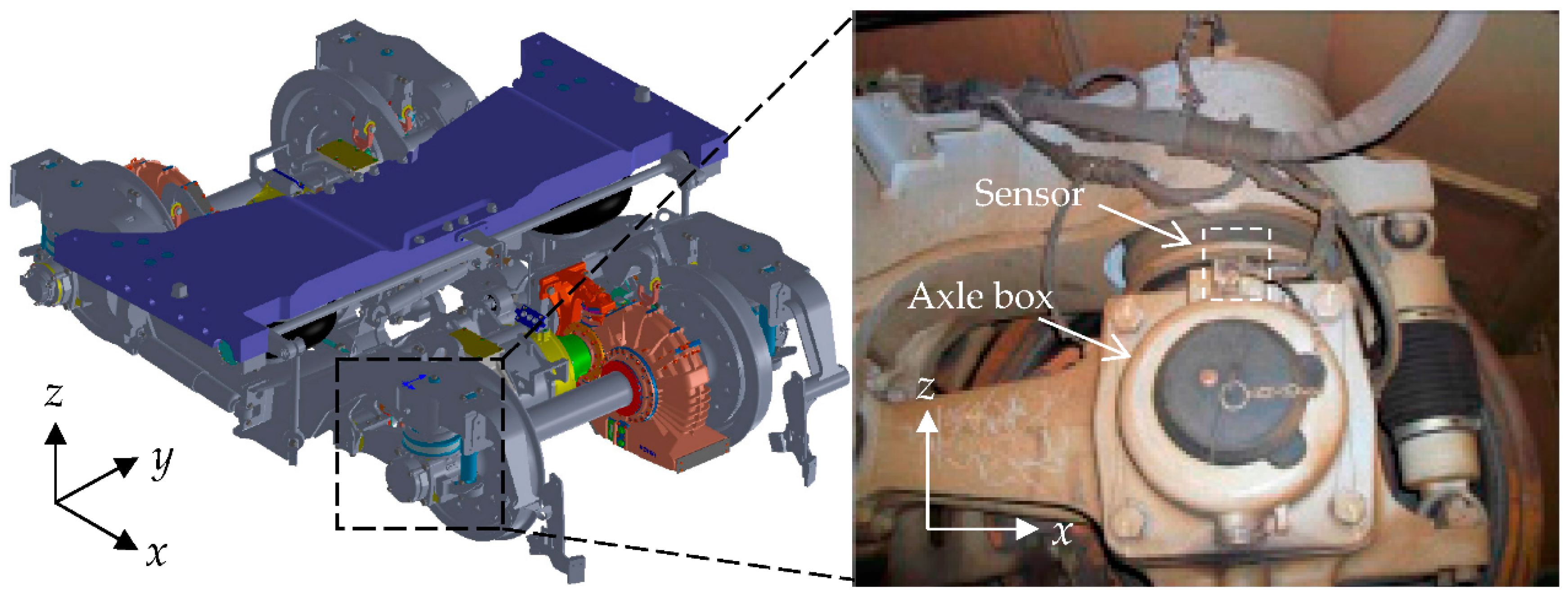
Figure 4.
Time-course response of measured ABA under 300 km/h. RW1 and RW2 are two examples of rail welds.
Figure 4.
Time-course response of measured ABA under 300 km/h. RW1 and RW2 are two examples of rail welds.
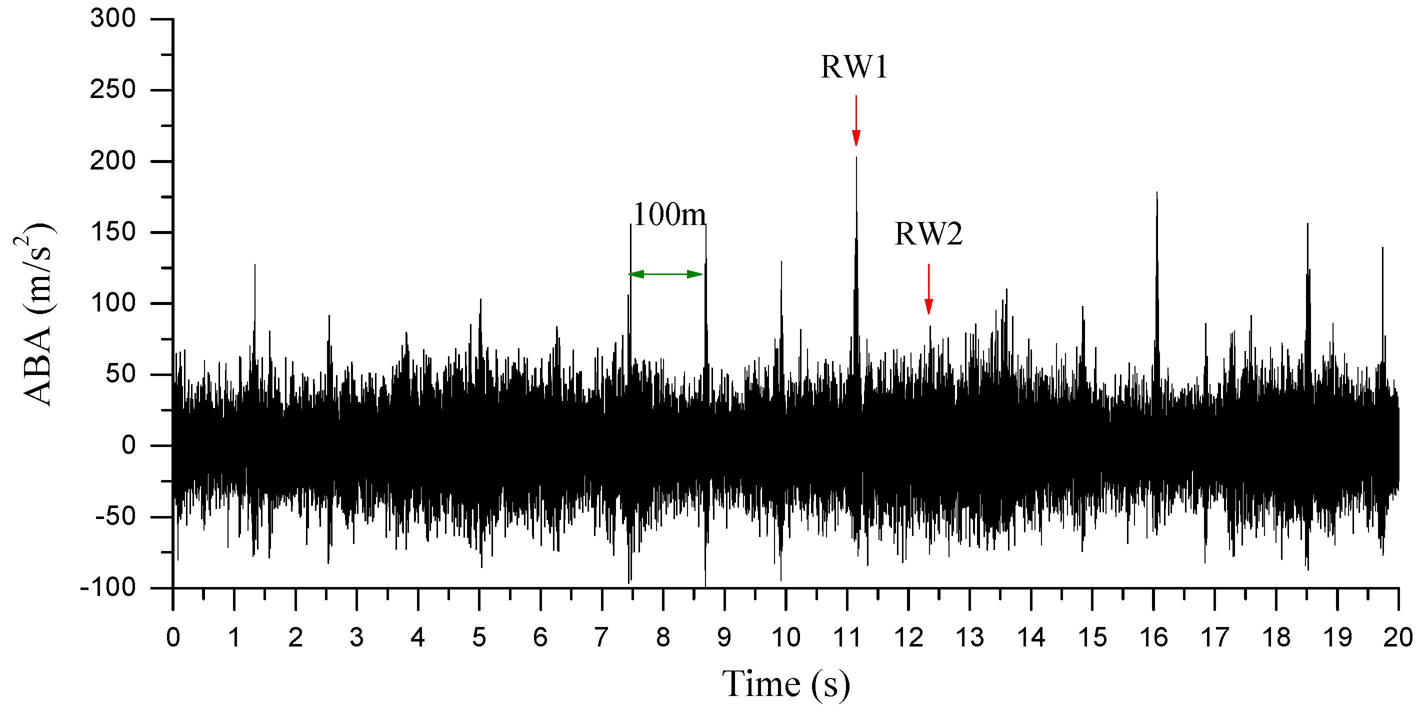
Figure 5.
The response of ABA in (a) time and (b) time–frequency domain when a vehicle passes the rail welds at a speed of 300 km/h on a certain high-speed line.
Figure 5.
The response of ABA in (a) time and (b) time–frequency domain when a vehicle passes the rail welds at a speed of 300 km/h on a certain high-speed line.

Figure 6.
Cumulative distribution function (CDF) of 17 measured ABAs induced by rail welds.

Figure 7.
3D wheel/rail rolling contact fine element model.
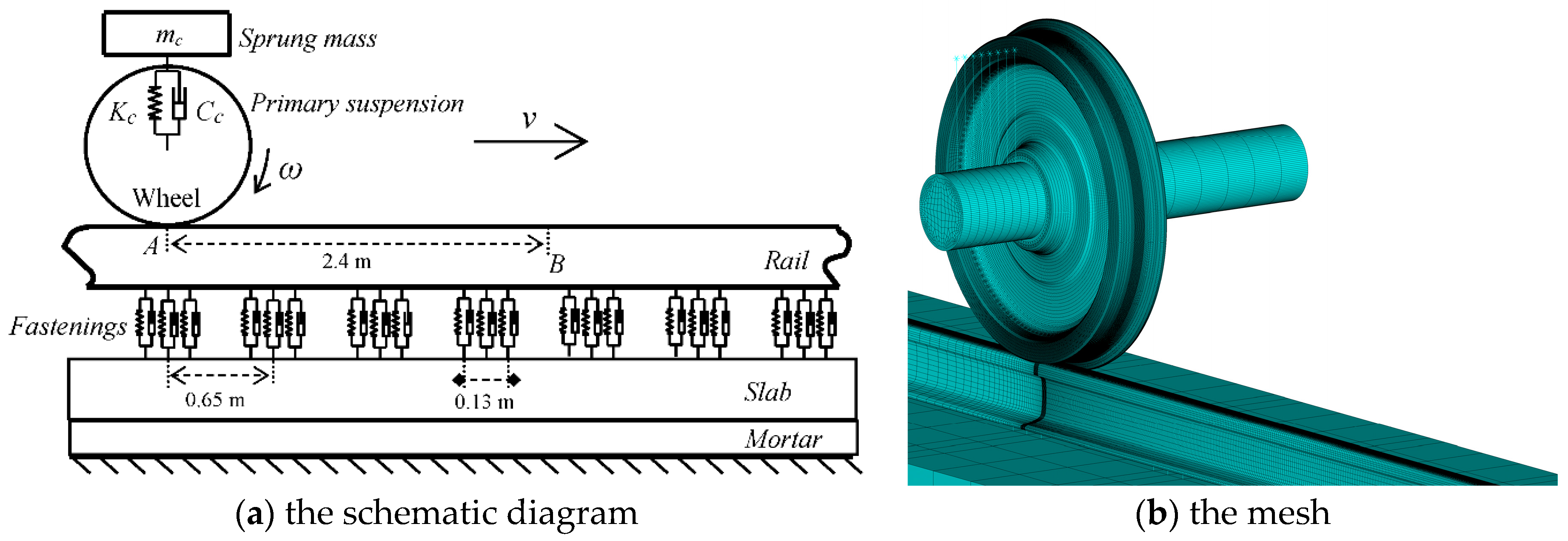
Figure 8.
Simulated rail weld geometry in (a) 2D and (b) 3D.

Figure 9.
Schematic diagram of the simulation process.
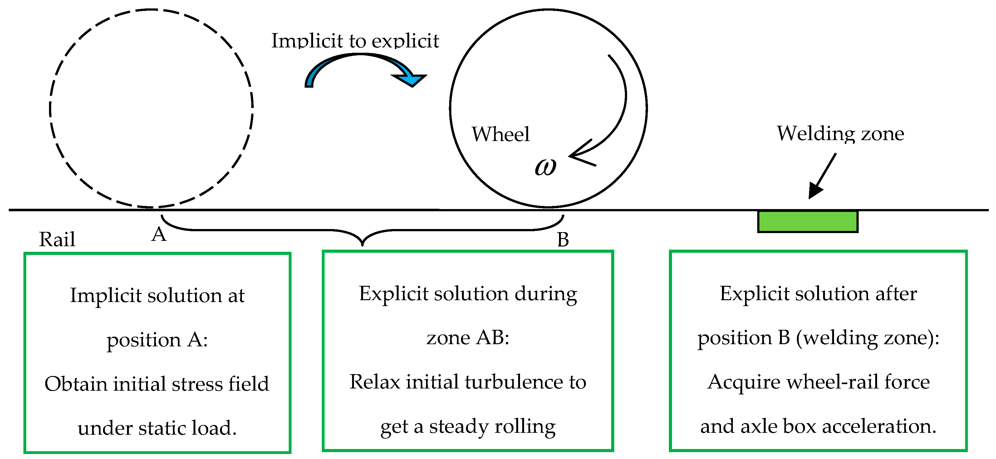
Figure 10.
The response of ABA under excitation of rail welds at different wavelengths in (a) time and (b) frequency domains.
Figure 10.
The response of ABA under excitation of rail welds at different wavelengths in (a) time and (b) frequency domains.
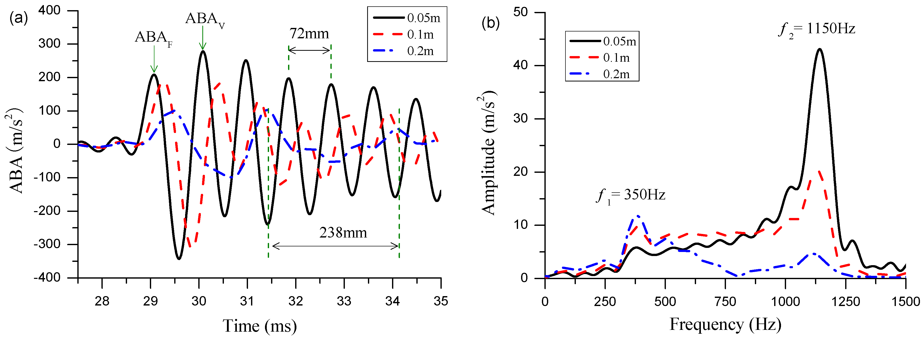
Figure 11.
The influence of wavelength on (a) ABA and (b) variation of amplitude at f1 and f2.

Figure 12.
The influence of wave depth on ABA in (a) frequency and (b) time domains.

Figure 13.
The response of wheel–track force under excitation of welds with different wavelengths.
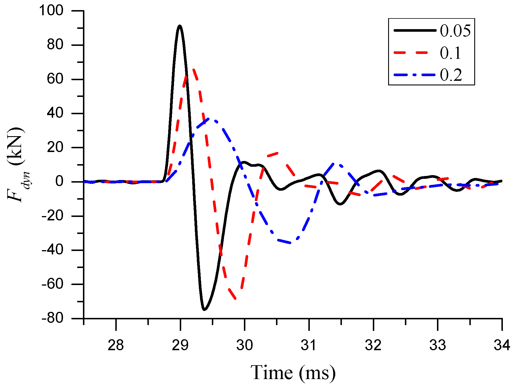
Figure 14.
The relationship between ABAF and Fdyn,max.

Figure 15.
Flowchart of an approach to estimate rail weld.

Figure 16.
Rail corrugation (a) and wheel flat (b).
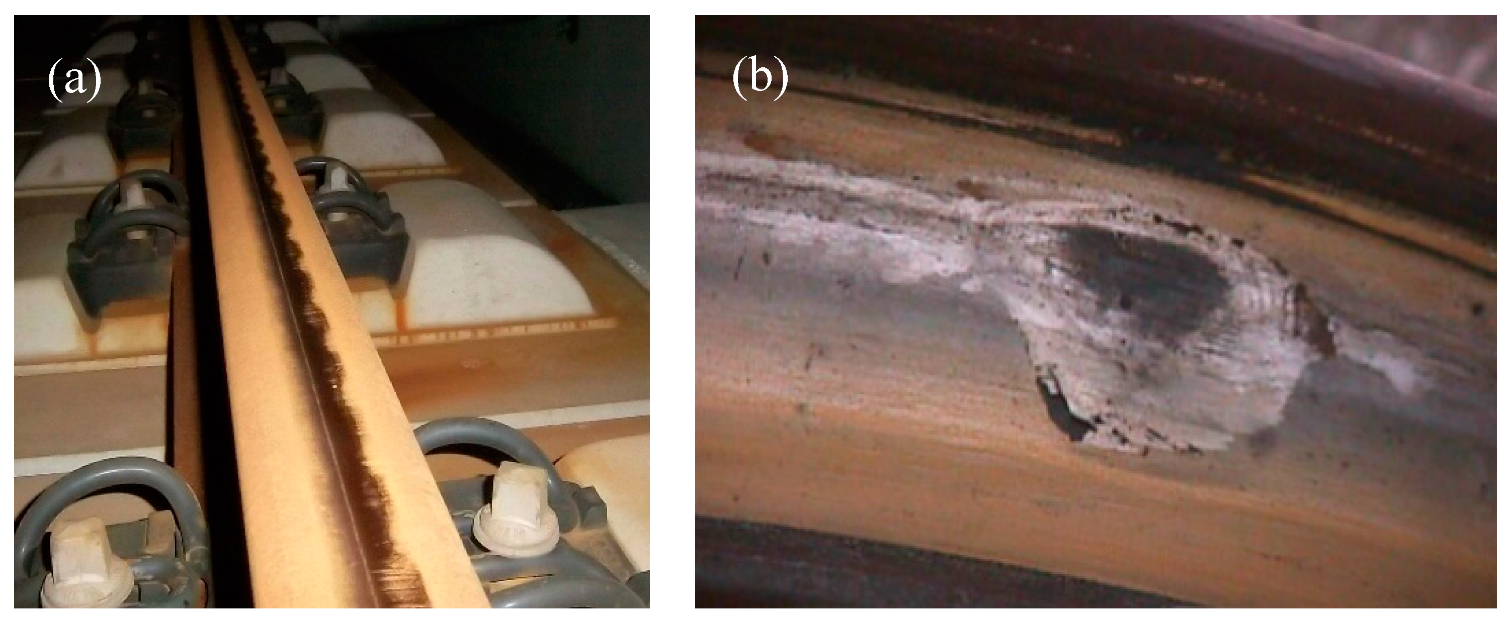
Figure 17.
Schematic diagrams of axle box acceleration induced by (a) rail corrugation and (b) wheel flat.
Figure 17.
Schematic diagrams of axle box acceleration induced by (a) rail corrugation and (b) wheel flat.

Table 1.
Values of the parameters involved in this work.
| Parameters | Values | |
|---|---|---|
| Lumped sprung mass | 7500 kg | |
| Stiffness of primary suspension | 880 kN/m | |
| Damping of primary suspension | 4 kNs/m | |
| Stiffness of fastenings | 22 MN/m | |
| Damping of fastenings | 200 kNs/m | |
| Wheel and rail material | Young’s modulus | 205.9 GPa |
| Poisson’s ratio | 0.3 | |
| Density | 7790 kg/m3 | |
| Material of pre-fabricated slabs | Young’s modulus | 34.5 GPa |
| Poisson’s ratio | 0.25 | |
| Density | 2400 kg/m3 | |
| Mortar material | Young’s modulus | 8 GPa |
| Poisson’s ratio | 0.2 | |
| Density | 1600 kg/m3 | |
© 2017 by the authors. Licensee MDPI, Basel, Switzerland. This article is an open access article distributed under the terms and conditions of the Creative Commons Attribution (CC BY) license (http://creativecommons.org/licenses/by/4.0/).
Share and Cite
MDPI and ACS Style
An, B.; Wang, P.; Xu, J.; Chen, R.; Cui, D. Observation and Simulation of Axle Box Acceleration in the Presence of Rail Weld in High-Speed Railway. Appl. Sci. 2017, 7, 1259. https://doi.org/10.3390/app7121259
AMA Style
An B, Wang P, Xu J, Chen R, Cui D. Observation and Simulation of Axle Box Acceleration in the Presence of Rail Weld in High-Speed Railway. Applied Sciences. 2017; 7(12):1259. https://doi.org/10.3390/app7121259
Chicago/Turabian StyleAn, Boyang, Ping Wang, Jingmang Xu, Rong Chen, and Dabin Cui. 2017. "Observation and Simulation of Axle Box Acceleration in the Presence of Rail Weld in High-Speed Railway" Applied Sciences 7, no. 12: 1259. https://doi.org/10.3390/app7121259
Note that from the first issue of 2016, this journal uses article numbers instead of page numbers. See further details here.