Article

Manufacturing Scheduling Using Colored Petri Nets and Reinforcement Learning

Alexander Technological Educational Institute of Thessaloniki, Department of Automation Engineering, P.O. Box 141, GR-57400 Thessaloniki, Greece
*
Author to whom correspondence should be addressed.
Appl. Sci. 2017, 7(2), 136; https://doi.org/10.3390/app7020136
Submission received: 23 December 2016 / Revised: 18 January 2017 / Accepted: 20 January 2017 / Published: 3 February 2017
(This article belongs to the Special Issue Modeling, Simulation, Operation and Control of Discrete Event Systems)

Abstract

:
Agent-based intelligent manufacturing control systems are capable to efficiently respond and adapt to environmental changes. Manufacturing system adaptation and evolution can be addressed with learning mechanisms that increase the intelligence of agents. In this paper a manufacturing scheduling method is presented based on Timed Colored Petri Nets (CTPNs) and reinforcement learning (RL). CTPNs model the manufacturing system and implement the scheduling. In the search for an optimal solution a scheduling agent uses RL and in particular the Q-learning algorithm. A warehouse order-picking scheduling is presented as a case study to illustrate the method. The proposed scheduling method is compared to existing methods. Simulation and state space results are used to evaluate performance and identify system properties.

1. Introduction

Flexibility, cost reduction, production efficiency, improved inventory control, and ability to respond to fluctuations in demand are among the drivers for innovative automated solutions to all members of a supply chain. Manufacturing scheduling is the optimization process of assigning a limited number of resources within a temporal horizon to a set of manufacturing processes of a plan subject to a set of constraints [1]. Computation time to obtain a global optimum increases exponentially with problem size, as such scheduling is generally considered NP-hard (non-polynomial hard) [1,2,3], whereas integrated process planning, scheduling and control, and dynamic response to emergence increase the complexity of manufacturing scheduling. New generation real-time control systems allow optimal performance under different conditions for flexible, autonomous, and adaptive manufacturing systems, generally called intelligent manufacturing systems, such as multi-agent systems (MAS) and Holonic Manufacturing Systems (HMS) [2]. The application of agent technologies in manufacturing supports distributed control and execution, and provides robustness, reconfigurability, and re-usability. The new generation of manufacturing control systems may exhibit self-organization and emergent behavior in order to respond to environmental changes [2]. Learning is a key method used for this purpose in agent-based manufacturing systems [4].
Various definitions for the term “agent” exist. In Wooldridge [5], “an agent is a computer system that is situated in some environment and that is capable of autonomous action in this environment in order to meet its design objectives”. The most important properties of an agent for manufacturing systems are autonomy, intelligence, adaptation, and co-operation [2]. An agent can increase its intelligence through learning. Reinforcement learning (RL) is a procedure for an agent to learn to act optimally to achieve its goals through interaction with its environment. For scheduling, the learning task is to produce a scheduling action that will lead to minimize (or maximize) the related performance measure. A widely used RL algorithm is Q-learning [6,7].
Petri Nets (PNs) and Colored Petri Nets (CPNs) are a discrete-event graphical and mathematical modeling tool applicable to systems characterized as being concurrent, asynchronous, distributed, parallel, nondeterministic, and/or stochastic [8,9]. As such, they have been used extensively for modeling, scheduling, and control of Flexible Manufacturing Systems (FMS). Their main features for this purpose can be described as a powerful modeling ability to describe concurrent, synchronous, conflict, and casual behavior; logic properties (such as boundedness, liveness) and control logic code generated directly from PNs [10]; and the performance evaluation of the system [10,11], including the ability to represent many states concisely, as well as to model precedence relations, deadlocks, conflicts, and resource constraints [12,13]. CPNs can represent parts with attributes as well as temporal activities (Timed Colored Petri Nets, CTPNs). CPN is a discrete-event modeling tool combining PNs with the functional programming language Standard ML [14]. As a graphical-oriented high-level language, it is used for the modeling and validation of systems in which concurrency, communication, and synchronization play a major role. This is why it finds many applications in the area of distributed artificial intelligence (AI) where agents come from.
Combinations of PNs- and AI-search based techniques have found applications to manufacturing scheduling, where PNs model the system and a heuristics based search through the reachability graph finds an optimal or near-optimal solution. However, these methods are not as efficient for large, complex manufacturing systems in changing environments. Moreover, CPNs are more suitable for modeling complex manufacturing systems. In this paper a CTPN-based manufacturing scheduling method is presented. CTPNs model an agent-based system and the Q-learning RL algorithm is used by the scheduling agent as a guide to obtain an optimal solution. In order to evaluate the proposed method, it is compared to existing scheduling methods applied to known job shop benchmark examples. A warehouse order-picking scheduling is used as a case study to illustrate the applicability of the method.
The rest of the paper is organized as follows. A literature review is given in Section 2. The scheduling method is presented in Section 3. It is illustrated with a case study in Section 4. In Section 5 the performance evaluation and verification of PN-related system properties are given using simulation and state space report results. Conclusions are presented in Section 6.

2. Literature Review

2.1. PNs and CPNs Combined with AI Techniques for Manufacturing Scheduling

CPNs are a discrete-event graphical language used to construct models of distributed, concurrent systems, and discover their properties. PN and CPN models consist of places, transitions, and arcs (joining places and transitions). Transitions and arcs represent events that could cause state changes and their interactions, respectively. Tokens reside in PN places and their number controls the firing of transitions (i.e., system changes). The distribution of tokens on the places, i.e., the marking, represents the state of the system. However, for large complex systems, the size of the PN system model becomes too large to be tractable. CPNs overcome this limitation by the use of color tokens, i.e., tokens with attached data types, and by the use of hierarchical CPNs. Hierarchical CPNs are used to model complex systems by structurally decomposing system modules to submodules. CPN simulation modeling enables investigation of the system behavior by studying the various ‘what-if’ system scenarios. Time integration (deterministic or stochastic time) in the system model allows the investigation of simulation-based performance measures, such as delays and throughput, as well as modeling of real-time systems. While the graphical aspect of CPNs allows visualization of the modeled system, the mathematical aspect of CPNs allows the set-up of mathematical models governing the behavior of the systems [9] and verification of system properties by means of state space analysis methods. State space analysis identifies all possible reachable states and state changes of a system model, and visualizes the results as a directed graph where nodes represent system states, and arcs represent occurring events. It allows verification of behavioral properties of the system, such as boundedness, home properties, liveness, and fairness. State space exploration allows the automatic detection of all events in a system state, analysis of the cause–effect event relationship, as well as control of system behavior [15].
CPNs provide a modeling formalism that can support the decision-making process of logistics systems, i.e., systems with stochastic, asynchronous, and dynamic behavior [15,16]. Manufacturing scheduling is an optimization process, considered as NP-hard problem. Reviews of PN/CPN applications in modeling of FMS and production scheduling have been presented (e.g., [13,17]). Scheduling and control schemes based on combinations of AI techniques and PNs/CPNs aim to explore the advantages of both techniques. AI techniques used for PN based manufacturing scheduling include heuristic rule based methods, heuristic search algorithm methods, mathematical programming methods, expert systems and knowledge-based systems, and distributed AI methods based on MAS and HMS.
In heuristic rule-based methods, PNs model the manufacturing system, whereas heuristic rules aim to resolve the scheduling conflicts. However, they were developed for specific classes of problems (e.g., [18,19]). Exploration of state space methods, i.e., expansion of the reachability graph, in order to find an optimal solution is difficult due to the state space explosion problem even for small systems. Modeling approaches that have been introduced to handle the state space explosion include stochastic well-formed colored nets (SWNs) [20] and Markovian Agents [21]. SWNs were introduced together with a symbolic reachability graph construction algorithm that allows reduction of the Markov chain obtained by CPNs or other classical High-level PNs by exploiting the system symmetries. In Castiglione et al. [21] an analytic modeling technique based on the use of Markovian Agents and Mean Field Analysis has been proposed that allows the effective modeling of concurrent Big Data applications. In heuristic search algorithm methods, PNs model the system and a search algorithm based on a heuristic function is used to expand a portion of the reachability graph, containing the most promising nodes that leads to an optimal scheduling solution [3,22,23,24,25,26,27,28,29,30,31,32,33,34,35,36]. The heuristic function must be admissible in order to obtain the optimal solution. In Lee and DiCesare [3] a heuristic search algorithm based on the A* algorithm, a branch and bound type algorithm, was introduced to limit the search in the PN reachability graph in order to find the optimal solution for FMS scheduling problems. Modified and improved versions of the A* based heuristic search method have been presented in the literature [25,26,27,28,29,30,31,32,33,34,35,36]. In order to reduce the search time, non-admissible heuristic functions were proposed in [31,32]. A heuristic search method for FMS scheduling based on combination of admissible and non-admissible heuristic functions in the A* algorithm was presented in [33].
In the area of agent-based systems and HMS both PNs and CPNs have found applications. A predicate/transition net model for a robotic MAS planning has been presented in Murata et al. [37]. A formal methodology for the modeling and validation of the ADACOR-holonic architecture has been proposed in Leitao et al. [38], aiming to improve the performance of control systems in industrial scenarios. A framework to model and control HMS has been suggested in Hsieh [39] based on fusion of CPNs and multi-agent system theory. The problem of managing and controlling automatic guided vehicles (AGVs) in manufacturing shop floor systems using an agent-based PN model has been addressed in Giglio and Paolucci [40]. PN modeling of FMS with random recipes and control with an agent-based architecture has been proposed in Castelnuovo [41]. The model was implemented in the agent platform JADE. A CPN model to represent relative dynamic factors in agent-based scheduling and planning systems that can analyze future states of a system has been proposed in Bai et al. [42]. A PN model to represent the interaction protocols between order and resource agents in a holonic manufacturing execution system, and a game theoretic approach to analyze the possible outcomes of the negotiation process have been presented in [43]. A CTPN-based method was presented in Drakaki and Tzionas [44] to model an agent-based warehouse control system in order to evaluate system properties and performance. The method was applied to a dynamic resource allocation of an order-picking process.
A new class of PNs, object-oriented knowledge-based PNs, incorporating knowledge-based expert systems and fuzzy logic into ordinary PNs, was introduced and used for integration of design and assembly planning processes in manufacturing in Huang [45]. A fuzzy PN model to represent the fuzzy production rule of a rule-based system has been proposed in Chen et al. [46]. Applications of PNs in AI have been explored in Joseph [47] and an application was shown to a rule-based production system. A knowledge PN-based AI protocol that integrated knowledge based expert system and fuzzy logic with ordinary PNs was defined and used for intelligent integration of product design [48]. In Zha et al. [49] a fuzzy expert PN method was presented that integrated knowledge-based systems, fuzzy logic, and artificial neural networks. A generic expert PN model of a single neuron was presented using the method. Knowledge Attribute PNs were introduced in Jávor [50] enabling mobile knowledge bases attached to tokens. By using the combination of PNs and AI, the method aimed to enhance the effectiveness of modeling and simulation in applications including FMS.

2.2. Reinforcement Learning

Intelligent agents are composed of a perception mechanism, a cognition system, and an action module. They receive messages from the environment using the perception mechanism, evaluate the messages using the cognition module, and produce actions by the action module [5,51,52]. Learning and evolving are key mechanisms in intelligent agents. RL is a widely used method for this purpose. RL is the procedure by which an agent learns from interaction with its environment to achieve a goal, in general to obtain its own optimal control policy. A complete specification of an environment defines a task. At each time step, the agent receives some representation of the environment’s state, from the set of possible states, and on that basis selects an action from the set of available actions. One time step later, in part as a consequence of its action, the agent receives a numerical reward, and finds itself in a new state. At each time step, the agent implements a mapping, called a policy, from states to probabilities of selecting each possible action. RL methods specify how the agent changes its policy as a result of its experience. The agent’s goal is to maximize the total reward it receives over the long run [6].
RL problems can be solved using dynamic programming (DP) algorithms, although the time required for large problems may make their solution infeasible. Q-learning is a model-free RL algorithm that approximates DP [7]. The Q-learning algorithm estimates the value functions, Q(s,a), of state-action pairs. Q(s,a) is a discounted sum of future rewards. Once these values have been learned, the optimal policy, π*(s), from any state is the one with the highest Q-value. This algorithm converges to the optimal value functions, Q*(s,a), representing the optimal policy, for RL tasks that satisfy the Markov property, called Markov Decision Processes (MDPs). For Markovian environments the current state summarizes the history of past states, thus all the information an agent needs to take an action and make a transition from its current state to a next state is stored in its current state. If an agent learns the Q-values, then it can make optimal decisions at each state.
RL has been applied to manufacturing scheduling [51,53,54,55,56,57,58,59]. A single machine agent used Q-learning to determine if it could learn commonly accepted dispatching rules for three example cases in which the best dispatching rules had been previously defined in Wang and Usher [53]. Agents were trained to an RL algorithm, called Q-III, used for dynamic job shop scheduling to select the most appropriate priority rule according to the shop conditions in real time in Aydin and Oztemel [51]. The temporal difference algorithm TD(λ), an RL algorithm, has been applied to job shop scheduling involving the scheduling of the various tasks that had to be performed to install and test the payloads placed in the cargo bay of the NASA space shuttle for each mission [54]. The objective was to schedule a set of tasks without violating any resource constraints while minimizing the total duration. An RL algorithm, called SMART, was developed and applied to the case of optimal preventative maintenance in a production inventory system [55,56]. SMART was applied to the problem of optimizing a three- and four-machine transfer line, respectively, producing a single product type [57,58]. The system goal was to maximize the throughput of the transfer line while minimizing work-in-process and failures. Dynamic control policies were obtained for a stochastic lot production scheduling problem using an RL-based approach implemented by a multi-agent control architecture [59]. A Neural Network-based approach was used to approximate the reinforcement value function. In Gabel and Riedmiller [60] a production scheduling method was presented where the scheduling problems were modeled as multi-agent RL problems. Resource agents made independent job dispatching decisions and improved their decisions by employing RL. The RL algorithm was based on neural network-based value function approximation and an optimistic inter-agent coordination scheme. In Csáji et al. [61] an agent-based market-based production control system was presented with learning and cooperative agents. A triple level learning mechanism was proposed, including simulated annealing, RL, and an artificial neural network.

3. Methodology

The method is based on hierarchical CTPNs. Scheduling is done by a single agent. The agent interacts with its environment in order to do the scheduling. At each step, t, the agent observes the state st, s ∈ S, of the environment, follows a policy πt, and selects an action at ∈ A(s). As a result of its action, it receives an immediate reward rt ∈ R, and the state of the environment changes to st+1 ∈ S [6]. The policy, πt, is a mapping from states to action probabilities: πt(s,a) = probability that at = a when st = s. The agent’s goal is to obtain an optimal policy, π*.
The value of a state, Vπ(s), under a policy π, is the expected reward the agent receives, when it starts from that state, s. The action-value (Q-value), Q(s,a), is the expected reward the agent receives under policy π, when it chooses an action a at state s, The agent follows π thereafter. The optimal action-values Q*(s,a) are obtained when the agent follows an optimal policy, π*. There is a unique solution for the value of a state under an optimal policy, V*(s), V*(s) = maxaQ*(s,a). If a* is an action that maximizes Q*(s,a), then π*(s) ≡ a* = arg(maxaQ*(s,a)) [7].
The top CTPN model page includes the submodels of the scheduling agent and the simulation environment. The simulation environment submodel consists of the set of jobs, job data and job characteristics and set of machines. The scheduling agent submodel consists of a heuristics rule base submodel and an intelligent part submodel. The heuristics rule base submodel may be used depending on the scheduling problem.
The intelligent part submodel consists of a perception module, a Q-learning module and an action module. The perception module perceives the current state of the environment. The information about the current state is received by the Q-learning module. The Q-learning submodel selects a policy action, a, for the current state, s, from a set of available policy actions. As a result of the agent’s action, the environment arrives at a new state, s′. The agent perceives the new state and receives an immediate reward, r, by the perception submodel. In each scheduling cycle the Q-learning is implemented by the agent to guide it to the optimal scheduling decision. The implementation is based on the following steps [7]:
(1)
The agent perceives the current state, s and selects an action a. Based on its action it receives an immediate reward, r and arrives at the next state, s′.
(2)
Q(s,a) values are updated as
Q ( s , a ) : = Q ( s , a ) + α ( r + γ   max b Q ( s , b ) Q ( s , a ) ) .
(3)
Go to (1) until s is a terminal state,
where α is the learning rate and γ, 0 ≤ γ < 1, is the discount factor. Steps (1)–(3) are steps of one episode which ends when a terminal state is reached. A number of episodes take place. The Q(s,a) values represent the long term reward. The learning rate determines the influence of the old Q(s,a) values on the new ones. The discount factor determines whether the agent takes into account immediate rewards more strongly than rewards received previously. The agent has the option of following an ε-greedy method in the training period, i.e., to randomly select an action for a percentage of time defined by ε.
The agent tries to maximize its long-term reward, i.e., the Q(s,a) values for each state action pair, thus the immediate reward guides the agent as to what action to take next. The minimal makespan is the scheduling objective considered as the optimality criterion in this paper. Makespan, i.e., C max max j J { C j } , where J = {1, …, n} is the set of n jobs, and C j is the completion time of job j, is a widely used manufacturing scheduling objective.
The state of the system is the criterion taken into account by the agent in order to decide its next policy action. Available policies are modeled as CTPN models. The calculated makespan extracted from simulation is used as the state determination criterion. A number of policy states are generated, whereas policy actions implement related scheduling rules, such as dispatching rules (e.g., Shortest Processing Time (SPT), Longest Processing Time (LPT), First-in, First-Out (FIFO)), for job shop scheduling). Each policy action is a generation of a complete schedule by the agent. Each generated schedule is a possible solution. It corresponds to a path from the initial marking to a final marking in the CPN reachability graph, as well as a node in the calculated state space. During the training period, the agent is trained using the Q-learning for 1000 cycles (episodes). Each cycle (episode) is associated with a model index ranging from 1 to 1000. The value of each index along with the associated starting and end times of jobs, the makespan, and the environmental state are stored in a list (a knowledge base). During the 1000 cycles the Q-learning converges to a predefined (dummy) terminal state corresponding to the optimal makespan solution a number of times. At the end of 1000 cycles, the indices and the corresponding makespan values of the dummy terminal state are retrieved. Then, the lowest makespan value is chosen and the scheduling that led to the minimal makespan is retrieved from the knowledge base.

4. The Case Study

4.1. The Order-Picking Process

A high-volume small parts spread buffer order-picking scheduling system is presented as a case study to illustrate the method. In this class of picker-to-goods order picking systems, item retrieval is decoupled from order assembly by a pick-to-buffer (P2B) technology [62]. In a P2B system items retrieved from pick locations are placed into a pick buffer. Items are deposited automatically into an order container placed on a conveyor when all items of an order have been picked. The physical layout of the order-picking system consists of four pick zones with a common conveyor. Robotic order-picking is considered. Each pick zone is assigned to a gantry robot. A pick zone consists of 30 product totes with each tote having 40 compartments. A compartment can accommodate 20 product units of one Stock Keeping Unit (SKU) type. The order-picking process is a sequential zone picking with batching. The order containers of each batch pass sequentially from one pick zone to the next one and all items to be picked in each zone are picked in one pass. Gantry robots can pick one product item at a time and deposit it in the nearest buffer. Customer orders are organized in five batches of 28 order containers each. Each order container contains a single customer’s order and can have multiple line items. One SKU type is collected in every order-picking process. A line item is a single unit of product. The conveyor speed is constant. Randomized storage is assumed. Figure 1 shows the layout of a pick zone (after [63]).

4.2. The Order-Picking Scheduling

The scheduling problem consists of two parts, i.e., order batching including routing, and sequencing. A system assumption is that the SKUs are high demand products distributed in each zone, each one located in two pick locations in each zone.

4.2.1. Order Batching

Order batching is calculated based on the following two-step heuristic [44]. The agent’s goal, in this stage is a balanced workload among robots.
Step 1: The first incoming order to the system goes to the first batch. The second order goes to the second batch, until each batch has one order. The next order goes to the batch with the least workload. All the remaining orders are assigned following this rule.
Step 2: The average workload per pick zone is calculated. Next, for each batch, orders are assigned to pick zones 1 through 4, so that the workload per pick zone does not exceed the average workload, starting from pick zone 1.

4.2.2. Order Sequencing

Order-picking sequencing involves the generation of the order-picking sequence for each robot by the agent. In this scheduling step, the agent employs the Q-learning in order to make the optimal decision. The agent’s goal that guides it to the optimal scheduling decision is to achieve the minimal total robot travel time for each batch of orders.
Picker travel time is an important parameter in the design of order picking systems. For the system under consideration robot travel time impacts the learning capability developed by the agent, i.e., the optimal order sequencing. It is a parameter affecting the environment’s state and immediate reward calculation, thus the Q-values. Robot movement is characterized by the Chebyshev metric. A gantry robot is characterized by linear movement, thus its position is specified using the Cartesian coordinate system. Independent motors permit simultaneous movement in both horizontal and vertical planes. If the robot moves between two points in the pick area (xy plane), with coordinates (x1, y1) and (x2, y2), according to the Chebyshev metric it travels a distance equal to max(|x2x1|, |y2y1|). Thus, the travel time between two points depends on the maximum of the horizontal and vertical movement times [63]. The robot pick travel time for the P2B system consists of the time it takes to move from a pick location to the closest empty buffer (loaded travel movement) and the time it takes to move from the buffer to the next pick location (empty travel movement). The parameters used in the system simulation for robot travel time calculation are: horizontal movement speed = 1.5 m/s, vertical movement speed = 0.4 m/s, length of a zone = 45 m, height of a zone = 2.4 m.
The Q-learning is employed by the agent for 1000 cycles in order to do the order sequencing for the current batch of orders. In each cycle the agent produces an order sequencing solution implemented by the CTPN system model. In each cycle, since each line item is located in two pick locations, the agent chooses randomly between the two possible locations and makes a list of the pick locations for each robot. Each agent policy action is the generation of the ordered list/sequence of the pick locations for each robot in the current batch by the agent. The agent can take one of the following two available policy actions in order to produce the order sequencing in each state:
(1)
use the X-coordinate based heuristic [63]. The sequencing of orders in each zone is done based on the increasing order of the X-coordinates of the SKU type locations, assuming that the length of each zone is much longer than its width.
(2)
Choose randomly the pick locations in each zone.
The state of the system is the criterion taken into account by the agent in order to decide its next action. For the order-picking scheduling case study, the total travel time of all robots for the current batch of orders, ttot, is the state determination criterion. It is calculated from the CTPN model simulation in each scheduling cycle. The scheduling policy includes 10 states, and two dummy states, shown in Table 1. The Q-values for all states were initialized to a value of zero, since no prior knowledge is known for any state. Robot travel times are calculated using the pick location information and the Chebyshev metric. The average total travel time used by the agent in order to perceive the current state is calculated from the average total travel time value, ttot,aver, calculated from 1000 replications of total travel time values of random lists of pick locations (pick tote and pick compartment locations) corresponding to the total line item number of the current batch of orders. The order sequencing for the calculation of average total travel time is done using the X-coordinate based heuristic. More specifically, it is assumed that the pick locations are not close to each other, thus since the length of the zone is much greater than the width, the horizontal movement times are longer than the vertical movement times. Therefore order sequencing is done based on the increasing order of the X-coordinates of the SKU type locations. The dummy terminal state corresponds to an optimal or near optimal solution.
Each time the agent takes an action, it receives an immediate reward (or a penalty), r, as a result of its action, and the Q-values are updated according to Equation (1). The immediate rewards should reflect the scheduling optimality criterion, i.e., the long term goal of the agent when it decides its next action. The immediate reward values, shown in Table 2, are related to the total travel time of all robots, ttot, for the current batch of orders, range from −4.0 to 4.5, and were chosen by trial and error.
The learning rate, α, and the discount factor, γ, are taken equal to 0.1 and 0.9 accordingly [6,53]. The agent can follow an ε-greedy method, with ε = 0.2, i.e., 20% of the time it randomly selects an action.
After the completion of the 1000 cycle period the agent selects the scheduling that minimizes the total travel time of all robots for the current batch of orders. In particular, in each scheduling cycle, the agent stores in a knowledge base a list the cycle index and the corresponding order sequencing. A separate list holds the cycle index and the corresponding total travel time of all robots. After the end of the scheduling cycle period the agent retrieves the minimal total travel time of all robots, and the associated cycle index. Finally, using the cycle index it retrieves the corresponding order sequencing.

4.3. The Implemented CTPN System Model

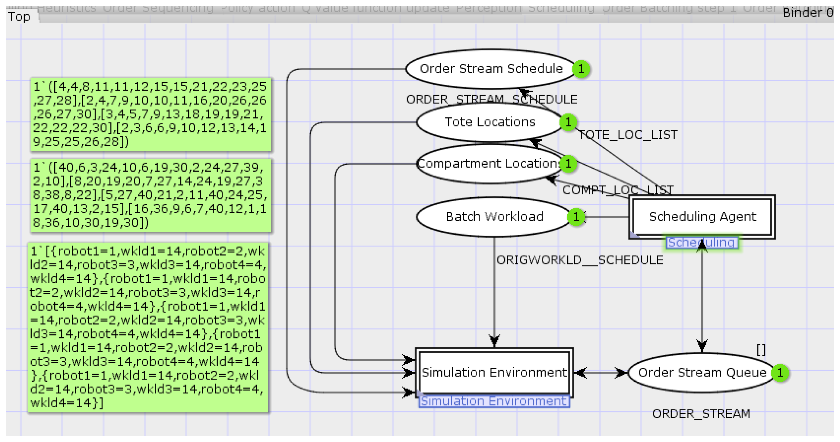
The hierarchical CTPN system model has been implemented using CPN Tools [64]. The top page of the implemented CTPN model shown in Figure 2 includes the Scheduling Agent and the Simulation Environment submodels as substitution transitions. Basic color set declarations of the CTPN model are shown in Table 3.
A substitution transition Order Arrivals in the simulation environment submodel generates the orders. A total of 140 orders are generated in discrete time steps. The order inter-arrival times are exponentially distributed with a mean inter-arrival time of 100 time units. The order color token is a record with fields: orderno (the order number), itemno (the number of line items), and AT (arrival time). The order size follows the binomial distribution function, with a mean of one to four line items. The list of orders, a token of color set ORDER_STREAM, is placed in place Order Stream Queue (place P1 in the top model page).
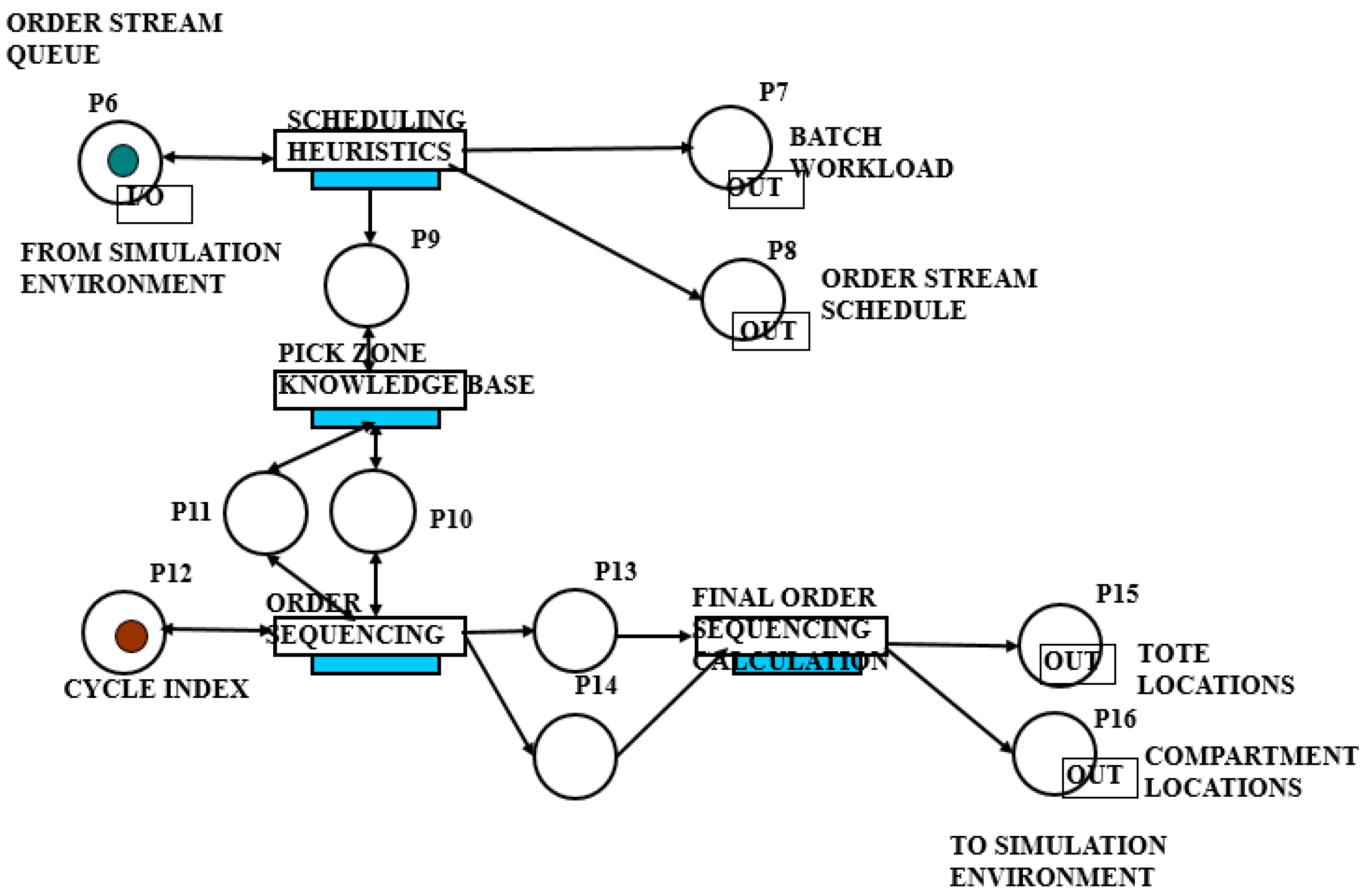
The Scheduling Agent submodel is shown in Figure 3. When the Scheduling Heuristics substitution transition receives the list of orders in place P6, it implements the order batching heuristic. The Scheduling Heuristics substitution transition includes the Create Batch Workload substitution transition and the Batch Routing substitution transition in order to implement the order batching heuristic. The Create Batch Workload substitution transition generates a list of five batches, a token of color set BATCH_LIST. BATCH_LIST, is a list of color set BATCH_INFO, a record with fields: batch_ord (the number of the batch of orders), batch_wkld (the list of orders included in the current batch), and batch_itm_cnt (the total number of line items included in the current batch). The Batch Routing substitution transition generates the routing for the batches of orders. The Scheduling Heuristics output tokens are placed in places P7, Batch Workload and P8, Order Stream Schedule (places P2 and P3 in the top model page, respectively). Place Batch Workload holds the workload per pick zone for all five batches. Place Order Stream Schedule holds the schedule for all five batches. Each customer order in the Order Stream Schedule output token is represented by a record with fields orderid (the order entry number, prodno (SKU type), lnitmno (number of line items), and pickzono (pick zone number).
The Scheduling Heuristics output token for a batch of orders is placed in place P9. The pick zone knowledge base substitution transition is then enabled. Its output tokens, held in places P10 and P11, are the possible pick locations (tote number and compartment number) for the line items to be picked from each zone. Pick locations are generated using the discrete uniform distribution. discrete(1,30) generates the available pick zone tote locations and discrete(1,40) generates the available compartment locations for each line item. Line items can be retrieved from two possible locations in each zone.
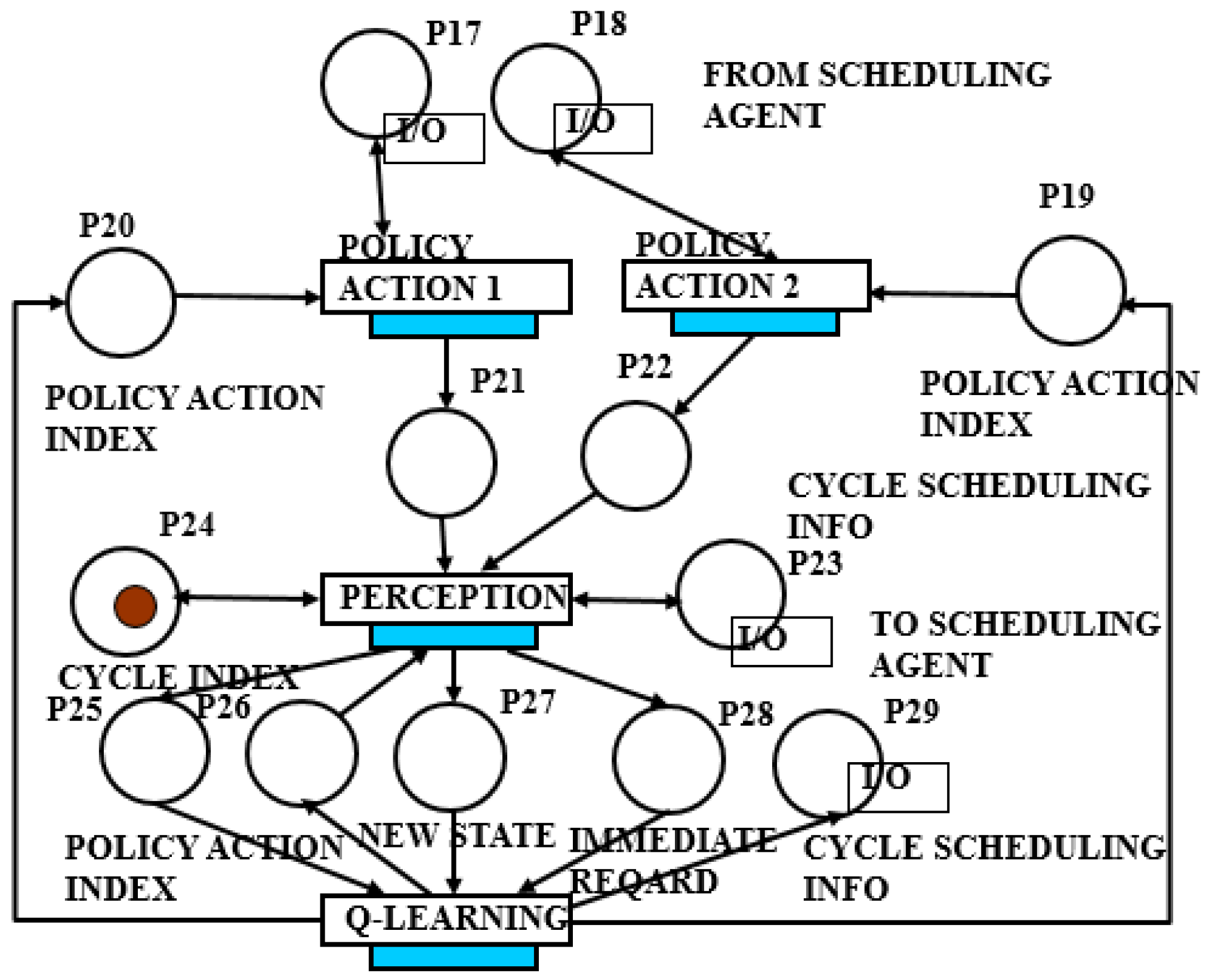
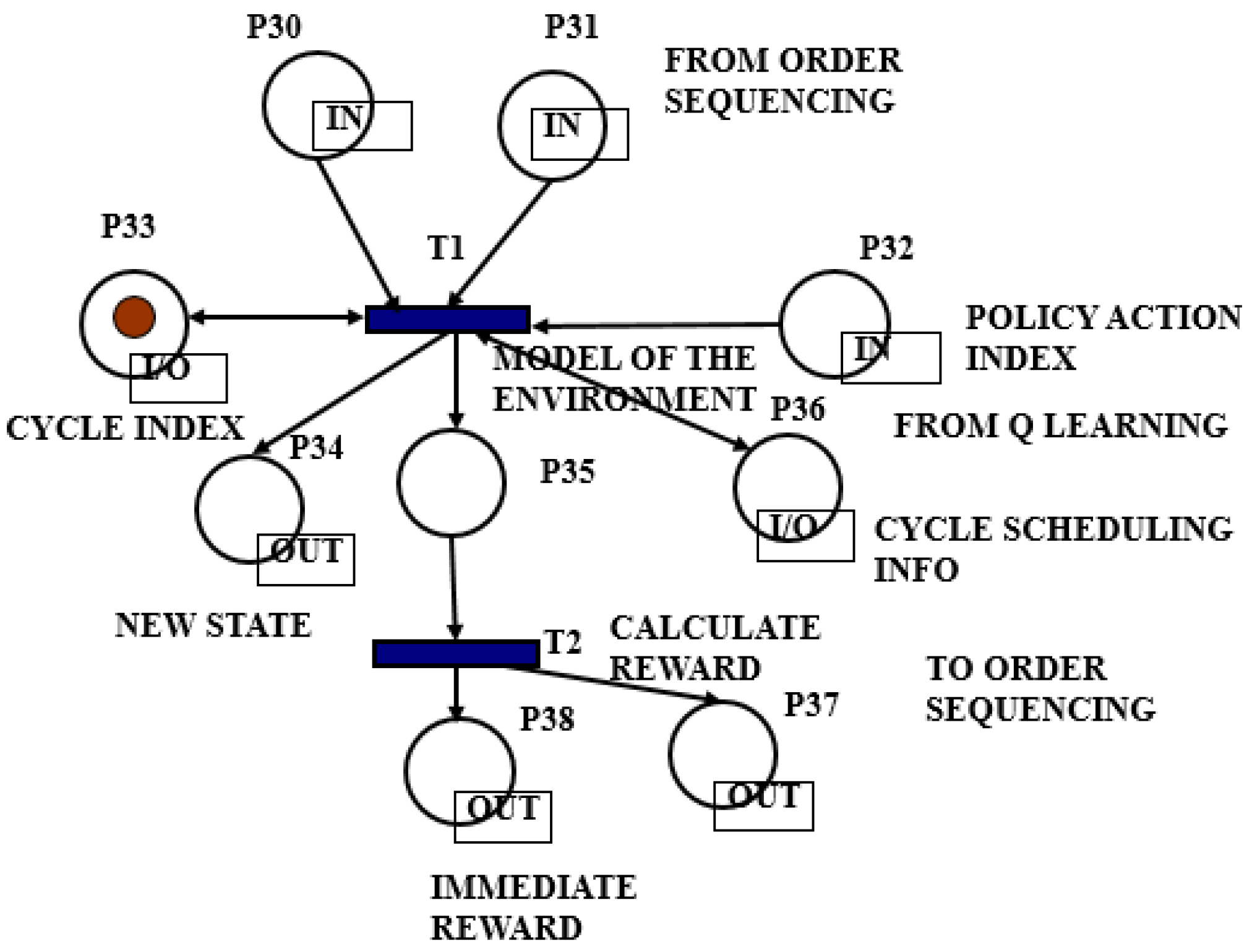
The Order Sequencing substitution transition is then enabled. The scheduling agent starts the scheduling cycles (a total of 1000) for the current batch of orders. Place P12 generates the Scheduling cycle index, a token of color set INT, ranging from 1 to 1000. The Order Sequencing substitution transition is shown in Figure 4. The Policy action 1 and Policy action 2 substitution transitions output pick locations to places P21 and P22 respectively. Pick locations are chosen for each line item from the corresponding input lists, held in places P17 and P18, representing available pick zone tote and compartment locations. Either Policy action 1 or Policy action 2 substitution transition is enabled, depending on the value of the policy action index token (places P19 and P20). The policy action index takes the values 1 or 2, depending on the action that the scheduling agent decides to take in each state based on the policy table (Table 1). The Perception substitution transition, shown in Figure 5, receives the calculated robot travel times in each zone, a result of the chosen policy action by the agent. Then, the Model of the Environment transition, T1, fires and outputs the new state color token, i.e., the new state, of color set INT, calculated based on the policy table state definitions (Table 1). Next the Calculate Reward transition, T2, fires and calculates the immediate reward, a token of color set REAL, based on the immediate reward value definitions (Table 2). Perception outputs to place P23 of the Order Sequencing substitution transition a cycle scheduling information token, a list with elements the cycle index and the order sequencing for each pick zone. The immediate reward and new state Perception output tokens are input tokens (in P27 and P28 places, respectively) to the Q-Learning substitution transition.
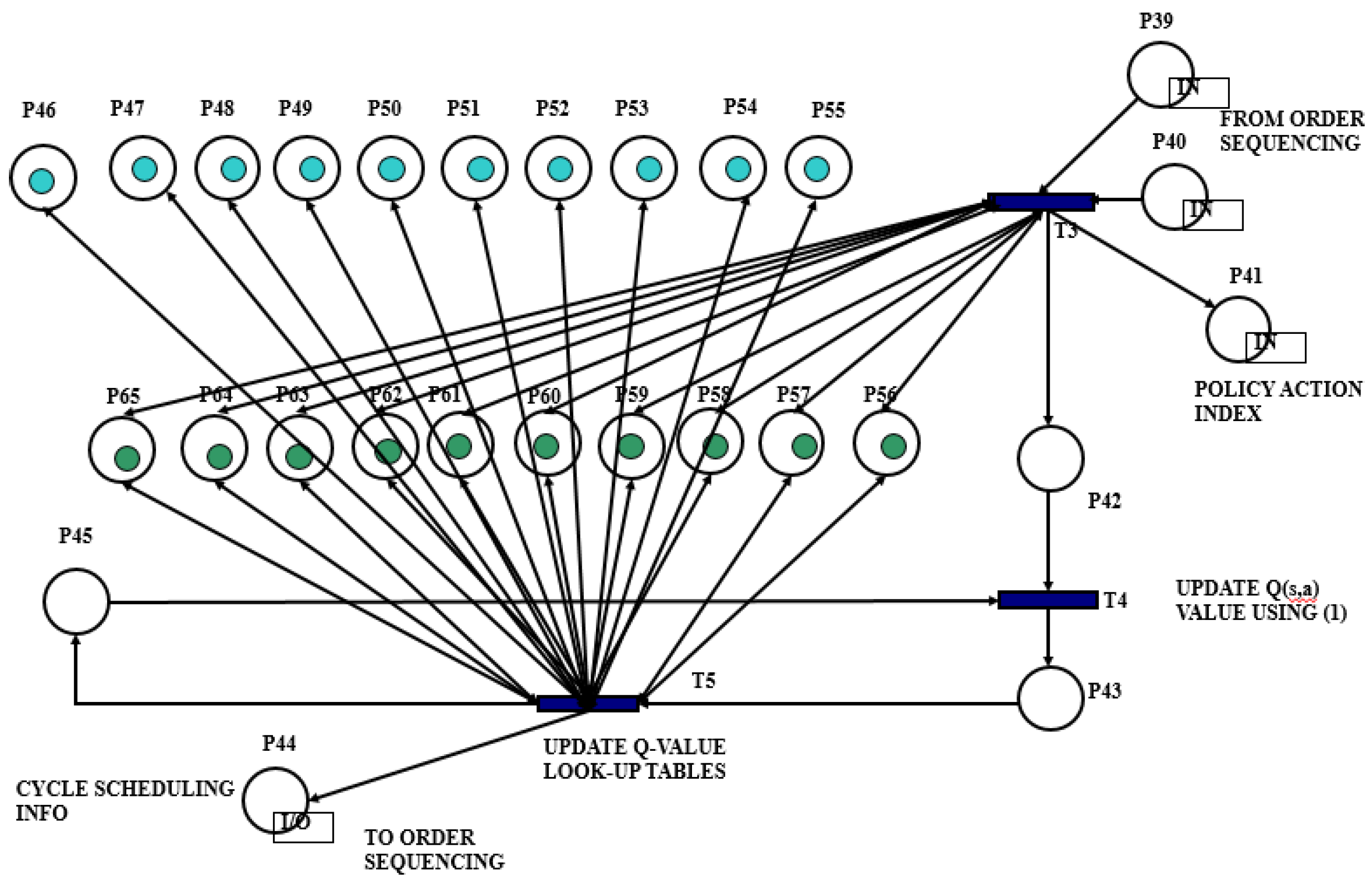
The Q-Learning substitution transition, shown in Figure 6, implements the Q-learning strategy. It contains the look-up tables of Q(s,a) values for states 1 to 10, as color tokens of color set QVAL, a list of REAL, stored in places P46 to P65, corresponding to the available policy state-action pairs (Table 1). The immediate reward and new state tokens are input tokens to the transition T3, stored in places P39 and P40 respectively. T3 fires to calculate the maximum Q-value for the new state, to be used in Equation (1) and the next policy action, held as color tokens in places P42 and P41 respectively. The next policy action token is used as input token to the Order Sequencing substitution transition (held in places P19, P20, and P25 of the Order Sequencing). Transition T4 updates the Q-value of the current state, using Equation (1). Transition T5 updates the tokens in the look-up table places of Q(s,a) values P46 to P65. T5 outputs to the Order Sequencing substitution transition a cycle scheduling information token, held in place P39, a list with the scheduling cycle index or indices corresponding to the terminal dummy environment state. At the end of the 1000 cycles, the Order Sequencing output tokens, held in place P13 and P14 in the Scheduling Agent subnet, are input tokens to the Final Order Sequencing Calculation substitution transition.
Final Order Sequencing Calculation substitution transition finds the minimal total robot travel time for the current batch of orders and retrieves the corresponding cycle index. Using the cycle index value, the corresponding order sequencing is retrieved and transferred to the Scheduling Agent as the final order sequencing, held in places P15 (tote location list) and P16 (compartment location list) (places P4 and P5 in the top scheduling system model page).

5. Simulation and State Space Results

5.1. Validation of the Scheduling Method

Verification of the proposed scheduling method has been done by comparing simulation results for makespan obtained in this study with published literature results. Validation of the method has been supported by the state space results of modeled system properties. The method was tested by applying it to known job shop benchmark examples, i.e., ft6 (six resources and six jobs) [65], as well as the example introduced by Xiong and Zhou [26] with lot sizes (1,1,1,1), (5,5,2,2), and (10,10,6,6). The scheduling goal was to obtain the minimal makespan. A total of 10 states were included. Two dummy states represented the initial state and the terminal state. The terminal state was reached when the obtained makespan was not larger than 5% of the known optimal makespan. The scheduling agent could choose between two possible actions in each state. The first policy action corresponded to a restricted CTPN scheduling model of the benchmark example under investigation, such as the one of the SPT rule, whereas the second policy action was an unrestricted CTPN scheduling model. Each simulation experiment was run for 1000 replications.
Replication results were averaged for each simulation experiment. Simulation results are shown in Table 4. When the Q-learning was implemented with ε = 0 the agent always favored the second policy action, i.e., the unrestricted CTPN scheduling model, except for the first scheduling cycle where the initial condition was guiding it to choose the first policy action. When the agent followed an ε-greedy policy, i.e., a policy with ε = 0.2, it was choosing both policy actions, e.g., in one simulation run of the ft6 benchmark example with ε = 0.2, the best obtained solution was 57, whereas the agent chose the first policy action 97 times and the second policy action 903 times. The first policy action, i.e., the implementation of the SPT rule led to a makespan of 93, whereas the second policy action led to a makespan of 57. The Q-learning algorithm always converged to the optimal solution for the examples introduced in [24]. Τhe best solution obtained for the ft6 benchmark example was 57.
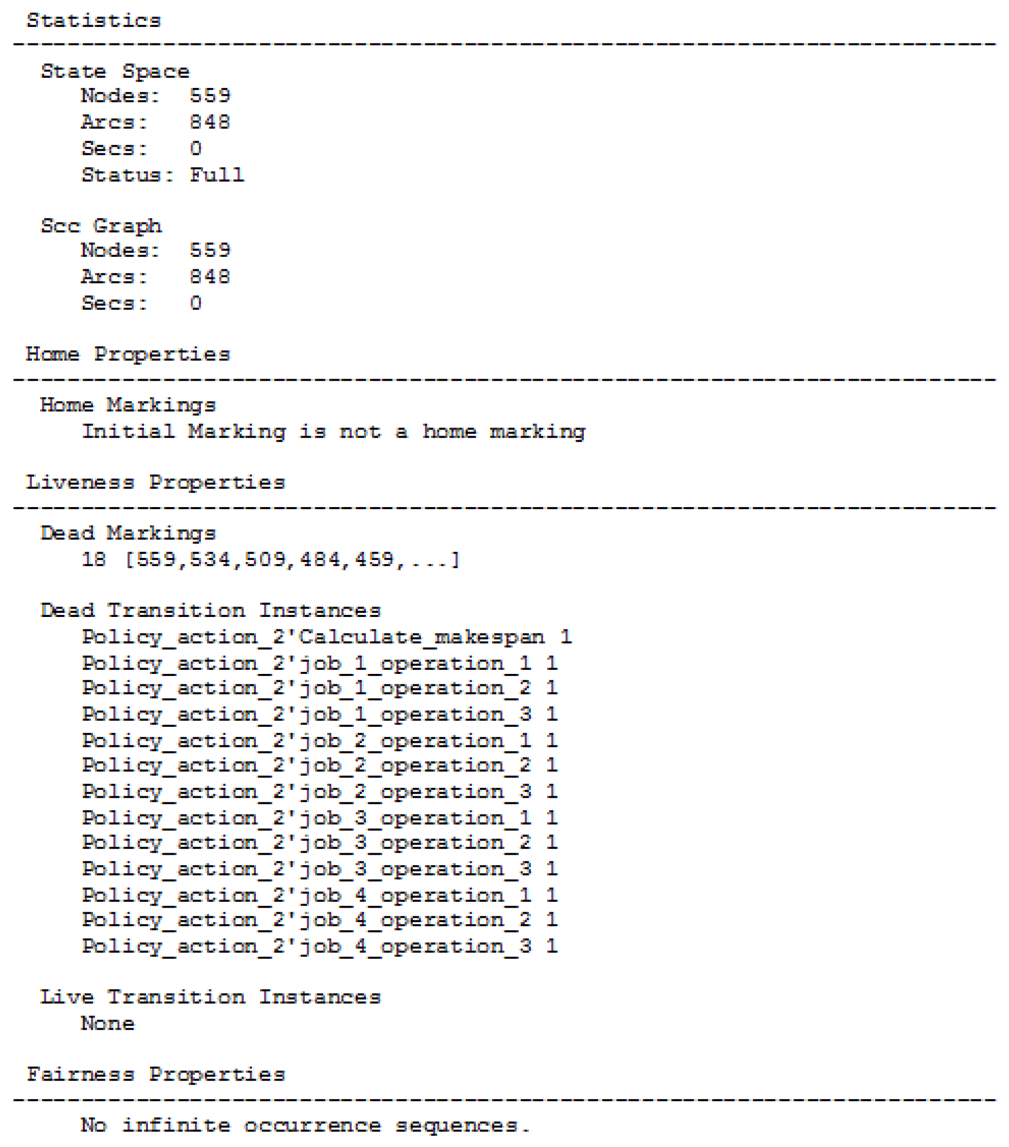
State space was extracted for the CTPN scheduling system model of the job shop example introduced in [26] with lot size (1,1,1,1). One scheduling cycle was taken in the system model. State space analysis results for home, liveness, deadlock exploration, and fairness properties, as well as occurrence graph (OG) (reachability graph) and strongly connected graph (SCC) statistics are shown in Figure 6. Full state space has been calculated. 18 dead markings were identified. Using the OG graph marking information, it was found that all dead markings correspond to the final system state reached when the scheduling was completed. They differ in the combinations of individual job completion times and makespan. Dead transition instances (TIs) are shown in Figure 7. However they correspond to the transitions of the second policy action submodel, i.e., Policy Action 2 submodel in Figure 4. Since the implemented state space system model allowed one scheduling cycle and the initial condition guided the agent to choose the first policy action, the Policy Action 2 subnet was not enabled. When more than one scheduling cycle was included in the model, there were no dead Tis; however the number of dead markings as well as the number of nodes increased. The absence of dead TIs indicates that there are no deadlocks in the system, since a deadlock would appear if a transition could not be enabled, blocking the occurrence of a possible system state. There are no live TIs as well, since there are dead markings. Additionally, there are no infinite occurrence sequences, thus the system always terminates, a result that is further supported by the identical number of nodes and arcs for the state space and SCC graphs. It should be noted that the number of nodes in the presented method, i.e., 559 nodes, is less than the expanded markings (i.e., 598) found in Xiong and Zhou [26].

5.2. Case Study Performance Evaluation

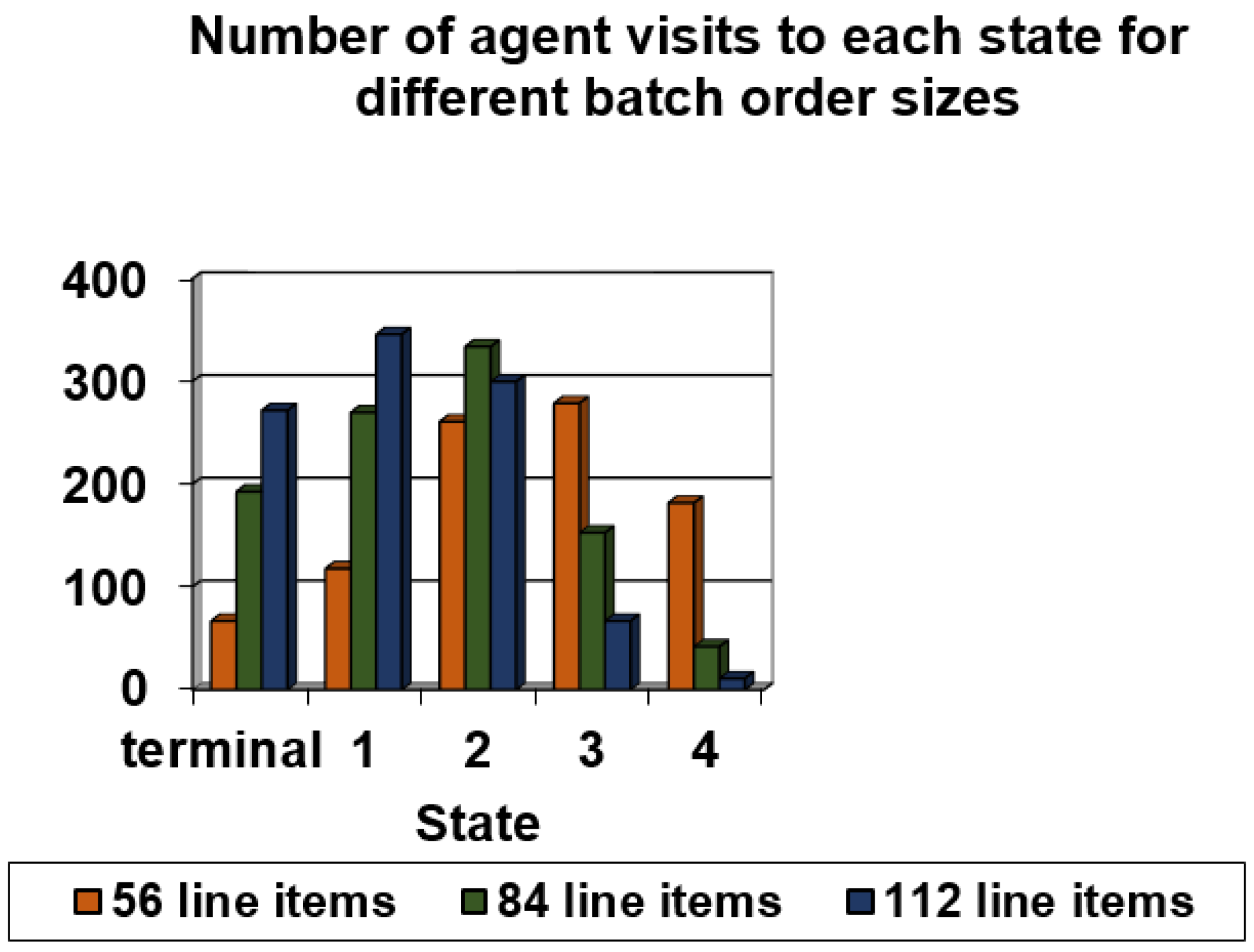
Simulation results were obtained for five batches of 28 orders each, with mean order size (i) twoline item per order; (ii) three line items per order; and (iii) four line items per order. The Q-learning was employed for a training period of 1000 cycles. Each simulation experiment was run for 100 replications. Replication results were averaged for each simulation experiment. Simulation results for the scheduling of the first batch of orders for each considered case are shown in Table 5 and Figure 8. Simulation results in Table 5 show the scheduling rule followed by the agent, the number of agent Q-learning visits to each state, and the total robot travel time, ttot, of the obtained scheduling. Results in Table 5 show that the agent selects the first policy action, i.e., the X-coordinate based heuristic in the considered cases. The X-coordinate based heuristic is expected to yield optimal solutions when the length of each zone is much longer than its width. Thus, the agent was trained to select the action that yields an optimal solution. Figure 8 shows the number of agent visits to each state. Approximate analytical model travel time expressions for a robotic P2B system with randomized storage were presented in Khachatryan and McGinnis [62]. The expected item travel time is bounded by the height in time of the pick zone in the analytical model. For the simulated system this limit is equal to 6 s. The simulated mean item travel time results in Table 5 are close to the 6 s limit. Results in Table 5 indicate that the scheduling agent visits the terminal dummy state, as well as states 1 to 4. It rarely visits higher number states; however, these states were kept in the policy table (Table 1) for different problem cases. The Q-learning converges to an optimal solution in all cases. Results also show that as the mean order size increases the number of agent visits to the terminal state increases during the 1000 cycles.
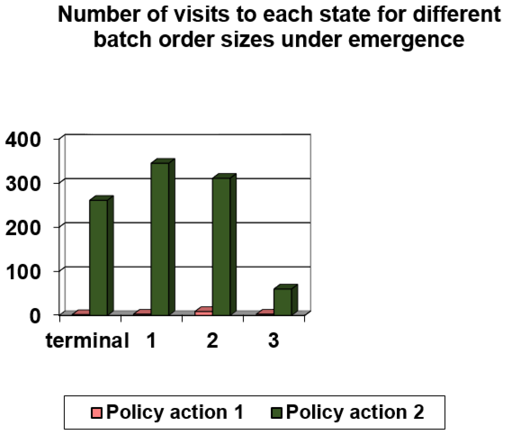
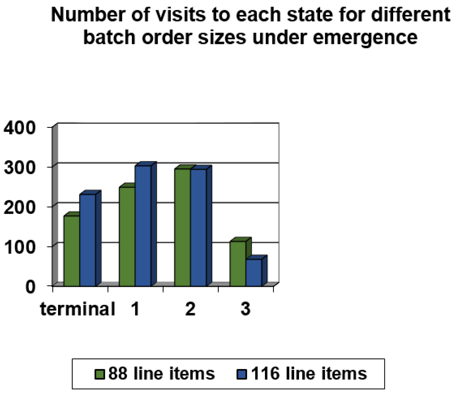
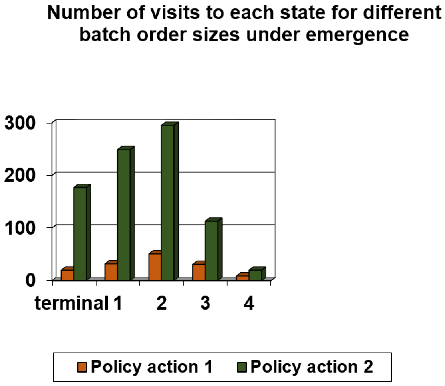
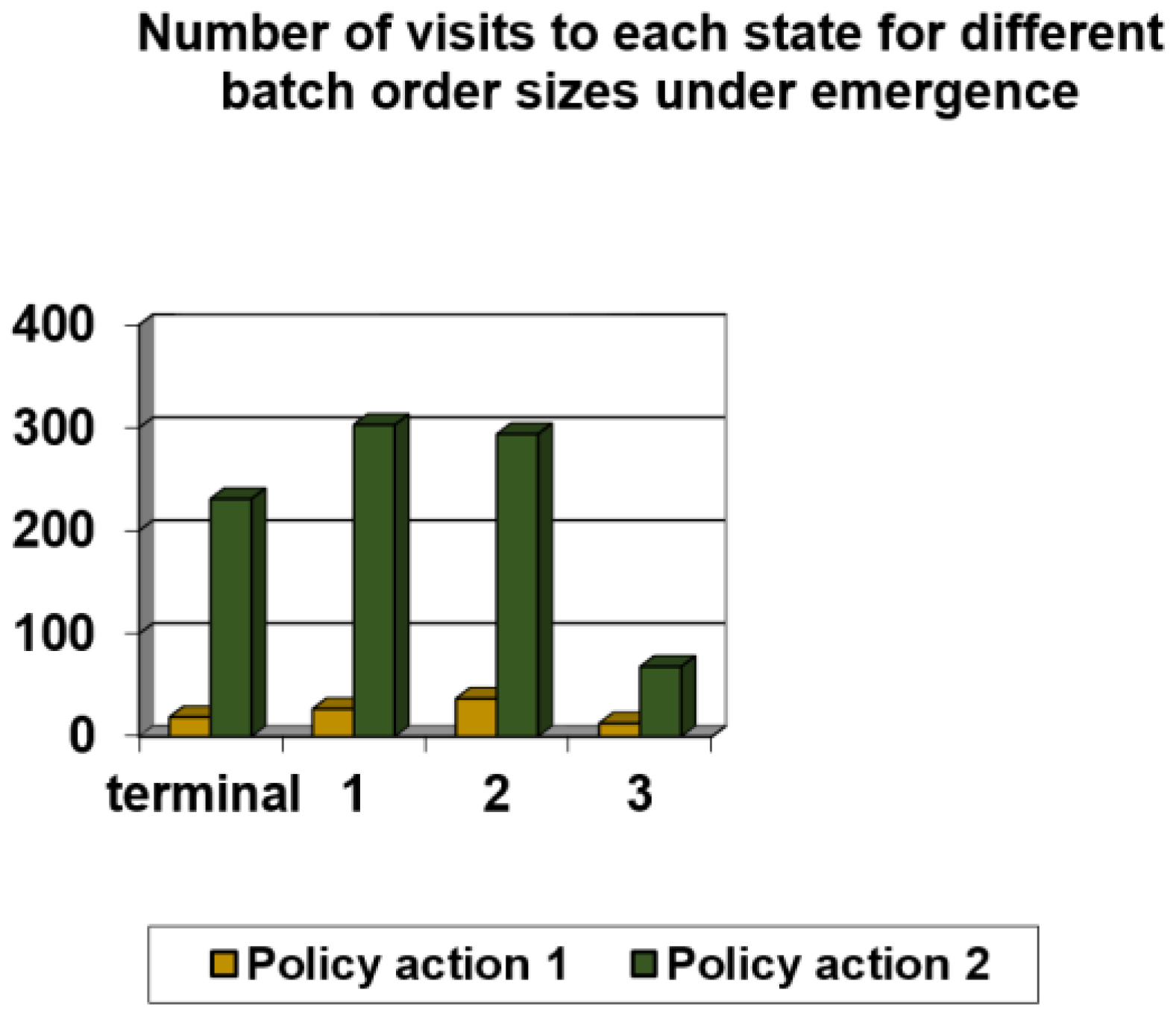
Late order arrival has been considered in order to evaluate the performance of the scheduling method in emergence. Four late orders of one line item each were added to the normal workload of five batches of 28 orders each with mean order size (i) three line items per order; and (ii) four line items per order. The scheduling policy in case of late order arrivals, shown in Table 6, consists of 10 states, and two dummy states. The immediate reward values, shown in Table 7, take into account the total travel time, ttot as well as a balanced workload among robots. The symbol ˄ represents the logic AND operation in Table 6 and Table 7, whereas ttot,roboti , represents the total robot travel time of robot i, i = 1, 2, 3, 4. In each state the agent could select between two actions: (1) to pick all four emergency orders from pick zone 1; or (2) to pick two emergency orders from pick zone 1 and two emergency orders from pick zone 2. The agent followed the X-coordinate based heuristic to implement the order sequencing after the action selection. The Q-learning algorithm was employed by the agent for a training period of 1000 cycles. Each simulation experiment was run for 100 replications. Replication results were averaged for each simulation experiment. Table 8 shows the order picking workload distribution among pick zones, under the different policy actions, for one batch of orders with mean order size 3 line items per order and 4 emergency orders. Simulation results were obtained for different implementations of the Q-learning. In one implementation the scheduling agent fully exploited the Q-learning method, i.e., employed the Q-learning with ε = 0, whereas in a different experiment it followed an ε-greedy policy, with ε = 0.2.
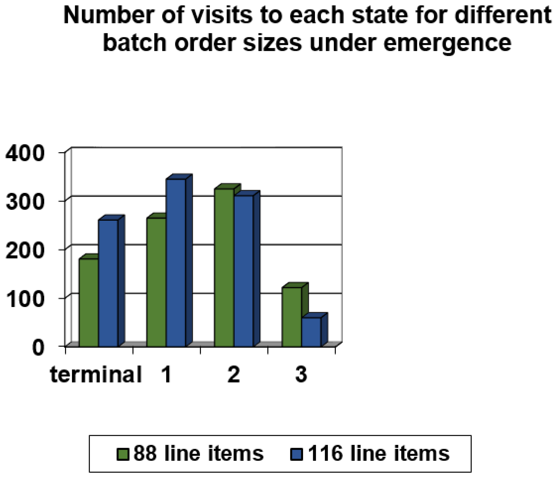
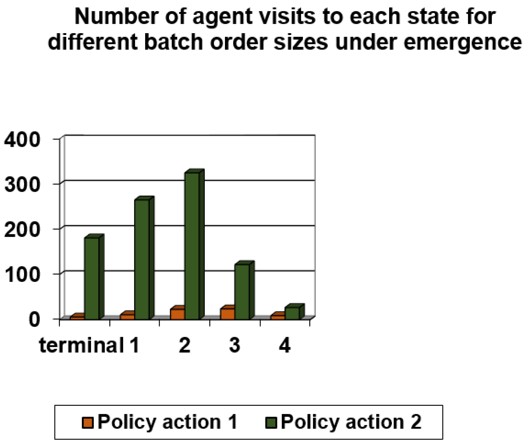
Simulation results for the scheduling of the first batch of orders for each considered case are shown in Table 9 and Figure 9, Figure 10, Figure 11, Figure 12, Figure 13 and Figure 14. Simulation results in Table 9 show the scheduling rule followed by the agent and the number of agent visits to each state for the scheduling of one batch of 28 orders with mean order size three line items per order and four emergency orders. The Q-learning was implemented with ε = 0. Figure 9 shows the number of agent visits to each state for the scheduling of one batch of 28 orders with mean order size (i) three line items per order; and (ii) four line items per order and four emergency orders, when the agent selected the second policy action. The Q-learning was implemented with ε = 0. The results in Table 9 and Figure 9 show that Q-learning converged to an optimal solution in all cases. The agent was trained by the Q-learning to achieve the scheduling goal, i.e., a minimal robot travel time as well as a balanced workload among robots. The balanced workload is better achieved when the agent follows the second policy action (Table 6 and Table 8), thus the agent was trained to achieve the optimal solution, since it favored the second policy action. Figure 10 and Figure 11 show the number of agent visits to each state for the scheduling of one batch of 28 orders with mean order size (i) three line items per order; and (ii) four line items per order and four emergency orders, respectively. Figure 10 shows the results of Table 9. Figure 12, Figure 13 and Figure 14 show similar results to the ones in Figure 9, Figure 10 and Figure 11, where the agent followed an ε-greedy Q-learning strategy with ε = 0.2. Results in Figure 9 and Figure 12 show that the differences in the number of agent visits to each state for different mean order sizes have decreased with the ε-greedy Q-learning strategy. Results from Figure 12, Figure 13 and Figure 14 also indicate that Q-learning converged to an optimal solution in all cases. The agent was trained to achieve the optimal solution, since it favored the second policy action when it followed the ε-greedy Q-learning strategy.
Figure 15 shows the top page of the implemented CTPN model for the scheduling of five batches of 28 orders each with order size of two line items per order. The color tokens show the order sequencing from top to bottom, with the list of tote pick locations and compartment pick locations, as well as the cumulative workload schedule.

6. Conclusions

A manufacturing scheduling method is presented based on hierarchical CTPNs and RL. CTPNs model the system and implement the scheduling. Since the manufacturing scheduling is NP-hard, in the search for an optimal or near-optimal solution a single scheduling agent employs the Q-learning algorithm. The proposed method is an alternative hybrid approach in the context of the complementarity of methods used to handle the scheduling. CPNs can efficiently model the complexity and dynamic behavior of FMS, and evaluate its performance, whereas an intelligent agent with learning capabilities searches for an optimal scheduling solution by using RL. The method does not depend on state space exploration for the scheduling; however, state space analysis can be used to identify and verify system properties. While PNs have been combined with AI techniques in the literature, the potential of the method lies in the exploration, development, and evaluation of the agent’s learning capabilities with respect to the manufacturing scheduling objectives in a CTPN-based modeled system. A warehouse order-picking scheduling is presented as a case study to illustrate the method. The proposed method has been tested under different scheduling objectives. It has been compared to existing methods in order to illustrate its validity and applied to known job shop benchmark examples. Besides simulation results, state space results have supported the validation of the method. State space results have indicated a deadlock-free system model.
The optimal scheduling solution was based on the criteria set in the policy table, i.e., in the model of the environment. The number of state-action pairs, as well as the agent training period number of cycles, influences the state space size as well. State space explosion is a main limitation in PN-based scheduling. Similarly, the large number of environmental states poses limitations in the accuracy of the employed RL method. These parameters can change depending on the case studied.
Future research could explore a distributed scheduling method, in which each resource is linked to its own agent in order to further control the CTPN model execution. Under this scheme, a system state could be defined by the remaining operations for each resource and their precedence relationships, whereas actions could be defined by the set of enabled operations for the resources. The Q-learning would be implemented by each agent in order to obtain an optimal or near optimal solution.

Author Contributions

Maria Drakaki conceived, designed and performed the experiments; Maria Drakaki and Panagiotis Tzionas analyzed the data and prepared the paper.

Conflicts of Interest

The authors declare no conflict of interest.

References

  1. Shen, W.; Wang, L.; Hao, Q. Agent-Based Distributed Manufacturing Process Planning and Scheduling: A State-of the-Art Survey. IEEE Trans. Syst. Man Cybern. 2006, 36, 563–577. [Google Scholar] [CrossRef]
  2. Leitao, P. Agent-based distributed manufacturing control: A state-of-the-art survey. Eng. Appl. Artif. Intell. 2009, 22, 979–991. [Google Scholar] [CrossRef]
  3. Lee, D.Y.; DiCesare, F. Scheduling flexible manufacturing systems using Petri nets and heuristic search. IEEE Trans. Robot. Autom. 1994, 10, 123–133. [Google Scholar] [CrossRef]
  4. Shen, W.; Maturana, F.; Norrie, D.H. Enhancing the performance of an agent-based manufacturing system through learning and forecasting. J. Intell. Manuf. 2000, 11, 365–380. [Google Scholar] [CrossRef]
  5. Wooldridge, M.; Jennings, N.R. Intelligent agents: Theory and practice. Knowl. Eng. Rev. 1995, 10, 115–152. [Google Scholar] [CrossRef]
  6. Sutton, R.S.; Barto, A.G. Reinforcement Learning: An Introduction; The MIT Press: Cambridge, MA, USA, 1999. [Google Scholar]
  7. Watkins, C.J.; Dayan, P. Q-learning. Mach. Learn. 1992, 8, 279–292. [Google Scholar] [CrossRef]
  8. Murata, T. Petri-Nets: Properties, Analysis and Applications. Proc. IEEE. 1989, 77, 541–580. [Google Scholar] [CrossRef]
  9. Reisig, W. Petri Nets: An Introduction. In EATCS Monographs on Theoretical Computer Science; Springer: Berlin/Heidelberg, Germany, 1985. [Google Scholar]
  10. Lin, J.T.; Lee, C.C. A Petri net-based integrated control and scheduling scheme for flexible manufacturing cells. Comput. Integr. Manuf. 1997, 10, 109–122. [Google Scholar] [CrossRef]
  11. Zhou, M.C.; McDermott, K.; Patel, P.A. Petri Net Synthesis and Analysis of a Flexible Manufacturing System Cell. IEEE Trans. Syst. Man. Cybern. 1993, 23, 523–531. [Google Scholar] [CrossRef]
  12. Wu, N. Necessary and Sufficient Conditions for Deadlock-Free Operation in Flexible Manufacturing Systems Using a Colored Petri Net Model. IEEE Trans. Syst. Man Cybern. C 1999, 29, 129–204. [Google Scholar]
  13. Tuncel, G.; Bayhan, G.M. Applications of Petri nets in production scheduling: A review. Int. J. Adv. Manuf. Technol. 2007, 34, 762–773. [Google Scholar] [CrossRef]
  14. Jensen, K.; Kristensen, L.M. Coloured Petri Nets: Modelling and Validation of Concurrent Systems; Springer: Berlin/Heidelberg, Germany, 2009. [Google Scholar]
  15. Narciso, M.E.; Piera, M.A.; Guasch, A. A time stamp reduction method for state space exploration using colored Petri nets. Simulation 2012, 88, 592–616. [Google Scholar] [CrossRef]
  16. Piera, M.A.; Narciso, M.; Guasch, A.; Riera, D. Optimization of logistic and manufacturing systems through simulation: A colored Petri net-based methodology. Simulation 2004, 80, 121–130. [Google Scholar] [CrossRef]
  17. Moore, K.E.; Gupta, S.M. Petri net models of flexible and automated manufacturing systems: A survey. Int. J. Prod. Res. 1996, 34, 3001–3035. [Google Scholar] [CrossRef]
  18. Hatano, I.; Yamagata, K.; Tamura, H. Modeling and on-line scheduling of flexible manufacturing systems using stochastic Petri nets. IEEE Trans. Softw. Eng. 1991, 17, 126–133. [Google Scholar] [CrossRef]
  19. Camurri, A.; Franchi, P.; Gandolfo, F.; Zaccaria, R. Petri net based process scheduling: A model of the control system of flexible manufacturing systems. J. Intell. Robot. Syst. 1993, 8, 99–123. [Google Scholar] [CrossRef]
  20. Chiola, G.; Dutheillet, C.; Franceschinis, G.; Haddad, S. Stochastic well-formed colored nets and symmetric modeling applications. IEEE Trans. Comput. 1993, 42, 1343–1360. [Google Scholar] [CrossRef]
  21. Castiglione, A.; Gribaudo, M.; Iacono, M.; Palmieri, F. Modeling performances of concurrent big data applications. Softw. Pract. Exp. 2015, 45, 1127–1144. [Google Scholar] [CrossRef]
  22. Shih, H.; Sekiguchi, T. A timed Petri net and beam search based on-line FMS scheduling system with routing flexibility. In Proceedings of the 1991 IEEE International Conference on Robotics and Automation, Sacramento, CA, USA, 1991; pp. 2548–2553.
  23. Chen, Q.; Luh, J.Y.S.; Shen, L. Complexity reduction for optimization of deterministic timed Petri-net scheduling by truncation. Cybern. Syst. 1994, 25, 643–695. [Google Scholar] [CrossRef]
  24. Zhou, M.C.; Xiong, H.H. Petri net scheduling of FMS using branch-and-bound method. In Proceedings of the 1995 IEEE International Conference on Industrial Electronics, Control, and Instrumentation, Orlando, FL, USA, 6–10 November 1995; pp. 211–216.
  25. Sun, T.H.; Cheng, C.W.; Fu, L.C. Petri net based approach to modeling and scheduling for an FMS and a case study. IEEE Trans. Ind. Electron. 1994, 41, 593–601. [Google Scholar]
  26. Xiong, H.H.; Zhou, M.C. Scheduling of semiconductor test facility via Petri nets and hybrid heuristic search. IEEE Trans. Semicond. Manuf. 1998, 11, 384–393. [Google Scholar] [CrossRef]
  27. Jeng, M.D.; Chen, S.C. Heuristic search approach using approximate solutions to Petri net state equations for scheduling flexible manufacturing systems. Int. J. Flex. Manuf. Syst. 1998, 10, 139–162. [Google Scholar] [CrossRef]
  28. Jeng, M.D.; Lin, C.S.; Huang, Y.S. Petri net dynamics-based scheduling of flexible manufacturing systems with assembly. J. Intell. Manuf. 1999, 10, 541–555. [Google Scholar] [CrossRef]
  29. Reyes, A.; Yu, H.; Kelleher, G.; Lloyd, S. Integrating Petri Nets and hybrid heuristic search for the scheduling of FMS. Comput. Ind. 2002, 47, 123–138. [Google Scholar] [CrossRef]
  30. Yu, H.; Reyes, A.; Cang, S.; Lloyd, S. Combined Petri nets modelling and AI-based heuristic hybrid search for flexible manufacturing systems-part II. Heuristic hybrid search. Comput. Ind. Eng. 2003, 44, 545–566. [Google Scholar] [CrossRef]
  31. Mejía, G.; Odrey, N.G. An approach using Petri Nets and improved heuristic search for manufacturing system scheduling. J. Manuf. Syst. 2005, 24, 79–92. [Google Scholar] [CrossRef]
  32. Lee, J.; Lee, J.S. Heuristic search for scheduling flexible manufacturing systems using lower bound reachability matrix. Comput. Ind. Eng. 2010, 59, 799–806. [Google Scholar] [CrossRef]
  33. Huang, B.; Jiang, R.; Zhang, G. Search strategy for scheduling flexible manufacturing systems simultaneously using admissible heuristic functions and nonadmissible heuristic functions. Comput. Ind. Eng. 2014, 71, 21–26. [Google Scholar] [CrossRef]
  34. Kim, Y.W.; Suzuki, T.; Narikiyo, T. FMS scheduling based on timed Petri Net model and reactive graph search. Appl. Math. Model. 2007, 31, 955–970. [Google Scholar] [CrossRef]
  35. Mejía, G.; Montoya, C. A Petri net based algorithm for scheduling manufacturing systems with blocking. Int. J. Prod. Res. 2009, 47, 6261–6277. [Google Scholar] [CrossRef]
  36. Odrey, N.; Mejia, G. An augmented Petri net approach for error recovery in manufacturing systems control. Robot. Comput. Integr. Manuf. 2005, 21, 346–354. [Google Scholar] [CrossRef]
  37. Murata, T.; Nelson, P.C.; Yim, J. A predicate-transition net model for multiple agent planning. Inf. Sci. 1991, 57, 361–384. [Google Scholar] [CrossRef]
  38. Leitao, P.; Colombo, A.W.; Restivo, F. An approach to the formal specification of holonic control systems. In Lecture Notes in Computer Science, Holonic and Multi-Agent Systems for Manufacturing, Proceedings of the First International Conference on Industrial Applications of Holonic and Multi-Agent Systems, Prague, Czech Republic, 1–3 September 2003; Springer: Berlin/Heidelberg, Germany, 2003; Volume 2744, pp. 59–70. [Google Scholar]
  39. Hsieh, F.S. Model and control holonic manufacturing systems based on fusion of contract nets and petri nets. Automatica 2004, 40, 51–57. [Google Scholar] [CrossRef]
  40. Giglio, D.; Paolucci, M. Agent-based Petri net models for AGV management in manufacturing systems. In Proceedings of the IEEE International Conference on Systems, Man, and Cybernetics, Tucson, AZ, USA, 7–10 October 2001; Volume 4, pp. 2457–2462.
  41. Castelnuovo, A. Petri net models of agent-based control of a FMS with randomly generated recipes. In Proceedings of the 10th IEEE Conference on Emerging Technologies and Factory Automation, Catania, Italy, 19–22 September 2005; Volume 1, pp. 935–942.
  42. Bai, Q.; Ren, F.; Zhang, M.; Fulcher, J. CPN-Based State Analysis and Prediction for Multi-agent Scheduling and Planning. In Advances in Agent-Based Complex Automated Negotiations, Studies in Computational Intelligence; Ito, T., Zhang, M., Robu, V., Fatima, S., Matsuo, T., Eds.; Springer: Berlin/Heidelberg, Germany, 2009; Volume 233, pp. 161–176. [Google Scholar]
  43. Demongodin, I.; Hennet, J.C. A Petri net model of distributed control in a holonic Manufacturing Execution System. In Proceedings of the 17th World Congress, the International Federation of Automatic Control, Seoul, Korea, 6–11 July 2008; pp. 6–11.
  44. Drakaki, M.; Tzionas, P. Modeling and performance evaluation of an agent-based warehouse dynamic resource allocation using Colored Petri Nets. Int. J. Comput. Integr. Manuf. 2016, 29, 736–753. [Google Scholar] [CrossRef]
  45. Huang, G.Y. Analysis of Artificial Intelligence Based Petri Net Approach to Intelligent Integration of Design. In Proceedings of the IEEE International Conference on Machine Learning and Cybernetics, Dalian, China, 13–16 August 2006; pp. 1691–1695.
  46. Chen, S.M.; Ke, J.S.; Chang, J.F. Knowledge representation using fuzzy Petri nets. IEEE Trans. Knowl. Data Eng. 1990, 2, 311–319. [Google Scholar] [CrossRef]
  47. Joseph, J. Petri nets and the application to artificial intelligence. In Proceedings of the IEEE Colloquium on Software Engineering Practices for Intelligent Knowledge-Based Systems, London, UK, 17 March 1989; pp. 411–414.
  48. Zha, X.F.; Lim, S.Y.; Fok, S.C. Concurrent intelligent design and assembly planning: Object-oriented intelligent Petri nets approach. In Proceedings of the 1997 IEEE Conference on Systems, Man, and Cybernetics, Orlando, FL, USA, 12–15 October 1997; pp. 30–39.
  49. Zha, X.F.; Lim, S.Y.E.; Fok, S.C. Integration of knowledge-based systems and neural networks: Neuro-expert Petri net models and applications. In Proceedings of the 1998 IEEE International Conference on Robotics and Automation, Leuven, Belgium, 16–21 May 1998.
  50. Jávor, A. Petri nets and AI in modeling and simulation. Math. Comput. Simul. 1995, 39, 477–484. [Google Scholar] [CrossRef]
  51. Aydin, M.E.; Oztemel, E. Dynamic job-shop scheduling using reinforcement learning agents. Robot. Auton. Syst. 2000, 33, 169–178. [Google Scholar] [CrossRef]
  52. Russell, S.; Norvig, P. Artificial Intelligence: A Modem Approach; Prentice-Hall: Englewood Cliffs, NJ, USA, 1995. [Google Scholar]
  53. Wang, Y.C.; Usher, J.M. Application of reinforcement learning for agent-based production scheduling. Eng. Appl. Artif. Intell. 2005, 18, 73–82. [Google Scholar] [CrossRef]
  54. Zhang, W.; Dietterich, T.G. A reinforcement learning approach to job-shop scheduling. In Proceedings of the 14th International Joint Conference on Artificial Intelligence, Montreal, QC, Canada, 20–25 August 1995; pp. 1114–1120.
  55. Mahadevan, S.; Marchalleck, N.; Das, T.K.; Gosavi, A. Self-improving factory simulation using continuous-time average reward reinforcement learning. In Proceedings of the 14th International Machine Learning Conference, Nashville, TN, USA, 8–12 July 1997; pp. 202–210.
  56. Das, T.K.; Gosavi, A.; Mahadevan, S.; Marchalleck, N. Solving semi-Markov decision problems using average reward reinforcement learning. Manag. Sci. 1999, 45, 560–574. [Google Scholar] [CrossRef]
  57. Mahadevan, S.; Theocharous, G. Optimizing production manufacturing using reinforcement learning. In Proceedings of the Eleventh International FLAIRS Conference, Sanibel Island, FL, USA, 18–20 May 1998; pp. 372–377.
  58. Paternina-Arboleda, C.D.; Das, T.K. Intelligent dynamic control policies for serial production lines. IIE Trans. 2001, 33, 65–77. [Google Scholar] [CrossRef]
  59. Paternina-Arboleda, C.D.; Das, T.K. A multi-agent reinforcement learning approach to obtaining dynamic control policies for stochastic lot scheduling problem. Simul. Model. Pract. Theory 2005, 13, 389–406. [Google Scholar] [CrossRef]
  60. Gabel, T.; Riedmiller, M. Adaptive reactive job-shop scheduling with reinforcement learning agents. Int. J. Inf. Technol. Intell. Comput. 2008, 24. [Google Scholar]
  61. Csáji, B.C.; Monostori, L.; Kádár, B. Reinforcement learning in a distributed market-based production control system. Adv. Eng. Inform. 2006, 20, 279–288. [Google Scholar] [CrossRef]
  62. Khachatryan, M.; McGinnis, L.F. Picker Travel Time Model for an Order Picking System with Buffers. IIE Trans. 2014, 46, 894–904. [Google Scholar] [CrossRef]
  63. Kim, B.; Graves, R.J.; Heragu, S.S.; Onge, A.S. Intelligent agent modeling of an industrial warehousing problem. IIE Trans. 2002, 34, 601–612. [Google Scholar] [CrossRef]
  64. Jensen, K.; Kristensen, L.M.; Wells, L. Coloured Petri Nets and CPN Tools for modelling and validation of concurrent systems. Int. J. Softw. Tools Technol. Trans. 2007, 9, 213–254. [Google Scholar] [CrossRef]
  65. Fisher, H.; Thompson, G.L. Probabilistic learning combinations of local job-shop scheduling rules. In Industrial Scheduling; Muth, J.F., Thompson, G.L., Eds.; Prentice-Hall: Englewood Cliffs, NJ, USA, 1963; pp. 225–251. [Google Scholar]
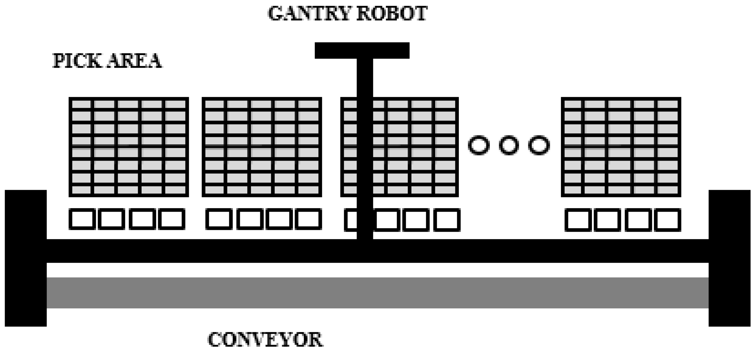
Figure 1. The layout of a pick zone.
Applsci 07 00136 g001
Figure 2. The top page of the implemented hierarchical CTPN model of the scheduling system.
Applsci 07 00136 g002
Figure 3. The implemented hierarchical CTPN model of the Scheduling Agent substitution transition.
Applsci 07 00136 g003
Figure 4. The implemented hierarchical CTPN model of the Order Sequencing substitution transition.
Applsci 07 00136 g004
Figure 5. The implemented hierarchical CTPN model of the Perception substitution transition.
Applsci 07 00136 g005
Figure 6. The CTPN model of the Q-Learning substitution transition.
Applsci 07 00136 g006
Figure 7. State space results for the CTPN scheduling system model of the job shop example introduced in [26] with lot size (1,1,1,1), implemented with one scheduling cycle.
Applsci 07 00136 g007
Figure 8. The number of agent visits to each state for the scheduling of one batch of 28 orders, with mean order size (i) two line items per order; (ii) three line items per order; and (ii) four line items per order.
Applsci 07 00136 g008
Figure 9. The number of agent visits to each state for the scheduling of one batch of 28 orders and four emergency orders, with mean order size (i) three line items per order; and (ii) four line items per order, when the agent selected the second policy action. The agent followed a non-ε-greedy policy with ε = 0.
Applsci 07 00136 g009
Figure 10. The number of agent visits to each state for the scheduling of one batch of 28 orders and four emergency orders, with mean order size three line items per order. The agent followed a non-ε-greedy policy with ε = 0.
Applsci 07 00136 g010
Figure 11. The number of agent visits to each state for the scheduling of one batch of 28 orders and four emergency orders, with mean order size four line items per order. The agent followed a non-ε-greedy policy with ε = 0.
Applsci 07 00136 g011
Figure 12. The number of agent visits to each state for the scheduling of one batch of 28 orders and four emergency orders, with mean order size (i) three line items per order; and (ii) four line items per order, when the agent selected the second policy action. The agent followed an ε-greedy policy with ε = 0.2.
Applsci 07 00136 g012
Figure 13. The number of agent visits to each state for the scheduling of one batch of 28 orders and four emergency orders, with mean order size three line items per order. The agent followed an ε-greedy policy with ε = 0.2.
Applsci 07 00136 g013
Figure 14. The number of agent visits to each state for the scheduling of one batch of 28 orders and four emergency orders, with mean order size four line items per order. The agent followed an ε-greedy policy with ε = 0.2.
Applsci 07 00136 g014
Figure 15. Top page of the implemented CTPN model for the scheduling of five batches of 28 orders each with order size of two line items per order. The color tokens show the order sequencing from top to bottom, with the list of tote pick locations and compartment pick locations, as well as the cumulative workload schedule.
Applsci 07 00136 g015
Table 1. Policy table for the scheduling agent.
StateState DefinitionX-Coordinate Based Heuristic-Q(s,a) PairRandom Pick Location Selection-Q(s,a) Pair
DummyInitial state: total robot travel time (ttot) = 000
DummyTerminal state:0.98 × ttot,aver ≤ ttot ≤ 1.02 × ttot,aver00
10.95 × ttot,aver ≤ ttot ≤ 1.05 × ttot,averQ(1,1)Q(2,1)
20.9 × ttot,aver ≤ ttot ≤ 1.1 × ttot,averQ(2,1)Q(2,2)
30.85 × ttot,aver ≤ ttot ≤ 1.15 × ttot,averQ(3,1)Q(3,2)
40.8 × ttot,aver ≤ ttot ≤ 1.2 × ttot,averQ(4,1)Q(4,2)
50.75 × ttot,aver ≤ ttot ≤ 1.25 × ttot,averQ(5,1)Q(5,2)
60.7 × ttot,aver ≤ ttot ≤ 1.3 × ttot,averQ(6,1)Q(6,2)
70.65 × ttot,aver ≤ ttot ≤ 1.35 × ttot,averQ(7,1)Q(7,2)
80.6 × ttot,aver ≤ ttot ≤ 1.4 × ttot,averQ(8,1)Q(8,2)
90.55 × ttot,aver ≤ ttot ≤ 1.45 × ttot,averQ(9,1)Q(9,2)
100.55 × ttot,aver > ttot, ttot > 1.45 × ttot,averQ(10,1)Q(10,2)
Table 2. Immediate reward (r) values.
If 0.95 × ttot,aver ≤ ttot ≤ 1.05 × ttot,aver then r = 4.5
If 0.9 × ttot,aver ≤ ttot ≤ 1.1 × ttot,aver then r = 4.0
If 0.85 × ttot,aver ≤ ttot ≤ 1.15 × ttot,aver then r = 3.0
If 0.8 × ttot,aver ≤ ttot ≤ 1.2 × ttot,aver then r = 2.5
If 0.75 × ttot,aver ≤ ttot ≤ 1.25 × ttot,aver then r = 2.0
If 0.7 × ttot,aver ≤ ttot ≤ 1.3 × ttot,aver then r = 1.0
If 0.65 × ttot,aver ≤ ttot ≤ 1.35 × ttot,aver then r = −1.0
If 0.6 × ttot,aver ≤ ttot ≤ 1.4 × ttot,aver then r = −2.0
If 0.55 × ttot,aver ≤ ttot ≤ 1.45 × ttot,aver then r = −3.0
If 0.55 × ttot,aver > ttot, ttot > 1.45 × ttot,aver then r = −4.0
Table 3. Basic color set declarations of the CTPN system model.
colset INTT = INT timed; colset REALT = real timed;
colset Order = record orderno:INT*prodno:INT*itemno:INT*AT:INT;
colset ORDER_STREAM = list Order timed;
colset ORDER_SCHEDULE = list ORDER_STREAM;
colset ORIGWORKLDn = record robot1:INT*wkld1:INT*robot2:INT*wkld2:INT*
robot3:INT*wkld3:INT*robot4:INT*wkld4:INT;
colset ORIGWORKLD_SCHEDULE = list ORIGWORKLDn;
colset BATCH_INFO = record batch_ord:INT*batch_wkld: ORDER_STREAM* batch_itm_cnt:INT;
colset BATCH_LIST = list BATCH_INFO;
colset ORDERinBATCH = record orderid:INT*prodno:INT*lnitmno:INT*pickzono:INT;
colset BATCH_of_ORDERS = list ORDERinBATCH;
colset ORDER_STREAM_SCHEDULE = list BATCH_of_ORDERS;
colset PZ1_LOC_LIST = list INT timed;
colset TOTE_LOC_LIST = PZ1_LOC_LISTxPZ2_LOC_LISTxPZ3_LOC_LISTxPZ4_LOC_LIST;
colset COMPT_LOC_LIST = PZ1_LOC_LISTxPZ2_LOC_LISTxPZ3_LOC_LISTxPZ4_LOC_LIST;
colset QVAL = list REAL timed;
colset CYCLE_SCHEDULE_INFO = list REALxINTxREALxREALxREALxREAL;
Table 4. Simulation comparison results for the makespan of job shop benchmark examples. The number in parentheses corresponds to the percentage of the scheduling agent Q-learning visits to the best obtained solution in 1000 cycles, i.e., in one simulation experiment.
Benchmark ExampleOptimal MakespanXiong and Zhou [26]Huang et al. [33]Yu et al. [30]Gabel and Riedmiller [60]This Study
Xiong and Zhou (1998)-lot size (1,1,1,1) [26]17171717-17 (50%)
Xiong and Zhou (1998)-lot size (5,5,2,2) [26]58585858-58 (52%)
Xiong and Zhou (1998)-lot size (10,10,6,6) [26]134134134134-134 (42%)
Fisher and Thompson (1963)-ft6 6x6 [65]55---5757 (0.1%)
Table 5. Simulation results for the scheduling of one batch of 28 orders, with mean order size (i) 2 line item per order; (ii) 3 line items per order; and (iii) 4 line items per order. The number in parentheses shows the calculated average total robot travel time, ttot,aver, from 1000 simulation replications.
Total Number of Line Items in BatchPolicy ActionNumber of Visits to Terminal StateNumber of Visits to State 1Number of Visits to State 2Number of Visits to State 3Number of Visits to State 4Total Robot Travel Time, ttot, (ttot,aver)
56 line items167118261279182341.84 (340.92)
84 line items119327033415342514.14 (513.68)
112 line items12723463006711685.18 (684.72)
Table 6. Policy table for the scheduling agent.
StateState Definition4 Late Orders Assigned to Robot 1 —Q(s,a) Pair2 Late Orders Assigned to Robot 1 and 2 Late Orders to Robot 2 —Q(s,a) Pair
DummyInitial state: total robot travel time (ttot) = 000
DummyTerminal state: 0.85 × ttot,aver ≤ ttot,robot1 ˄ ttot,robot2 ˄ ttot,robot3 ˄ ttot,robot4 ≤ 1.15 × ttot,aver00
10.8 × ttot,aver ≤ ttot,robot1 ˄ ttot,robot2 ˄ ttot,robot3 ˄ ttot,robot4 ≤ 1.2 × ttot,averQ(1,1)Q(2,1)
20.75 × ttot,aver ≤ ttot,robot1 ˄ ttot,robot2 ˄ ttot,robot3 ˄ ttot,robot4 ≤ 1.25 × ttot,averQ(2,1)Q(2,2)
30.7 × ttot,aver ≤ ttot,robot1 ˄ ttot,robot2 ˄ ttot,robot3 ˄ ttot,robot4 ≤ 1.3 × ttot,averQ(3,1)Q(3,2)
40.65 × ttot,aver ≤ ttot,robot1 ˄ ttot,robot2 ˄ ttot,robot3 ˄ ttot,robot4 ≤ 1.35 × ttot,averQ(4,1)Q(4,2)
50.6 × ttot,aver ≤ ttot,robot1 ˄ ttot,robot2 ˄ ttot,robot3 ˄ ttot,robot4 ≤ 1.4 × ttot,averQ(5,1)Q(5,2)
60.55 × ttot,aver ≤ ttot,robot1 ˄ ttot,robot2 ˄ ttot,robot3 ˄ ttot,robot4 ≤ 1.45 × ttot,averQ(6,1)Q(6,2)
70.5 × ttot,aver ≤ ttot,robot1 ˄ ttot,robot2 ˄ ttot,robot3 ˄ ttot,robot4 ≤ 1.5 × ttot,averQ(7,1)Q(7,2)
80.45 × ttot,aver ≤ ttot,robot1 ˄ ttot,robot2 ˄ ttot,robot3 ˄ ttot,robot4 ≤ 1.55 × ttot,averQ(8,1)Q(8,2)
90.4 × ttot,aver ≤ ttot,robot1 ˄ ttot,robot2 ˄ ttot,robot3 ˄ ttot,robot4 ≤ 1.6 × ttot,averQ(9,1)Q(9,2)
100.4 × ttot,aver > ttot,robot1 ˄ ttot,robot2 ˄ ttot,robot3 ˄ ttot,robot4, ttot,robot1 ˄ ttot,robot2 ˄ ttot,robot3 ˄ ttot,robot4 > 1.6 × ttot,averQ(10,1)Q(10,2)
Table 7. Immediate reward (r) values.
If 0.85 × ttot,aver ≤ ttot,robot1 ˄ ttot,robot2 ˄ ttot,robot3 ˄ttot,robot4 ≤ 1.15 × ttot,aver then r = 4.5
If 0.8 × ttot,aver ≤ ttot,robot1 ˄ ttot,robot2 ˄ ttot,robot3 ˄ ttot,robot4 t ≤ 1.2 × ttot,aver then r = 4.0
If 0.75 × ttot,aver ≤ ttot,robot1 ˄ ttot,robot2 ˄ ttot,robot3 ˄ ttot,robot4 ≤ 1.25 × ttot,aver then r = 3.0
If 0.7 × ttot,aver ≤ ttot,robot1 ˄ ttot,robot2 ˄ ttot,robot3 ˄ ttot,robot4 ≤ 1.3 × ttot,aver then r = 2.5
If 0.65 × ttot,aver ≤ ttot,robot1 ˄ ttot,robot2 ˄ ttot,robot3 ˄ ttot,robot4 ≤ 1.35 × ttot,aver then r = 2.0
If 0.6 × ttot,aver ≤ ttot,robot1 ˄ ttot,robot2 ˄ ttot,robot3 ˄ ttot,robot4 ≤ 1.4 × ttot,aver then r = 1.0
If 0.55 × ttot,aver ≤ ttot,robot1 ˄ ttot,robot2 ˄ ttot,robot3 ˄ ttot,robot4 ≤ 1.45 × ttot,aver then r = −1.0
If 0.5 × ttot,aver ≤ ttot,robot1 ˄ ttot,robot2 ˄ ttot,robot3 ˄ ttot,robot4 ≤ 1.5 × ttot,aver then r = −2.0
If 0.45 × ttot,aver ≤ ttot,robot1 ˄ ttot,robot2 ˄ ttot,robot3 ˄ ttot,robot4 ≤ 1.55 × ttot,aver then r = −3.0
If 0.45 × ttot,aver > ttot,robot1 ˄ ttot,robot2 ˄ ttot,robot3 ˄ ttot,robot4, ttot,robot1 ˄ ttot,robot2 ˄ ttot,robot3 ˄ ttot,robot4 > 1.55 × ttot,aver then r = −4.0
Table 8. Order picking workload distribution (number of orders per pick zone) among pick zones under emergence, for the different policy actions, for one batch of 28 orders with mean order size three line items per order and four emergency orders. Workload distribution under normal conditions (i.e., in the absence of emergency orders) has been included.
Scheduling RulePick Zone 1Pick Zone 2Pick Zone 3Pick Zone 4Number of Orders per Pick Zone under Normal Conditions
Policy action 12521212121
Policy action 22323212121
Table 9. Simulation results for the scheduling under emergence of one batch of 28 orders with mean order size three line items per order and four emergency orders. Q-learning was implemented with ε = 0.
Scheduling RuleNumber of Visits to Terminal StateNumber of Visits to State 1Number of Visits to State 2Number of Visits to State 3Number of Visits to State 4Number of Visits to State 5
Policy action 1611232491
Policy action 2181265325122274