A Novel Denoising Method for an Acoustic-Based System through Empirical Mode Decomposition and an Improved Fruit Fly Optimization Algorithm

Abstract

Generally, the sound signal produced by transmission unit or cutting unit contains abundant information about the working state of a machine. The acoustic-based diagnosis system presents some distinct advantages in some severe conditions particularly due to its unique non-contact measurement and unlimited use at the installation site. However, the original acoustic signal collected from manufacture process is always polluted by various background noises. In order to eliminate noise components from machinery sound effectively, an empirical mode decomposition (EMD) threshold denoising method optimized by an improved fruit fly optimization algorithm (IFOA) is launched in this paper. The acoustic signal was first decomposed by the adaptive EMD to obtain a series of intrinsic mode functions (IMFs). Then, the soft threshold function was applied to shrink the IMF coefficients. While the threshold of each IMF was determined by statistical estimation and empirical value for traditional EMD denoising, the denoising effect was often not desired and time-consuming. To solve these disadvantages, fruit fly optimization algorithm (FOA) was introduced to search global optimal threshold of each IMF. Moreover, to enhance the group diversity during production of the next generation of fruit flies and balance the local and global searching ability, a variation coefficient and a disturbance coefficient was introduced to the basic FOA. Then, a piece of simulated acoustic signal produced by the train was applied to validate the proposed EMD and IFOA threshold denoising (EMD-IFOA). The simulation results, which decreased 35.40% and 18.92% in mean squared error (MSE) and percent root mean square difference (PRD) respectively, and increased 40.36% in signal-to-noise ratio improvement (SNR_imp) compared with basic EMD denoising scheme at SNR = 5 dB, illustrated the effectiveness and superiority of the proposed approach. Finally, the proposed EMD-IFOA was conducted on an actual acoustic-based diagnosis system for cutting state recognition of the coal mining shearer to demonstrate the practical effect.

1. Introduction

Over the last years, customers who have wanted to monitor the real-time running condition of the machine’s working process have studied and developed various monitoring methods. An important difference in these methodologies can be summarized as the different measuring system. Generally, the machine monitoring system can be classified as utilizing either contact or non-contact measurement. Contact approaches are mainly aimed at vibration and strain signals to collect dynamic information, however, carrying out of such methods bears the disadvantages of limited detecting positions, which are strict with respect to the measuring directions, and have difficult-to-maintain detectors in some severe situations [1]. Non-contact methods such as acoustic-based, image-based and laser vibrometry-based systems, however, can be used conveniently and do not affect the machine, thereby increasing efficiency and allowing online supervisory control [2,3,4]. The acoustic signal has attracted much attention in industrial monitoring due to its strong robustness to illumination intensity, air quality and barrier objects compared with the image [5]. In addition, it involves a lower cost and simpler structure than the laser vibrometry measuring system. Unfortunately, one of the most important unfavorable factors for the acoustic-based monitoring system is the substantial noise component in the initial sound signal [6]. Thus, the denoising operation is essential and the performance of noise elimination directly influences the effect of subsequent processing.

Typical denoising methods can be divided into three types: time domain analysis, frequency domain analysis and joint time-frequency analysis [7]. Many researchers pointed out that methods considering both scales perform better than those focusing on only one. The denoising process can be translated into elimination of noise elements and keeping useful components as much as possible in the two domains. With respect to the development of signal denoising, the most influential time–frequency joint analysis methods were short-time Fourier transform (STFT)-based schemes [8], wavelet transform (WT)-based schemes [9] and empirical mode decomposition (EMD)-based schemes [10]. Due to the fixed window function during STFT, there exists an obvious contradiction between the time domain resolution and the frequency domain, which is inappropriate for signaling with complicated components [11]. On the basis of STFT, the concepts of multi-scale and multi-resolution were introduced into WT to overcome the problem. Then, the soft and hard threshold denoising methods were proposed by Donoho based on WT and became the fundamental theory of modern denoising approaches [12,13]. However, the selection of wavelet basis and decomposition level depended on previous experience and trails, and strict mechanisms were scarce. Since it was proposed by Huang et al. in 1998 [14], EMD has been widely applied for biomedical [15], fault diagnosis [16,17], and audio recognition [18] applications, among others. EMD exhibits obvious advantages in terms of non-linear, non-stationary and intermittent signals compared to STFT and WT due to its adaptive basis, which usually offers a physically meaningful representation of the underlying processes. As a powerful adaptive decomposition tool, EMD decomposes the original signal into a series of intrinsic mode functions (IMFs) and is also well suited to estimating the noise or frequency in measurement domains. The EMD-based denoising system was widely used in Lidar detection [19], the inertial navigation system [20], and acoustic signal [21], among others. The first attempt at applying EMD as a noise elimination tool emerged from the need to determine whether a specific IMF primarily contains useful information or noise [22]. The EMD denoising scheme can be regarded as partially reconstructing the signal, retaining only the IMFs that include useful information and discarding those contain primarily noise. To cancel industrial noise from speech signal, EMD was applied to generate the components of signal and the selection of IMFs for signal regeneration is optimized by using objective function of the intelligent particle swarm optimization algorithm (PSO) [23]. Then, the EMD denoising procedure inspired by wavelet threshold was proposed and achieved some preliminary outcomes. However, the direct application of wavelet threshold into EMD was inappropriate in principle and could result in incontinuity of the reconstructed signal [24]. Immediately afterwards, the concept of interval threshold denoising was introduced to overcome the problem and was widely applied in the noise cancellation process. In [21], Baskar et al. compared Fourier Bessel (FB) expansion-based and EMD-FB-based algorithms to denoise underwater acoustic signals as the sea water usually contained unwanted background noise. In [25], an adaptive thresholding denoising technique by employing ensemble empirical mode decomposition (EEMD) and the intelligent genetic algorithm (GA) was applied for electrocardiogram signals. The experimental results indicated that the proposed denoising method outperformed other denoising methodologies in terms of signal-to-noise ratio, mean square error and percent root mean square difference.

The fruit fly optimization algorithm (FOA) was proposed by Pan in 2012 [26]. FOA is a meta-heuristic optimization method simulating the intelligent foraging process of the fruit fly swarm. The natural fruit fly has superior ability in the senses of olfactory and vision system compared with other species. It can even smell food odor from as far as 40 km away and locate other flocks by its sensitive vision. Compared with other existing meta-heuristics, FOA involves an easily understandable principle, a simple structure and fewer parameters. Since the FOA was proposed, it has been widely applied in parameter optimization [27], machine scheduling [28], and pattern recognition [29], etc. The FOA searches the optimal solution only in the neighborhood of previous group location, which indicates that the location of each fruit fly during the iteration process is determined according to previous swarm coordinate and the preset fly distance range. The optimization is therefore simplified furthest to decrease the convergence time and enhance the local searching speed. Excessive pursuit of local searching ability has also reduced the diversity of the fruit fly swarm. Many researchers point out that the basic FOA can easily to fall into local extreme due to poor global searching capacity [30]. In [29], a genetic proportion coefficient was introduced into the basic FOA to enhance the global searching ability. A simulation example, with the cutting pattern clustering accuracy of 95%, and some comparisons, verified the effectiveness and superiority of the proposed method and an industrial test proved its practical effect. In [31], an ensemble parameter FOA (EPFOA) was proposed to improve the precision and robustness of complex parts quality inspection. The proposed algorithm was superior to other algorithms in terms of accuracy and robustness by some comprehensive comparisons with other registration methods and some variants of FOA. Shan et al. adopted a new linear generation mechanism of candidate solution to enhance the searching efficiency and improve the searching quality of basic FOA [30].

Motivated by the above-mentioned observations, an adaptive EMD threshold denoising method for acoustic signals is proposed in this paper. The FOA is introduced into the threshold determination process of the denoising approach. In order to balance the local and global searching ability, a variation coefficient and a disturbance coefficient are added into the basic FOA. The rest of this paper is organized as follows. In Section 2, the basic EMD noise elimination method and optimization process of FOA are presented. In Section 3, the improved FOA (IFOA), introducing the variation coefficient and disturbance coefficient and the denoising process based on the EMD and IFOA (EMD-IFOA), is elaborated. In Section 4, the noisy train sound signal with different signal-to-noise ratios (SNRs) is analyzed to verify the superiority and effectiveness of the proposed noise elimination approach, and a piece of sound signal collected from a practical acoustic-based diagnosis system for the long wall coal mining shear is applied to validate the practical effect. Some conclusions and outlooks are summarized in Section 5.

2. Basic Theory

2.1. Empirical Mode Decomposition-Based Denoising

EMD-based denoising consists of two main parts: EMD and threshold denoising. The EMD was pioneered by Huang et al. as an automatic tool for completely data-driven and adaptive multi-component signal processing methods in several IMFs so that the sum of them is equal to the original signal. Each IMF is required to satisfy two basic conditions: the number of the extremum points and the number of zero crossings must be equal or must differ by one at most; the mean of the upper and lower envelopes determined by the local maxima and minima should be zero at any point [16].

Based on the principles of IMF, the process of extracting IMFs can be summarized in the following steps [14]:

Step 1.1: For an arbitrary signal x(t), all extrema are searched at first. The upper and the lower envelopes are developed by connecting all the maximal and the minimal points through cubic splines respectively. The average value of the two envelopes is recorded as m₁(t) and the difference between x(t) and m₁(t) is defined as h₁(t), which can be expressed as follows:

$$h_1(t)=x(t)-m_1(t)$$

(1)

If h₁(t) satisfies the two requirements of IMF, then it becomes the first IMF of the original signal, named as imf₁. Else, it is treated as the x(t) and the above operation is repeated.

Step 1.2: The reminder r₁(t) is obtained by separating imf₁ from x(t):

$$r_1(t)=x(t)-im{f}_1$$

(2)

Then r₁(t) is regarded as the original signal and the above-mentioned steps are executed again until the k-th remainder r_k becomes a monotonic function. r_k can be presented as follows:

$$r_k(t)=r_{k-1}(t)-im{f}_k$$

(3)

Step 1.3: x(t) can be decomposed by the sum of k IMFs and a residual, which can be shown as follows:

$$x(t)={\displaystyle \sum _{i=1}^{k}im{f}_i}+res$$

(4)

where res is the residual. Generally, lower-order IMFs have higher frequency components while higher-order IMFs contain lower frequency units. In addition, res represents the average trend of x(t).

If x(t) contains some noise, the IMFs and residual will also be polluted by the noise components. In order to eliminate the useless signal, researchers attempt a series of EMD-based denoising methods inspired by wavelet thresholding. Among these methods, the EMD interval thresholding scheme (EMD-IT) is mostly applied, which can be expressed as follows [20]:

Step 2.1: The denoising thresholds of each IMF are first calculated. In the EMD-IT study, multiples of the IMF dependent universal thresholds are used as follows:

$$T_i=C\sqrt{E_{i}2\ln N}$$

(5)

where T_i is the threshold of i-th IMF, i = 1, 2, 3, …, k, C is a constant, N is the length of signal and E_i is the estimated energy of the corresponding IMF, which can be calculated as follows:

$$E_i=\frac{E_1}{\mathsf{\alpha }}{\mathsf{\beta }}^{-i}$$

(6)

where E₁ is the variance of the first IMF, i = 2, 3, 4, …, k, α and β are parameters that have be estimated by a large number of independent noise realizations and their IMFs.

Step 2.2: Unlike the direct application of the hard or soft threshold function in wavelet thresholding, interval thresholding scheme is used in EMD-IT based on the mode cell filter which can reduce the discontinuity. For the arbitrary two adjacent zero-crossings z_i,j = [z_i,j, z_i,j+1] in i-th IMF, the denoising process can be translated into:

$${\tilde{h}}_i({\mathit{z}}_{i,j})=\{\begin{array}{ll}{h}_i({\mathit{z}}_{i,j})\hfill & \left|h_i(r_{i,j})\right|>T_i\hfill \\ 0\hfill & \left|h_i(r_{i,j})\right|\le T_i\hfill \end{array}$$

(7)

for hard thresholding and

$${\tilde{h}}_i({\mathit{z}}_{i,j})=\{\begin{array}{ll}\mathrm{sgn}(h_i({\mathit{z}}_{i,j}))(h_i({\mathit{z}}_{i,j})-T_i)& \left|h_i(r_{i,j})\right|>T_i\hfill \\ 0& \left|h_i(r_{i,j})\right|\le T_i\hfill \end{array}$$

(8)

for soft thresholding, where h_i(r_i,j) donates the extremum of the corresponding zero-crossing interval and h_i(z_i,j) represents the points from z_i,j to z_i,j+1 in i-th IMF.

Step 2.3: The denoised signal can be presented as follows:

$$\tilde{x}(t)={\displaystyle \sum _{i=M_1}^{M_2}{\tilde{h}}_i(t)}+{\displaystyle \sum _{i=M_2+1}^k{h}_i(t)}+res$$

(9)

where the introduction of parameters M₁ and M₂ gives flexibility on the elimination of the noisy low-order IMFs and on the optional thresholding of the high order ones which contain little noise energy.

2.2. Fruit Fly Optimization Algorithm

FOA is an interactive evolutionary optimization method based on the principle of selecting the superior and eliminating the inferior evolved. As the fruit fly has obvious superiority over other species in olfactory and vision system, the fly group can find food quickly. FOA is evolved from the food finding behavior of the fruit fly and applied to the adaptive optimization process. The detailed iterative process of FOA can be concluded as follows [26]:

Step 3.1: The maximal iteration number is set as N, the number of fruit flies is P, the initial fruit fly group coordinate is (X_fg, Y_fg), the fruit fly location range LR and the random fly distance range is FR.

$$\{\begin{array}{l}{X}_{fg}=\mathrm{rand}(LR)\\ Y_{fg}=\mathrm{rand}(LR)\end{array}$$

(10)

Step 3.2: The flight direction and distance of each fly individual are achieved randomly according to its osphresis:

$$\{\begin{array}{l}{X}_i=X_{fg}+\mathrm{rand}(FR)\\ Y_i=Y_{fg}+\mathrm{rand}(FR)\end{array}$$

(11)

where i = 1, 2, 3, …, P and i-th fly location donates (X_i, Y_i).

Step 3.3: The distance of the fly individual to the origin is named as D_i and the reciprocal of the distance is named smell concentration judgment value S_i, which can be presented as follows:

$$\{\begin{array}{l}{D}_i=\sqrt{{X_i}^2+{Y_i}^2}\\ S_i=1/D_i\end{array}$$

(12)

The smell concentration or fitness smell_i is calculated subsequently according to fitness function:

$$smel{l}_i=f(S_i)$$

(13)

where f is the fitness function. The maximal smell concentration and the corresponding coordinate of fly are recoded as bestsmell and bestindex respectively, where [bestsmell, bestindex] = max(smell).

Step 3.4: If the present bestsmell is bigger than the former global smellbest, then smellbest is replaced by the bestsmell and the location of fruit fly group is also changed:

$$\{\begin{array}{l}smellbest=bestsmell\\ X_{fg}=X_{bestindex}\\ Y_{fg}=Y_{bestindex}\end{array}$$

(14)

Step 3.5: If the smellbest reaches the preset conditions or the iteration number comes to the maximal iteration N, then the circulation stops. Otherwise, repeat steps 3.2 to 3.4.

3. The Proposed Method

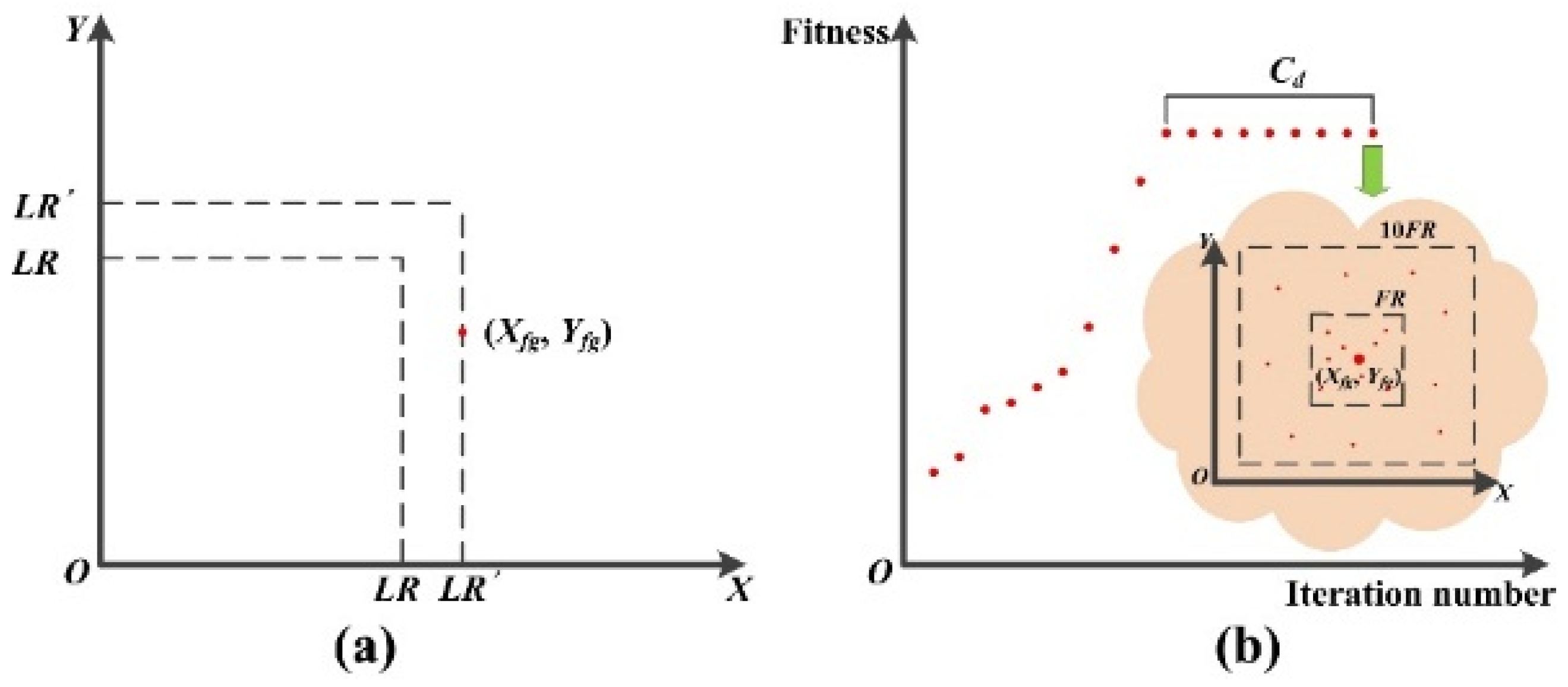
3.1. Improvement on FOA

It can be seen that basic FOA search optimal solution is in the neighborhood of previous group location only. In other words, the location of each fruit fly during the iteration process is determined according to previous swarm coordinate and the preset fly distance range. The optimization is therefore simplified further to shorten the program code and decrease the convergence time. Unfortunately, an excessive pursuit of local searching ability has also reduced the diversity of the fruit fly swarm. The basic FOA can easily to fall into a local extreme due to poor global searching capacity. In order to balance the optimization process, a variation coefficient C_v and a disturbance coefficient C_d are introduced during the process of producing new fruit flies to enhance the group diversity. The principle of the two coefficients is presented in Figure 1.

The smell concentration of each individual is calculated to search the maximal fitness in Step 3.3. Then, the concentrations are ranked as (smell₁, smell₂, smell₃, …, smell_i, …, smell_P), where smell₁ is the biggest and smell_P is the worst. For any smell_i > C_v, the location of the corresponding fruit fly is updated according to Equation (11). That is to say, the fly moves towards the best one. If smell_i < C_v, the variation operation is conducted and the fly obtains its location in a new way, which can be expressed as follows:

$$\{\begin{array}{l}{X}_i=\mathrm{rand}(LR\prime )\\ Y_i=\mathrm{rand}(LR\prime )\end{array}$$

(15)

where LR′ = max(LR, X_fg, Y_fg), the reason lies in the coordinate range of the fruit fly swarm may exceed the original scope with the optimization process. The location of the variation fly is updated in a bigger range randomly to search appropriate solution.

Moreover, the disturbance coefficient C_d is introduced when the position of the group remained unchanged for several iterations. Assuming that the smellbest after m-th iteration could be presented as smellbest_m and smellbest_n for n-th, if smellbest_m = smellbest_n and n − m > C_d, then the location of each fruit fly can be obtained as follows:

$$\{\begin{array}{l}{X}_i=X_{fg}+10\mathrm{rand}(FR)\\ Y_i=Y_{fg}+10\mathrm{rand}(FR)\end{array}$$

(16)

where i = 1, 2, 3, …, P. The aim of the disturbance operation is to expand the searching area when the preset fly distance range does not work in finding a better smell concentration for the fly swarm. The flowchart of the proposed IFOA is shown in Figure 2.

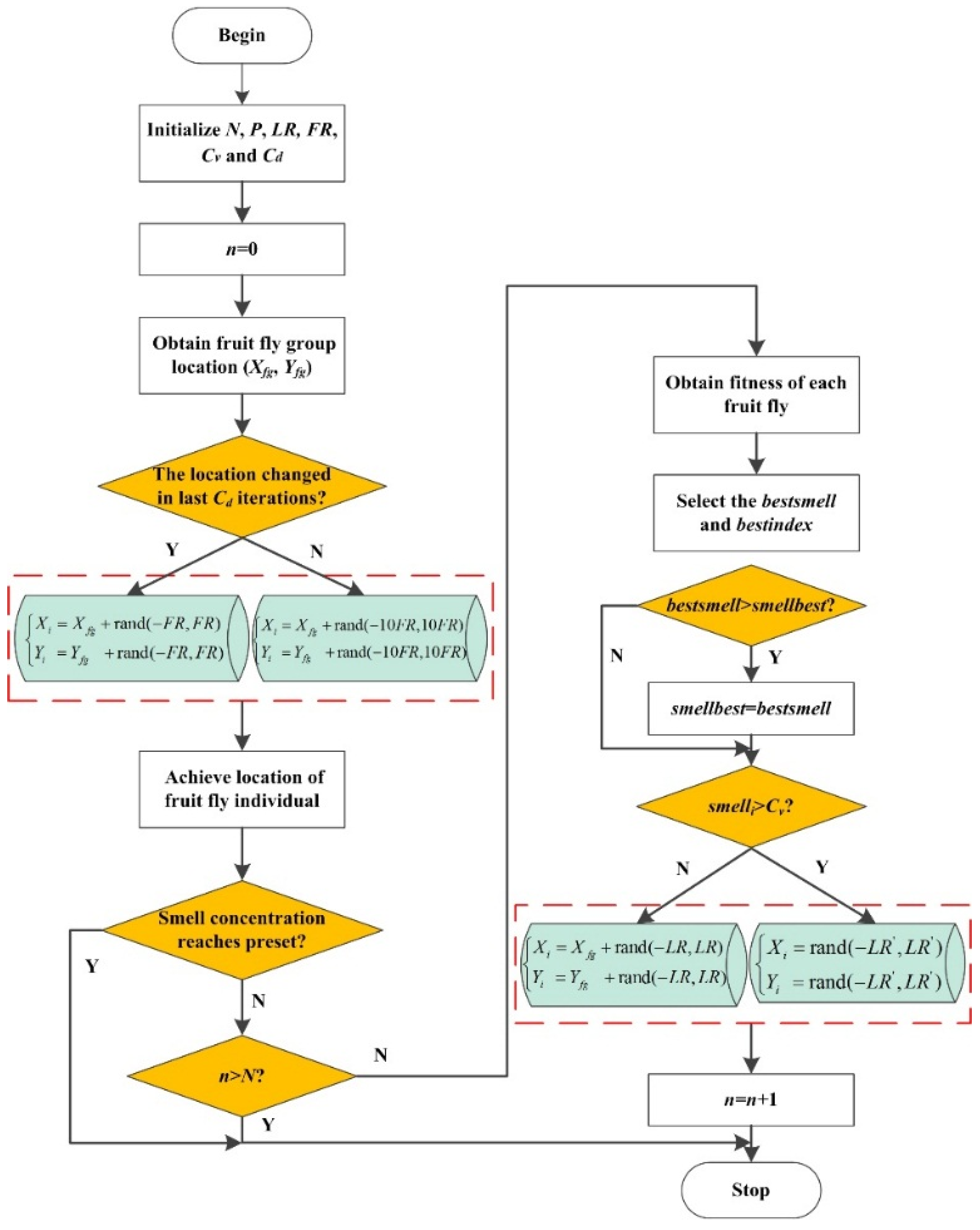
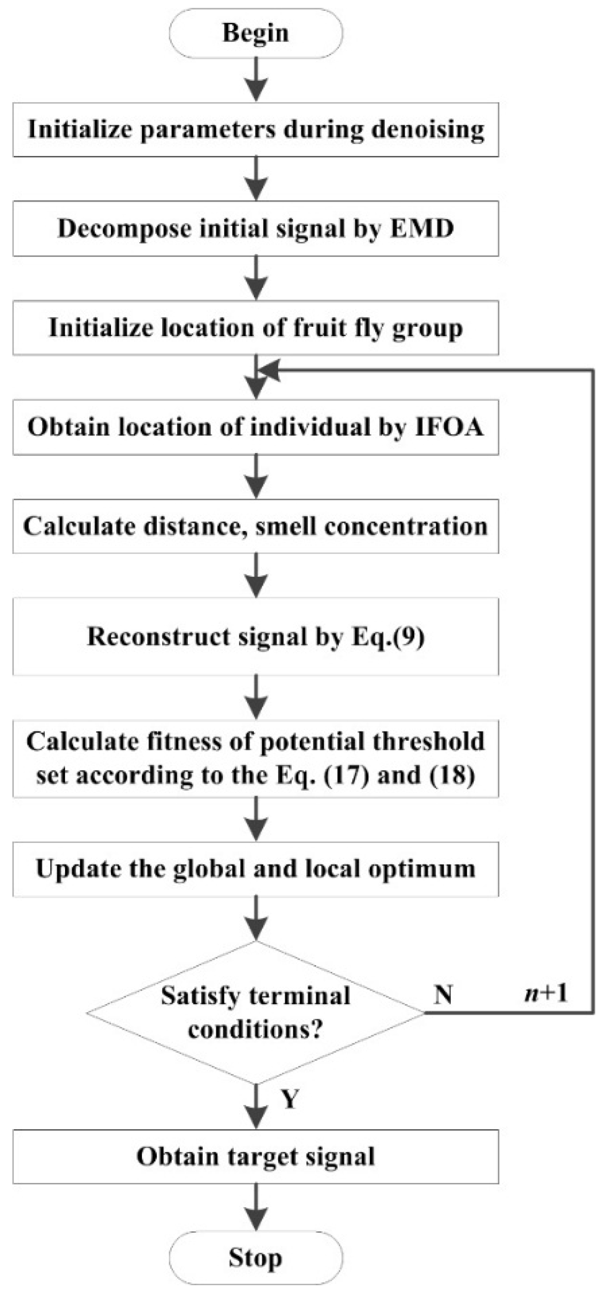
3.2. Flow of the Proposed Denoising Method

In order to eliminate noise component from the acoustic signal adaptively, an EMD-based denoising solution optimized by an improved FOA is proposed in this paper. As some key denoising parameters in Equations (5) and (6), such as C, α and β, are estimated according to statistic and experiment analysis, the determination of denoising threshold is always tough work and consumes much time. Moreover, an appropriate threshold gives significant efficiency of the EMD-based noise elimination process. In order to solve the above problems, the denoising thresholds in Equation (7) or (8) are determined automatically through the improved FOA instead of Equations (5) and (6). The flow of the proposed EMD-IFOA can be summarized as follows:

Step 4.1: Parameter initialization. The parameters in EMD-IFOA such as the lower-order coefficient M₁ and high-order coefficient M₂ are given firstly, so the number of fruit fly group is M₂ − M₁ + 1. The maximal iteration number is N, the number of fruit flies in each swarm is P, the terminal fitness η, the fruit fly location range LR , the random fly distance range is FR, the variation coefficient C_v and disturbance coefficient C_d. The initial locations of the fruit fly groups are obtained by Equation (10).

Step 4.2: Signal decomposition. The original noise-added signal x(t) is decomposed by EMD, which can be presented as x(t) = imf₁ + imf₂ + … + imf_k + res.

Step 4.3: Threshold optimization. The location and smell concentration judgement of each fly individual can be obtained by the improved FOA subsequently. It should be pointed out that any M₂ − M₁ + 1 smell concentration from different fruit fly swarm can be treated as a potential optimal combination of threshold set. For example, S_ij donates i-th smell concentration judgement in j-th swarm, where i = 1, 2, 3, …, P, j = 1, 2, 3, …, M₂ − M₁ + 1. Then, the useful and noise signal are separated by hard threshold function in Equation (7) or soft function in Equation (8). The estimated signal is reconstructed as the final series according to Equation (9). In order to evaluate the denoising performance of different thresholds, a fitness function or smell concentration function in IFOA based on the independent measurement principle is established as follows:

$$f=\frac{1}{1+g}$$

(17)

$$g=\frac{{[r_{22}\times h{r}_{21}]}^2}{{r_{11}}^2}$$

(18)

where r₁₁ and r₂₂ are second-order correlation coefficient of useful signal and noise signal, respectively, and hr₂₁ is high-order correlation coefficient between the two series. An increasing value of r₁₁ implies that the useful component is more than the component of noise. If r₂₂ and hr₂₁ are decreasing, then it means that the two signals become more independent to each other. Thus, the original signal and noise are separated gradually. In general, the noise elimination process performances are better with larger r₁₁ and smaller r₂₂ and hr₂₁.

Step 4.4: Iteration termination. If the iteration number reaches N or the fitness reaches the preset value η, the iteration process is terminated; otherwise, the optimization is continued. The flow of the proposed denoising method based on EMD-IFOA can be presented as Figure 3.

4. Simulation and Analysis

In order to validate the effectiveness and superiority of the proposed method, a piece of simulated train acoustic signal taken from Matlab 2015b Signal Processing Toolbox (8.6, MathWorks Inc., Natick, MD, USA) was extracted as the original pure signal. Then, Gaussian white noise with different signal-to-noise ratio (SNR) was added into the pure signal. Three evaluation parameters were introduced to make a comprehensive comparison amongst wavelet threshold denoising, traditional EMD denoising, EMD-PSO denoising, EMD-FOA denoising and the proposed EMD-IFOA.

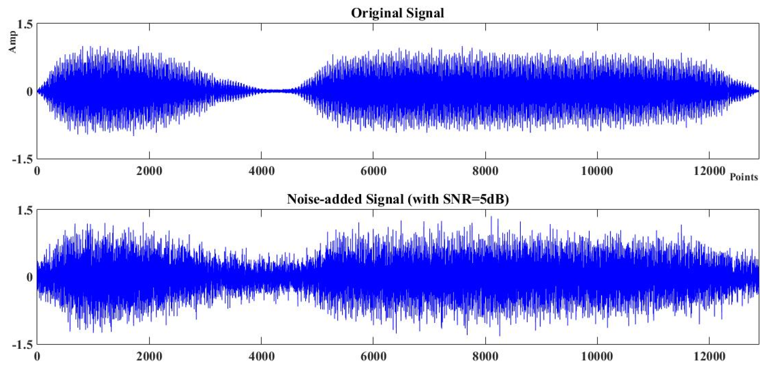
4.1. Signal Preprocessing

To test the performance of the denoising methods, a piece of pure sound signal series was necessary. As machinery sound collected directly from industrial field was always polluted by the environment background noise, the most convenient method to obtain a clean signal was by synthetizing using simulation. In this paper, a piece of simulated train acoustic signal with sampling frequency of 8192 Hz and length of 12,880 taken from Matlab 2015b Signal Processing Toolbox was extracted as the original pure signal y. Then Gaussion white noise n was added into the original signal. The SNR was introduced to measure the content of noise in the noisy signal x, which could be presented as follows:

$$\mathrm{SNR}=10\lg \frac{P_y}{P_n}$$

(19)

where P_y and P_n were effective power of pure signal and noise respectively. The original train sound signal and the noise-added signal with SNR = 5 dB were presented in Figure 4.

4.2. Signal Decomposition and Denoising

Five different denoising solutions with SNR = 5 dB were conducted as follows:

(1)

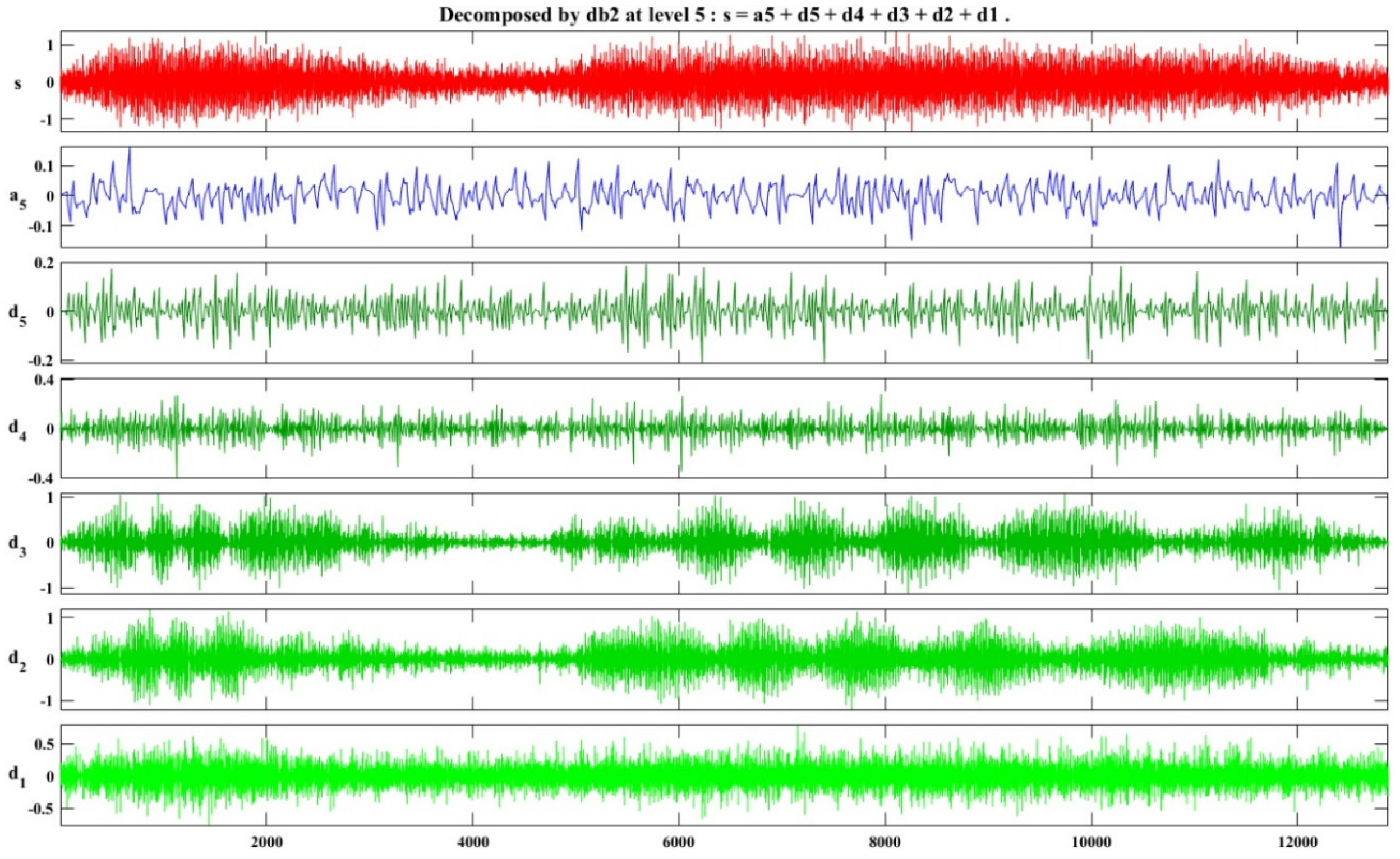
Wavelet threshold denoising. The noisy signal was first decomposed by db2 wavelet at five levels [32], and the decomposition result was presented in Figure 5. Then, the soft threshold function was adopted to shrink the wavelet coefficients. Inverse wavelet transform was conducted consequently to reconstruct the signal.

(2)

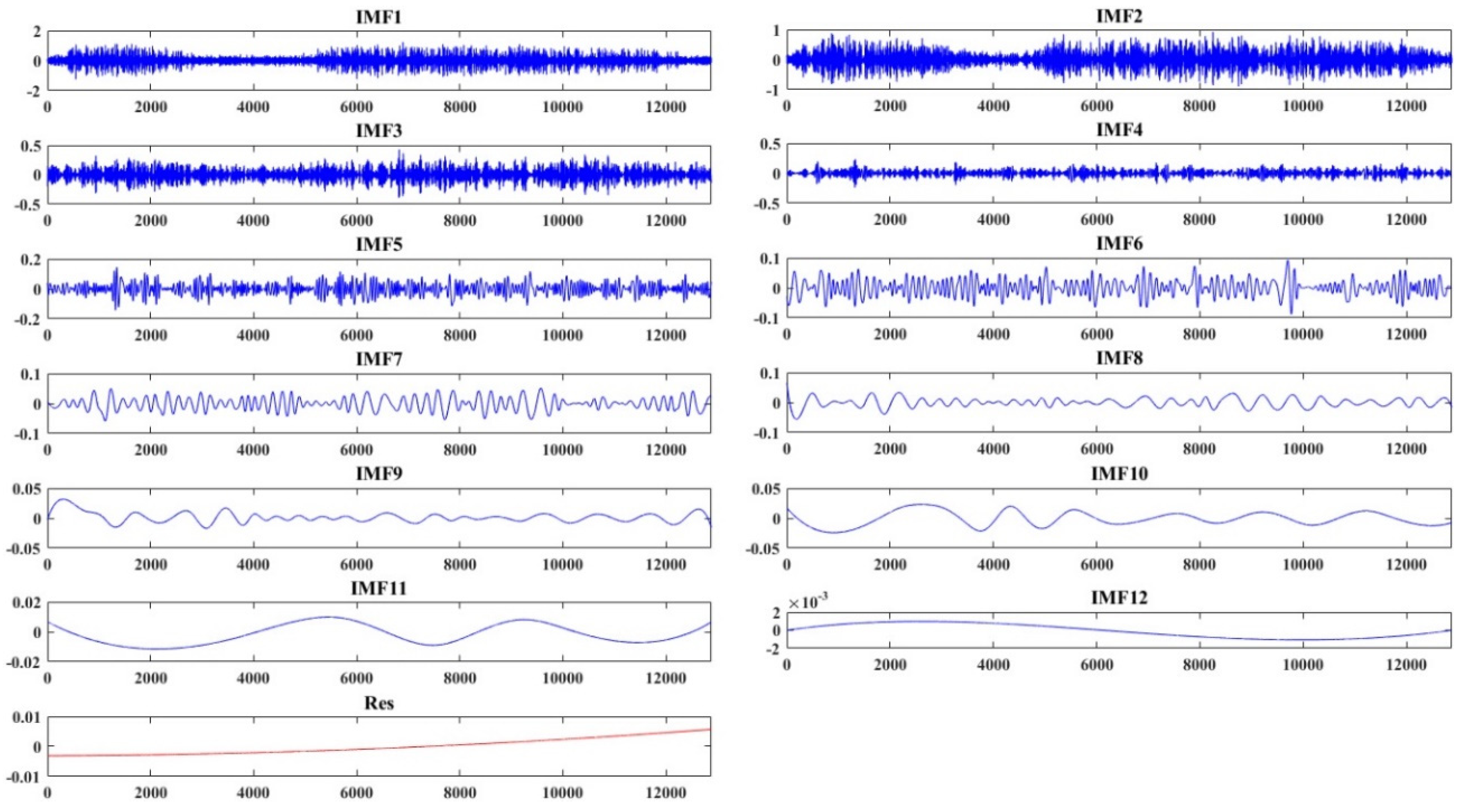
EMD denoising. The noisy signal was first decomposed by EMD adaptively, which could be shown in Figure 6. The noisy signal could be decomposed as x = imf₁ + imf₂ + imf₃ + … + imf₁₂ + res. Then, the shrinkage threshold of each IMF was determined according to Equations (5) and (6). Soft threshold function was applied and the denoised signal was reconstructed as Equation (9). Some parameters in Equations (5), (6) and (9) were set as follows [10]: C = 0.7, α = 0.719, β = 2.01, M₁ = 2 and M₂ = 4.

(3)

EMD-PSO denoising. The noisy signal was first decomposed by EMD adaptively. Then, the threshold of each IMF was determined according to PSO intelligently. Soft threshold function was applied and the denoised signal was reconstructed as Equation (9). Some parameters during the EMD-PSO were set as recommended in [23]: M₁ = 2, M₂ = 4, the dimensionality of each particle was M₂ − M₁ + 1 = 3, the learning factor c₁ and c₂ were set as 2, the iteration number was 100 and the particle number of the population was 10.

(4)

EMD-FOA denoising. The noisy signal was first decomposed by EMD adaptively. Then, the threshold of each IMF was determined according to FOA automatically. Soft threshold function was applied and the denoised signal was reconstructed as Equation (9). Some parameters during the EMD-FOA were set as follows: M₁ = 2, M₂ = 4, the number of fruit fly population was M₂ − M₁ + 1 = 3, the iteration number was 100, the fly number in each population was 10, the fruit fly location range and the random fly distance range was 1.

(5)

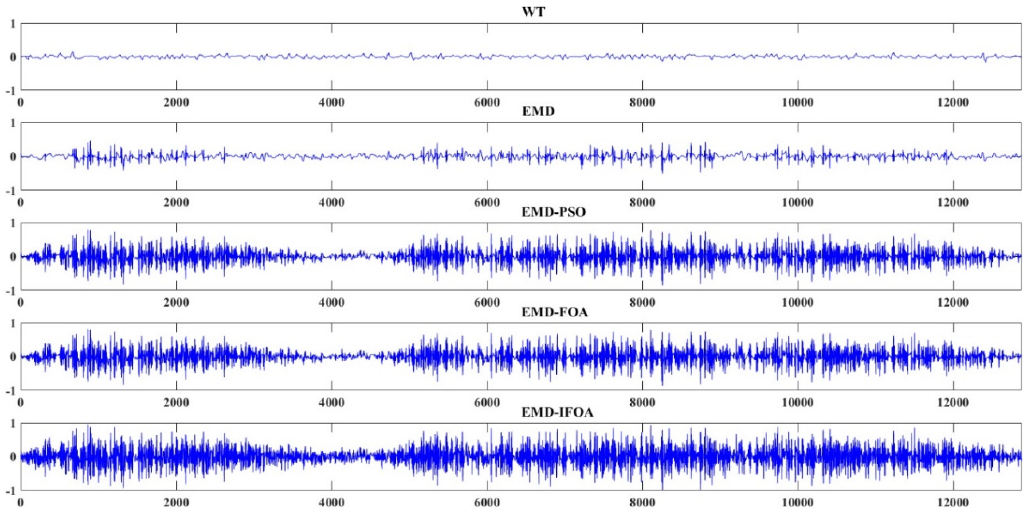
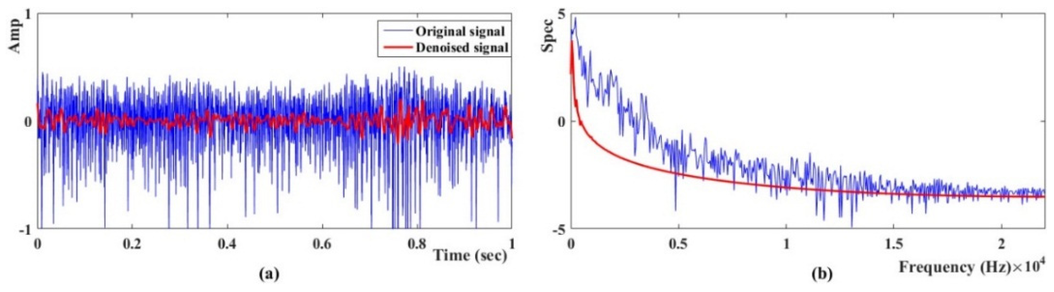
EMD-IFOA denoising. The noisy signal was first decomposed by EMD adaptively. Then, the threshold of each IMF was determined according to IFOA automatically. Soft threshold function was applied and the denoised signal was reconstructed as Equation (9). Some parameters during the EMD-IFOA were set as follows: M₁ = 2, M₂ = 4, the number of fruit fly population was M₂ − M₁ + 1 = 3, the iteration number was 100, the fly number in each population was 10, the fruit fly location range and the random fly distance range was 1, the variation coefficient C_v = 0.2 and disturbance coefficient C_d = 5. The denoised signal of the five noise elimination schemes are presented in Figure 7.

In order to evaluate the noise reduction performance of the five methods, three appraisal parameters such as the mean squared error (MSE), SNR improvement (SNR_imp) and percent root mean square difference (PRD) were adopted and defined as follows:

$$\mathrm{MSE}=\frac{1}{N}{\displaystyle \sum _{i=1}^N{(y_i-{\tilde{x}}_i)}^2}$$

(20)

$${\mathrm{SNR}}_{\mathrm{imp}}=10\lg \left(\frac{{\displaystyle \sum _{i=1}^N{(x_i-y_i)}^2}}{{\displaystyle \sum _{i=1}^N{({\tilde{x}}_i-y_i)}^2}}\right)[\mathrm{dB}]$$

(21)

$$\mathrm{PRD}=\sqrt{\frac{{\displaystyle \sum _{i=1}^N{({\tilde{x}}_i-y_i)}^2}}{{\displaystyle \sum _{i=1}^N{y_i}^2}}}$$

(22)

where y was the original signal, ${\tilde{x}}_i$ was the denoised signal and x was the noise-added signal. The results were shown in

Table 1. The denoising performance of the five methods (with SNR = 5 dB). SNR: signal-to-noise ratio; MSE: mean squared error; PRD: percent root mean square difference; SNR_imp: signal-to-noise ratio improvement; EMD: empirical mode decomposition; PSO: particle swarm optimization algorithm; FOA: fruit fly optimization algorithm; IFOA: improved fruit fly optimization algorithm.

Index	Wavelet	EMD	EMD-PSO	EMD-FOA	EMD-IFOA
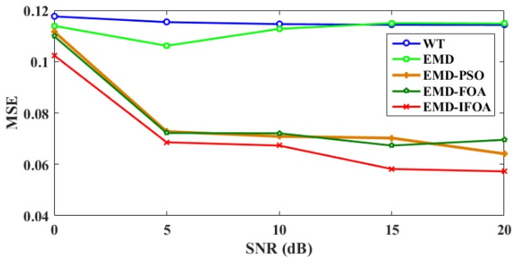
MSE	0.1154	0.1062	0.0728	0.0722	0.0686
SNRimp (dB)	−5.0651	−4.7038	−3.0634	−3.0298	−2.8053
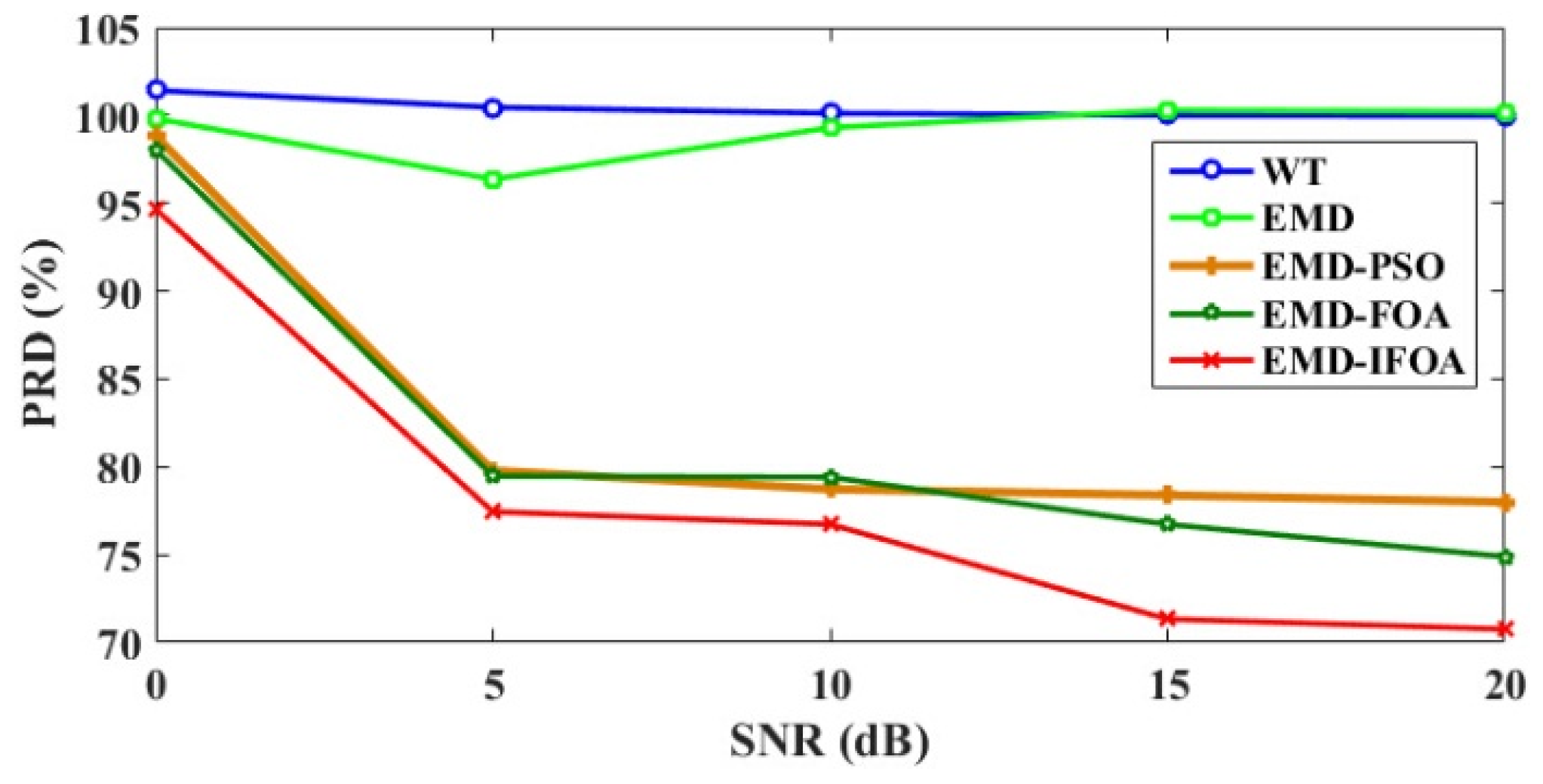
PRD	100.46%	96.36%	79.78%	79.47%	77.44%

.

It can be seen from the Figure 7 and Table 1 that adaptive noise cancellation methods based on intelligent searching technology performed better than wavelet and traditional EMD threshold denoising. The selection of wavelet basis and decomposition level might be inappropriate. The recommended threshold for wavelet and EMD denoising shrank the decomposed coefficients excessively, which resulted in an amplitude of denoised signal that was much smaller compared with the original signal. The EMD-FOA exhibited slightly better than the EMD-PSO. Moreover, the EMD-IFOA had obvious preponderance of the MSE, signal-to-noise ratio improvement (SNR_imr) and PRD compared with the previous four schemes, which indicated that basic FOA and PSO fell into the local extreme during searching optimal threshold and the population diversity of the EMD-IFOA was enhanced to produce more threshold candidates. The MSE of EMD-IFOA decreased 5.77% and 4.99% compared with EMD-PSO and EMD-FOA. The PRD reduced 2.34% and 2.03% respectively. The SNR_imr of the proposed method improved 8.43% and 7.41% compared to the other two intelligent denoising approaches.

In order to research the denoising performance at different SNRs, a further comparison was made and the average value of ten simulation results was discussed. The performance of the proposed and other four denoising methods in 0 dB, 5 dB, 10 dB, 15 dB, 20 dB noisy conditions in terms of MSE is shown in Figure 8. It can be seen from the figure that the MSE did not have an obvious difference when the SNR was greater than 10 dB for wavelet and EMD threshold denoising. The other three denoising approaches based on intelligent optimization solutions outperformed both in higher and lower noise component. As expected, the proposed EMD-IFOA showed the best performance in all noisy conditions and decreased 8.24% and 6.73% compared with EMD-PSO and EMD-FOA even in the worst case scenario, which proved the proposed method had stronger global searching ability. Another comparison illustrated the performance in term of SNR_imr at different SNR value and was presented in Figure 9. It can be seen from the figure that the SNR_imr decreased almost linearly with the SNR. The proposed method obtained the biggest value in all SNRs than other approaches. Moreover, the PRD of the five methods was presented in Figure 10 and exhibited similar changing tendency with MSE. The PRD of the EMD-IFOA deceased 6.77%, 5.17%, 4.18%, and 3.39% respectively, compared with wavelet, EMD, EMD-PSO and EMD-FOA denoising schemes. In summary, the proposed method exhibited obvious superiority in the denoising effect, which revealed its terrific searching ability.

4.3. Application

In order to test practical performance of the proposed automatic noise cancellation method for the machinery acoustic signal based on EMD-IFOA, an acoustic-based diagnosis system was constructed in the fully-mechanized coal mining working face. The shearer is a kind of essential equipment in modern coal mining, and the operating condition diagnosis for the shearer is of great importance. Conventional diagnosis systems are mainly based on the vibration signal [33] and cutting stress signal [34]. Working lives of the vibration sensors and strain gauges are very short due to the harsh working conditions and contact measurement. The coal output is always restricted due to the frequent maintenance. In January 2016, a working state diagnosis system for coal mining shearers was set up in National Coal Mining Equipment Research and Experiment Center at the China Coal Zhangjiakou Coal Mining Machinery Co., Ltd. (Zhangjiakou, China) to identify whether the shearer was cutting coal seam, rock seam or coal seam-gripping rock. The arrangement of the shearer and the cutting sound collection system were presented in Figure 11. An industrial microphone was installed to collect the sound signal. In order to assure the normal use of the collector under the condition of excessive dust and gas, dust-proof and explosion-proof processing satisfying the coal mining requirements was carried out for the microphone.

As there existed a large number of noise signals among the cutting signal, eliminating noise from the field collected sound signal was a crucial step for improving the recognition accuracy. In order to validate the effectiveness and superiority of the proposed denoising method, a piece of acoustic signal with the sampling frequency of 44.1 kHz and the time duration of 1 s was collected and analyzed. As the frequency spectrum was often applied to further state diagnosis, the frequency distribution of the original field signal and denoised signal were also calculated and presented in Figure 12. It could be seen from the figure that the original signal saltated sharply in amplitude due to the random noise element and the denoised signal turned out to be smooth. Moreover, the frequency component of the original sound was presented disorderly in the whole domain, which resulted in difficulty determining the cutting state of the shearer. While it became regular for the processed signal, some wave peaks which reflected the working state of the shearer appeared in the spectrogram, and other areas were relatively stable. Furthermore, a zoom on the range of [0, 2000 Hz] was shown in Figure 13. It can be seen from the figure that the amplitude of the denoised signal fluctuates at 50 Hz, 260 Hz and 480 Hz. The working state of the shearer can be diagnosed according to the corresponding frequency of the fluctuation and the value of the spectrum. The denoised signal was more suitable for further processing.

5. Conclusions

In order to eliminate noise elements from the sound signal for the acoustic-based diagnosis system, an adaptive threshold denoising method-based EMD and an improved FOA was designed in this paper. Improved strategies on the basis of introducing a variation coefficient and a disturbance coefficient into the basic FOA were applied in the noise cancellation process. The modified FOA is introduced into the threshold determination process of the traditional EMD denoising approach to replace the threshold selection based on statistics estimation and numerous trials. The proposed method can represent an important pretreatment on field sound signals for an acoustic-based diagnosis system. To demonstrate the effectiveness and superiority of the launched WTD-IFOA, a series of simulations were conducted and some comparisons were presented. The performance of the proposed and other four denoising methods in 0 dB, 5 dB, 10 dB, 15 dB, and 20 dB noisy conditions were presented. Overall, the EMD-IFOA had the best results in all noisy conditions. The MSE and PRD of the denoised signal decreased 10.01% and 5.17% respectively even in the worst conditions, and the SNR_imp increased from 0.0151 dB to 0.4767 dB compared with traditional EMD solution. The simulations and comparison results proved that the automatic denoising method could effectively eliminate noise and outperform the others. Finally, an industrial application for the shearer in a fully-mechanized coal mining face was performed to validate field effect. In future studies, the authors plan to investigate some improvements in determining the variation coefficient and disturbance coefficient automatically with the proposed approach.

References

- Elforjani, M.; Mba, D.; Muhammad, A.; Sire, A. Condition monitoring of worm gears. Appl. Acoust. 2012, 73, 859–863. [Google Scholar] [CrossRef]
- Ai, C.S.; Sun, Y.J.; He, G.W.; Ze, X.B.; Li, W.; Mao, K. The milling tool wear monitoring using the acoustic spectrum. Int. J. Adv. Manuf. Tech. 2012, 61, 457–463. [Google Scholar] [CrossRef]
- Zhu, D.C.; Feng, Y.P.; Chen, Q.; Cai, J.B. Image recognition technology in rotating machinery fault diagnosis based on artificial immune. Smart Struct. Syst. 2010, 6, 389–403. [Google Scholar] [CrossRef]
- Gravalos, I.; Loutridis, S.; Gialamas, T.; Avgousti, A.; Kateris, D.; Xyradakis, P.; Tsiropoulos, Z. Vibrational behavior of tractor engine hood. In Proceedings of the 5th International Scientific Conference on Trends in Agricultural Engineering (TAE 2013), Prague, Czech Republic, 3–6 September 2013.
- Garcia, M.P.; Gherabi, A.; Arsenault, H.H. Image difference detection under varying illumination based on vector space and correlations. Optik 2012, 123, 665–669. [Google Scholar] [CrossRef]
- Figlus, T.; Gnap, J.; Skrucany, T.; Sarkan, B.; Stoklosa, J. The Use of Denoising and Analysis of the Acoustic Signal Entropy in Diagnosing Engine Valve Clearance. Entropy 2016, 18, 253. [Google Scholar] [CrossRef]
- Hassanpour, H. A time-frequency approach for noise reduction. Digit. Signal Process. 2008, 18, 728–738. [Google Scholar] [CrossRef]
- Nelson, D.J.; Smith, D.C. Adaptive interference removal based on concentration of the STFT. Digit. Signal Process. 2006, 16, 597–606. [Google Scholar] [CrossRef]
- Tokmakci, M.; Erdogan, N. Denoising of arterial and venous Doppler signals using discrete wavelet transform: Effect on clinical parameters. Contemp. Clin. Trials 2009, 30, 192–200. [Google Scholar] [CrossRef] [PubMed]
- Kopsinis, Y.; McLaughlin, S. Development of EMD-Based Denoising Methods Inspired by Wavelet Thresholding. IEEE Trans. Signal Process. 2009, 57, 1351–1362. [Google Scholar] [CrossRef]
- Pinnegar, C.R. A new subclass of complex-valued S-transform windows. Signal Process. 2006, 86, 2051–2055. [Google Scholar] [CrossRef]
- Donoho, D.L. De-Noising by Soft-Thresholding. IEEE Trans. Inf. Theory 1995, 41, 613–627. [Google Scholar] [CrossRef]
- Donoho, D.L.; Johnstone, I.M. Adapting to unknown smoothness via wavelet shrinkage. J. Am. Stat. Assoc. 1995, 90, 1200–1224. [Google Scholar] [CrossRef]
- Huang, N.E.; Shen, Z.; Long, S.R.; Wu, M.C.; Shih, H.H.; Zheng, Q.; Yen, N.; Tung, C.C.; Liu, H.H. The empirical mode decomposition method and the Hilbert spectrum for non-stationary time series analysis. Proc. R. Soc. Lond. A 1998, 454, 903–995. [Google Scholar] [CrossRef]
- Colominas, M.A.; Schlotthauer, G.; Torres, M.E. Improved complete ensemble EMD: A suitable tool for biomedical signal processing. Biomed. Signal Process. Control 2014, 14, 19–29. [Google Scholar] [CrossRef]
- Yu, X.; Ding, E.; Chen, C.; Liu, X.; Li, L. A Novel Characteristic Frequency Bands Extraction Method for Automatic Bearing Fault Diagnosis Based on Hilbert Huang Transform. Sensors 2015, 15, 27869–27893. [Google Scholar] [CrossRef] [PubMed]
- Ahn, J.H.; Kwak, D.H.; Koh, B.H. Fault Detection of a Roller-Bearing System through the EMD of a Wavelet Denoised Signal. Sensors 2014, 14, 15022–15038. [Google Scholar] [CrossRef] [PubMed]
- Chatlani, N.; Soraghan, J.J. EMD-Based Filtering (EMDF) of Low-Frequency Noise for Speech Enhancement. IEEE Trans. Audio Speech Lang. Process. 2012, 20, 1158–1166. [Google Scholar] [CrossRef]
- Li, M.; Jiang, L.H.; Xiong, X.L. A novel EMD selecting thresholding method based on multiple iteration for denoising LIDAR signal. Opt. Rev. 2015, 22, 477–482. [Google Scholar] [CrossRef]
- Gan, Y.; Sui, L.F.; Wu, J.F.; Wang, B.; Zhang, Q.H.; Xiao, G.R. An EMD threshold de-noising method for inertial sensors. Measurement 2014, 49, 34–41. [Google Scholar] [CrossRef]
- Baskar, V.V.; Abhishek, B.; Logashanmugam, E. Comparison of Fourier Bessel (FB) and EMD-FB Based Noise Removal Techniques for Underwater Acoustic Signals. J. Sci. Ind. Res. 2014, 73, 756–762. [Google Scholar]
- Flandrin, P.; Rilling, G.; Goncalves, P. Empirical mode decomposition as a filter bank. IEEE Signal Process. Lett. 2004, 11, 112–114. [Google Scholar] [CrossRef]
- Lakshmikanth, S.; Natraj, K.R.; Rekha, K.R. Novel approach for industrial noise cancellation in speech using ICA-EMD with PSO. Int. J. Signal Process. Image Process. Pattern Recognit. 2014, 7, 345–358. [Google Scholar] [CrossRef]
- Chu, D.L.; He, Q.; Mao, X.H. Rolling bearing fault diagnosis by a novel fruit fly optimization algorithm optimized support vector machine. J. Vibroeng. 2016, 18, 151–164. [Google Scholar]
- Phuong, N.; Kim, J.M. Adaptive ECG denoising using genetic algorithm-based thresholding and ensemble empirical mode decomposition. Inf. Sci. 2016, 373, 499–511. [Google Scholar]
- Pan, W.T. A new Fruit Fly Optimization Algorithm: Taking the financial distress model as an example. Knowl. Based Syst. 2012, 26, 69–74. [Google Scholar] [CrossRef]
- Li, H.Z.; Guo, S.; Li, C.J.; Sun, J.Q. A hybrid annual power load forecasting model based on generalized regression neural network with fruit fly optimization algorithm. Knowl. Based Syst. 2013, 37, 378–387. [Google Scholar] [CrossRef]
- Zheng, X.L.; Wang, L. A two-stage adaptive fruit fly optimization algorithm for unrelated parallel machine scheduling problem with additional resource constraints. Expert Syst. Appl. 2016, 65, 28–39. [Google Scholar] [CrossRef]
- Xu, J.; Wang, Z.B.; Wang, J.B.; Tan, C.; Zhang, L.; Liu, X.H. Acoustic-Based Cutting Pattern Recognition for Shearer through Fuzzy C-Means and a Hybrid Optimization Algorithm. Appl. Sci. Basel 2016, 6, 294. [Google Scholar] [CrossRef]
- Shan, D.; Cao, G.H.; Dong, H.J. LGMS-FOA: An improved fruit fly optimization algorithm for solving optimization problems. Math. Probl. Eng. 2013, 2013, 108768. [Google Scholar] [CrossRef]
- Li, T.F.; Gao, L.; Li, P.G.; Pan, Q.K. An ensemble fruit fly optimization algorithm for solving range image registration to improve quality inspection of free-form surface parts. Inf. Sci. 2016, 367, 953–974. [Google Scholar] [CrossRef]
- Abbasiona, S.; Rafsanjania, A.; Farshidianfarb, A.; Iranic, N. Rolling element bearings multi-fault classification based on the wavelet denoising and support vector machine. Mech. Syst. Signal Process. 2007, 21, 2933–2945. [Google Scholar] [CrossRef]
- Wang, B.P.; Wang, Z.C.; Zhang, W.Z. Coal-rock interface recognition method based on EMD and neural network. J. Vib. Meas. Diagn. 2012, 32, 586–590. [Google Scholar] [CrossRef] [PubMed]
- Wang, D.; Chen, Y.K. Study on the coal-rock interface identification based on the signal analysis. Min. Process. Equip. 2010, 5, 22–25. [Google Scholar]