Full-Field Optical Coherence Tomography as a Diagnosis Tool: Recent Progress with Multimodal Imaging

Abstract

Full-field optical coherence tomography (FF-OCT) is a variant of OCT that is able to register 2D en face views of scattering samples at a given depth. Thanks to its superior resolution, it can quickly reveal information similar to histology without the need to physically section the sample. Sensitivity and specificity levels of diagnosis performed with FF-OCT are 80% to 95% of the equivalent histological diagnosis performances and could therefore benefit from improvement. Therefore, multimodal systems have been designed to increase the diagnostic performance of FF-OCT. In this paper, we will discuss which contrasts can be measured with such multimodal systems in the context of ex vivo biological tissue examination. We will particularly emphasize three multimodal combinations to measure the tissue mechanics, dynamics, and molecular content respectively.

1. Introduction

Over the past 25 years, optical coherence tomography (OCT) has rapidly developed and spread into many fields of biomedical research thanks to its ability to capture label-free structural contrast deep inside a tissue [1]. Over the years, OCT has been developed into numerous different modalities that emphasize the 3D interplay between tissue microstructures and various specific complementary contrasts [2,3,4,5].

Full-field optical coherence tomography (FF-OCT) is a less familiar OCT-derived technology [6,7]. FF-OCT differs from standard OCT by acquiring 2D en face images in a widefield configuration at a given depth in a tissue. To record a 3D tomogram, the sample is further scanned in depth, instead of acquiring series of A lines as in regular OCT. Such a configuration offers the possibility to use high numerical aperture (NA) microscope objectives, without limiting the exploration depth, and can therefore access submicrometric and subcellular resolution.

FF-OCT has been successfully applied for non-invasive label-free ex vivo pathology assessment in various tissues [8,9,10,11,12,13,14,15]. Thanks to its isotropic micrometric resolution, FF-OCT can often be compared to histology slices. In contrast to histology, FF-OCT does not require time for sample fixation, slicing, or labeling, and an histology-like image can be produced within a few minutes after tissue extraction. It also helps to reduce fixation and slicing artifacts, as FF-OCT does not necessarily require physical slicing, and can image in depth, eventually far from the incision edges for a biopsy.

However, FF-OCT may suffer from its lack of specificity, and sometimes fails to equal the diagnostic capacity of gold standard histology. Yet, FF-OCT detection scores are above 80% for most pathologies in both sensitivity and specificity [14,16], and Manu Jain and colleagues could even report a 100% correct identification of tumors in ex vivo kidneys [17], obtaining similar results to histology, even though the tumor subtyping is still not 100%. In order to increase diagnosis scores, FF-OCT has therefore expanded to multimodal systems combining FF-OCT structural contrast with other pathology biomarkers inside a single microscope. The interest of such multimodal systems is to reduce the ambiguity in structure identification that can arise from sequential imaging with two different microscopes, and to reduce operation time. Some FF-OCT multimodal systems have been reviewed in the recently published Handbook of Full-Field Optical Coherence Microscopy, edited by Arnaud Dubois [16]. We can non-exhaustively mention the multimodal combinations of FF-OCT with fluorescence [18], photothermal imaging [19], elastography [20], polarization [21], multispectral and hyperspectral imaging [22,23,24]. Most of these multimodal systems have been inspired by similar systems developed in standard OCT, but they needed to be adapted and redesigned to fit FF-OCT’s particular configuration.

In this paper, our goal was not to exhaustively describe these multimodal systems, or to systematically review all the potential fields in which multimodal FF-OCT systems can be of interest. Instead, we will start from the need to increase the FF-OCT’s diagnostic ability up to equal that of gold standard histology to describe three different multimodal systems that we are currently developing or improving in our lab. After a brief description of FF-OCT, and the optical systems that we commonly use, we describe and emphasize the differences between FF-OCT and histology contrasts, to better apprehend what contrasts would be optimal to add to FF-OCT. Then, we will describe our recent development related to multimodal systems combining FF-OCT with elastography, with cellular metabolism, and with fluorescence, and how these multimodal systems could increase the diagnosis performance of FF-OCT.

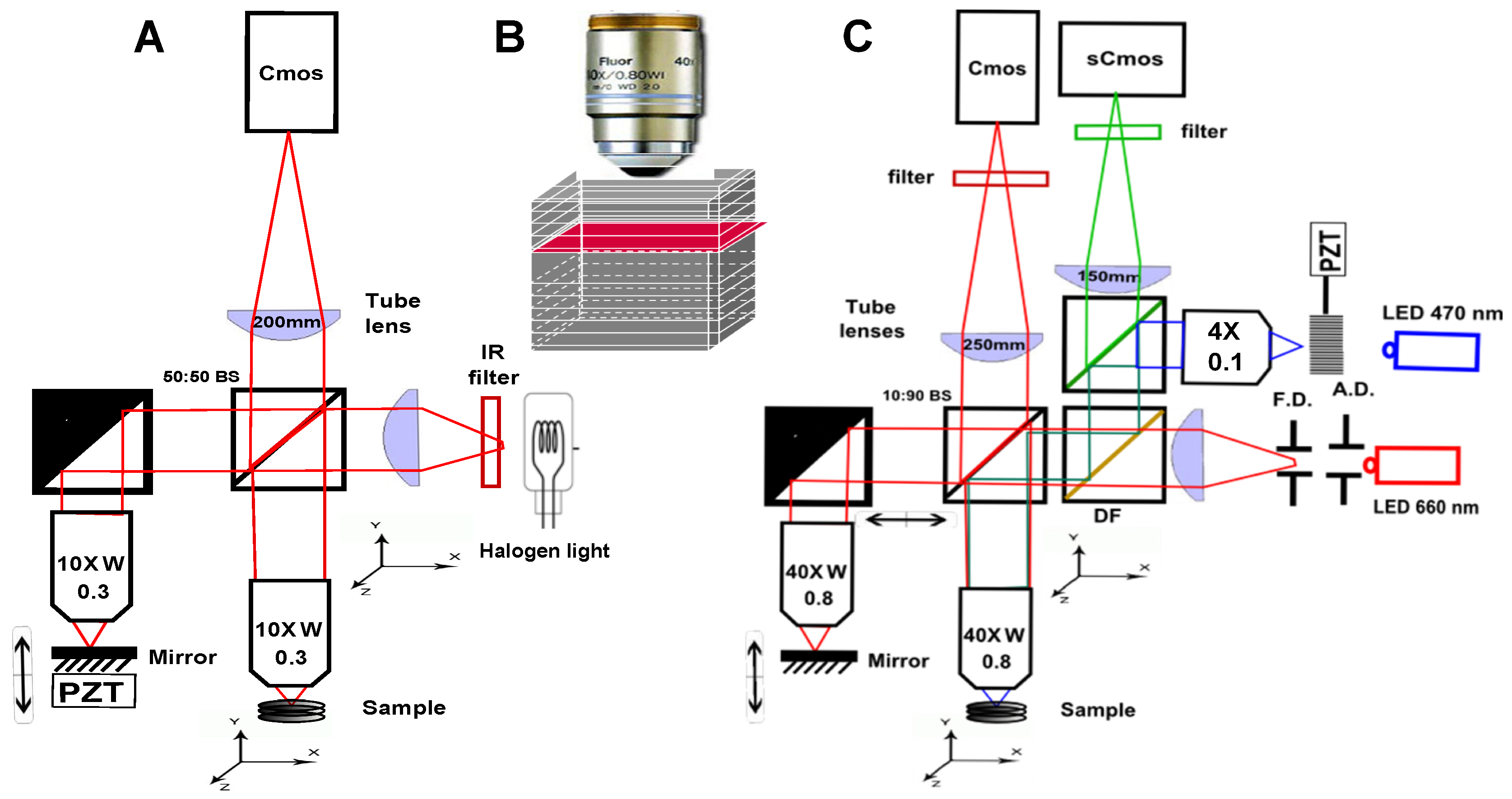
2. Scanning OCT versus Full-Field OCT and Technological Description of the Setups Description

The main difference between classical OCT systems and FF-OCT lies in the absence of transverse scanning. In OCT, or in optical coherence microscopy (OCM), an axial line (A-line) is captured with a single point [1,25,26] or with a line detection [27,28], and further scanned in the transverse plane, to successively obtain 2D planes (B-scan) and 3D tomograms (C-scan). On the contrary, the full-field configuration captures a 2D image at a single depth with a 2D camera, and an axial scan enables the recording of a 3D tomogram. In both configurations, the optical section is mostly controlled by the temporal coherence length, given by the inverse of the spectral bandwidth. Scanning in one dimension compared to two dimensions has several major consequences:

• Because it looks at a single depth at a time, FF-OCT can be performed with a small depth of field, and therefore with high numerical aperture (NA) objectives. This enables high transverse resolution to be obtained, below 1 $\mathsf{\mu }$m for visible light. Other elegant OCT systems have greatly increased their transverse resolution [1,29,30,31,32], however these techniques remain more complex and often have to sacrifice their temporal resolution.
• Moreover, scanning in two directions imposes a trade-off between exposure time and the field of view. In scanning OCT, each pixel is only illuminated for a few microseconds, while in FF-OCT, the entire field of view is usually evenly illuminated during a few milliseconds. It can make a difference in the light dose delivered to the sample, and the most rapid speckle fluctuations are often averaged out [33].
• The time required to get information from the sample is much longer in FF-OCT, since it is limited by the camera frame rate, which is hardly below 1 ms, while some scanning OCT systems can now acquire lines at more than 100,000 lines per second [34]. The consequence is that FF-OCT is much more sensitive to sample motion, and is difficult to perform in vivo, other than on anesthetized animal or by pressing the sample against an imaging window [35].
• A last important difference when looking at en face images either performed in scanning OCT or FF-OCT is that all the pixels have been acquired at different times in OCT, while they are acquired at the same time in FF-OCT (if the camera is operated in global shutter mode), which can introduce some artifacts when looking at moving objects. On the other hand, all axial pixels are acquired simultaneously in OCT, while they are largely separated in time for FF-OCT. An important consequence is that the optical phase can be directly retrieved in OCT by subtracting two adjacent axial pixels [36] while FF-OCT requires multiple phase-shifted measurements to retrieve the optical phase.

In practice, we mainly use two different FF-OCT layouts presented in Figure 1. The first setup is the LLTech commercial system [37], based on a Linnik interferometer using two identical 10X, 0.3 NA microscope objectives, and a thermal source to produce an isotropic resolution of 1 $\mathsf{\mu }$m. We also developed custom-built versions of this system, exhibiting higher mechanical stability, or different cameras for example, but the general layout stays identical. We used these systems to add elastography [20,38] and motility contrasts [39,40].

The second setup is a multimodal setup combining FF-OCT and structured illumination fluorescence microscopy (SIM) [41], in a relatively similar layout to the one developed by H.Makhlouf and colleagues [42]. To enhance the photon collection, we used higher NA objectives, either 40X, 0.8 NA in water, or 30X, 1.05 NA in silicone oil, achieving transverse resolution below 500 nm, and depth of focus between 1 and 2 $\mathsf{\mu }$m. Interestingly, in this system, the optical sectioning ability comes from the lateral spatial coherence [43,44] controlled by the depth of focus, and therefore the objective NA rather than the temporal coherence, meaning that simple LEDs can be used without sacrificing the axial resolution. Both systems are illuminated by spatially incoherent sources, which eliminate the cross talks [45], and preserve the transverse resolution from degradation due to low order aberrations [46]. The illumination sources are mounted in a Kohler illumination to provide an illumination as homogeneous as possible.

Both systems are now operated with a new CMOS camera developed by Adimec during an ERC project (CAReIOCA) led by LLTech [47]. This camera can handle a Full Well Capacity of about 2Me${}^{-}$ on 2 million pixels at frame rates up to 700 Hz, which typically enhanced our signal-to-noise ratio by a three-fold factor, and acquisition speed by a five-fold factor, with respect to previously used cameras (PhotonFocus, MV1-D1024E-160CL, Lachen, Switzerland).

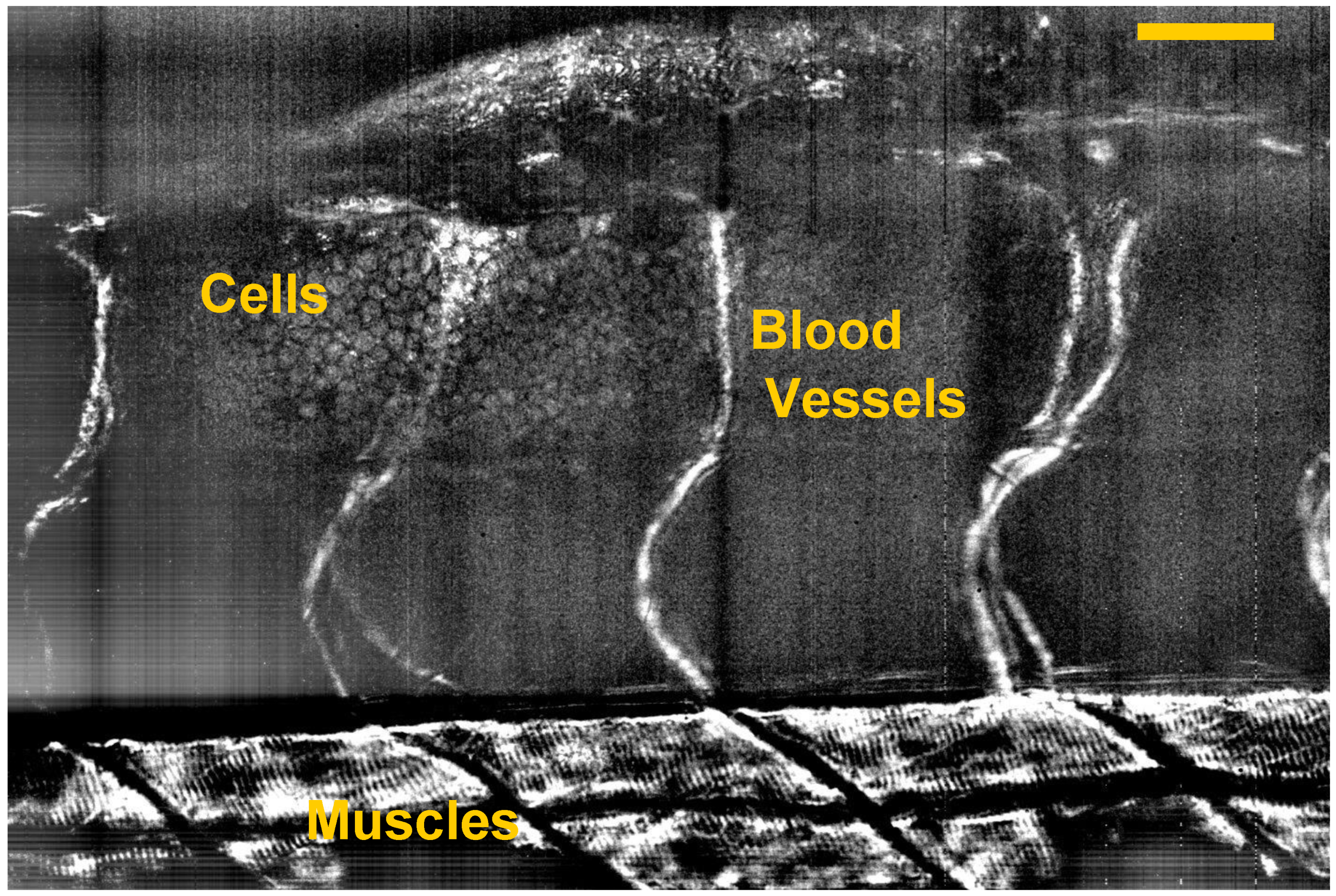
3. FF-OCT and Histology Contrasts

In order to further compare histology and FF-OCT, we describe in this section histology contrast and procedures.

It is commonly said that Marcello Malpighi is the precursor of modern histology, as he was the first scientist to carefully describe micro-anatomic features of plants and animal tissues by the end of the 17th century with the first microscopes [48,49]. Since then, histology has continuously benefited from advances in chemical labeling and fixatives, and has benefited from a better understanding of tissue nanostructures and organization thanks to electron microscopy [50]. It now benefits from an extensive literature, and from digital atlases [51,52,53] enabling direct comparisons with normal or pathological slices of most tissues. However, the basic microscopy principles have mainly remained unchanged since the beginning of histology. They consist of imaging a thin slice of a sample with a simple transmission optical microscope. Since light absorption and scattering by biological structures exhibit a low contrast, histology commonly uses chemical agents to reveal specific contrasts of interest [54,55,56]. The most common staining uses two associated stains, Hematoxylin and Eosin (H & E), that respectively label chromatin and chromosomes in blue, and cytoplasm in red. Hemoglobin usually appears orange, and collagen fibers appear pink. This staining is particularly versatile, as it can be used with a variety of fixatives. A wide range of different staining can be applied to a tissue slice. We can non-exhaustively evoke Golgi staining that labels 1% to 2% of neurons with silver that absorbs light to appear dark, Nissl staining that labels nucleic acids, or tetraoxide osmium that labels unsaturated lipids and lipoproteins. If many subcellular structures can be selectively labeled, it is often difficult to combine different stains in a single slide. However, using specific labels imposes a prior knowledge of the tissue composition, and of the pathology, and some unlabeled biomarkers could be missed.

Moreover, histology requires tissue fixation, performed either chemically or by freezing the sample, and physical slicing of the tissue, usually performed by a microtome. The fixation first goal is to harden the sample to be able to cut it in thin sections. However, fixation can introduce strong artifacts, as it often removes lipidic structures, and can increase the tissue volume. The physical slicing can induce physical damage, notably in neuronal tissues, in which many axial neurites are usually cut, leading to neuronal death. Finally, these two steps are usually time consuming, and can lead to the physical destruction of the samples if not adequately performed.

In the case of histopathology, the tissue is often fixated by replacing water by paraffin, and is then sliced in 4 to 5 $\mathsf{\mu }$m slices. For each slice, the dyes have then to diffuse through the paraffin scaffold. In total, these processes can last for a few days.

In the case of intra-operative histology, the time allowed to the pathologist is usually not more than 15 to 30 min. To meet these time requirements, the sample is frozen, and directly sectioned and colored. However, many tissues, such as fat, brain, or retina, are not well suited for this process, and the number of available labeling is limited.

On the other hand, OCT was only invented 25 years ago, and its full-field version is 18 years old, so comparatively little literature and atlases can be found [57]. However, OCT and FF-OCT provide a label-free, and optically-sectioned imaging. This means that imaging can be performed right after tissue extraction, which can provide a very fast diagnosis, and could even ideally provide an intra-operative diagnosis to efficiently define a tumor margin for example.

The main advantage of OCT is its virtual sectioning ability, enabling imaging at a few hundred microns below the tissue surface, hence reasonably far from the sectioned surface no matter which section is required [58]. To completely remove slicing artifacts and reach large depths, OCT systems have successfully been coupled to a vibratome, in a procedure where an entire volume is imaged before a physical slice smaller than the imaged volume is performed [59].

Additionally, OCT systems capture the light naturally backscattered by the sample, without using any label. Working label-free can be advantageous, as staining artifacts can be avoided, and as it can importantly reduce the time prior to imaging. On the other hand, the recorded signal often lacks specificity. The obtained contrast is complicated to predict, as it is described by multi-scale complex theories, notably combining Rayleigh and Mie theories, depending on the scatterer size [60]. However, for a given tissue, the obtained contrast is highly reproducible, so the diagnosis performance could be increased only by simply better characterizing the typical contrast obtained on each tissue, and each condition.

Quite generally, we can nevertheless emphasize the strong ability of FF-OCT to detect high refractive index (high lipid or high fat content) fibers, such as collagen fibers [8], myelin fibers [61], and even some large unmyelinated axons in the eye [62]. Moreover, in terms of contrast, looking at the backscattered light can differ substantially from transmission microscopes in thick samples. However, one can assume that for thin slices, the contrast in reflection is mainly the inverted contrast for scattering structures and the same contrast from absorbing structures compared to a transmission microscope.

The label-free ability of OCT has a final practical advantage, since the imaging can be performed prior to any tissue modification. It means that the same tissue can be further used for another procedure, including a standard histology procedure [8], or fluorescence labeling. It is usually preferred to perform the OCT imaging before any sample modification, as OCT signal alteration can occur after fixation, depending on the tissue content [62] (especially since fixatives often remove lipidic structures of the cells). Keeping this in mind, it is nevertheless possible to perform histology-like measurements in fixed tissues [58].

Scanning OCT has also been used successfully to perform histology-like measurements [58,63,64,65], and to detect tumor regions [66,67] through changes in the collagen content [68], the tissue microangiogram and backscattering [69], or in the tissue fractal dimension [70]. However, we believe that the high resolution of FF-OCT can significantly improve the diagnostic abilities of OCT [8,17]. With higher numerical apertures, the light collection is improved which helps to reveal more structures and increase the signal-to-noise ratio for the calculation of backscaterring coefficients or fractal dimensions [40,71]. Signal from cell contours and from intracellular structures can also be detected. This will be described in Section 5 on Dynamic FF-OCT. Finally, the en face view of the sample is quite natural for histologists, as it looks similar to histology slides. FF-OCT is also faster than scanning OCT to record a single en face image.

Figure 2 shows a comparison between FF-OCT and a regular H & E histology in a breast sample, the organization of which is altered by a ductal carcinoma in situ (DCIS). FF-OCT notably reveals normal adipocytes, normal and abnormal collagen fibers (based on their scattering strength), and enlarged ducts. These indicators are characteristics of DCIS, that could be identified with 90% sensitivity and 75 % specificity in this case [14].

4. FF-OCT and Biomechanics

Since the early beginning of medicine, palpation has been used to qualitatively assess abnormal tissue stiffness associated with several diseases. Palpation-based diagnosis of heart, abdomen, and wounds diseases or infections has been reported in many ancient cultures, such as Greek, Egyptian, or Chinese medicine [72,73]. The mechanical properties of tissues and cells are mostly related to their structure and function, and changes in a tissue’s biomechanical properties can reveal its pathological state [74]. Notably, biomechanical changes can include the stiffness increase due to an extracellular matrix accumulation, including collagen accumulation, associated with liver fibrosis, and ultimately cirrhosis [75,76]. Moreover, tumor development significantly and progressively impacts the tissue biomechanics [77]. More importantly, the tumor stiffness actively increases its progression, and thus its malignancy, partly through a mechanically-induced molecular circuit, leading to the reduction in the number of tumor suppressors [78]. Therefore, not only tissue stiffness, but also stiffness anisotropy can be used as relevant diagnosis parameters.

In the 1980s, the thorough and quantitative measurement of tissue elasticity was developed, giving access to stiffness in the approximation of purely elastic deformation of tissues. Elastography has been introduced in biomedical imaging with ultrasound and MRI elastography [79,80], and has been proven to be a precious diagnosis biomarker for physicians since then [81,82]. In this paper, we will only discuss tissue biomechanics in comparison to palpation-based diagnosis, and therefore at macroscopic and mesoscopic scales. However, we can add that cellular and molecular biomechanics can also be significant biomarkers of diseases, but they stay difficult to measure in tissues. To our knowledge, the most promising technique to study microscopic biomechanics inside a tissue is fluorescent FRET sensors [83].

In OCT, mechanical contrast has been introduced by Schmitt in 1998 [84]. Since this pioneering work, many methods have been developed with success such as 2D, 3D, static or dynamic elastography [84,85,86,87,88]. In FF-OCT, our group adapted two similar approaches to measure mechanical contrast. The first approach is a static method based on a finite element 3D correlation algorithm that gives access to the 3D local strain tensor inside the samples [20], giving access to the local shear modulus, which is itself proportional to the tissue elasticity, or stiffness for soft tissues. The second approach is a quantitative dynamic method based on shear wave speed imaging, inspired by similar experiments performed in ultrasounds developed in our lab. Using a fast FF-OCT system working at up to 30,000 frames per second, we could measure the local shear wave speed which is directly related to the local shear modulus [38].

In this section, we present a brief description of both methods and some results obtained on biological samples.

4.1. Description of the Different Mechanical Parameters and Approximations

Before describing how it is possible to optically measure tissue biomechanics, we briefly summarize here the numerous different mechanical parameters that can be found in the extensive literature on tissue biomechanics. We will emphasize the relationship between these parameters, and their relevance for diagnosis.

Most studies in MRI, as well as in ultrasound or optics, focus on the elastic properties of tissues, meaning the reversible linear deformation $\overline{\overline{\epsilon }}$ caused by a small mechanical stress $\overline{\overline{\sigma }}$. In the elastic regime, and neglecting viscosity, the generalized Hooke’s law gives:

$$\overline{\overline{\sigma }}=\overline{\overline{\overline{\overline{C}}}}.\overline{\overline{\epsilon }}$$

(1)

where $\overline{\overline{\overline{\overline{C}}}}$ is a fourth order tensor, named stiffness tensor, that depends on the mechanical parameters of the sample. All the other parameters that we will describe are elements of this fourth order tensor, and are usually obtained when the dimensions of the generalized problem are reduced. For example, Young’s modulus E corresponds to the linear coefficient that relates a purely axial stress, and its associated deformation along the stress axis. In this case, the problem is reduced to a single dimension:

$$\mathrm{E}=\frac{\epsilon }{\sigma }$$

(2)

We can add that Young’s modulus is qualitatively the main measurement that is performed with manual palpation. Basically, the first information that one can get with manual palpation is how the tissue resists to an axial deformation or stress, which is given by the Young’s modulus.

From Equation (1), it is easy to realize that a given sample is not only deformed in the direction of the stress, but can also be deformed in the transverse direction, with a preferential axis for anisotropic material. We will describe in Section 4.2 an example metric to quantify the local anisotropy of a sample.

In addition to these parameters, many mechanical measurements rely on shear wave speed measurement that we will describe more carefully in Section 4.3. The mechanical parameters on which the propagation of mechanical waves depend are simply defined as a result of the wave equation in a medium of a given stiffness. Inside biological media, two waves can propagate [89]: A longitudinal wave that corresponds to compression and traction of the medium with a mechanical displacement parallel to the direction of propagation. Additionally, shear waves can propagate, which correspond to perpendicular mechanical displacements with respect to the direction of propagation. The two waves propagate at speeds c${}_L$ and c${}_{shear}$ respectively that are controlled by the mechanical parameters of the medium. We can therefore define the bulk modulus K, and the shear modulus $\mathsf{\mu }$ with:

$${\mathrm{c}}_L=\sqrt{\frac{\mathrm{K}}{\rho }}$$

(3)

$${\mathrm{c}}_{shear}=\sqrt{\frac{\mathsf{\mu }}{\rho }}$$

(4)

where ρ is the medium local density. These parameters are related to Young’s modulus [89]:

$$\mathrm{E}=\mathsf{\mu }\frac{3K}{K+\frac{1}{3}.\mathsf{\mu }}$$

(5)

Finally, for soft tissues, which represent most biological tissues, except bones, the bulk modulus is much larger than the shear modulus. Bulk moduli of biological samples range from 1 GPa to 10 GPa, while shear moduli range from 0.1 kPa in the brain to 0.1 GPa in epidermis and cartilage, and up to 10 GPa in bones [90]. When considering Equation (5) for soft tissues, the Young’s modulus becomes dependent on the shear modulus only:

$$\mathrm{E}\simeq 3.\mathsf{\mu }\simeq 3\rho {\mathrm{c}}_{shear}^2$$

(6)

With such approximations, we have shown that it was possible to locally measure the Young’s modulus by measuring the propagation speed of shear waves.

4.2. Static Elastography Based on Digital Volume Correlation (DVC)

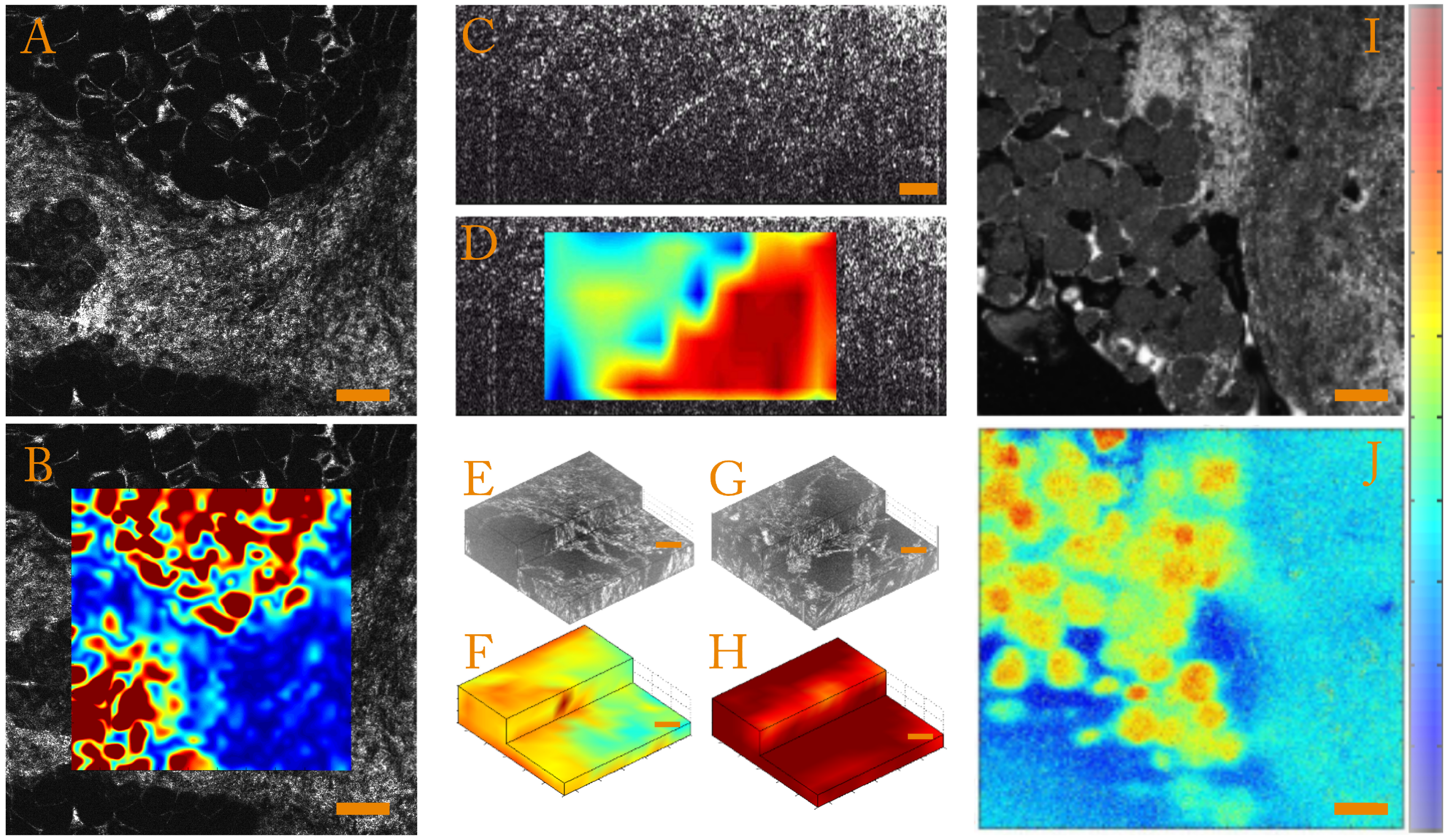
The principle of the static approach is to register a volumetric image before and after mechanical solicitation of the sample [20]. From these two sets of images, we can estimate the 3D local displacement field, $\overrightarrow{u}$, inside the sample using a finite element 3D digital image correlation algorithm developed by S. Roux and his team [91,92]. From the optically measured 3D displacement field, we can calculate the 3D strain tensor $\overline{\overline{\epsilon }}$:

$$\overline{\overline{\epsilon }}=\frac{1}{2}(\overrightarrow{grad}\left(\overrightarrow{u}\right)+{}^t\overrightarrow{grad}\left(\overrightarrow{u}\right))$$

(7)

However, biological samples can be very complex and mechanically heterogeneous. This complexity usually prevents direct access to the local stress tensor and so, in most cases, methods based on digital image correlation are limited to strain contrast and do not provide quantitative stiffness information. This is the main limitation of this type of approach but already the strain information recreates a sort of “virtual local palpation” that can highlight mechanical heterogeneity at the micrometer scale given by FF-OCT or OCT . From the local strain tensor, it is possible to extract different parameters that give access to mechanical information such as strain magnitude or strain anisotropy.

• Strain magnitude
  In order to quantify the strain magnitude, we chose to use an equivalent Von Mises strain defined as:

  $$\forall \overrightarrow{x},{\epsilon }_{eq}\left(\overrightarrow{x}\right)=\sqrt{\frac{2}{3}tr\left(\overline{\overline{\epsilon }}{\left(\overrightarrow{x}\right)}^2\right)}$$

  (8)

  This parameter is independent of the base in which the strain tensor is expressed and allows quantification of the strain amplitude in the case of incompressible media such as biological samples. To illustrate this, we present strain amplitude maps calculated for a human breast tissue in Figure 3A,B, which highlight mechanical differences.
• Strain anisotropy
  The full 3D strain tensor also allows calculation of eigenvalues and eigenvectors of the strain tensor that gives access to information on the mechanical anisotropy of the sample. One should keep in mind that, since the compression of the sample is generally performed along the optical axis, the local stress field is inherently anisotropic. In order to display and to quantify strain anisotropy, we mainly use two parameters. The first parameter is the principal strain direction. For each pixel, the eigenvector corresponding to the largest eigenvalue of the strain tensor is calculated. This vector gives the principal strain direction. For example, Figure 3C is a cross-sectional slice from the volumetric FF-OCT image of a rat heart. In the FF-OCT image, it is difficult to evaluate the fiber direction, and the two different fiber orientations are not visible. However, if the projection angle of the principal strain direction vector on the plane perpendicular to the compression (see Figure 3D) is plotted, it is clear that there are two different fiber orientations.
  Another parameter used to quantify the strain anisotropy is the fractional anisotropy $FA$. In a similar manner to classical diffusion tensor imaging (DTI) in MRI [93,94] or ultrasound [95], we define the fractional anisotropy as:

  $$FA=\sqrt{\frac{3}{2}}{\displaystyle \frac{\sqrt{{({\epsilon }_1-\overline{\epsilon })}^2+{({\epsilon }_2-\overline{\epsilon })}^2+{({\epsilon }_3-\overline{\epsilon })}^2}}{\sqrt{{\epsilon }_1^2+{\epsilon }_2^2+{\epsilon }_3^2}}}$$

  (9)

  where ${\epsilon }_1$, ${\epsilon }_2$ and ${\epsilon }_3$ are the strain tensor eigenvalues and $\overline{\epsilon }$ is the mean of the absolute value of the strain tensor eigenvalues.
  Using this parameter, it is possible to differentiate isotropic from anisotropic strain. In Figure 3E,G, we show that computing the fractional anisotropy in isotropic and anisotropic polyvinyl alcohol (PVA) polymer gels [96] enables discrimination of the two samples, in a case where FF-OCT fails to detect a difference.

In parallel to our work on 3D digital image correlation, we adapt the “tactile” approaches developed by Kennedy et al [97] for standard OCT. The principle is to use a thin layer of polymer deposited on the imaging windows to mimic manual palpation at the micrometer scale [98]. Knowing the geometry and the mechanical properties of the polymer layer, it is possible to directly measure the stress at the surface of the sample by measuring the displacement at the surface of the polymer layer. With FF-OCT, the 2D en face displacement can be measured by taking the difference between two phase images taken at the surface of the polymer before and after the compression. This method allows a fast stress measurement at the surface of the sample simultaneously with FF-OCT imaging. This method is particularly interesting in the case of micro-biopsy where different tissues are usually juxtaposed. Figure 3I,J show a measurement on a biopsy of bovine kidney. At the micrometer scale, the stress map shows different mechanical behaviors for the muscle fibers and the kidney at the same stress level. The higher pressure at the muscle fiber level shows that this part of the sample is stiffer than the kidney area because the polymer is more deformed by this tissue. According to an experiment that consists of the observation of the tissue behavior during the compression, the pressure is negative at the kidney level because the tissue tends to move sideways. The negative pressure where there is no tissue can be explained by the fact that the silicone is incompressible and needs to expand somewhere to conserve its total volume. Finally, this picture shows the high resolution of this method because each muscle fiber with $20\mathsf{\mu }$m diameter can be distinguished by comparing the FF-OCT image and the stress map.

FF-OCT static elastography measurements can be performed with a standard FF-OCT system, such as the LLTech commercial system [37], or can be associated with other multimodal FF-OCT systems to diversify the types of contrast available. However, this technique can be computationally intensive, and requires the calculation of two 3D stacks and a physical compression of the sample. In total, the acquisition time can last for one to a few minutes, and the processing time for several hours. FF-OCT static elastography measurements only require a static FF-OCT signal to correlate, so penetration depth is only limited by FF-OCT capabilities.

4.3. Transient Elastography Based on Shear Wave Imaging

Transient elastography based on shear wave imaging is the second approach used to combine elastography with FF-OCT [38]. Transient elastography based on shear wave imaging was introduced in OCT by Razani et al. [99]. As shown in Equation (6), a direct measurement of the local shear wave speed gives direct access to a quantitative value of Young’s modulus. Dynamic elastography methods involve two steps: first, a shear wave is locally sent onto the sample; then, the shear wave propagation is recorded. We were inspired by a technique named supersonic shear wave imaging, partly developed in our lab, which uses the ultrasound radiation force to create short shear impulses and ultrafast ultrasound imaging to image the shear wave propagation [100,101]. We adapted this method to FF-OCT by generating shear waves using an ultrasound system and by recording the generated wave using a FF-OCT system operated with a high speed camera that can run at up to 30 kHz for a 512 × 512 pixel field of view [38]. Shear waves were induced using a programmable ultrasound scanner (Aixplorer^®, Supersonic Imaging, Aix-en-Provence, France), and a 15-MHz ultrasound linear array (128 elements, pitch 100 $\mathsf{\mu }$m, elevation focus at 12 mm, Vermon, France), as described in A. Nahas et al. [38]. This system focuses ultrasonic beams for tens of microseconds in the sample, which create a local radiation force, localized at the ultrasound focal spot and oriented along the beam axis. In response to this force, the tissue relaxation generates a shear wave, polarized along the ultrasonic beam and propagating transversely [90,102]. To increase the amplitude of the radiated shear wave, an original solution consisting of successively focusing the ultrasonic beams at different depths along the ultrasonic path is performed [38,102]. If the shear source is moved at a higher speed than the speed of the radiated shear wave, the source induces constructive interference along a Mach cone between all the generated shear waves, and the resulting wave can propagate with minimized diffraction over a large area. For short ultrasonic bursts (shorter than one millisecond), the spatial distribution of large tissue displacements initially corresponds to the acoustic intensity distribution, i.e., a cylinder with a lateral extension of 200 $\mathsf{\mu }$m and an axial extension of about 1 mm in this configuration. The shear wave location can further be swept transversely by electronically focusing the ultrasound beam at different lateral locations, without any mechanical translation involved. The pressure levels involved are within the limits set by the Food and Drug Administration (FDA) for the application of diagnostic ultrasound in several organs.

By taking advantage of the interferometric sensitivity of FF-OCT to small axial displacement, we can further detect the propagation of the shear wave with high sensitivity. Unfortunately, high speed cameras do not offer large full well capacities (and it would be hard to generate hundreds of thousands of photoelectrons per pixel at 30 KHz), so our axial sensitivity is about 10 times lower than in our standard systems. Nevertheless, we could successfully follow shear waves in a sample and calculate their local speeds, by computing the temporal cross-correlation between neighboring pixels. One such propagation in an ex vivo brain tissue is shown in Figure 4. To better capture the propagation in time, we did not modulate the reference piezo, but only recorded direct images. However, we get rid of the incoherent intensity captured by the camera by subtracting the direct images to a few initial frames captured before the generation of the shear wave. The signal of each pixel is therefore directly proportional to the cosine of the phase:

$$I_{diff}=I_0.a_{\delta }[cos(\frac{2\pi \delta }{{\lambda }_0}+\phi \left(t\right))-cos(\frac{2\pi \delta }{{\lambda }_0}+{\phi }_{ini})]$$

(10)

where $a_{\delta }$ is linked to the backscattered wave amplitude interfering with the reference signal; δ is the path length difference at the considered pixel; ${\lambda }_0$ the central wavelength; $\phi \left(t\right)$ the relative phase that depends on time; and ${\phi }_{ini}$ the initial phase. In Figure 4, we can see the wavefront of the shear wave crossing the field of view. With this method, we measured a shear wave speed of $0,64\mathrm{m}·{\mathrm{s}}^{-1}$, corresponding to a Young’s modulus of 1.25 kPa, which agrees well with the literature [103,104].

We should add that although this dynamic measurement seems quite promising, it is performed here in an ideal case, since the brain is one of the softest tissues of an organism, and is quite reflective. In other cases, dynamic elastography FF-OCT can be challenging mainly due to current technological limitations. Indeed, we could not find any high sensitivity and high speed camera with parameters which would be sufficient to accurately follow shear waves in most tissues. However, since the shear wave source is controlled here, it should be possible to average several measurements to increase the sensitivity, or to perform a stroboscopic measurement by shifting the time delay between the shear wave generation and therefore measure the wave propagation with lower speed cameras. Ultimately, a shear speed can be calculated from only three measurements, so mechanical maps can be computed almost at video rate with dynamic elastography FF-OCT, and has been demonstrated at several thousand frames per second here. Here again, the penetration depth is only limited by FF-OCT characteristics. However, due to the low sensitivity provided by fast cameras, the penetration depth is, in practice, limited to 50 $\mathsf{\mu }$m.

To conclude this section, we have shown that FF-OCT can be coupled with elastography to measure the local mechanical parameters of a tissue. In terms of coupling with biomechanical contrast, FF-OCT and standard OCT measurements are not very different, since they rely on similar techniques to generate the mechanical contrast. Although FF-OCT-based mechanical measurements should theoretically have an isotropic 1 $\mathsf{\mu }$m resolution, we could never measure any relevant differences at this scale. Additionally, the mechanical models used to link local deformations with mechanical stiffness are mesoscopic models, whose validity can become questionable when decreasing the resolution below 10 $\mathsf{\mu }$m.

We should add that as the deformation is applied along the optical axis, it seems more natural to look at its propagation in the transverse plane, especially when looking at shear waves. Therefore, FF-OCT, or any other en face OCT techniques should be well adapted for such dynamic mechanical measurements. However, mainly due to current technological limitations, these measurements are still difficult to perform in FF-OCT.

Finally, a promising technique, named passive elastography [105,106], allows one to measure dynamic mechanical parameters in the case where the sampling rate that is lower than the shear wave propagation has recently been demonstrated in spectral domain OCT in our lab [107]. Passive elastography is well adapted to FF-OCT measurements, and is currently under development in our group.

5. Dynamic FF-OCT

In this section, we will briefly review D-FF-OCT, including details of available contrasts and structures that can be revealed, and we present a few potential applications.

We developed dynamic full-field OCT (D-FF-OCT), inspired by the work on quasi elastic dynamic light scattering and other dynamic measurements to measure biological activity [33,108,109,110,111,112,113]. We therefore wondered whether the intracellular movements and vibrations can be important enough to modulate the optical path length of our interferometer by themselves, even without reference piezo modulation. Interestingly, we found out that in fresh biological samples, calculating the standard deviation of the interferometric signal over time gives a substantially different contrast in comparison with the regular FF-OCT signal. We discovered later that this dynamic signal was related to cellular metabolism [39]. Interestingly, D-FF-OCT can access motility contrast in 3D, taking advantage of the FF-OCT low coherence to only select the phase variations at a given plane.

Now, what we generally name D-FF-OCT is a set of mathematical techniques to analyze the temporal fluctuations of the FF-OCT signal. Trying to understand and quantify these fluctuations, we were inspired and influenced by similar measurements performed with more standard OCT [4,114,115,116], other interferometric techniques [33,111], or general dynamic techniques [117].

The new contrast revealed by D-FF-OCT originates from a different interpretation of the temporal fluctuations of the signal. In regular FF-OCT, the temporal fluctuations are averaged out to increase the signal-to-noise ratio of strongly backscattering structures. On the contrary, in the first versions of D-FF-OCT [39], we emphasized the amplitude of fluctuations of the signal by calculating the standard deviation, as described previously. This amplitude of fluctuations not only depends on the backscattering strength, but also on the scatterers dynamics inside a given voxel. An interesting layout of D-FF-OCT is to remove the piezo modulation, since the incoherent light varies less, and more slowly than the interference term. In such a configuration, the backscattering amplitude and the phase fluctuation amplitude are coupled in the final image. However, we found out that D-FF-OCT images calculated from four phase signals are often less contrasted, so we often stop the piezo movement and only acquire direct images.

To extract more information from intracellular dynamics, we now try to emphasize not only the amplitude of fluctuations, but also the timescales of variations. We measured the interferometric signal autocorrelation to extract two characteristic times, and could measure the metabolic-related effects of a drug that depolymerizes F-actin [40]. Similarly, we also emphasize fluctuation timescales by calculating the Fourier transform of the time signal at a given pixel, or set of pixels. Then, we integrate the signals between different frequency bands to measure the dynamic signal originating from different timescales. We displayed the values by using an HSV color space, with the central frequency as the hue, the spectral width as the saturation and the amplitude of fluctuations as the value for each pixel of an image. This method is illustrated in Figure 5B,E, and enables segregation of cell populations based not only on their shapes but also on their fluctuation dynamics. We can distinguish cells with highly dynamic membranes, such as red blood cells [118] or lymphocytes [119] from slowly varying cells.

Finally, both our group and H. Ammari et al. [120] also used singular value decomposition (SVD) to better separate large structures that are slowly varying from smaller structures that are varying more rapidly. SVD can also eliminate slow movements from all the samples, similarly to what was obtained in ultrasound [121].

Although the location of cell bodies can often be inferred from the FF-OCT image in regions with low signal, D-FF-OCT can distinguish between a cell and a local oedema (which appears black in D-FF-OCT) for example, and gives a better precision of the cell contour. For example, in Figure 6 and in the cortex region of coronal brain slices, the position of neuron somas can be inferred from the FF-OCT image, but the dynamic image can better reveal individual neuron shapes and sizes, from which the neuron type might be inferred (pyramidal or stellate neurons). Ultimately, the identification of cortical layers can be performed in situ.

In addition, D-FF-OCT may play an important role as a diagnostic tool as it can detect nuclei in large cells (Figure 5E,F and Figure 6). Nuclear size and shape is an important biomarker of cancer, with higher nuclear to cytoplasmic ratios in tumor cells [122,123]. The nuclei mainly appear black in D-FF-OCT, even though the inner dynamics of the nuclei are significant and usually faster than cytoplasm dynamics [110]. Our hypothesis for the dark appearance of the nuclei is that nuclei are more densely packed than cytoplasm, and appear somehow homogeneous at a 1 $\mathsf{\mu }$m resolution. Inside a homogenous nucleus, there should be no backscattering except on its contour and no dynamics to image, which can explain why nuclei appear black in both FF-OCT and D-FF-OCT. Interestingly, imaging cells with higher NA objectives, and with a transverse resolution below 500 nm, enables us to recover some dynamic signal inside nuclei (See Figure 5F).

Another interesting D-FF-OCT feature for diagnosis is its ability to detect red blood cells and immune cells (See Figure 5B,D,E). Indeed, in ex vivo tissues, the red blood cells are trapped inside the capillaries, and can be imaged even at low frame rates. Due to their strong membrane fluctuations [118,124], they produce an intense and fast dynamic signal (See Figure 5E,G) on their edges. Similarly, immune cells are known for their intense motility as they are constantly exploring their environment and changing their shapes, as their protrusions are looking for abnormal markers to suppress [119]. Interestingly, the nature of the immune cell might be inferred from their motility coefficient [119]. Firstly, D-FF-OCT can therefore detect immune cells infiltration inside the tumors, which seems to be correlated with the tumor grade [125,126]. Secondly, FF-OCT can usually detect capillaries, but cannot make the difference between a blood vessel and a lymphatic vessel. Thanks to the additional information from D-FF-OCT, and by detecting either red blood cells, or lymphocytes in a vessel, a more accurate angiogram and lymphogram could be established in cancerous tissues. Interestingly, correlations between an increase of the blood vessel density and tumor grades have been well established for a long time ([127,128] among many others). Similar results with the lymphangiogram have been obtained [129]. Quite generally, denser angiograms and lymphangiograms increase the risk of metastasis.

D-FF-OCT is promising, when compared with digital holography techniques [33], dynamic light scattering techniques [110], or quantitative phase imaging [124,130,131], as it provides optical sectioning, and can access a motility-based contrast in 3D in scattering tissues with a subcellular resolution. Additionally, compared with dynamic OCT techniques [116,132], we take advantage of the higher spatial resolution to capture subcellular variations, which further enable the cells to be revealed. To our knowledge, the contrast revealed by D-FF-OCT is therefore quite unique. Similar dynamic measurements in OCT mainly focus on the blood flow velocity [116,133,134], even with high transverse resolution [135] similar to ours, but, to our knowledge, they never directly show dynamic signals coming from intracellular dynamics. We are wondering whether it comes from a loss in the signal collection due to the use of lower NA illumination, from a difference in the algorithms used (if only blood flow was expected), or from a difference in the exposure time per pixel.

In terms of multimodality, D-FF-OCT is attractive, as it does not require any modification from a regular FF-OCT. It can be associated with any other dual modality system to provide three different contrasts [41], as will be pointed out in the next section. D-FF-OCT is highly complementary to standard FF-OCT especially in fibrous environments, as fibers are highly backscattering structures and often hide cells entangled inside the matrix. However, fibers are usually still, while cells have intracellular activity that produces a highly dynamic signal. Hence, D-FF-OCT can easily reveal these cells, and suppress the stationary signal from the fibers. Nevertheless, one should keep in mind that D-FF-OCT significantly lowers the acquisition rates of FF-OCT microscopy. Indeed, even though each image is acquired at the camera frame rate, significant cellular dynamics occur in the second timescale, which is not very compressible because it is mainly sample dependent. In practice, our fastest D-FF-OCT measurements were at one to two seconds per plane that therefore expand to several minutes for a 3D volume. As for penetration depth, D-FF-OCT shows similar features to FF-OCT, except that the D-FF-OCT signal is often lost before the FF-OCT signal when going in depth, mainly because D-FF-OCT is generally weaker. Nevertheless, we succeeded in imaging D-FF-OCT signals at 100 $\mathsf{\mu }$m in brain slices, or even through the entire retina, going through up to 200 $\mathsf{\mu }$m.

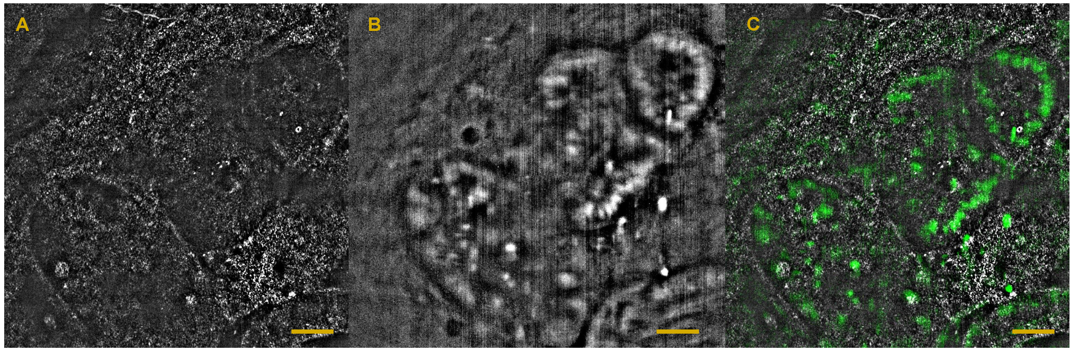
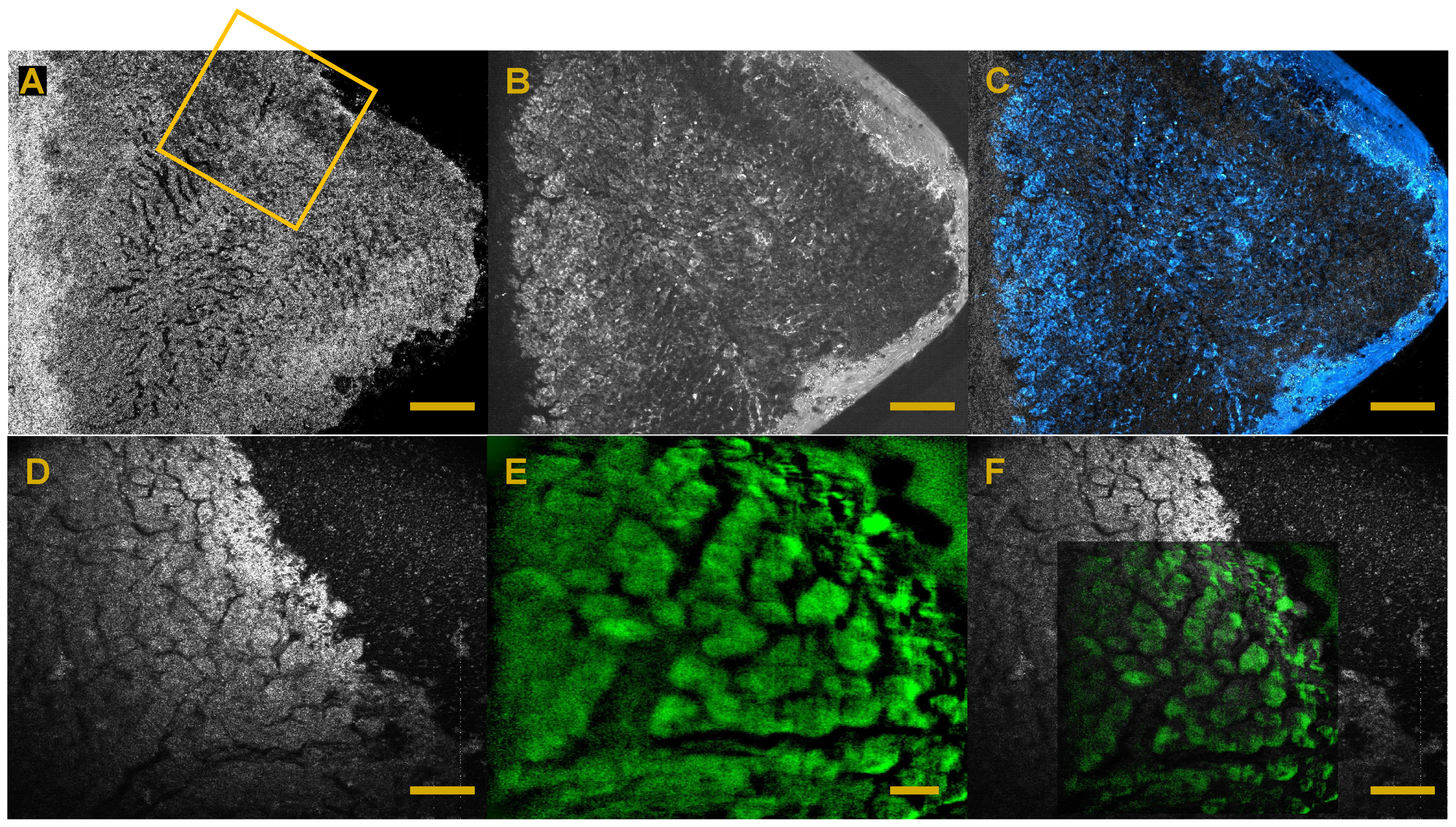
6. Full-Field OCT and Fluorescence

In principle, usual histology staining and fluorescence techniques are quite similar, except that fluorescence techniques use fluorescence probes instead of absorbing probes in histology. Some fluorescence techniques have been part of the histology toolkit for decades [136], such as immunofluorescence, which aims at detecting the interaction of a labeled antibody with a structure of interest [137], or fluorescence in situ hybridization (FISH) ([138,139], Chapter 6), which aims at detecting the interaction of a labeled nucleotide sequence with its specific complementary sequence in a cell. More recently, confocal microscopy [140] and two photon microscopy [141] have been used in order to detect fluorescent probes in depth in tissues. Interestingly, thanks to the optical sectioning provided by these techniques, it has become possible to follow some fluorescent structures in ex vivo tissues, and in vivo [142,143].

However, fluorescence techniques still require fluorescent labels, that need to be injected in the tissue. It can take a long time before the label diffuses in depth inside a tissue. Moreover, and similarly to classic histology stains, these labels only tag a few structures of interest, and it might be hard to understand the organization of these structures inside their microenvironment. Multiple labeling can be used to tag several structures, but it increases the complexity, and the cost of such experiments.

We can also add that usually, confocal and two photon microscopy can only access shallow depth inside a tissue, down to a few hundred $\mathsf{\mu }$m at best. OCT techniques on the other hand can access deeper regions down to one millimeter, since the signal is often enhanced by the reference arm. Recently, clearing techniques [144,145] with low tissue distortions have been developed in order to increase tissue transparency, and to image through the entire tissue. OCT can also benefit from these approaches [146], even if we would expect the intrinsic signal to be reduced in OCT, since clearing tends to remove lipid structures and to average the refractive index fluctuations. However, it can help to detect exogenous OCT contrast agent at important depths, such as metallic nanoparticles. Here again, clearing processes are often long, and can induce tissue distortions.

Fluorescence and OCT techniques are quite complementary, and multimodal systems combining the two can help with diagnosis, as we will illustrate throughout this section. Many such multimodal setups have been developed with both scanning OCT approaches [5,147] and full-field approaches, using either a flip mirror to switch from one modality to the other [18,148], or a simultaneous approach [41,42]. If all these multimodal approaches share a common interest, scanning OCT approaches are more easily combined with scanning fluorescence approaches, such as confocal or two photon microscopies, whereas FF-OCT systems have been developed in combination with widefield fluorescence techniques, such as structured illumination microscopy (SIM). SIM acquisition speed intrinsically depends on the fluorescence camera frame rate divided by the number of grid modulation steps. The SIM acquisition rate can go up to 100 frames per second in our measurements, even though the usual frame rate limit comes from the fluorophores’ brightness, and from the minimal exposure time required to produce a decent image. Interestingly, simultaneous combination of FF-OCT and SIM [41,42] enable the parallel acquisition of both modalities, so images with both modalities can be acquired at more than 100 frames per second. However, SIM is not very robust to aberrations and multiple scattering, and can hardly penetrate inside scattering samples after 30 to 50 $\mathsf{\mu }$m. Nevertheless, in mostly transparent samples, such as cornea or retina, with only a few structures labeled, we could perform multimodal FF-OCT and SIM images through the entire sample.

The first interest of combining OCT with fluorescence is to identify structures that are captured in OCT, in order to better understand and characterize OCT contrast [62]. The second interest is to use fluorescence to reveal some structures, proteins, or ultimately any structure that cannot be captured by OCT, therefore combining fluorescence molecular contrast with structural contrast from OCT. It can help to understand how a structure of interest integrates and evolves inside its micro environment, such as neurons in the intestine [149], or to find the location of stem cells in the cornea [12]. Figure 7 shows the example of imaging a tumorous intestine tissue, in which cell nuclei are labeled with fluorescence. This image shows the complementary contrast that can be obtained with both modalities. Additionally, with both sources of information, we can localize the cells on the contours of organized structures, named intestine villi, indicating that this field of view has been acquired in a healthy region of the cancerous tissue.

A final interest, that is often neglected, especially in the context of histology, is that fluorescence enables dynamic measurements that can probe the tissue biochemistry and its evolution, using specific probes. For examples, fluorescence measurements can follow the electrical activity of cells by quantitatively measuring their intracellular calcium concentration [150,151], or directly measure the membrane potential [152]. It can be useful to assess the viability of a cortical or retinal explant from its spontaneous activity, or can assess the endocrine pancreatic function, as insulin production is triggered by calcium uptake. Fluorescence can also directly measure cell function by measuring the intracellular ATP concentration [153], and can specifically detect apoptotic cells, with the ClickIt TUNEL assay (ThermoFisher). This can be of major importance to study the efficiency of pharmaceuticals on a cancerous tissue, as the cellular recovery of apoptosis within the tumor is usually a promising sign of a treatment’s success.

Figure 8 shows the result of the ClickIt TUNEL assay (from ThermoFisher Scientific [154]) on a fresh liver tissue. The tissue is first purposely excised with a corner shape to elicit and follow the cell death propagation from the margin to the center of the tissue. After several minutes, the tissue is imaged with FF-OCT and D-FF-OCT, and an inactive region (dark region from the tissue margin) can be detected with D-FF-OCT (panels A to C). Directly after the imaging, the tissue is fixed, in order to start the TUNEL assay and detect the apoptotic regions of this tissue. Unfortunately, this assay requires fixed tissues, so we cannot overlay a D-FF-OCT, and a fluorescence image. However, we could detect that almost all cells in a 200 $\mathsf{\mu }$m region from the tissue border were in apoptosis (panels D to F). The fluorescence signal started decreasing as we went further from the tissue margin, and is almost equal to zero at the center of the tissue. Figure 8 tends to show that apoptotic cells do not produce a dynamic contrast, at least for cells in apoptosis for a long time. Surprisingly, this indirect result is different from what was obtained with OCT measurements [155], where the authors showed a decrease of the speckle decorrelation time (i.e., an increase of the intracellular activity) in apoptotic cells. Explanations for this result may be the following: In contrast to G.Farhat et al. [155], we used a brute force method to generate apoptosis, as we physically cut the sample, and imaged close to the tissue edge. It is likely that the cells in the dark D-FF-OCT region are in late stages of apoptosis. Moreover, since cells in apoptosis tend to dilute and homogenize their intracellular material [156], it should lower the backscattered signal from the cell to a level that may be beneath our system detection limit, thus creating a dark D-FF-OCT image, even if the dynamics have increased.

7. Comparison with Other Popular Novel Microscopies

As previously pointed out, although fixation and labeling protocols have been greatly improved these past years in histology, this field could still benefit from the important technological developments that optical imaging has known over the past twenty years. So far, we compared FF-OCT and its multimodal versions to standard histology procedures. However, to be fair, we should also compare them to other recently developed optical techniques, such as multiphoton microscopies, and coherent anti-Stokes Raman scattering (CARS) microscopy, that also are label-free and enable optical sectioning. Similarly to OCT, these techniques rely on the intrinsic properties of tissues to generate contrast. They both can provide optical sectioning, since they rely on the combination of two or three photons, that can statistically only happen at the focal plane where the power density is high enough. Second harmonic generation (SHG) is measured in dense non-centrosymmetric structures, such as microtubule bundles, and collagen I fibers [157]. Third harmonic generation (THG) is measured at interfaces displaying high index mismatch, such as cell or nuclear contours, and lipid droplets [158]. Both techniques, especially when combined, are therefore useful to study 3D tissue organization, e.g., in the cornea [159], or in developing embryos [160]. The association of the two techniques gives a contrast similar to FF-OCT, but non-linear microscopes are a little more sensitive and specific than the FF-OCT signal, and can be naturally combined with two-photon fluorescence microscopy [161]. The transverse resolution is often higher than FF-OCT, as high NA objectives are required to generate a high power density at the focal point. We can add that SHG has already been extensively used to assess tissue disorganization, especially in the context of liver fibrosis [162]. A commercial SHG microscope for histology is already available at HistoIndex [163].

CARS [164], and its hyperspectral version [165], are other promising non-linear techniques for histology, which reveal a high density of either a single or multiple molecular vibrations inside a sample. Interestingly, CARS is one of the only techniques that is both label-free, and specific at the molecular level, as vibration spectra of given structures can be measured, and computationally extracted [166]. It is therefore one of the most promising label-free techniques today for quantification of tissue structure, and molecular content. Unfortunately, to our knowledge, there is no commercial CARS system available, and CARS systems often require careful and time consuming alignment steps.

Finally, we can add that all these techniques are based on non-linear processes that require similar kinds of sources, i.e., femtosecond lasers, and can be ingeniously combined all together from a single laser source [167]. However, such non-linear processes are quite weak. They typically display a low signal-to-noise ratio, especially in dense tissues, and often require long exposure times to generate a measurable signal. Combined with high NA objectives, the measurable field of view within one hour of imaging is fairly limited. Additionally, femtosecond lasers are expensive, especially compared with FF-OCT sources that are simple thermal light or LEDs. Finally, as non-linear processes, SHG, THG, and CARS signals are mainly forward scattered, so they often have to be used within thin tissue sections (a few hundred microns to 1 mm). We can nevertheless note that multiple scattering happening in highly scattering tissues allows the observation of non-linear processes in an epi configuration [164].

FF-OCT appears better suited than competing techniques for fast imaging of large tissue volumes in the operating room, to complement frozen-section histology procedures.

8. Conclusions and Perspectives

Full-field optical coherence tomography is a modified version of OCT that can access submicrometric resolution deep inside a sample. Similarly to OCT, it can provide label-free 3D imaging of ex vivo tissues, and can perform measurements similar to histology in terms of contrast and resolution. The interest of FF-OCT lies in its ability to obtain 3D images similar to histology with almost no tissue preparation, which can reduce slicing, staining, and fixation artifacts. FF-OCT can also significantly shorten the biopsy-to-diagnosis time, down to a few minutes. Unfortunately, FF-OCT diagnosis scores are not yet 100% when compared with histology. In this review, we highlighted three promising recent multimodal systems combining FF-OCT structural contrast with other specific contrasts such as mechanical, motility, and molecular contrasts, providing hope that FF-OCT diagnosis scores will increase in the future, and might even ultimately perform better than histology. We need to add that despite our choice here, there are other promising multimodal systems that could be of interest for diagnosis improvement. For example, polarization FF-OCT [21] can be used to increase the sensitivity to fibers, and should be able to detect fiber disorganizations, similarly to OCT measurements, e.g., that could detect polarization changes caused by age-related macular degeneration (AMD) or glaucoma [168]. Multicolor FF-OCT [22] might also help the detection of subtle wavelength-dependent scattering changes, related to tumor malignancy [69].

Despite all these exciting developments, and the possibility to combine many different modalities in a single optical system, we have to emphasize that a compromise will have to be found between speed, processing time, compactness, penetration depth and the number of contrasts available, especially when FF-OCT is used during surgery. We believe that a better characterization of FF-OCT (and D-FF-OCT) contrasts that would be performed specifically for each tissue would help to increase FF-OCT diagnosis ability, without even changing the optical design of the microscope.

Beyond the scope of histology, we hope that the development of such multimodal systems will increase the potential interest in FF-OCT, not only as an ex vivo diagnosis tool, but also as a tool to answer complex biological questions. We showed in this article that FF-OCT reveals a label-free original contrast, and can be used either in ex vivo tissues, or in vivo in small animals. If scanning OCT techniques were now to be extensively used in vivo and in clinics, FF-OCT would suffer from the slow speed of 2D detectors that do not allow a dynamic correction of the sample position, which could cancel the sample motion; in vivo implementation is therefore challenging. However, a few in vivo experiments have been successfully performed in paralyzed or anesthetized small animals [35,61], and in human skins pressed against an imaging window. We recently successfully performed a simultaneous FF-OCT, D-FF-OCT, and fluorescence measurement in living zebrafish larvae. We illustrate our ability to obtain a motility contrast in vivo, even in the presence of blood flow in Figure 9. The dynamic signal is saturated in the blood vessels, and below, but cells can be detected in between the vessels. Additionally, an important effort is being made to enable FF-OCT measurements in patients, with the recent development of two adaptive optics FF-OCT systems [169,170] for retinal imaging, a FF-OCT system coupled with an OCT system to dynamically compensate for eye motion for cornea and retina assessment, and a dark field FF-OCT system [171] to record internal fingerprints. Additionally, our group recently developed an en face matrix based approach of OCT, which allows to increase the penetration depth by a factor of two [172], and could be advantageous for in vivo experiments.

Finally, we are now interested in the development of functional imaging in FF-OCT, in fresh tissues, or in living animals, either by measuring changes in the blood flow, similarly to what has been achieved in OCT [132,173], or by directly measuring changes in the tissue biomechanics, or cellular activity. We believe that diagnosis capabilities will further benefit from this research, since it might soon be possible not only to detect static structural changes in a tissue, but also to detect how it reacts to different stimuli, or different drugs.

References

1. Drexler, W.; Fujimoto, J.G. Optical Coherence Tomography: Technology and Applications, 2nd ed.; Springer: Gewerbestrasse, Switzerland, 2015. [Google Scholar]
2. Zaitsev, V.Y.; Vitkin, I.A.; Matveev, L.A.; Gelikonov, V.M.; Matveyev, A.L.; Gelikonov, G.V. Recent Trends in Multimodal Optical Coherence Tomography. II. The Correlation-Stability Approach in OCT Elastography and Methods for Visualization of Microcirculation. Radiophys. Quant. Electron. 2014, 57, 210–225. [Google Scholar] [CrossRef]
3. Zaitsev, V.Y.; Gelikonov, V.M.; Matveev, L.A.; Gelikonov, G.V.; Matveyev, A.L.; Shilyagin, P.A.; Vitkin, I.A. Recent trends in multimodal optical coherence tomography. I. Polarization-sensitive oct and conventional approaches to OCT elastography. Radiophys. Quant. Electron. 2014, 57, 52–66. [Google Scholar] [CrossRef]
4. Oldenburg, A.L.; Chhetri, R.K.; Cooper, J.M.; Wu, W.C.; Troester, M.A.; Tracy, J.B. Motility-, autocorrelation-, and polarization-sensitive optical coherence tomography discriminates cells and gold nanorods within 3D tissue cultures. Opt. Lett. 2013, 38, 2923–2926. [Google Scholar] [CrossRef] [PubMed]
5. Beaurepaire, E.; Moreaux, L.; Amblard, F.; Mertz, J. Combined scanning optical coherence and two-photon-excited fluorescence microscopy. Opt. Lett. 1999, 24, 969–971. [Google Scholar] [CrossRef] [PubMed]
6. Beaurepaire, E.; Boccara, A.C.; Lebec, M.; Blanchot, L.; Saint-Jalmes, H. Full-field optical coherence microscopy. Opt. Lett. 1998, 23, 244–246. [Google Scholar] [CrossRef] [PubMed]
7. Dubois, A.; Vabre, L.; Boccara, A.C.; Beaurepaire, E. High-resolution full-field optical coherence tomography with a Linnik microscope. Appl. Opt. 2002, 41, 805–812. [Google Scholar] [CrossRef] [PubMed]
8. Jain, M.; Shukla, N.; Manzoor, M.; Nadolny, S.; Mukherjee, S. Modified full-field optical coherence tomography: A novel tool for rapid histology of tissues. J. Pathol. Inf. 2011, 2, 28. [Google Scholar]
9. Grieve, K.; Mouslim, K.; Assayag, O.; Dalimier, E.; Harms, F.; Bruhat, A.; Boccara, C.; Antoine, M. Assessment of Sentinel Node Biopsies With Full-Field Optical Coherence Tomography. Technol. Cancer Res. Treat. 2016, 15, 266–274. [Google Scholar] [CrossRef] [PubMed]
10. De Leeuw, F.; Casiraghi, O.; Lakhdar, A.B.; Abbaci, M.; Laplace-Builhé, C. Full-field OCT for fast diagnostic of head and neck cancer. In Proceedings of the SPIE BiOS, San Francisco, CA, USA, 7–12 February 2015; p. 93031Z.
11. Yang, C.; Ricco, R.; Sisk, A.; Duc, A.; Sibony, M.; Beuvon, F.; Dalimier, E.; Delongchamps, N.B. High efficiency for prostate biopsy qualification with full-field OCT after training. In Proceedings of the SPIE BiOS, San Francisco, CA, USA, 13–18 February 2016; p. 96891J.
12. Grieve, K.; Georgeon, C.; Andreiuolo, F.; Borderie, M.; Ghoubay, D.; Rault, J.; Borderie, V.M. Imaging Microscopic Features of Keratoconic Corneal Morphology. Cornea 2016, 35, 1621. [Google Scholar] [CrossRef] [PubMed]
13. Assayag, O.; Grieve, K.; Devaux, B.; Harms, F.; Pallud, J.; Chretien, F.; Boccara, C.; Varlet, P. Imaging of non-tumorous and tumorous human brain tissues with full-field optical coherence tomography. NeuroImage Clin. 2013, 2, 549–557. [Google Scholar] [CrossRef] [PubMed]
14. Assayag, O.; Antoine, M.; Sigal-Zafrani, B.; Riben, M.; Harms, F.; Burcheri, A.; Grieve, K.; Dalimier, E.; de Poly, B.L.C.; Boccara, C. Large field, high resolution full-field optical coherence tomography: A pre-clinical study of human breast tissue and cancer assessment. Technol. Cancer Res. Treat. 2014, 13, 455–468. [Google Scholar] [CrossRef] [PubMed]
15. Peters, I.T.A.; Stegehuis, P.L.; Peek, R.; Boer, F.L.; Zwet, E.W.V.; Eggermont, J.; Westphal, J.R.; Kuppen, P.J.K.; Trimbos, J.B.M.Z.; Hilders, C.G.J.M.; et al. Non-invasive detection of metastases and follicle density in ovarian tissue using full-field optical coherence tomography. Clin. Cancer Res. 2016. [Google Scholar] [CrossRef] [PubMed]
16. Handbook of Full-Field Optical Coherence Microscopy: Technology and Applications; Pan Stanford Publishing Pte. Ltd.: Singapore, 2016.
17. Jain, M.; Robinson, B.D.; Salamoon, B.; Thouvenin, O.; Boccara, C.; Mukherjee, S. Rapid evaluation of fresh ex vivo kidney tissue with full-field optical coherence tomography. J. Pathol. Inf. 2015, 6. [Google Scholar] [CrossRef] [PubMed]
18. Auksorius, E.; Bromberg, Y.; Motiejūnaitė, R.; Pieretti, A.; Liu, L.; Coron, E.; Aranda, J.; Goldstein, A.M.; Bouma, B.E.; Kazlauskas, A.; et al. Dual-modality fluorescence and full-field optical coherence microscopy for biomedical imaging applications. Biomed. Opt. Express 2012, 3, 661–666. [Google Scholar] [CrossRef] [PubMed] [Green Version]
19. Nahas, A.; Varna, M.; Fort, E.; Boccara, A.C. Detection of plasmonic nanoparticles with full field-OCT: Optical and photothermal detection. Biomed. Opt. Express 2014, 5, 3541–3546. [Google Scholar] [CrossRef] [PubMed]
20. Nahas, A.; Bauer, M.; Roux, S.; Boccara, A.C. 3D static elastography at the micrometer scale using Full Field OCT. Biomed. Opt. Express 2013, 4, 2138–2149. [Google Scholar] [CrossRef] [PubMed]
21. Moneron, G.; Boccara, A.C.; Dubois, A. Polarization-sensitive full-field optical coherence tomography. Opt. Lett. 2007, 32, 2058–2060. [Google Scholar] [CrossRef] [PubMed]
22. Yu, L.; Kim, M. Full-color three-dimensional microscopy by wide-field optical coherence tomography. Opt. Express 2004, 12, 6632–6641. [Google Scholar] [CrossRef] [PubMed]
23. Federici, A.; Dubois, A. Three-band, 1.9-μm axial resolution full-field optical coherence microscopy over a 530–1700 nm wavelength range using a single camera. Opt. Lett. 2014, 39, 1374–1377. [Google Scholar] [CrossRef] [PubMed]
24. Dubois, A.; Moreau, J.; Boccara, C. Spectroscopic ultrahigh-resolution full-field optical coherence microscopy. Opt. Express 2008, 16, 17082–17091. [Google Scholar] [CrossRef] [PubMed]
25. Huang, D.; Swanson, E.A.; Lin, C.P.; Schuman, J.S.; Stinson, W.G.; Chang, W.; Hee, M.R.; Flotte, T.; Gregory, K.; Puliafito, C.A.; et al. Optical coherence tomography. Science 1991, 254, 1178. [Google Scholar] [CrossRef] [PubMed]
26. Izatt, J.A.; Swanson, E.A.; Fujimoto, J.G.; Hee, M.R.; Owen, G.M. Optical coherence microscopy in scattering media. Opt. Lett. 1994, 19, 590–592. [Google Scholar] [CrossRef] [PubMed]
27. Fercher, A.F.; Hitzenberger, C.K.; Kamp, G.; El-Zaiat, S.Y. Measurement of intraocular distances by backscattering spectral interferometry. Opt. Commun. 1995, 117, 43–48. [Google Scholar] [CrossRef]
28. De Boer, J.F.; Cense, B.; Park, B.H.; Pierce, M.C.; Tearney, G.J.; Bouma, B.E. Improved signal-to-noise ratio in spectral-domain compared with time-domain optical coherence tomography. Opt. Lett. 2003, 28, 2067–2069. [Google Scholar] [CrossRef] [PubMed]
29. Pircher, M.; Götzinger, E.; Hitzenberger, C.K. Dynamic focus in optical coherence tomography for retinal imaging. J. Biomed. Opt. 2006, 11, 054013. [Google Scholar] [CrossRef] [PubMed]
30. Holmes, J.; Hattersley, S.; Stone, N.; Bazant-Hegemark, F.; Barr, H. Multi-channel Fourier domain OCT system with superior lateral resolution for biomedical applications. In Proceedings of the Biomedical Optics (BiOS), San Jose, CA, USA, 19–24 January 2008; p. 68470O.
31. Ding, Z.; Ren, H.; Zhao, Y.; Nelson, J.S.; Chen, Z. High-resolution optical coherence tomography over a large depth range with an axicon lens. Opt. Lett. 2002, 27, 243–245. [Google Scholar] [CrossRef] [PubMed]
32. Ralston, T.S.; Marks, D.L.; Carney, P.S.; Boppart, S.A. Interferometric synthetic aperture microscopy. Nat. Phys. 2007, 3, 129–134. [Google Scholar] [CrossRef] [PubMed]
33. Kazmi, S.S.; Wu, R.K.; Dunn, A.K. Evaluating multi-exposure speckle imaging estimates of absolute autocorrelation times. Opt. Lett. 2015, 40, 3643–3646. [Google Scholar] [CrossRef] [PubMed]
34. Potsaid, B.; Gorczynska, I.; Srinivasan, V.J.; Chen, Y.; Jiang, J.; Cable, A.; Fujimoto, J.G. Ultrahigh speed spectral/Fourier domain OCT ophthalmic imaging at 70,000 to 312,500 axial scans per second. Opt. Express 2008, 16, 15149–15169. [Google Scholar] [CrossRef] [PubMed]
35. Grieve, K.; Dubois, A.; Simonutti, M.; Paques, M.; Sahel, J.; Le Gargasson, J.F.; Boccara, C. In vivo anterior segment imaging in the rat eye with high speed white light full-field optical coherence tomography. Opt. Express 2005, 13, 6286–6295. [Google Scholar] [CrossRef] [PubMed]
36. Song, S.; Huang, Z.; Nguyen, T.M.; Wong, E.Y.; Arnal, B.; O’Donnell, M.; Wang, R.K. Shear modulus imaging by direct visualization of propagating shear waves with phase-sensitive optical coherence tomography. J. Biomed. Opt. 2013, 18, 121509. [Google Scholar] [CrossRef] [PubMed]
37. Commercial System LLTech. Avaiable online: http://www.lltechimaging.com/products-applications/products/ (accessed on 20 January 2017).
38. Nahas, A.; Tanter, M.; Nguyen, T.M.; Chassot, J.M.; Fink, M.; Boccara, A.C. From supersonic shear wave imaging to full-field optical coherence shear wave elastography. J. Biomed. Opt. 2013, 18, 121514. [Google Scholar] [CrossRef] [PubMed]
39. Apelian, C.; Harms, F.; Thouvenin, O.; Boccara, A.C. Dynamic full field optical coherence tomography: Subcellular metabolic contrast revealed in tissues by temporal analysis of interferometric signals. arXiv, 2016; arXiv:1601.01208. [Google Scholar] [CrossRef] [PubMed]
40. Leroux, C.E.; Bertillot, F.; Thouvenin, O.; Boccara, A.C. Intracellular dynamics measurements with full field optical coherence tomography suggest hindering effect of actomyosin contractility on organelle transport. Biomed. Opt. Express 2016, 7, 4501–4513. [Google Scholar] [CrossRef] [PubMed]
41. Thouvenin, O.; Fink, M.; Boccara, C. Dynamic multimodal full-field optical coherence tomography and fluorescence structured illumination microscopy. J. Biomed. Opt. 2017, 22, 026004. [Google Scholar] [CrossRef] [PubMed]
42. Makhlouf, H.; Perronet, K.; Dupuis, G.; Lévêque-Fort, S.; Dubois, A. Simultaneous optically sectioned fluorescence and optical coherence microscopy with full-field illumination. Opt. Lett. 2012, 37, 1613–1615. [Google Scholar] [CrossRef] [PubMed]
43. Abdulhalim, I. Spatial and temporal coherence effects in interference microscopy and full-field optical coherence tomography. Ann. Phys. 2012, 524, 787–804. [Google Scholar] [CrossRef]
44. Dubois, A.; Selb, J.; Vabre, L.; Boccara, A.C. Phase measurements with wide-aperture interferometers. Appl. Opt. 2000, 39, 2326–2331. [Google Scholar] [CrossRef] [PubMed]
45. Karamata, B.; Lambelet, P.; Laubscher, M.; Salathé, R.; Lasser, T. Spatially incoherent illumination as a mechanism for cross-talk suppression in wide-field optical coherence tomography. Opt. Lett. 2004, 29, 736–738. [Google Scholar] [CrossRef] [PubMed]
46. Xiao, P.; Fink, M.; Boccara, A.C. Full-field spatially incoherent illumination interferometry: A spatial resolution almost insensitive to aberrations. Opt. Lett. 2016, 41, 3920–3923. [Google Scholar] [CrossRef] [PubMed]
47. CMOSIS New Camera by Adimec. Avaiable online: http://info.adimec.com/blogposts/careioca-project-results-in-several-new-products-including-cmosis-csi2100-adimec-q-2a750-and-lltech-ffoct-microscope-and-endoscope (accessed on 20 January 2017).
48. Mandrioli, P.; Ariatti, A. Marcello Malpighi, a pioneer of the experimental research in biology. Aerobiologia 1991, 7, 3–9. [Google Scholar] [CrossRef]
49. Reverón, R.R. Marcello Malpighi (1628–1694), founder of microanatomy. Int. J. Morphol. 2011, 29, 399–402. [Google Scholar] [CrossRef]
50. Cohen, A.L.; Hayat, M.A. Principles and Techniques of Scanning Electron Microscopy. Biological Applications. Volume 1; Van Nostrand Reinhold Company: Cincinatti, OH, USA, 1974. [Google Scholar]
51. Digital Microscope. Avaiable online: http://www.histology.be/digital_microscope_histology_.html (accessed on 20 January 2017).
52. Histology Guide: Virtual Histology Lab. Avaiable online: http://histologyguide.org/index.html (accessed on 20 January 2017).
53. Amunts, K.; Lepage, C.; Borgeat, L.; Mohlberg, H.; Dickscheid, T.; Rousseau, M.É.; Bludau, S.; Bazin, P.L.; Lewis, L.B.; Oros-Peusquens, A.M.; et al. BigBrain: An ultrahigh-resolution 3D human brain model. Science 2013, 340, 1472–1475. [Google Scholar] [CrossRef] [PubMed]
54. Leslie, P.; Gartner, L.P. Color Atlas and Text of Histology, 6th ed.; Lippincott Williams and Wilkins: Philadelphia, PA, USA, 2013. [Google Scholar]
55. Auth, A.C. A Text-Book of Histology. Descriptive and Practical. For the Use of Students; John Wright and Co.: Bristol, UK, 1986. [Google Scholar]
56. Spitalnik, P.F. Histology Lab Manual; Columbia University: New York, NY, USA, 2015. [Google Scholar]
57. Clinical Atlas LLTech. Avaiable online: http://www.lltechimaging.com/image-gallery/atlas-of-images/ (accessed on 20 January 2017).
58. Magnain, C.; Augustinack, J.C.; Konukoglu, E.; Frosch, M.P.; Sakadžić, S.; Varjabedian, A.; Garcia, N.; Wedeen, V.J.; Boas, D.A.; Fischl, B. Optical coherence tomography visualizes neurons in human entorhinal cortex. Neurophotonics 2015, 2, 015004. [Google Scholar] [CrossRef] [PubMed]
59. Wang, H.; Zhu, J.; Akkin, T. Serial optical coherence scanner for large-scale brain imaging at microscopic resolution. Neuroimage 2014, 84, 1007–1017. [Google Scholar] [CrossRef] [PubMed]
60. Quinten, M. Optical Properties of Nanoparticle Systems: Mie and Beyond; John Wiley & Sons: Hoboken, NJ, USA, 2010. [Google Scholar]
61. Arous, J.B.; Binding, J.; Léger, J.F.; Casado, M.; Topilko, P.; Gigan, S.; Boccara, A.C.; Bourdieu, L. Single myelin fiber imaging in living rodents without labeling by deep optical coherence microscopy. J. Biomed. Opt. 2011, 16, 116012. [Google Scholar] [CrossRef] [PubMed]
62. Grieve, K.; Thouvenin, O.; Sengupta, A.; Borderie, V.M.; Paques, M. Appearance of the Retina With Full-Field Optical Coherence Tomography. Investig. Opthalmol. Vis. Sci. 2016, 57, OCT96. [Google Scholar] [CrossRef] [PubMed]
63. Wang, S.; Liu, C.H.; Zakharov, V.P.; Lazar, A.J.; Pollock, R.E.; Larin, K.V. Three-dimensional computational analysis of optical coherence tomography images for the detection of soft tissue sarcomas. J. Biomed. Opt. 2014, 19, 0211022. [Google Scholar] [CrossRef] [PubMed]
64. Boppart, S.A.; Luo, W.; Marks, D.L.; Singletary, K.W. Optical coherence tomography: Feasibility for basic research and image-guided surgery of breast cancer. Breast Cancer Res. Treat. 2004, 84, 85–97. [Google Scholar] [CrossRef] [PubMed]
65. McLaughlin, R.A.; Scolaro, L.; Robbins, P.; Hamza, S.; Saunders, C.; Sampson, D.D. Imaging of human lymph nodes using optical coherence tomography: Potential for staging cancer. Cancer Res. 2010, 70, 2579–2584. [Google Scholar] [CrossRef] [PubMed]
66. Vakoc, B.J.; Fukumura, D.; Jain, R.K.; Bouma, B.E. Cancer imaging by optical coherence tomography: Preclinical progress and clinical potential. Nat. Rev. Cancer 2012, 12, 363–368. [Google Scholar] [CrossRef] [PubMed]
67. Sharma, M.; Verma, Y.; Rao, K.; Nair, R.; Gupta, P. Imaging growth dynamics of tumour spheroids using optical coherence tomography. Biotechnol. Lett. 2007, 29, 273–278. [Google Scholar] [CrossRef] [PubMed]
68. Yang, Y.; Wang, T.; Biswal, N.C.; Wang, X.; Sanders, M.; Brewer, M.; Zhu, Q. Optical scattering coefficient estimated by optical coherence tomography correlates with collagen content in ovarian tissue. J. Biomed. Opt. 2011, 16, 090504. [Google Scholar] [CrossRef] [PubMed]
69. Vakoc, B.J.; Lanning, R.M.; Tyrrell, J.A.; Padera, T.P.; Bartlett, L.A.; Stylianopoulos, T.; Munn, L.L.; Tearney, G.J.; Fukumura, D.; Jain, R.K.; et al. Three-dimensional microscopy of the tumor microenvironment in vivo using optical frequency domain imaging. Nat. Med. 2009, 15, 1219–1223. [Google Scholar] [CrossRef] [PubMed]
70. Sullivan, A.C.; Hunt, J.P.; Oldenburg, A.L. Fractal analysis for classification of breast carcinoma in optical coherence tomography. J. Biomed. Opt. 2011, 16, 066010. [Google Scholar] [CrossRef] [PubMed]
71. Gao, W.; Zhu, Y. Fractal analysis of en face tomographic images obtained with full field optical coherence tomography. Ann. Phys. 2016, 93. [Google Scholar] [CrossRef]
72. Nicolson, M. The art of diagnosis: Medicine and the five senses. In Companion Encyclopedia of the History of Medicine, Volume 2; Bynum, W., Porter, R., Eds.; Routledge: London, UK, 1997; pp. 801–825. [Google Scholar]
73. Medical Diagnosis in Egyptian World. Available online: http://www.arabworldbooks.com/articles8.htm (accessed on 20 January 2017).
74. Sarvazyan, A. Shear acoustic properties of soft biological tissues in medical diagnostics. J. Acoust. Soc. Am. 1993, 93, 2329–2330. [Google Scholar] [CrossRef]
75. Bataller, R.; Brenner, D.A. Liver fibrosis. J. Clin. Investig. 2005, 115, 209–218. [Google Scholar] [CrossRef] [PubMed]
76. Mueller, S.; Sandrin, L. Liver stiffness: A novel parameter for the diagnosis of liver disease. Hepat. Med. 2010, 2, 49–67. [Google Scholar] [CrossRef] [PubMed]
77. Kumar, S.; Weaver, V.M. Mechanics, malignancy, and metastasis: The force journey of a tumor cell. Cancer Metastasis Rev. 2009, 28, 113–127. [Google Scholar] [CrossRef] [PubMed]
78. Mouw, J.K.; Yui, Y.; Damiano, L.; Bainer, R.O.; Lakins, J.N.; Acerbi, I.; Ou, G.; Wijekoon, A.C.; Levental, K.R.; Gilbert, P.M.; et al. Tissue mechanics modulate microRNA-dependent PTEN expression to regulate malignant progression. Nat. Med. 2014, 20, 360. [Google Scholar] [CrossRef] [PubMed]
79. Ophir, J.; Cespedes, I.; Ponnekanti, H.; Yazdi, Y.; Li, X. Elastography: A quantitative method for imaging the elasticity of biological tissues. Ultrason. Imaging 1991, 13, 111–134. [Google Scholar] [CrossRef] [PubMed]
80. Muthupillai, R.; Lomas, D.; Rossman, P.; Greenleaf, J.F.; Manduca, A.; Ehman, R.L. Magnetic resonance elastography by direct visualization of propagating acoustic strain waves. Science 1995, 269, 1854. [Google Scholar] [CrossRef] [PubMed]
81. Mariappan, Y.K.; Glaser, K.J.; Ehman, R.L. Magnetic resonance elastography: A review. Clin. Anat. 2010, 23, 497–511. [Google Scholar] [CrossRef] [PubMed]
82. Tanter, M.; Bercoff, J.; Athanasiou, A.; Deffieux, T.; Gennisson, J.L.; Montaldo, G.; Muller, M.; Tardivon, A.; Fink, M. Quantitative assessment of breast lesion viscoelasticity: Initial clinical results using supersonic shear imaging. Ultras. Med. Biol. 2008, 34, 1373–1386. [Google Scholar] [CrossRef] [PubMed]
83. Gayrard, C.; Borghi, N. FRET-based molecular tension microscopy. Methods 2016, 94, 33–42. [Google Scholar] [CrossRef] [PubMed]
84. Schmitt, J.M. OCT elastography: Imaging microscopic deformation and strain of tissue. Opt. Express 1998, 3, 199–211. [Google Scholar] [CrossRef] [PubMed]
85. Wang, R.K.; Ma, Z.; Kirkpatrick, S.J. Tissue Doppler optical coherence elastography for real time strain rate and strain mapping of soft tissue. Appl. Phys. Lett. 2006, 89, 144103. [Google Scholar] [CrossRef]
86. Kennedy, B.F.; Kennedy, K.M.; Sampson, D.D. A review of optical coherence elastography: Fundamentals, techniques and prospects. IEEE J. Sel. Top. Quant. Electron. 2014, 20, 272–288. [Google Scholar] [CrossRef]
87. Wang, S.; Larin, K.V. Optical coherence elastography for tissue characterization: A review. J. Biophoton. 2015, 8, 279–302. [Google Scholar] [CrossRef] [PubMed]
88. Mulligan, J.A.; Untracht, G.R.; Chandrasekaran, S.N.; Brown, C.N.; Adie, S.G. Emerging Approaches for High-Resolution Imaging of Tissue Biomechanics With Optical Coherence Elastography. IEEE J. Sel. Top. Quant. Electron. 2016, 22, 1–20. [Google Scholar] [CrossRef]
89. Royer, D.; Dieulesaint, E. Elastic Waves in Solids I: Free and Guided Propagation; Morgan, D.P., Translator; Springer: New York, NY, USA, 2000. [Google Scholar]
90. Sarvazyan, A.P.; Rudenko, O.V.; Swanson, S.D.; Fowlkes, J.B.; Emelianov, S.Y. Shear wave elasticity imaging: A new ultrasonic technology of medical diagnostics. Ultras. Med. Boil. 1998, 24, 1419–1435. [Google Scholar] [CrossRef]
91. Roux, S.; Hild, F.; Viot, P.; Bernard, D. Three-dimensional image correlation from X-ray computed tomography of solid foam. Compos. A Appl. Sci. Manuf. 2008, 39, 1253–1265. [Google Scholar] [CrossRef] [Green Version]
92. Leclerc, H.; Périé, J.N.; Hild, F.; Roux, S. Digital volume correlation: What are the limits to the spatial resolution? Mech. Ind. 2012, 13, 361–371. [Google Scholar] [CrossRef]
93. Basser, P.J.; Mattiello, J.; LeBihan, D. MR diffusion tensor spectroscopy and imaging. Biophys. J. 1994, 66, 259. [Google Scholar] [CrossRef]
94. Le Bihan, D.; Mangin, J.F.; Poupon, C.; Clark, C.A.; Pappata, S.; Molko, N.; Chabriat, H. Diffusion tensor imaging: Concepts and applications. J. Magn. Reson. Imaging 2001, 13, 534–546. [Google Scholar] [CrossRef] [PubMed]
95. Papadacci, C.; Tanter, M.; Pernot, M.; Fink, M. Ultrasound backscatter tensor imaging (BTI): Analysis of the spatial coherence of ultrasonic speckle in anisotropic soft tissues. IEEE Trans. Ultrason. Ferroelectr. Freq. Control 2014, 61, 986–996. [Google Scholar] [CrossRef] [PubMed]
96. Chatelin, S.; Bernal, M.; Deffieux, T.; Papadacci, C.; Flaud, P.; Nahas, A.; Boccara, C.; Gennisson, J.L.; Tanter, M.; Pernot, M. Anisotropic polyvinyl alcohol hydrogel phantom for shear wave elastography in fibrous biological soft tissue: A multimodality characterization. Phys. Med. Biol. 2014, 59, 6923. [Google Scholar] [CrossRef] [PubMed]
97. Kennedy, K.M.; Es’haghian, S.; Chin, L.; McLaughlin, R.A.; Sampson, D.D.; Kennedy, B.F. Optical palpation: Optical coherence tomography-based tactile imaging using a compliant sensor. Opt. Lett. 2014, 39, 3014–3017. [Google Scholar] [CrossRef] [PubMed]
98. Wellman, P.S.; Howe, R.D.; Dewagan, N.; Cundari, M.A.; Dalton, E.; Kern, K.A. Tactile imaging: A method for documenting breast masses. In Proceedings of the First Joint IEEE Engineering in Medicine and Biology, 21st Annual Conference and the 1999 Annual Fall Meetring of the Biomedical Engineering Society, Atlanta, GA, USA, 13–16 October 1999; Volume 2, p. 1131.
99. Razani, M.; Mariampillai, A.; Sun, C.; Luk, T.W.; Yang, V.X.; Kolios, M.C. Feasibility of optical coherence elastography measurements of shear wave propagation in homogeneous tissue equivalent phantoms. Biomed. Opt. Express 2012, 3, 972–980. [Google Scholar] [CrossRef] [PubMed]
100. Catheline, S.; Thomas, J.L.; Wu, F.; Fink, M.A. Diffraction field of a low frequency vibrator in soft tissues using transient elastography. IEEE Trans. Ultrason. Ferroelectr. Freq. Control 1999, 46, 1013–1019. [Google Scholar] [CrossRef] [PubMed]
101. Sandrin, L.; Catheline, S.; Tanter, M.; Hennequin, X.; Fink, M. Time-resolved pulsed elastography with ultrafast ultrasonic imaging. Ultrason. Imaging 1999, 21, 259–272. [Google Scholar] [CrossRef] [PubMed]
102. Bercoff, J.; Tanter, M.; Fink, M. Supersonic shear imaging: A new technique for soft tissue elasticity mapping. IEEE Trans. Ultrason. Ferroelectr. Freq. Control 2004, 51, 396–409. [Google Scholar] [CrossRef] [PubMed]
103. Chatelin, S.; Constantinesco, A.; Willinger, R. Fifty years of brain tissue mechanical testing: From in vitro to in vivo investigations. Biorheology 2010, 47, 255–276. [Google Scholar] [PubMed]
104. Macé, E.; Cohen, I.; Montaldo, G.; Miles, R.; Fink, M.; Tanter, M. In vivo mapping of brain elasticity in small animals using shear wave imaging. IEEE Trans. Med. Imaging 2011, 30, 550–558. [Google Scholar] [CrossRef] [PubMed]
105. Catheline, S.; Souchon, R.; Rupin, M.; Brum, J.; Dinh, A.; Chapelon, J.Y. Tomography from diffuse waves: Passive shear wave imaging using low frame rate scanners. Appl. Phys. Lett. 2013, 103, 014101. [Google Scholar] [CrossRef]
106. Zorgani, A.; Souchon, R.; Dinh, A.H.; Chapelon, J.Y.; Ménager, J.M.; Lounis, S.; Rouvière, O.; Catheline, S. Brain palpation from physiological vibrations using MRI. Proc. Natl. Acad. Sci. USA 2015, 112, 12917–12921. [Google Scholar] [CrossRef] [PubMed]
107. Nguyen, T.M.; Zorgani, A.; Lescanne, M.; Boccara, C.; Fink, M.; Catheline, S. Diffuse shear wave imaging: Toward passive elastography using low-frame rate spectral-domain optical coherence tomography. J. Biomed. Opt. 2016, 21, 126013. [Google Scholar] [CrossRef] [PubMed]
108. Pecora, R. Dynamic Light Scattering: Applications of Photon Correlation Spectroscopy; Springer Science & Business Media: Heidelberg, Germany, 2013. [Google Scholar]
109. Suissa, M.; Place, C.; Goillot, E.; Berge, B.; Freyssingeas, E. Dynamic light scattering as an investigating tool to study the global internal dynamics of a living cell nucleus. EPL Europhys. Lett. 2007, 78, 38005. [Google Scholar] [CrossRef]
110. Suissa, M.; Place, C.; Goillot, E.; Freyssingeas, E. Internal dynamics of a living cell nucleus investigated by dynamic light scattering. Eur. Phys. J. E 2008, 26, 435–448. [Google Scholar] [CrossRef] [PubMed]
111. Jeong, K.; Turek, J.J. Volumetric motility-contrast imaging of tissue response to cytoskeletal anti-cancer drugs. Opt. Express 2007, 15, 14057–14064. [Google Scholar] [CrossRef] [PubMed]
112. Nolte, D.D.; An, R.; Turek, J.; Jeong, K. Tissue dynamics spectroscopy for phenotypic profiling of drug effects in three-dimensional culture. Biomed. Opt. Express 2012, 3, 2825–2841. [Google Scholar] [CrossRef] [PubMed]
113. An, R.; Wang, C.; Turek, J.; Machaty, Z.; Nolte, D.D. Biodynamic imaging of live porcine oocytes, zygotes and blastocysts for viability assessment in assisted reproductive technologies. Biomed. Opt. Express 2015, 6, 963–976. [Google Scholar] [CrossRef] [PubMed]
114. Tan, W.; Oldenburg, A.L.; Norman, J.J.; Desai, T.A.; Boppart, S.A. Optical coherence tomography of cell dynamics in three-dimensional tissue models. Opt. Express 2006, 14, 7159–7171. [Google Scholar] [CrossRef] [PubMed]
115. Oldenburg, A.L.; Yu, X.; Gilliss, T.; Alabi, O.; Taylor, R.M.; Troester, M.A. Inverse-power-law behavior of cellular motility reveals stromal–epithelial cell interactions in 3D co-culture by OCT fluctuation spectroscopy. Optica 2015, 2, 877. [Google Scholar] [CrossRef] [PubMed]
116. Lee, J.; Wu, W.; Jiang, J.Y.; Zhu, B.; Boas, D.A. Dynamic light scattering optical coherence tomography. Opt. Express 2012, 20, 22262–22277. [Google Scholar] [CrossRef] [PubMed]
117. Chen, H.; Farkas, E.R.; Webb, W.W. In vivo applications of fluorescence correlation spectroscopy. Methods Cell Biol. 2008, 89, 3–35. [Google Scholar] [PubMed]
118. Tishler, R.B.; Carlson, F.D. A study of the dynamic properties of the human red blood cell membrane using quasi-elastic light-scattering spectroscopy. Biophys. J. 1993, 65, 2586. [Google Scholar] [CrossRef]
119. Miller, M.J.; Wei, S.H.; Parker, I.; Cahalan, M.D. Two-photon imaging of lymphocyte motility and antigen response in intact lymph node. Science 2002, 296, 1869–1873. [Google Scholar] [CrossRef] [PubMed]
120. Ammari, H.; Romero, F.; Shi, C. A signal separation technique for sub-cellular imaging using dynamic optical coherence tomography. arXiv, 2016; arXiv:1608.04382. [Google Scholar]
121. Demené, C.; Deffieux, T.; Pernot, M.; Osmanski, B.F.; Biran, V.; Gennisson, J.L.; Sieu, L.A.; Bergel, A.; Franqui, S.; Correas, J.M.; et al. Spatiotemporal clutter filtering of ultrafast ultrasound data highly increases Doppler and fUltrasound sensitivity. IEEE Trans. Med. Imaging 2015, 34, 2271–2285. [Google Scholar] [CrossRef] [PubMed]
122. Zink, D.; Fischer, A.H.; Nickerson, J.A. Nuclear structure in cancer cells. Nat. Rev. Cancer 2004, 4, 677–687. [Google Scholar] [CrossRef] [PubMed]
123. Slater, D.; Rice, S.; Stewart, R.; Melling, S.; Hewer, E.; Smith, J. Proposed Sheffield quantitative criteria in cervical cytology to assist the grading of squamous cell dyskaryosis, as the British Society for Clinical Cytology definitions require amendment. Cytopathology 2005, 16, 179–192. [Google Scholar] [CrossRef] [PubMed]
124. Popescu, G.; Park, Y.; Choi, W.; Dasari, R.R.; Feld, M.S.; Badizadegan, K. Imaging red blood cell dynamics by quantitative phase microscopy. Blood Cells Mol. Dis. 2008, 41, 10–16. [Google Scholar] [CrossRef] [PubMed]
125. Sato, E.; Olson, S.H.; Ahn, J.; Bundy, B.; Nishikawa, H.; Qian, F.; Jungbluth, A.A.; Frosina, D.; Gnjatic, S.; Ambrosone, C.; et al. Intraepithelial CD8+ tumor-infiltrating lymphocytes and a high CD8+/regulatory T cell ratio are associated with favorable prognosis in ovarian cancer. Proc. Natl. Acad. Sci. USA 2005, 102, 18538–18543. [Google Scholar] [CrossRef] [PubMed]
126. Mahmoud, S.M.; Paish, E.C.; Powe, D.G.; Macmillan, R.D.; Grainge, M.J.; Lee, A.H.; Ellis, I.O.; Green, A.R. Tumor-infiltrating CD8+ lymphocytes predict clinical outcome in breast cancer. J. Clin. Oncol. 2011, 29, 1949–1955. [Google Scholar] [CrossRef] [PubMed]
127. Weidner, N.; Carroll, P.; Flax, J.; Blumenfeld, W.; Folkman, J. Tumor angiogenesis correlates with metastasis in invasive prostate carcinoma. Am. J. Pathol. 1993, 143, 401. [Google Scholar] [PubMed]
128. Weidner, N. Current pathologic methods for measuring intratumoral microvessel density within breast carcinoma and other solid tumors. Breast Cancer Res. Treat. 1995, 36, 169–180. [Google Scholar] [CrossRef] [PubMed]
129. Maier, J.G.; Schamber, D.T. The role of lymphangiography in the diagnosis and treatment of malignant testicular tumors. Am. J. Roentgenol. 1972, 114, 482–491. [Google Scholar] [CrossRef]
130. Shaked, N.T.; Rinehart, M.T.; Wax, A. Quantitative phase microscopy of biological cell dynamics by wide-field digital interferometry. In Coherent Light Microscopy; Springer: Heidelberg, Germany, 2011; pp. 169–198. [Google Scholar]
131. Ma, L.; Rajshekhar, G.; Wang, R.; Bhaduri, B.; Sridharan, S.; Mir, M.; Chakraborty, A.; Iyer, R.; Prasanth, S.; Millet, L.; et al. Phase correlation imaging of unlabeled cell dynamics. Sci. Rep. 2016, 6. [Google Scholar] [CrossRef] [PubMed]
132. Berclaz, C.; Szlag, D.; Nguyen, D.; Extermann, J.; Bouwens, A.; Marchand, P.J.; Nilsson, J.; Schmidt-Christensen, A.; Holmberg, D.; Grapin-Botton, A.; et al. Label-free fast 3D coherent imaging reveals pancreatic islet micro-vascularization and dynamic blood flow. Biomed. Opt. Express 2016, 7, 4569–4580. [Google Scholar] [CrossRef] [PubMed]
133. Bouwens, A.; Szlag, D.; Szkulmowski, M.; Bolmont, T.; Wojtkowski, M.; Lasser, T. Quantitative lateral and axial flow imaging with optical coherence microscopy and tomography. Opt. Express 2013, 21, 17711–17729. [Google Scholar] [CrossRef] [PubMed]
134. Leitgeb, R.A.; Werkmeister, R.M.; Blatter, C.; Schmetterer, L. Doppler optical coherence tomography. Progr. Retin. Eye Res. 2014, 41, 26–43. [Google Scholar] [CrossRef] [PubMed]
135. Bouwens, A.; Bolmont, T.; Szlag, D.; Berclaz, C.; Lasser, T. Quantitative cerebral blood flow imaging with extended-focus optical coherence microscopy. Opt. Lett. 2014, 39, 37–40. [Google Scholar] [CrossRef] [PubMed]
136. Hicks, J.; Matthaei, E. Fluorescence in histology. J. Pathol. Bacteriol. 1955, 70, 1–12. [Google Scholar] [CrossRef] [PubMed]
137. John, D.; Bancroft, M.G. Theory and Practice Of Histological Techniques, 5th ed.; Churchill Livingstone: London, UK, 2002. [Google Scholar]
138. Volpi, E.V.; Bridger, J.M. FISH glossary: An overview of the fluorescence in situ hybridization technique. Biotechniques 2008, 45, 385–386. [Google Scholar] [CrossRef] [PubMed]
139. Roulston, J.E.; Bartlett, J.M. Molecular Diagnosis Of Cancer: Methods and Protocols; Springer Science & Business Media: New York, NY, USA, 2004; Volume 97. [Google Scholar]
140. Transidico, P.; Bianchi, M.; Capra, M.; Pelicci, P.G.; Faretta, M. From cells to tissues: Fluorescence confocal microscopy in the study of histological samples. Microsc. Res. Tech. 2004, 64, 89–95. [Google Scholar] [CrossRef] [PubMed]
141. Yuste, R. Fluorescence microscopy today. Nat. Methods 2005, 2, 902–904. [Google Scholar] [CrossRef] [PubMed]
142. Jung, J.C.; Mehta, A.D.; Aksay, E.; Stepnoski, R.; Schnitzer, M.J. In vivo mammalian brain imaging using one-and two-photon fluorescence microendoscopy. J. Neurophysiol. 2004, 92, 3121–3133. [Google Scholar] [CrossRef] [PubMed]
143. Flusberg, B.A.; Cocker, E.D.; Piyawattanametha, W.; Jung, J.C.; Cheung, E.L.; Schnitzer, M.J. Fiber-optic fluorescence imaging. Nat. Methods 2005, 2, 941–950. [Google Scholar] [CrossRef] [PubMed]
144. Tuchin, V.V. Optical clearing of tissues and blood using the immersion method. J. Phys. D Appl. Phys. 2005, 38, 2497. [Google Scholar] [CrossRef]
145. Chung, K.; Deisseroth, K. CLARITY for mapping the nervous system. Nat. Methods 2013, 10, 508–513. [Google Scholar] [CrossRef] [PubMed]
146. Larin, K.V.; Ghosn, M.G.; Bashkatov, A.N.; Genina, E.A.; Trunina, N.A.; Tuchin, V.V. Optical clearing for OCT image enhancement and in-depth monitoring of molecular diffusion. IEEE J. Sel. Top. Quant. Electron. 2012, 18, 1244–1259. [Google Scholar] [CrossRef]
147. Yuan, S.; Roney, C.A.; Wierwille, J.; Chen, C.W.; Xu, B.; Griffiths, G.; Jiang, J.; Ma, H.; Cable, A.; Summers, R.M.; Chen, Y. Co-registered optical coherence tomography and fluorescence molecular imaging for simultaneous morphological and molecular imaging. Phys. Med. Biol. 2010, 55, 191–206. [Google Scholar] [CrossRef] [PubMed]
148. Harms, F.; Dalimier, E.; Vermeulen, P.; Fragola, A.; Boccara, A. Multimodal Full-Field Optical Coherence Tomography on biological tissue: Toward all optical digital pathology. In Prcoeedings of the SPIE BiOS, San Francisco, CA, USA, 21–26 January 2012; p. 821609.
149. Coron, E.; Auksorius, E.; Pieretti, A.; Mahé, M.; Liu, L.; Steiger, C.; Bromberg, Y.; Bouma, B.; Tearney, G.; Neunlist, M.; et al. Full-field optical coherence microscopy is a novel technique for imaging enteric ganglia in the gastrointestinal tract. Neurogastroenterol. Motil. 2012, 24, e611–e621. [Google Scholar] [CrossRef] [PubMed]
150. Chen, T.W.; Wardill, T.J.; Sun, Y.; Pulver, S.R.; Renninger, S.L.; Baohan, A.; Schreiter, E.R.; Kerr, R.A.; Orger, M.B.; Jayaraman, V.; et al. Ultrasensitive fluorescent proteins for imaging neuronal activity. Nature 2013, 499, 295–300. [Google Scholar] [CrossRef] [PubMed]
151. Gee, K.; Brown, K.; Chen, W.N.; Bishop-Stewart, J.; Gray, D.; Johnson, I. Chemical and physiological characterization of fluo-4 Ca2+-indicator dyes. Cell Calcium 2000, 27, 97–106. [Google Scholar] [CrossRef] [PubMed]
152. Siegel, M.S.; Isacoff, E.Y. A genetically encoded optical probe of membrane voltage. Neuron 1997, 19, 735–741. [Google Scholar] [CrossRef]
153. Imamura, H.; Nhat, K.P.H.; Togawa, H.; Saito, K.; Iino, R.; Kato-Yamada, Y.; Nagai, T.; Noji, H. Visualization of ATP levels inside single living cells with fluorescence resonance energy transfer-based genetically encoded indicators. Proc. Natl. Acad. Sci. USA 2009, 106, 15651–15656. [Google Scholar] [CrossRef] [PubMed]
154. Kit for Apoptosis Detection from ThermoFisher Scientific. Available online: https://www.thermofisher.com/order/catalog/product/C10617 (accessed on 20 January 2017).
155. Farhat, G.; Mariampillai, A.; Yang, V.X.; Czarnota, G.J.; Kolios, M.C. Detecting apoptosis using dynamic light scattering with optical coherence tomography. J. Biomed. Opt. 2011, 16, 0705055. [Google Scholar] [CrossRef] [PubMed]
156. Rappaz, B.; Marquet, P.; Cuche, E.; Emery, Y.; Depeursinge, C.; Magistretti, P. Measurement of the integral refractive index and dynamic cell morphometry of living cells with digital holographic microscopy. Opt. Express 2005, 13, 9361–9373. [Google Scholar] [CrossRef] [PubMed]
157. Brown, E.; McKee, T.; diTomaso, E.; Pluen, A.; Seed, B.; Boucher, Y.; Jain, R.K. Dynamic imaging of collagen and its modulation in tumors in vivo using second-harmonic generation. Nat. Med. 2003, 9, 796–800. [Google Scholar] [CrossRef] [PubMed]
158. Débarre, D.; Supatto, W.; Pena, A.M.; Fabre, A.; Tordjmann, T.; Combettes, L.; Schanne-Klein, M.C.; Beaurepaire, E. Imaging lipid bodies in cells and tissues using third-harmonic generation microscopy. Nat. Methods 2006, 3, 47–53. [Google Scholar] [CrossRef] [PubMed]
159. Aptel, F.; Olivier, N.; Deniset-Besseau, A.; Legeais, J.M.; Plamann, K.; Schanne-Klein, M.C.; Beaurepaire, E. Multimodal nonlinear imaging of the human cornea. Investig. Ophthalmol. Vis. Sci. 2010, 51, 2459–2465. [Google Scholar] [CrossRef] [PubMed]
160. Olivier, N.; Luengo-Oroz, M.A.; Duloquin, L.; Faure, E.; Savy, T.; Veilleux, I.; Solinas, X.; Débarre, D.; Bourgine, P.; Santos, A.; et al. Cell lineage reconstruction of early zebrafish embryos using label-free nonlinear microscopy. Science 2010, 329, 967–971. [Google Scholar] [CrossRef] [PubMed]
161. Wang, B.G.; König, K.; Halbhuber, K.J. Two-photon microscopy of deep intravital tissues and its merits in clinical research. J. Microsc. 2010, 238, 1–20. [Google Scholar] [CrossRef] [PubMed]
162. Sun, W.; Chang, S.; Tai, D.C.; Tan, N.; Xiao, G.; Tang, H.; Yu, H. Nonlinear optical microscopy: Use of second harmonic generation and two-photon microscopy for automated quantitative liver fibrosis studies. J. Biomed. Opt. 2008, 13, 064010. [Google Scholar] [CrossRef] [PubMed]
163. Commercial Multiphoton Platform for Histology. Available online: http://www.histoindex.com/Genesis-200 (accessed on 20 January 2017).
164. Evans, C.L.; Xie, X.S. Coherent anti-Stokes Raman scattering microscopy: Chemical imaging for biology and medicine. Annu. Rev. Anal. Chem. 2008, 1, 883–909. [Google Scholar] [CrossRef] [PubMed]
165. Bégin, S.; Burgoyne, B.; Mercier, V.; Villeneuve, A.; Vallée, R.; Côté, D. Coherent anti-Stokes Raman scattering hyperspectral tissue imaging with a wavelength-swept system. Biomed. Opt. Express 2011, 2, 1296–1306. [Google Scholar] [CrossRef] [PubMed]
166. Lin, C.Y.; Suhalim, J.L.; Nien, C.L.; MiljkoviÄ, M.D.; Diem, M.; Jester, J.V.; Potma, E.O. Picosecond spectral coherent anti-Stokes Raman scattering imaging with principal component analysis of meibomian glands. J. Biomed. Opt. 2011, 16, 021104. [Google Scholar] [CrossRef] [PubMed]
167. Mahou, P.; Olivier, N.; Labroille, G.; Duloquin, L.; Sintes, J.M.; Peyriéras, N.; Legouis, R.; Débarre, D.; Beaurepaire, E. Combined third-harmonic generation and four-wave mixing microscopy of tissues and embryos. Biomed. Opt. Express 2011, 2, 2837–2849. [Google Scholar] [CrossRef] [PubMed]
168. Michels, S.; Pircher, M.; Geitzenauer, W.; Simader, C.; Götzinger, E.; Findl, O.; Schmidt-Erfurth, U.; Hitzenberger, C. Value of polarisation-sensitive optical coherence tomography in diseases affecting the retinal pigment epithelium. Br. J. Ophthalmol. 2008, 92, 204–209. [Google Scholar] [CrossRef] [PubMed]
169. Wang, J.; Léger, J.F.; Binding, J.; Boccara, A.C.; Gigan, S.; Bourdieu, L. Measuring aberrations in the rat brain by coherence-gated wavefront sensing using a Linnik interferometer. Biomed. Opt. Express 2012, 3, 2510–2525. [Google Scholar] [CrossRef] [PubMed]
170. Xiao, P.; Fink, M.; Boccara, A.C. Adaptive optics full-field optical coherence tomography. J. Biomed. Opt. 2016, 21, 121505. [Google Scholar] [CrossRef] [PubMed]
171. Auksorius, E.; Boccara, A.C. Dark-field full-field optical coherence tomography. Opt. Lett. 2015, 40, 3272–3275. [Google Scholar] [CrossRef] [PubMed]
172. Badon, A.; Li, D.; Lerosey, G.; Boccara, A.C.; Fink, M.; Aubry, A. Smart optical coherence tomography for ultra-deep imaging through highly scattering media. arXiv, 2015; arXiv:1510.08613. [Google Scholar] [CrossRef] [PubMed]
173. Srinivasan, V.J.; Sakadžić, S.; Gorczynska, I.; Ruvinskaya, S.; Wu, W.; Fujimoto, J.G.; Boas, D.A. Quantitative cerebral blood flow with optical coherence tomography. Opt. Express 2010, 18, 2477–2494. [Google Scholar] [CrossRef] [PubMed]
Figure 1. FF-OCT systems layouts. (A) Standard layout, as in the LLTech commercial system. It is based on a Linnik interferometer, with identical microscope objectives in both arms. The system can be illuminated by a simple thermal source, or a standard LED, and the image is recorded with a CMOS camera; (B) Principle of 3D acquisition in FF-OCT. A 2D plane can be recorded in a single camera acquisition, then the field is scanned in the axial direction; (C) Another FF-OCT layout developed in the lab, offering the possibility to work with higher NA objectives, and to add a fluorescence channel simultaneously to the FF-OCT image.
Applsci 07 00236 g001
Figure 2. Comparison between FF-OCT and Histology. (A,B) Large field image of a breast sample affected by ductal carcinoma in situ (DCIS) acquired with FF-OCT (A) and histology (H & E staining; (BE) Zoom in from boxes represented in panel A, respectively showing a normal fibrous tissue, enlarged ducts, and the collagen organization around the carcinomatous cells in a tumorous region [14]. These images have been acquired by LLTech, and are displayed here with their authorization. Scale bars in A and B represent 1 mm, and 200 μ m in C to E.
Applsci 07 00236 g002
Figure 3. FF-OCT and biomechanical contrast in various tissues obtained with static elastography. Panels A and B show a standard four-phases FF-OCT of an ex vivo human breast tissue and the corresponding strain map (equivalent von Mises strain) after sample compression. As expected, a greater deformation can be observed around the adipose inclusions (black domains in panel A) when at the surrounding fibrous breast tissue. The color bar corresponds to a strain in percent from 0 for blue to 10 for red. Panel C corresponds to a FF-OCT cross-sectional image of an ex vivo rat heart. In Panel D, we show the corresponding angle of the principal strain direction. The color bar corresponds to the angle in degree from 0 for blue to 90 for red. Panels E and G respectively correspond to 3D volumetric FF-OCT images of a mechanically isotropic and anisotropic polyvinyl alcohol (PVA) polymers, and panels F and H correspond to their respective fractional anisotropy maps. The color bar corresponds to the fractional anisotropy from 0 for blue to 0.7 for red. Panels I and J finally show a standard FF-OCT image of a biopsy of bovine kidney, and its associated stress map obtained with the "tactile" approach. The color coded stress map varies from −0.5 kPa in blue to 0.4 kPa in red. All the orange scale bars correspond to 100 μ m.
Applsci 07 00236 g003
Figure 4. Dynamic elastography performed with FF-OCT by measuring shear wave propagation. This figure displays different FF-OCT images of an ex vivo rat brain recorded at 30,000 Hz with a field of view of 471 × 235 μ m 2 , and their evolution during shear wave propagation. Panel A shows a standard four-phase FF-OCT amplitude image of the sample. Panels B to D show the evolution of direct images after subtraction of the incoherent intensity, during shear wave propagation. Panels B to D have been respectively acquired at t = 0 ms, t = 4 ms, and t = 5 ms after the shear wave emission. Finally, Panel E shows a plot of the temporal evolution of the average image intensity along the y axis. The horizontal scale bars represent 50 μ m and the vertical scale bar 1 ms.
Applsci 07 00236 g004
Figure 5. Dynamic FF-OCT accessible contrasts. (A,B) Same field of view of an ex vivo subcutaneous pancreatic tumor respectively with FF-OCT and D-FF-OCT. Panel A shows a fibrous environment dense in collagen fibers without specific cues of cancerous cells. On the other hand, panel B identifies slowly varying cell bodies (in blue), and rapidly varying immune cells (bright white cells); (C,D) Zoom corresponding to the white areas of panels A and B respectively; (E) D-FF-OCT image of a fresh rat liver with 10X 0.3 NA objectives, based on a frequency analysis to compute the color. D-FF-OCT can reveal hepatocyte cytoplasms, and nuclei (black region at the center of cells), organized along stationary capillaries, characterized by the presence of rapidly varying red blood cells trapped inside; (F) D-FF-OCT image of a similar fresh rat liver with 40X 0.8 NA objectives. The increased resolution allows to better capture intracellular dynamics, and to capture some dynamic signal inside the nucleus; (G) High resolution image of red blood cells trapped in a capillary of a fresh rat retina, acquired with the 40X 0.8 objectives. The better resolution allows to capture the enhanced dynamics localized at the red blood cells membrane.
Applsci 07 00236 g005
Figure 6. D-FF-OCT as a histology tool for the brain. This figure presents a combination of FF-OCT (Panel A) and D-FF-OCT (Panel B) in a thick coronal section of fresh ex vivo rat brain. This image has been acquired at a few dozen microns below the section surface and presents the first cellular layers of the cortex. It reveals both myelinated axons in FF-OCT, as well as the neuronal cell bodies in D-FF-OCT. Panel C shows a frequency analysis performed in D-FF-OCT, which reveals highly dynamic nuclei in red, neuronal cytoplasms with intermediate dynamics (mostly in green) and mostly static myelin fibers in blue. The scale bar represents 60 μ m.
Applsci 07 00236 g006
Figure 7. Revealing cells in tumors with FF-OCT/SIM. A fixed tumorous tissue of intestine is imaged in FF-OCT (A); in fluorescence (B); and the overlay is displayed in Panel C. Fluorescence reveals cell nuclei in the tissue. These images show that the cells are located within a well defined structure captured by FF-OCT, indicating that we are imaging in a healthy part of the tissue. The scale bars represent 40 μ m.
Applsci 07 00236 g007
Figure 8. Imaging apoptosis with multimodal FF-OCT systems. This figure presents the imaging of the edge of an ex vivo liver. Here, the liver has been excised with a triangular edge to illustrate the propagation of cellular death from the excised edge. First, a large field FF-OCT and D-FF-OCT images have been acquired with the commercial LLTech system (A, B and overlay in C) 30 min after the excision. Then, the tissue has been fixed, and labeled with ClickIt Plus TUNEL Alexa 488 assay (ThermoFisher) to reveal apoptotic cells; Panels D, E and F respectively show the FF-OCT and fluorescence signals (and the overlay) acquired from the part of the tissue in the yellow box in panel A. In this region close to the excised edge, almost all cells are apoptotic, as suggested by the low level of dynamic signal in panel B. Scale bars for panels A, B, and C represent 125 μ m, and scale bars in D to F represent 40 μ m.
Applsci 07 00236 g008
Figure 9. In vivo dynamic FF-OCT in a 2 dpf zebrafish larva. Despite strong phase variations caused by the blood flow, which generates a strong dynamic signal, some cells can still be revealed in between the capillaries. The scale bar represents 40 μ m.
Applsci 07 00236 g009