A Truly Second-Order and Unconditionally Stable Thermal Lattice Boltzmann Method

Abstract

An unconditionally stable thermal lattice Boltzmann method (USTLBM) is proposed in this paper for simulating incompressible thermal flows. In USTLBM, solutions to the macroscopic governing equations that are recovered from lattice Boltzmann equation (LBE) through Chapman–Enskog (C-E) expansion analysis are resolved in a predictor–corrector scheme and reconstructed within lattice Boltzmann framework. The development of USTLBM is inspired by the recently proposed simplified thermal lattice Boltzmann method (STLBM). Comparing with STLBM which can only achieve the first-order of accuracy in time, the present USTLBM ensures the second-order of accuracy both in space and in time. Meanwhile, all merits of STLBM are maintained by USTLBM. Specifically, USTLBM directly updates macroscopic variables rather than distribution functions, which greatly saves virtual memories and facilitates implementation of physical boundary conditions. Through von Neumann stability analysis, it can be theoretically proven that USTLBM is unconditionally stable. It is also shown in numerical tests that, comparing to STLBM, lower numerical error can be expected in USTLBM at the same mesh resolution. Four typical numerical examples are presented to demonstrate the robustness of USTLBM and its flexibility on non-uniform and body-fitted meshes.

1. Introduction

Incompressible thermal flows are frequently encountered in engineering applications [1]. Therefore, much research has been conducted on this topic. Numerical simulation is an emerging and popular approach in studying this topic [2,3,4]. Among various numerical methods, lattice Boltzmann method (LBM) is attracting more and more interest because of its simplicity and explicitness [5,6,7,8,9]. However, with its broader applications, some drawbacks of standard LBM are revealed and reported, which include high cost in virtual memories, inconvenient implementation of physical boundary conditions, lattice uniformity and poor numerical stability in high Reynolds/Rayleigh numbers [10].

To overcome or alleviate these drawbacks, a simplified lattice Boltzmann method (SLBM) was recently developed and extended to simulations of thermal flows [11,12]. Simplified thermal lattice Boltzmann method (STLBM) is derived from reconstructing solutions to the macroscopic governing equations recovered from lattice Boltzmann equation and resolved in a predictor–corrector scheme. Final formulations of STLBM only involve the equilibrium and the non-equilibrium distribution functions. The equilibrium distribution functions are evaluated from the macroscopic variables, while the non-equilibrium distribution function is approximated from the difference of two equilibrium distribution functions at different locations and time levels. Consequently, the macroscopic variables are directly updated in STLBM, which brings various merits to this method. On the one hand, virtual memories are reduced dramatically because the distribution functions no longer need to be saved. On the other hand, physical boundary conditions can be directly implemented. However, one flaw in STLBM constrains its robustness in numerical perspective, which is its first-order of accuracy in time in the corrector step.

Under the motivation of eliminating this flaw, we present a truly second-order unconditionally stable thermal lattice Boltzmann method (USTLBM) in this paper. Assisted by Chapman–Enskog expansion analysis and Taylor series expansion formulas, higher order of accuracy can be achieved in approximating the non-equilibrium terms. Meanwhile, slight shifting of half time step can be obtained in the time level, which enables us to construct a typical central difference scheme that ensures the second-order of accuracy in time.

While eliminating the flaws, USTLBM maintains all merits of STLBM. The final formulations of USTLBM are very similar to those of STLBM, with slight changes made in the corrector step. Therefore, the simplicity and explicitness are well maintained. At the same time, USTLBM also directly updates the macroscopic variables. Thus, virtual memories are greatly lowered and physical boundary conditions can be directly implemented. Most importantly, through von Neumann stability analysis, USTLBM can be theoretically proven unconditionally stable, which indicates that it inherits the good numerical stability of STLBM and has great advantages over the standard LBM.

The remaining parts of this paper are laid out as follows. Section 0 gives brief introduction to the conventional thermal lattice Boltzmann method and the recently developed simplified thermal lattice Boltzmann method (STLBM). Derivations of the unconditionally stable thermal lattice Boltzmann method (USTLBM), as well as its boundary treatments and stability analysis, are discussed in detail in Section 3. Four typical numerical examples are presented in Section 4 for comprehensive evaluation of the robustness and flexibility of USTLBM. Conclusions are finally summarized in Section 5.

2. Simplified Thermal Lattice Boltzmann Method (STLBM) without Evolution of Distribution Functions

2.1. Thermal Lattice Boltzmann Method (TLBM) and Chapman–Enskog (C-E) Expansion Analysis

In incompressible thermal fluids, effects of temperature and velocity are coupled. Within LBM framework, one popular approach to interpret such coupling effect is to introduce internal energy distribution function [13]. This approach is named as the thermal lattice Boltzmann method (TLBM) and the evolutions of the distribution functions can be expressed as

$$f_{\alpha }\left(r+e_{\alpha }{\delta }_t,\hspace{0.17em}t+{\delta }_t\right)=f_{\alpha }\left(r,\hspace{0.17em}t\right)+\frac{f_{\alpha }^{eq}\left(r,\hspace{0.17em}t\right)-f_{\alpha }\left(r,\hspace{0.17em}t\right)}{{\tau }_{\upsilon }},\hspace{0.17em}\hspace{0.17em}\hspace{0.17em}\alpha =0,\hspace{0.17em}1,\hspace{0.17em}...\hspace{0.17em},\hspace{0.17em}M$$

(1)

$$g_{\alpha }\left(r+e_{\alpha }{\delta }_t,\hspace{0.17em}t+{\delta }_t\right)=g_{\alpha }\left(r,\hspace{0.17em}t\right)+\frac{g_{\alpha }^{eq}\left(r,\hspace{0.17em}t\right)-g_{\alpha }\left(r,\hspace{0.17em}t\right)}{{\tau }_c},\hspace{0.17em}\hspace{0.17em}\hspace{0.17em}\alpha =0,\hspace{0.17em}1,\hspace{0.17em}...\hspace{0.17em},\hspace{0.17em}N$$

(2)

where f_α and g_α represent the density distribution function and the internal energy distribution function along the α direction, respectively, with the superscript “eq” denoting their equilibrium state; τ_υ and τ_c are single relaxation parameters related to the kinematic viscosity and the thermal diffusivity, respectively; e_α and δ_t represent the lattice velocity and the time step applied in the model; and M and N are the number of the lattice velocities used in the density and the internal energy distribution functions, respectively. The equilibrium density distribution function is given by

$$f_{\alpha }^{eq}=\rho {\omega }_{\alpha }\left[1+\frac{e_{\alpha }\cdot u}{c_s^2}+\frac{{\left(e_{\alpha }\cdot u\right)}^2-{\left(c_s\left|u\right|\right)}^2}{2c_s^4}\right]$$

(3)

while the equilibrium internal energy distribution functions in two and three dimensions are, respectively, expressed as

$$g_{\alpha }^{eq}\left(r,t\right)=\{\begin{array}{l}-\frac{2\rho e}{3}\frac{{\left|u\right|}^2}{c^2}\hspace{0.17em}\hspace{0.17em}\hspace{0.17em}\hspace{0.17em}\hspace{0.17em}\hspace{0.17em}\hspace{0.17em}\hspace{0.17em}\hspace{0.17em}\hspace{0.17em}\hspace{0.17em}\hspace{0.17em}\hspace{0.17em}\hspace{0.17em}\hspace{0.17em}\hspace{0.17em}\hspace{0.17em}\hspace{0.17em}\hspace{0.17em}\hspace{0.17em}\hspace{0.17em}\hspace{0.17em}\hspace{0.17em}\hspace{0.17em}\hspace{0.17em}\hspace{0.17em}\hspace{0.17em}\hspace{0.17em}\hspace{0.17em}\hspace{0.17em}\hspace{0.17em}\hspace{0.17em}\hspace{0.17em}\hspace{0.17em}\hspace{0.17em}\hspace{0.17em}\hspace{0.17em}\hspace{0.17em}\hspace{0.17em}\hspace{0.17em}\hspace{0.17em}\hspace{0.17em}\hspace{0.17em}\hspace{0.17em}\alpha =0\\ \frac{\rho e}{9}\left[\frac{3}{2}+\frac{3}{2}\frac{e_{\alpha }\cdot u}{c^2}+\frac{9}{2}\frac{{\left(e_{\alpha }\cdot u\right)}^2}{c^4}-\frac{3}{2}\frac{{\left|u\right|}^2}{c^2}\right]\hspace{0.17em}\hspace{0.17em}\hspace{0.17em}\hspace{0.17em}\hspace{0.17em}\hspace{0.17em}\hspace{0.17em}\hspace{0.17em}\hspace{0.17em}\alpha =1-4\\ \frac{\rho e}{36}\left[3+6\cdot \frac{e_{\alpha }\cdot u}{c^2}+\frac{9}{2}\frac{{\left(e_{\alpha }\cdot u\right)}^2}{c^4}-\frac{3}{2}\frac{{\left|u\right|}^2}{c^2}\right]\hspace{0.17em}\hspace{0.17em}\hspace{0.17em}\hspace{0.17em}\hspace{0.17em}\hspace{0.17em}\hspace{0.17em}\hspace{0.17em}\alpha =5-8\end{array}$$

(4)

$$g_{\alpha }^{eq}\left(r,t\right)=\{\begin{array}{l}-\frac{\rho e}{3}\frac{{\left|u\right|}^2}{c^2}\hspace{0.17em}\hspace{0.17em}\hspace{0.17em}\hspace{0.17em}\hspace{0.17em}\hspace{0.17em}\hspace{0.17em}\hspace{0.17em}\hspace{0.17em}\hspace{0.17em}\hspace{0.17em}\hspace{0.17em}\hspace{0.17em}\hspace{0.17em}\hspace{0.17em}\hspace{0.17em}\hspace{0.17em}\hspace{0.17em}\hspace{0.17em}\hspace{0.17em}\hspace{0.17em}\hspace{0.17em}\hspace{0.17em}\hspace{0.17em}\hspace{0.17em}\hspace{0.17em}\hspace{0.17em}\hspace{0.17em}\hspace{0.17em}\hspace{0.17em}\hspace{0.17em}\hspace{0.17em}\hspace{0.17em}\hspace{0.17em}\hspace{0.17em}\hspace{0.17em}\hspace{0.17em}\hspace{0.17em}\hspace{0.17em}\hspace{0.17em}\hspace{0.17em}\hspace{0.17em}\hspace{0.17em}\alpha =0\\ \frac{\rho e}{9}\left[1+\frac{e_{\alpha }\cdot u}{c^2}+\frac{9}{2}\frac{{\left(e_{\alpha }\cdot u\right)}^2}{c^4}-\frac{3}{2}\frac{{\left|u\right|}^2}{c^2}\right]\hspace{0.17em}\hspace{0.17em}\hspace{0.17em}\hspace{0.17em}\hspace{0.17em}\hspace{0.17em}\hspace{0.17em}\hspace{0.17em}\hspace{0.17em}\hspace{0.17em}\hspace{0.17em}\hspace{0.17em}\alpha =1-6\\ \frac{\rho e}{72}\left[3+7\cdot \frac{e_{\alpha }\cdot u}{c^2}+\frac{9}{2}\frac{{\left(e_{\alpha }\cdot u\right)}^2}{c^4}-\frac{3}{2}\frac{{\left|u\right|}^2}{c^2}\right]\hspace{0.17em}\hspace{0.17em}\hspace{0.17em}\hspace{0.17em}\hspace{0.17em}\hspace{0.17em}\hspace{0.17em}\hspace{0.17em}\alpha =7-14\end{array}$$

(5)

where c = δ_x/δ_t is set to be 1 in this work; and δ_x is the lattice spacing. The weighting coefficient ω_α and the sound speed c_s are

$$\{\begin{array}{l}D2Q9:\hspace{0.17em}\hspace{0.17em}{\omega }_0=\frac{4}{9}\hspace{0.17em}\hspace{0.17em}\hspace{0.17em}\hspace{0.17em}{\omega }_{1-4}=\frac{1}{9}\hspace{0.17em}\hspace{0.17em}\hspace{0.17em}\hspace{0.17em}{\omega }_{5-8}=\frac{1}{36}\\ D3Q15:{\omega }_0=\frac{2}{9}\hspace{0.17em}\hspace{0.17em}\hspace{0.17em}\hspace{0.17em}{\omega }_{1-6}=\frac{1}{9}\hspace{0.17em}\hspace{0.17em}\hspace{0.17em}\hspace{0.17em}{\omega }_{7-14}=\frac{1}{72}\end{array}\hspace{0.17em},\hspace{0.17em}\hspace{0.17em}\hspace{0.17em}\hspace{0.17em}\hspace{0.17em}\hspace{0.17em}\hspace{0.17em}\hspace{0.17em}\hspace{0.17em}\hspace{0.17em}\hspace{0.17em}\hspace{0.17em}{c}_s=\frac{c}{\sqrt{3}}$$

(6)

Although TLBM directly updates distribution functions, macroscopic properties can still be evaluated from the conservation laws of mass, momentum and energy:

$$\rho ={\displaystyle \sum _{\alpha }{f}_{\alpha }}={\displaystyle \sum _{\alpha }{f}_{\alpha }^{eq}},\hspace{0.17em}\hspace{0.17em}\hspace{0.17em}\hspace{0.17em}\rho u={\displaystyle \sum _{\alpha }{f}_{\alpha }{e}_{\alpha }}={\displaystyle \sum _{\alpha }{f}_{\alpha }^{eq}{e}_{\alpha }},\hspace{0.17em}\hspace{0.17em}\hspace{0.17em}\hspace{0.17em}\rho e={\displaystyle \sum _{\alpha }{g}_{\alpha }}={\displaystyle \sum _{\alpha }{g}_{\alpha }^{eq}}$$

(7)

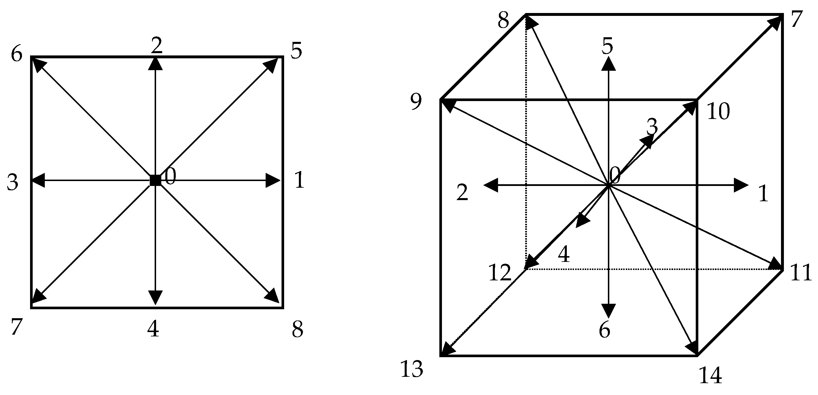
Symmetric lattice velocity directions are adopted in TLBM. The lattice velocity model is named as DaQb, where a and b stand for the dimension and the number of lattice velocity directions, respectively. In the present work, typical D2Q9 model and D3Q15 model (see Figure 1) are applied in two-dimensional and three-dimensional simulations, respectively.

Chapman–Enskog (C-E) expansion analysis is a multi-scale expansion method which is capable to link TLBM to macroscopic governing equations. It can be proven that [14,15], to the second-order of accuracy both in time and in space, Equations (1) and (2) are equivalent to the following macroscopic expressions:

$$\frac{\partial \rho }{\partial t}+\nabla \cdot \left({\displaystyle \sum _{\alpha }{e}_{\alpha }{f}_{\alpha }^{eq}}\right)=0$$

(8)

$$\frac{\partial \rho u}{\partial t}+\nabla \cdot \mathsf{\Pi }=0$$

(9)

$$\frac{\partial \rho e}{\partial t}+\nabla \cdot Q=0$$

(10)

where Π and Q are the momentum flux tensor and the thermal flux vector in the following form

$${\Pi }_{\beta \gamma }={\displaystyle \sum _{\alpha }{\left(e_{\alpha }\right)}_{\beta }{\left(e_{\alpha }\right)}_{\gamma }\left[f_{\alpha }^{eq}+\left(1-\frac{1}{2{\tau }_{\upsilon }}\right)f_{\alpha }^{neq}\right]}$$

(11)

$$Q={\displaystyle \sum _{\alpha }{e}_{\alpha }\left[g_{\alpha }^{eq}+\left(1-\frac{1}{2{\tau }_c}\right)g_{\alpha }^{neq}\right]}$$

(12)

where the non-equilibrium distribution functions have the expressions of

$$f_{\alpha }^{neq}=f_{\alpha }-f_{\alpha }^{eq}=-\tau {\delta }_t\mathrm{D}{f}_{\alpha }^{eq}$$

(13)

$$g_{\alpha }^{neq}=g_{\alpha }-g_{\alpha }^{eq}=-\tau {\delta }_t\mathrm{D}{g}_{\alpha }^{eq}$$

(14)

The single relaxation parameters are related to kinematic viscosity and thermal diffusivity by

$$\upsilon =c_s^2{\delta }_t\left({\tau }_{\upsilon }-\frac{1}{2}\right)$$

(15)

$$\chi =\frac{5}{3}{c}^2{\delta }_t\left({\tau }_c-\frac{1}{2}\right)$$

(16)

2.2. Simplified Thermal Lattice Boltzmann Method (STLBM)

The simplified thermal lattice Boltzmann method (STLBM) is a novel method that is recently developed within LBM framework [12]. Its derivation starts from the macroscopic governing equations recovered from TLBM, i.e., Equations (8)–(10). Assisted by fractional step technique, these equations can be resolved in a predictor–corrector scheme

Predictor step: 

$$\frac{\partial \rho }{\partial t}+\nabla \cdot \left({\displaystyle \sum _{\alpha }{e}_{\alpha }{f}_{\alpha }^{eq}}\right)=0$$

(17)

$$\frac{\partial \rho u}{\partial t}+\nabla \cdot \left[{\displaystyle \sum _{\alpha }{\left(e_{\alpha }\right)}_{\beta }{\left(e_{\alpha }\right)}_{\gamma }{f}_{\alpha }^{eq}}+\frac{1}{2{\tau }_{\upsilon }}{\displaystyle \sum _{\alpha }{\left(e_{\alpha }\right)}_{\beta }{\left(e_{\alpha }\right)}_{\gamma }{f}_{\alpha }^{neq}}\right]=0$$

(18)

$$\frac{\partial \rho e}{\partial t}+\nabla \cdot \left[{\displaystyle \sum _{\alpha }{e}_{\alpha }{g}_{\alpha }^{eq}}+\frac{1}{2{\tau }_c}{\displaystyle \sum _{\alpha }{e}_{\alpha }{g}_{\alpha }^{neq}}\right]=0$$

(19)

Corrector step: 

$$\frac{\partial \rho }{\partial t}=0$$

(20)

$$\frac{\partial \rho u}{\partial t}+\nabla \cdot \left[\left(1-\frac{1}{{\tau }_{\upsilon }}\right){\displaystyle \sum _{\alpha }{\left(e_{\alpha }\right)}_{\beta }{\left(e_{\alpha }\right)}_{\gamma }{f}_{\alpha }^{neq}}\right]-F_E=0$$

(21)

$$\frac{\partial \rho e}{\partial t}+\nabla \cdot \left[\left(1-\frac{1}{{\tau }_c}\right){\displaystyle \sum _{\alpha }{e}_{\alpha }{g}_{\alpha }^{neq}}\right]=0$$

(22)

According to the Boussinesq approximation [16], the external force term can be regarded as a buoyance force related to the temperature profile, i.e.,

$$F_E=\left(\begin{array}{c}0\\ 0\\ -\rho g\beta \left(T-T_m\right)\end{array}\right)$$

(23)

where g is the gravitational acceleration; β is the thermal expansion coefficient; and T_m is the average temperature.

By using lattice properties and the relationships given by C-E analysis, the above Equations (17)–(21) can be reconstructed within the LBM framework to obtain the formulations of simplified thermal lattice Boltzmann method (STLBM)

Predictor step: 

$${\rho }^{\ast }={\displaystyle \sum _{\alpha }{f}_{\alpha }^{eq}\left(r-e_{\alpha }{\delta }_t,t-{\delta }_t\right)}$$

(24)

$${\rho }^{\ast }{u}^{\ast }={\displaystyle \sum _{\alpha }{e}_{\alpha }{f}_{\alpha }^{eq}\left(r-e_{\alpha }{\delta }_t,t-{\delta }_t\right)}$$

(25)

$${\rho }^{\ast }{e}^{\ast }={\displaystyle \sum _{\alpha }{g}_{\alpha }^{eq}\left(r-e_{\alpha }{\delta }_t,t-{\delta }_t\right)}$$

(26)

Corrector step: 

$$\rho \left(r,t\right)={\rho }^{\ast }$$

(27)

$$\rho \left(r,t\right)u\left(r,t\right)={\rho }^{\ast }{u}^{\ast }+\left(1-\frac{1}{{\tau }_{\upsilon }}\right){\displaystyle \sum _{\alpha }{e}_{\alpha }{f}_{\alpha }^{neq}\left(r-e_{\alpha }{\delta }_t,t\right)}+F_E{\delta }_t$$

(28)

$$\rho \left(r,t\right)e\left(r,t\right)={\rho }^{\ast }{e}^{\ast }+\left(1-\frac{1}{{\tau }_c}\right){\displaystyle \sum _{\alpha }{g}_{\alpha }^{neq}\left(r-e_{\alpha }{\delta }_t,t\right)}$$

(29)

Inspired by the treatment in lattice Boltzmann flux solver (LBFS), the non-equilibrium terms involved in Equations (28) and (29) are approximated by the difference between two equilibrium distribution functions at different locations and time levels, i.e.,

$$f_{\alpha }^{neq}\left(r,t\right)=-{\tau }_{\upsilon }{\delta }_t\mathrm{D}{f}_{\alpha }^{eq}\left(r,t\right)=-{\tau }_{\upsilon }\left[f_{\alpha }^{eq}\left(r,t\right)-f_{\alpha }^{eq}\left(r-e_{\alpha }{\delta }_t,t-{\delta }_t\right)\right]$$

(30)

$$g_{\alpha }^{neq}\left(r,t\right)=-{\tau }_c{\delta }_t\mathrm{D}{g}_{\alpha }^{eq}\left(r,t\right)=-{\tau }_c\left[g_{\alpha }^{eq}\left(r,t\right)-g_{\alpha }^{eq}\left(r-e_{\alpha }{\delta }_t,t-{\delta }_t\right)\right]$$

(31)

According to Shu et al. [17] and Wang et al. [18], the equilibrium distribution functions at time level of t is evaluated from the intermediate macroscopic variables obtained in the predictor step.

Compared to the standard TLBM, simplified thermal lattice Boltzmann method (STLBM) possesses many advantages. Although it is developed within LBM framework, STLBM directly updates macroscopic variables instead of the distribution functions. In this way, much fewer virtual memories are required in the computation, and physical boundary conditions can be directly and flexibly implemented without transforming into conditions for the distribution functions. Moreover, by performing von Neumann stability analysis, STLBM can be theoretically proven to be unconditionally stable, which makes it suitable for computations at high Reynolds/Rayleigh numbers.

Despite of the above merits, a serious flaw in STLBM theory is its accuracy. By performing Taylor-series expansion analysis and conservation laws, it can be proven that Equations (24)–(26) in the predictor step can recover corresponding macroscopic Equations (17)–(19) with the second-order of accuracy both in time and in space. However, in the corrector step, it can be shown that when recovering macroscopic Equations (21) and (22), Equations (28) and (29) maintain the second-order of accuracy in space, but present a Euler scheme in time marching, which is only in the first-order of accuracy (see [12] for detail). Since, in LBM framework, the time interval and the mesh spacing are tied up, low order of accuracy in time may have intrinsic effect on overall accuracy of numerical solution.

3. Unconditionally Stable Thermal Lattice Boltzmann Method (USTLBM)

3.1. Modifications on STLBM

The initial formulations in the corrector step are shown in Equations (27)–(29). Apparently, Equation (27) recovers Equation (20) exactly. In the present work, Equations (28) and (29) are, respectively, replaced by the following formulas

$$\rho \left(r,t\right)u\left(r,t\right)={\rho }^{\ast }{u}^{\ast }-\left(1-\frac{1}{{\tau }_{\upsilon }}\right){\displaystyle \sum _{\alpha }{e}_{\alpha }\left[f_{\alpha }^{neq}\left(r+0.5e_{\alpha }{\delta }_t,t-0.5{\delta }_t\right)-f_{\alpha }^{neq}\left(r-0.5e_{\alpha }{\delta }_t,t-0.5{\delta }_t\right)\right]}+F_E{\delta }_t$$

(32)

$$\rho \left(r,t\right)e\left(r,t\right)={\rho }^{\ast }{e}^{\ast }-\left(1-\frac{1}{{\tau }_c}\right){\displaystyle \sum _{\alpha }\left[g_{\alpha }^{neq}\left(r+0.5e_{\alpha }{\delta }_t,t-0.5{\delta }_t\right)-g_{\alpha }^{neq}\left(r-0.5e_{\alpha }{\delta }_t,t-0.5{\delta }_t\right)\right]}$$

(33)

To present theoretical analysis on the accuracy, we start from non-equilibrium distribution functions involved in the above formulations. Performing Taylor-series expansion analysis on Equation (30) with third-order of truncated error gives

$$\begin{array}{l}-{\tau }_{\upsilon }\left[f_{\alpha }^{eq}(\mathit{r},t)-f_{\alpha }^{eq}\left(r-e_{\alpha }{\delta }_t,t-{\delta }_t\right)\right]=-{\tau }_{\upsilon }{\delta }_t\mathrm{D}{f}_{\alpha }^{eq}\left(r-\frac{1}{2}{e}_{\alpha }{\delta }_t,t-\frac{1}{2}{\delta }_t\right)+O\left({\delta }_t^3\right)\\ \hspace{0.17em}\hspace{0.17em}\hspace{0.17em}\hspace{0.17em}\hspace{0.17em}\hspace{0.17em}\hspace{0.17em}\hspace{0.17em}\hspace{0.17em}\hspace{0.17em}\hspace{0.17em}\hspace{0.17em}\hspace{0.17em}\hspace{0.17em}\hspace{0.17em}\hspace{0.17em}\hspace{0.17em}\hspace{0.17em}\hspace{0.17em}\hspace{0.17em}\hspace{0.17em}\hspace{0.17em}\hspace{0.17em}\hspace{0.17em}\hspace{0.17em}\hspace{0.17em}\hspace{0.17em}\hspace{0.17em}\hspace{0.17em}\hspace{0.17em}\hspace{0.17em}\hspace{0.17em}\hspace{0.17em}\hspace{0.17em}\hspace{0.17em}\hspace{0.17em}\hspace{0.17em}\hspace{0.17em}\hspace{0.17em}\hspace{0.17em}\hspace{0.17em}\hspace{0.17em}\hspace{0.17em}\hspace{0.17em}\hspace{0.17em}\hspace{0.17em}=f_{\alpha }^{neq}\left(r-\frac{1}{2}{e}_{\alpha }{\delta }_t,t-\frac{1}{2}{\delta }_t\right)+O\left({\delta }_t^3\right)\end{array}$$

(34)

Similarly, we have

$$g_{\alpha }^{neq}\left(r-\frac{1}{2}{e}_{\alpha }{\delta }_t,t-\frac{1}{2}{\delta }_t\right)=-{\tau }_c\left[g_{\alpha }^{eq}(\mathit{r},t)-g_{\alpha }^{eq}\left(r-e_{\alpha }{\delta }_t,t-{\delta }_t\right)\right]+O\left({\delta }_t^3\right)$$

(35)

Equations (34) and (35) indicate that, with desired order of accuracy, the approximated non-equilibrium distribution functions in Equations (30) and (31) are at space/time level of (r − 0.5e_αδ_t, t − 0.5δ_t). Such shifting in time and space favors our construction of a central-difference scheme both in space and in time, with which the second-order of accuracy can be guaranteed. Maintaining its location in time level, we further expand Equation (34) with respect to the space/time levels of (r, t − 0.5δ_t), which gives

$$\begin{array}{l}{f}_{\alpha }^{neq}\left(r-\frac{1}{2}{e}_{\alpha }{\delta }_t,t-\frac{1}{2}{\delta }_t\right)=f_{\alpha }^{neq}\left(r,t-\frac{1}{2}{\delta }_t\right)-\frac{1}{2}{\delta }_t{e}_{\alpha }\cdot \nabla f_{\alpha }^{neq}\left(r,t-\frac{1}{2}{\delta }_t\right)\\ \hspace{0.17em}\hspace{0.17em}\hspace{0.17em}\hspace{0.17em}\hspace{0.17em}\hspace{0.17em}\hspace{0.17em}\hspace{0.17em}\hspace{0.17em}\hspace{0.17em}\hspace{0.17em}\hspace{0.17em}\hspace{0.17em}\hspace{0.17em}\hspace{0.17em}\hspace{0.17em}\hspace{0.17em}\hspace{0.17em}\hspace{0.17em}\hspace{0.17em}\hspace{0.17em}\hspace{0.17em}\hspace{0.17em}\hspace{0.17em}\hspace{0.17em}\hspace{0.17em}\hspace{0.17em}\hspace{0.17em}\hspace{0.17em}\hspace{0.17em}\hspace{0.17em}\hspace{0.17em}\hspace{0.17em}\hspace{0.17em}\hspace{0.17em}\hspace{0.17em}\hspace{0.17em}+\frac{1}{2}{\left(\frac{1}{2}{\delta }_t\right)}^2{\left[e_{\alpha }\cdot \nabla f_{\alpha }^{neq}\left(r,t-\frac{1}{2}{\delta }_t\right)\right]}^2+O\left({\delta }_t^3\right)\end{array}$$

(36)

$$\begin{array}{l}{f}_{\alpha }^{neq}\left(r+\frac{1}{2}{e}_{\alpha }{\delta }_t,t-\frac{1}{2}{\delta }_t\right)=f_{\alpha }^{neq}\left(r,t-\frac{1}{2}{\delta }_t\right)+\frac{1}{2}{\delta }_t{e}_{\alpha }\cdot \nabla f_{\alpha }^{neq}\left(r,t-\frac{1}{2}{\delta }_t\right)\\ \hspace{0.17em}\hspace{0.17em}\hspace{0.17em}\hspace{0.17em}\hspace{0.17em}\hspace{0.17em}\hspace{0.17em}\hspace{0.17em}\hspace{0.17em}\hspace{0.17em}\hspace{0.17em}\hspace{0.17em}\hspace{0.17em}\hspace{0.17em}\hspace{0.17em}\hspace{0.17em}\hspace{0.17em}\hspace{0.17em}\hspace{0.17em}\hspace{0.17em}\hspace{0.17em}\hspace{0.17em}\hspace{0.17em}\hspace{0.17em}\hspace{0.17em}\hspace{0.17em}\hspace{0.17em}\hspace{0.17em}\hspace{0.17em}\hspace{0.17em}\hspace{0.17em}\hspace{0.17em}\hspace{0.17em}\hspace{0.17em}\hspace{0.17em}\hspace{0.17em}+\frac{1}{2}{\left(\frac{1}{2}{\delta }_t\right)}^2{\left[e_{\alpha }\cdot \nabla f_{\alpha }^{neq}\left(r,t-\frac{1}{2}{\delta }_t\right)\right]}^2+O\left({\delta }_t^3\right)\end{array}$$

(37)

Substituting Equations (36) and (37) into Equation (32) leads to

$$\begin{array}{l}\frac{\rho \left(r,t\right)u\left(r,t\right)-{\rho }^{\ast }{u}^{\ast }}{{\delta }_t}=-\left(1-\frac{1}{{\tau }_{\upsilon }}\right)\frac{1}{{\delta }_t}{\displaystyle \sum _{\alpha }{e}_{\alpha }\left[f_{\alpha }^{neq}\left(r+\frac{1}{2}{e}_{\alpha }{\delta }_t,t-\frac{1}{2}{\delta }_t\right)-f_{\alpha }^{neq}\left(r-\frac{1}{2}{e}_{\alpha }{\delta }_t,t-\frac{1}{2}{\delta }_t\right)\right]}+F_E\\ \hspace{0.17em}\hspace{0.17em}\hspace{0.17em}\hspace{0.17em}\hspace{0.17em}\hspace{0.17em}\hspace{0.17em}\hspace{0.17em}\hspace{0.17em}\hspace{0.17em}\hspace{0.17em}\hspace{0.17em}\hspace{0.17em}\hspace{0.17em}\hspace{0.17em}\hspace{0.17em}\hspace{0.17em}\hspace{0.17em}=-\left(1-\frac{1}{{\tau }_{\upsilon }}\right)\frac{1}{{\delta }_t}{\displaystyle \sum _{\alpha }\left[{\delta }_t{\left(e_{\alpha }\right)}_{\beta }{\left(e_{\alpha }\right)}_{\gamma }\nabla f_{\alpha }^{neq}\left(r,t-\frac{1}{2}{\delta }_t\right)+O\left({\delta }_t^3\right)\right]}+F_E\\ \hspace{0.17em}\hspace{0.17em}\hspace{0.17em}\hspace{0.17em}\hspace{0.17em}\hspace{0.17em}\hspace{0.17em}\hspace{0.17em}\hspace{0.17em}\hspace{0.17em}\hspace{0.17em}\hspace{0.17em}\hspace{0.17em}\hspace{0.17em}\hspace{0.17em}\hspace{0.17em}\hspace{0.17em}\hspace{0.17em}=-\nabla \cdot \left[\left(1-\frac{1}{{\tau }_{\upsilon }}\right){\displaystyle \sum _{\alpha }{\left(e_{\alpha }\right)}_{\beta }{\left(e_{\alpha }\right)}_{\gamma }{f}_{\alpha }^{neq}\left(r,t-\frac{1}{2}{\delta }_t\right)}\right]+O\left({\delta }_t^2\right)+F_E\end{array}$$

(38)

Apparently, the first two terms on right hand side of Equation (38) represent the approximation of the space derivative term in Equation (21) with the second-order of accuracy in space. Meanwhile, the approximated space derivatives are defined at the time level of (t − 0.5δ_t), which represents a typical central difference scheme that ensures the second-order of accuracy in time marching. Through similar processes, it can also be proven that Equation (33) recovers Equation (22) with the second-order of accuracy both in time and in space.

3.2. Unconditionally Stable Thermal Lattice Boltzmann Method (USTLBM)

With the modifications made on previous simplified thermal lattice Boltzmann method (STLBM), formulations of the present unconditionally stable thermal lattice Boltzmann method (USTLBM) are shown as follows:

Predictor step: 

$${\rho }^{\ast }={\displaystyle \sum _{\alpha }{f}_{\alpha }^{eq}\left(r-e_{\alpha }{\delta }_t,t-{\delta }_t\right)}$$

(39)

$${\rho }^{\ast }{u}^{\ast }={\displaystyle \sum _{\alpha }{e}_{\alpha }{f}_{\alpha }^{eq}\left(r-e_{\alpha }{\delta }_t,t-{\delta }_t\right)}$$

(40)

$${\rho }^{\ast }{e}^{\ast }={\displaystyle \sum _{\alpha }{g}_{\alpha }^{eq}\left(r-e_{\alpha }{\delta }_t,t-{\delta }_t\right)}$$

(41)

Corrector step: 

$$\rho \left(r,t\right)={\rho }^{\ast }$$

(42)

$$\rho \left(r,t\right)u\left(r,t\right)={\rho }^{\ast }{u}^{\ast }-\left(1-\frac{1}{{\tau }_{\upsilon }}\right){\displaystyle \sum _{\alpha }{e}_{\alpha }\left[f_{\alpha }^{neq}\left(r+\frac{1}{2}{e}_{\alpha }{\delta }_t,t-\frac{1}{2}{\delta }_t\right)-f_{\alpha }^{neq}\left(r-\frac{1}{2}{e}_{\alpha }{\delta }_t,t-\frac{1}{2}{\delta }_t\right)\right]}+F_E{\delta }_t$$

(43)

$$\rho \left(r,t\right)e\left(r,t\right)={\rho }^{\ast }{e}^{\ast }-\left(1-\frac{1}{{\tau }_c}\right){\displaystyle \sum _{\alpha }\left[g_{\alpha }^{neq}\left(r+\frac{1}{2}{e}_{\alpha }{\delta }_t,t-\frac{1}{2}{\delta }_t\right)-g_{\alpha }^{neq}\left(r-\frac{1}{2}{e}_{\alpha }{\delta }_t,t-\frac{1}{2}{\delta }_t\right)\right]}$$

(44)

where the non-equilibrium terms are evaluated by

$$f_{\alpha }^{neq}\left(r-\frac{1}{2}{e}_{\alpha }{\delta }_t,t-\frac{1}{2}{\delta }_t\right)=-{\tau }_{\upsilon }\left[f_{\alpha }^{eq}(\mathit{r},t)-f_{\alpha }^{eq}\left(r-e_{\alpha }{\delta }_t,t-{\delta }_t\right)\right]$$

(45)

$$g_{\alpha }^{neq}\left(r-\frac{1}{2}{e}_{\alpha }{\delta }_t,t-\frac{1}{2}{\delta }_t\right)=-{\tau }_c\left[g_{\alpha }^{eq}(\mathit{r},t)-g_{\alpha }^{eq}\left(r-e_{\alpha }{\delta }_t,t-{\delta }_t\right)\right]$$

(46)

To ensure the second-order of accuracy in time, the external force term F_E should be defined on (r, t − 0.5δ_t). According to Boussinesq approximation shown in Equation (23), this term is approximated by

$$F_{Ex}=0,\hspace{0.17em}\hspace{0.17em}{F}_{Ey}=0,\hspace{0.17em}\hspace{0.17em}{F}_{Ez}=-0.5\rho g\beta \left[T\left(r,t\right)+T\left(r,t-{\delta }_t\right)-2T_m\right]$$

(47)

Since T(r,t) can be solved firstly and then substituted into Equation (47) in the same time step, the equations are decoupled and the explicitness of the scheme is ensured.

As discussed above, USTLBM is an improved version of STLBM and is a truly second-order method. Nevertheless, the basic idea of USTLBM is similar to that of STLBM, which is to reconstruct solutions to macroscopic governing equations within LBM framework. Such characteristics grant USTLBM advantages from both STLBM and standard LBM. On one hand, USTLBM maintains the simplicity and explicitness, and ensures the second-order of accuracy in time and space as standard LBM does. On the other hand, USTLBM directly updates macroscopic variables rather than distribution functions, which greatly lowers virtual memories and facilitates implementation of physical boundary conditions. Moreover, as its name indicates, USTLBM can be theoretically proven to be unconditionally stable, which will be discussed in detail in following sections.

3.3. Boundary Conditions

In its computational process, USTLBM calls for boundary values of both macroscopic variables and non-equilibrium distribution functions. The physical boundary condition, which is related to macroscopic variables, can be directly implemented. Specifically, Dirichlet boundary condition can be imposed by artificially assigning boundary values of macroscopic variables on boundary meshes; and Neumann boundary condition can be fulfilled by adopting information on several inner layers of meshes to achieve desired order of accuracy.

Boundary values of non-equilibrium distribution functions are required in the corrector step of USTLBM, as shown in Equations (43) and (44). It has been proven in previous studies that the non-equilibrium extrapolation scheme can ensure the second order of accuracy in space [17]. In this treatment, the boundary values of non-equilibrium distribution functions are set equal to those on the first inner layer of mesh points. Such boundary treatment can be flexibly applied in uniform and non-uniform meshes, and will be used in the present method in determining boundary values of non-equilibrium terms.

3.4. Stability Analysis

Theoretical analysis for the stability of lattice Boltzmann method (LBM) was firstly conducted by Sterling and Chen [18]. It was found that standard LBM suffers from numerical instability when the single relaxation parameter τ is close to 0.5, which indicates that standard LBM is not suitable to problems at high Reynolds numbers. The recently developed simplified thermal lattice Boltzmann method (STLBM), on the other hand, performs very well in numerical stability. Through von Neumann stability analysis, it can be proven that STLBM is unconditionally stable [12]. The USTLBM proposed in this paper can be regarded as an improved version of STLBM that ensures higher order of accuracy in time. In this section, we use von Neumann stability analysis to study its stability performance. For the ease of analysis, we take the two-dimensional formulations as the example here. Analysis on the three-dimensional formulations can be carried out through similar processes, and same conclusions can be obtained.

To begin with, the following macroscopic variables are defined:

$$y_1=\rho ,\hspace{0.17em}\hspace{0.17em}\hspace{0.17em}{y}_2=\rho u,\hspace{0.17em}\hspace{0.17em}\hspace{0.17em}{y}_3=\rho v,\hspace{0.17em}\hspace{0.17em}\hspace{0.17em}{y}_4=\rho e$$

(48)

The vector of these variables is then written as

$$Y={\left(\begin{array}{cccc}{y}_1& y_2& y_3& y_4\end{array}\right)}^{\mathrm{T}}$$

(49)

The equilibrium distribution functions Equations (3) and (4) are functions of the macroscopic variables, which can be written as

$$f_{\alpha }^{eq}=w_{\alpha }{y}_{1\alpha }+\frac{w_{\alpha }}{c_s^2}\left(e_{\alpha x}{y}_{2\alpha }+e_{\alpha y}{y}_{3\alpha }\right)+\frac{w_{\alpha }}{2c_s^4}\frac{{\left(e_{\alpha x}{y}_{2\alpha }+e_{\alpha y}{y}_{3\alpha }\right)}^2}{y_{1\alpha }}-\frac{w_{\alpha }}{2c_s^2}\frac{y_{2\alpha }^2+y_{3\alpha }^2}{y_{1\alpha }}$$

(50)

$$g_{\alpha }^{eq}=\{\begin{array}{l}-\frac{2}{3}{y}_{4\alpha }\frac{y_{2\alpha }^2+y_{3\alpha }^2}{y_{1\alpha }^2}\hspace{0.17em}\hspace{0.17em}\hspace{0.17em}\hspace{0.17em}\hspace{0.17em}\hspace{0.17em}\hspace{0.17em}\hspace{0.17em}\hspace{0.17em}\hspace{0.17em}\hspace{0.17em}\hspace{0.17em}\hspace{0.17em}\hspace{0.17em}\hspace{0.17em}\hspace{0.17em}\hspace{0.17em}\hspace{0.17em}\hspace{0.17em}\hspace{0.17em}\hspace{0.17em}\hspace{0.17em}\hspace{0.17em}\hspace{0.17em}\hspace{0.17em}\hspace{0.17em}\hspace{0.17em}\hspace{0.17em}\hspace{0.17em}\hspace{0.17em}\hspace{0.17em}\hspace{0.17em}\hspace{0.17em}\hspace{0.17em}\hspace{0.17em}\hspace{0.17em}\hspace{0.17em}\hspace{0.17em}\hspace{0.17em}\hspace{0.17em}\hspace{0.17em}\hspace{0.17em}\hspace{0.17em}\hspace{0.17em}\hspace{0.17em}\hspace{0.17em}\hspace{0.17em}\hspace{0.17em}\hspace{0.17em}\hspace{0.17em}\hspace{0.17em}\hspace{0.17em}\hspace{0.17em}\hspace{0.17em}\hspace{0.17em}\hspace{0.17em}\hspace{0.17em}\hspace{0.17em}\hspace{0.17em}\hspace{0.17em}\hspace{0.17em}\hspace{0.17em}\hspace{0.17em}\hspace{0.17em}\hspace{0.17em}\hspace{0.17em}\hspace{0.17em}\alpha =0\\ \frac{1}{6}{y}_{4\alpha }+\frac{1}{6}{y}_{4\alpha }\frac{e_{\alpha x}{y}_{2\alpha }+e_{\alpha y}{y}_{3\alpha }}{y_{1\alpha }}+\frac{1}{2}{y}_{4\alpha }{\left(\frac{e_{\alpha x}{y}_{2\alpha }+e_{\alpha y}{y}_{3\alpha }}{y_{1\alpha }}\right)}^2-\frac{1}{6}{y}_{4\alpha }\frac{y_{2\alpha }^2+y_{3\alpha }^2}{y_{1\alpha }^2}\hspace{0.17em}\hspace{0.17em}\hspace{0.17em}\hspace{0.17em}\hspace{0.17em}\alpha =1~4\\ \frac{1}{12}{y}_{4\alpha }+\frac{1}{6}{y}_{4\alpha }\frac{e_{\alpha x}{y}_{2\alpha }+e_{\alpha y}{y}_{3\alpha }}{y_{1\alpha }}+\frac{1}{8}{y}_{4\alpha }{\left(\frac{e_{\alpha x}{y}_{2\alpha }+e_{\alpha y}{y}_{3\alpha }}{y_{1\alpha }}\right)}^2-\frac{1}{24}{y}_{4\alpha }\frac{y_{2\alpha }^2+y_{3\alpha }^2}{y_{1\alpha }^2}\hspace{0.17em}\hspace{0.17em}\hspace{0.17em}\alpha =5~8\end{array}$$

(51)

where y_1α, y_2α, y_3α and y_4α denote the functional values of y₁, y₂, y₃ and y₄ at the space/time level of (r-e_α, t-δ_t), respectively. Substituting Equations (50) and (51) into the expressions for the intermediate density, momentum and energy (Equations (39)–(41)) gives a set of nonlinear algebraic equations Y^* = F(Yⁿ). To linearize the problem to perform von Neumann stability analysis, the obtained equations are differentiated with respect to y₁, y₂, y₃ and y₄, which leads to

$$\mathrm{d}{Y}^{\ast }={\left[\frac{\partial Y^{\ast }}{\partial y_1}\right]}^n\mathrm{d}{y}_1^n+{\left[\frac{\partial Y^{\ast }}{\partial y_2}\right]}^n\mathrm{d}{y}_2^n+{\left[\frac{\partial Y^{\ast }}{\partial y_3}\right]}^n\mathrm{d}{y}_3^n+{\left[\frac{\partial Y^{\ast }}{\partial y_4}\right]}^n\mathrm{d}{y}_4^n$$

(52)

where Y* = (y₁^*, y₂^*, y₃^*, y₄^*)^T; and the superscript n represents the time level. For illustration purposes, we take the term [∂y₂^*/∂y₂]ⁿ to elaborate the analyzing process:

$${\left[\frac{\partial y_2^{\ast }}{\partial y_2}\right]}^n={\displaystyle \sum _{\alpha }\left[\frac{w_{\alpha }{e}_{\alpha x}^2}{c_s^2}+\frac{w_{\alpha }{e}_{\alpha x}^3{y}_{2\alpha }^n}{c_s^4{y}_{1\alpha }^n}+\frac{w_{\alpha }{e}_{\alpha x}^2{e}_{\alpha y}{y}_{3\alpha }^n}{c_s^4{y}_{1\alpha }^n}-\frac{w_{\alpha }{e}_{\alpha x}{y}_{2\alpha }^n}{c_s^2{y}_{1\alpha }^n}\right]}$$

(53)

In von-Neumann stability analysis, the variables are approximated by the Fourier serial expansions [2]. Consider a random component of the variables encountered here, which can be written as

$$\mathrm{d}{y}_i^{\ast }={\overline{\mathrm{d}y}}_i^{\ast }{e}^{jk\cdot r};\hspace{0.17em}\mathrm{d}{y}_i^n={\overline{\mathrm{d}y}}_i^n{e}^{jk\cdot r};\hspace{0.17em}{y}_{i\alpha }^n=y_i^n{e}^{ik\cdot \left(r-e_{\alpha }{\delta }_t\right)},i=1-4$$

(54)

In addition, note that the following isotropic properties of the lattice tensors are generally applicable within LBM framework:

$$\begin{array}{l}{\displaystyle \sum _{\alpha }{w}_{\alpha }{e}_{\alpha x}^2{e}_{\alpha y}}={\displaystyle \sum _{\alpha }{w}_{\alpha }{e}_{\alpha x}{e}_{\alpha y}^2}={\displaystyle \sum _{\alpha }{w}_{\alpha }{e}_{\alpha x}^3}={\displaystyle \sum _{\alpha }{w}_{\alpha }{e}_{\alpha y}^3}=0\\ {\displaystyle \sum _{\alpha }{w}_{\alpha }{e}_{\alpha x}^2}={\displaystyle \sum _{\alpha }{w}_{\alpha }{e}_{\alpha y}^2}=c_s^2\\ {\displaystyle \sum _{\alpha }{w}_{\alpha }{e}_{\alpha x}{e}_{\alpha y}}=0\\ {\displaystyle \sum _{\alpha }{w}_{\alpha }}=1\\ {\displaystyle \sum _{\alpha }{w}_{\alpha }{e}_{\alpha x}}={\displaystyle \sum _{\alpha }{w}_{\alpha }{e}_{\alpha y}}=0\end{array}$$

(55)

Substituting Equations (54) and (55) into Equation (53), we can derive that

$$\begin{array}{l}{\left[\frac{\partial y_2^{\ast }}{\partial y_2}\right]}^n=\frac{1}{c_s^2}{\displaystyle \sum _{\alpha }{w}_{\alpha }{e}_{\alpha x}^2}+\frac{y_2^n}{c_s^4{y}_1^n}{\displaystyle \sum _{\alpha }{w}_{\alpha }{e}_{\alpha x}^3}+\frac{y_3^n}{c_s^4{y}_1^n}{\displaystyle \sum _{\alpha }{w}_{\alpha }{e}_{\alpha x}^2{e}_{\alpha y}}+\frac{y_2^n}{c_s^2{y}_1^n}{\displaystyle \sum _{\alpha }{w}_{\alpha }{e}_{\alpha x}}\\ \hspace{0.17em}\hspace{0.17em}\hspace{0.17em}\hspace{0.17em}\hspace{0.17em}\hspace{0.17em}\hspace{0.17em}\hspace{0.17em}\hspace{0.17em}\hspace{0.17em}=1\end{array}$$

(56)

Following similar processes shown in Equations (53)–(56), we can find the values of all terms inside the brackets in Equation (52) (i.e., [∂y_i^*/∂y_j]ⁿ); and the equation can be simplified as

$${\overline{\mathrm{d}Y}}^{\ast }={\overline{\mathrm{d}Y}}^n$$

(57)

In the corrector step, it is shown in Equation (42) that no correction is performed on the density. Therefore, we can simply derive that

$${\overline{\mathrm{d}y}}_1^{n+1}={\overline{\mathrm{d}y}}_1^{\ast }={\overline{\mathrm{d}y}}_1^n$$

(58)

Next, we still take the variable y₂ to illustrate the analyzing process in the corrector step. According to Equations (40), (43), and (45), we have

$$y_2^{n+1}=y_2^{\ast }+\left({\tau }_{\upsilon }-1\right){\displaystyle \sum _{\alpha }{e}_{\alpha x}{f}_{\alpha }^{eq}\left(r+e_{\alpha }{\delta }_t,t\right)}-\left({\tau }_{\upsilon }-1\right)y_2^{\ast }$$

(59)

Substitution of the equilibrium distribution based on the intermediate macroscopic variables into the second term on RHS of the above equation gives a nonlinear algebraic formula of

$$\begin{array}{l}S={\displaystyle \sum _{\alpha }{e}_{\alpha x}{f}_{\alpha }^{eq}\left(r+e_{\alpha }{\delta }_t,t\right)}\\ \hspace{0.17em}\hspace{0.17em}\hspace{0.17em}={\displaystyle \sum _{\alpha }{e}_{\alpha x}{w}_{\alpha }{y}_{1-\alpha }^{\ast }}+{\displaystyle \sum _{\alpha }{e}_{\alpha x}\frac{w_{\alpha }}{c_s^2}\left(e_{\alpha x}{y}_{2-\alpha }^{\ast }+e_{\alpha y}{y}_{3-\alpha }^{\ast }\right)}\\ \hspace{0.17em}\hspace{0.17em}\hspace{0.17em}\hspace{0.17em}\hspace{0.17em}+{\displaystyle \sum _{\alpha }{e}_{\alpha x}\frac{w_{\alpha }}{2c_s^4}\frac{{\left(e_{\alpha x}{y}_{2-\alpha }^{\ast }+e_{\alpha y}{y}_{3-\alpha }^{\ast }\right)}^2}{y_{1-\alpha }^{\ast }}}-{\displaystyle \sum _{\alpha }{e}_{\alpha x}\frac{w_{\alpha }}{2c_s^2}\frac{{\left(y_{2-\alpha }^{\ast }\right)}^2+{\left(y_{3-\alpha }^{\ast }\right)}^2}{y_{1-\alpha }^{\ast }}}\end{array}$$

(60)

where the subscript “−α” represents the space level of (r + e_αδ_t). Similar to the procedures conducted in the corrector step, here we linearize the formula by differentiating it, which gives

$$\mathrm{d}S={\left(\frac{\partial S}{\partial y_1}\right)}^{\ast }\mathrm{d}{y}_1^{\ast }+{\left(\frac{\partial S}{\partial y_2}\right)}^{\ast }\mathrm{d}{y}_2^{\ast }+{\left(\frac{\partial S}{\partial y_3}\right)}^{\ast }\mathrm{d}{y}_3^{\ast }$$

(61)

Following similar processes shown in Equations (53)–(56), the values of terms inside brackets can be evaluated. Subsequently, Equation (61) is simplified as

$$\overline{\mathrm{d}S}=\overline{\mathrm{d}{y}_2^{\ast }}$$

(62)

Differentiating Equation (59) and substituting Equations (54) and (62) into it eventually gives

$${\overline{\mathrm{d}y}}_2^{n+1}\hspace{0.17em}={\overline{\mathrm{d}y}}_2^n$$

(63)

Other variables in the corrector step can be analyzed through similar procedures to derive the following relationship:

$$\{\begin{array}{l}{\overline{\mathrm{d}y}}_1^{n+1}\hspace{0.17em}={\overline{\mathrm{d}y}}_1^n\\ {\overline{\mathrm{d}y}}_2^{n+1}\hspace{0.17em}={\overline{\mathrm{d}y}}_2^n\\ {\overline{\mathrm{d}y}}_3^{n+1}=g\beta T_m{\delta }_t{\overline{\mathrm{d}y}}_1^n+{\overline{\mathrm{d}y}}_3^n-g\beta {\delta }_t{\overline{\mathrm{d}y}}_4^n\\ {\overline{\mathrm{d}y}}_4^{n+1}\hspace{0.17em}={\overline{\mathrm{d}y}}_4^n\end{array}$$

(64)

Thus, the overall stability analysis of USTLBM can be written in the matrix form of

$${\overline{\mathrm{d}Y}}^{n+1}=\left[\begin{array}{cccc}1& 0& 0& 0\\ 0& 1& 0& 0\\ g\beta T_m{\delta }_t& 0& 1& -g\beta {\delta }_t\\ 0& 0& 0& 1\end{array}\right]\cdot {\overline{\mathrm{d}Y}}^n$$

(65)

Apparently, all eigenvalues in the characteristic matrix are 1. Therefore, it is proven that USTLBM proposed in this paper is theoretically unconditionally stable.

Through the above von Neumann stability analysis, it turns out that USTLBM maintains the merit of STLBM in numerical stability; therefore, both of them are advantageous over the standard LBM. Meanwhile, considering its advantage in temporal accuracy, USTLBM is more competitive than STLBM in the perspective of numerical accuracy.

3.5. Computational Procedure

The computational sequence of the present unconditionally stable thermal lattice Boltzmann method (USTLBM) can be summarized as follows:

(1)

Specify the streaming distance δ_x (δ_x = δ_t). Determine the single relaxation parameters τ_υ and τ_c according to Equations (15) and (16).

(2)

Predictor step: Use Equations (39)–(41) to calculate the intermediate macroscopic properties ρ^*, u^* and e^*.

(3)

Approximate the non-equilibrium distribution functions (f_α^neq and g_α^neq) by applying Equations (45) and (46).

(4)

Implement non-equilibrium extrapolation scheme to determine boundary values of the non-equilibrium distribution functions.

(5)

Corrector step: Evaluate density, velocity, and internal energy at the new time step from Equations (42)–(44). The external force term F_E is calculated by Equation (47).

(6)

Implement physical boundary conditions for the macroscopic variables.

(7)

Repeat Steps (2)–(6) until the computation converges or the prescribed maximum time step is reached.

4. Numerical Tests

In this part, we present four numerical examples to demonstrate the robustness and the flexibility of USTLBM in modeling incompressible thermal flows. Numerical accuracy and stability are evaluated through typical numerical experiments to validate the theoretical conclusions made in previous sections (i.e., USTLBM ensures the second-order of accuracy in space and is unconditionally stable). Combining with Lagrangian interpolation algorithms, the present method can be flexibly extended to non-uniform meshes and body-fitted meshes to achieve higher efficiency and to study problems with curved boundaries.

4.1. 2D Natural Convection in a Square Cavity

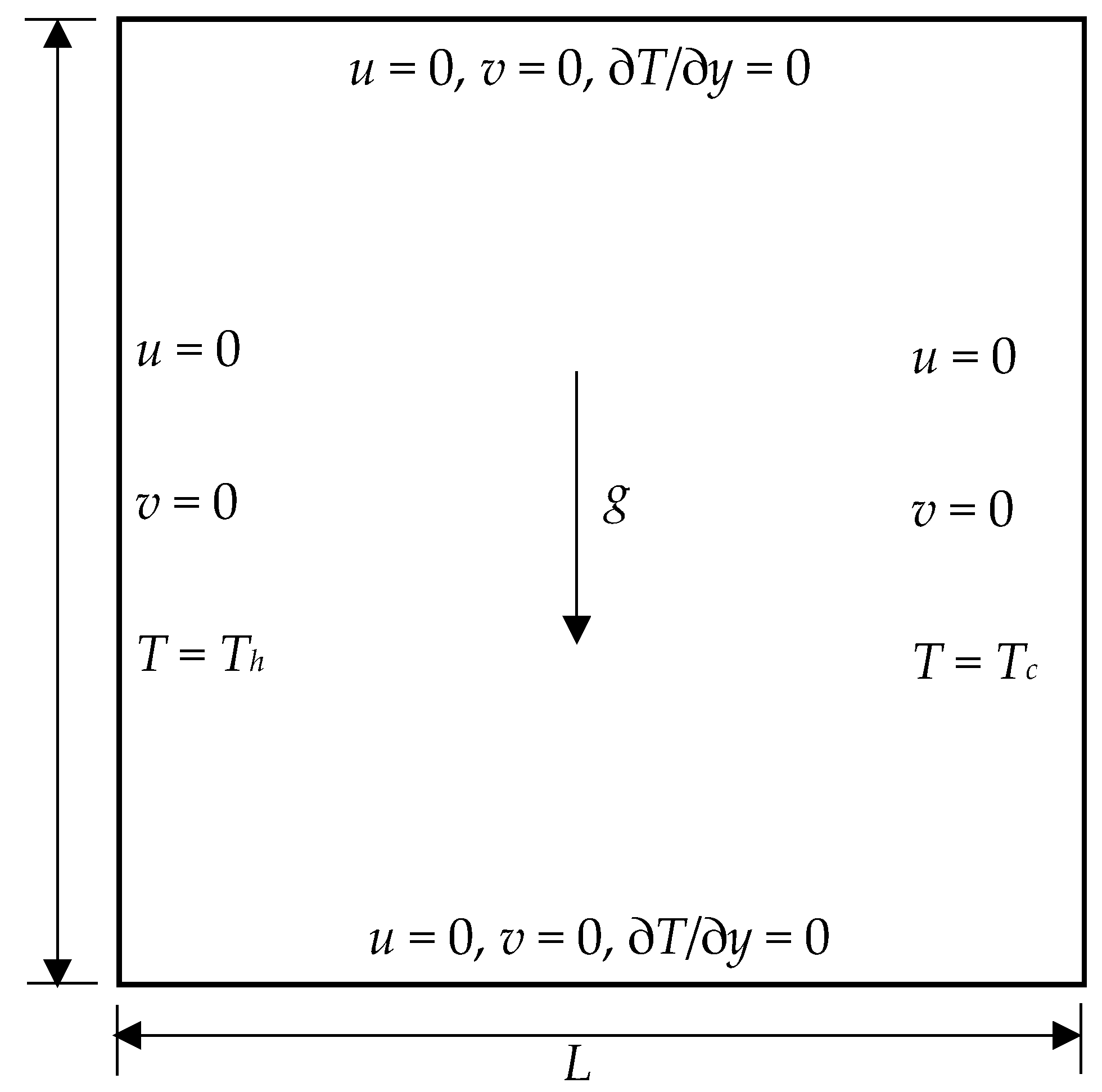
Natural convection in a square cavity is a classic benchmark test to validate numerical methods for thermal flows. In this section, we use the example in two-dimensional scenario to assess accuracy, convergence, and stability performance of USTLBM. Physical configuration of this problem is shown in Figure 2. Key non-dimensional parameters that affect the flow pattern are the Rayleigh number and the Prandtl number defined as

$$Ra=\frac{g\beta \cdot \Delta T\cdot L^3}{\upsilon \cdot \chi }=\frac{V_c^2\cdot L^2}{\upsilon \cdot \chi }$$

(66)

$$Pr=\frac{\upsilon }{\chi }$$

(67)

where ΔT is the temperature difference between the left hot wall and the right cold wall; and V_c is the characteristic velocity defined as $V_c=\sqrt{g\beta L\cdot \Delta T}$. In our simulations, Pr is set to be 0.71, and V_c = 1 to fulfill the low Mach number assumption. Various Nusselt numbers are defined to quantify the heat transfer rate. Specifically, the volume averaged Nusselt number and the average Nusselt number on the hot wall are

$$\overline{Nu}=\frac{L}{\chi \cdot \Delta T}\cdot \frac{1}{L^2}{\displaystyle \underset{\Omega }{\iint }\left(uT-\chi \frac{\partial T}{\partial x}\right)}\mathrm{d}\Omega$$

(68)

$$N{u}_0=\frac{1}{L\cdot \Delta T}{\displaystyle \underset{x=0}{\int }\frac{\partial T}{\partial x}\mathrm{d}y}$$

(69)

Initially, we use the case with Ra = 10⁴ to validate spatial accuracy of USTLBM. Since analytical solution to this problem is unavailable, the benchmark result of the volume averaged Nusselt number obtained by the mesh size of 301 × 301 is used as the reference data ${\overline{Nu}}_a$. Various mesh sizes of 11 × 11, 21 × 21, 41 × 41, 61 × 61 and 81 × 81 are adopted and corresponding relative errors are calculated through the following formula

$$E=\frac{\left|\overline{Nu}-{\overline{Nu}}_a\right|}{\left|{\overline{Nu}}_a\right|}$$

(70)

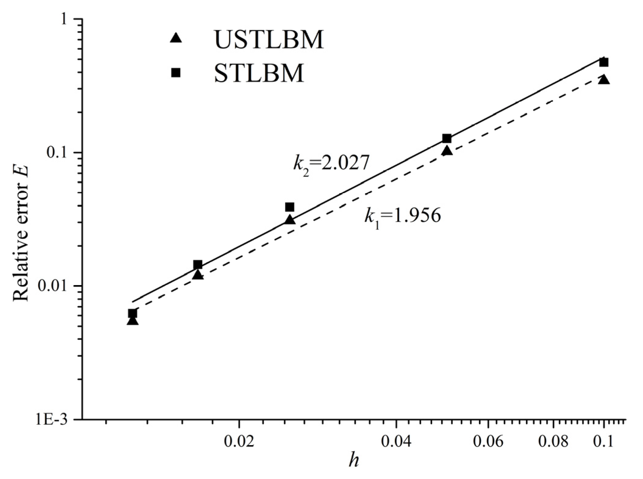
The relative errors obtained at different mesh sizes are depicted in Figure 3. As can be seen, the linearly fitted line of the data reveals a slope of 1.956 in log scale, which indicates that USTLBM can ensure the second-order of accuracy in space. The result obtained by STLBM is also included in this figure. The fitted line of the data given by STLBM also has a slope that is very near to 2.0, which validates that STLBM can ensure the second-order of accuracy in space. However, it should be noted that the order of accuracy and the numerical error (e.g., the relative error to the reference data in this example) are two different concepts. The numerical error is usually written as Error = O(hⁿ) = C·hⁿ, where h is the mesh spacing, n is the order of accuracy, and C is a constant. Clearly, the order of accuracy is the slope of straight line of log (error) vs. log(h). Even if the order of accuracy n is the same, the relative numerical error of one method can still be smaller than that of another method at the same mesh size (i.e., C value of two methods may not be the same). Detailed comparisons show that, at the same mesh spacing, relative error of the results given by USTLBM is lower than that obtained by STLBM. Therefore, it is reasonable to expect more accurate results at the same mesh resolution when applying USTLBM.

More cases in high Rayleigh numbers of Ra = 10⁵, 10⁶, 10⁷ and 10⁸ are simulated by both USTLBM and STLBM with different mesh resolutions. Note that, in cases of Ra = 10⁷ and 10⁸, non-uniform meshes are adopted to capture severe changes of flow fields near boundaries. Lagrange interpolation algorithm is applied to determine functional values on locations where the streaming process initiates. Representative flow parameters are tabulated in

Table 1. Comparisons of flow parameters in Ra = 10⁵ at different mesh sizes.

Parameters	Grid	112	1512	2012	2512	3012	Reference [19,20,21,22]
Nu0	STLBM	1.096	4.503	4.526	4.530	4.531	4.504–4.532
	USTLBM	1.365	4.513	4.527	4.530	4.530
umax	STLBM	36.900	34.531	34.566	34.596	34.624	34.736–34.87
	USTLBM	55.550	34.523	34.577	34.610	34.635
vmax	STLBM	37.166	68.075	68.351	68.456	68.545	68.22–68.85
	USTLBM	56.930	68.200	68.390	68.464	68.552

,

Table 2. Comparisons of flow parameters in Ra = 10⁶ at different mesh sizes.

Parameters	Grid	112	2012	2512	3012	3512	Reference [19,20,21,22]
Nu0	STLBM	1.115	8.434	8.634	8.732	8.782	8.767–8.928
	USTLBM	1.457	8.599	8.724	8.781	8.810
umax	STLBM	122.78	63.665	64.005	64.173	64.364	64.775–65.33
	USTLBM	188.10	64.346	64.441	64.513	64.577
vmax	STLBM	123.73	214.16	217.36	218.56	219.21	216.75–221.19
	USTLBM	193.61	217.64	218.61	219.11	219.65

,

Table 3. Comparisons of flow parameters in Ra = 10⁷ at different mesh sizes.

Parameters	Grid	112	2012	2512	3012	3512	Reference [23,24,25]
Nu1/2	STLBM	95.807	16.272	16.366	16.420	16.449	16.52–16.543
	USTLBM	101.05	16.334	16.407	16.443	16.463
umax	STLBM	548.08	142.81	145.58	146.64	147.21	148.58–148.84
	USTLBM	570.11	144.87	146.53	147.31	147.73
vmax	STLBM	606.26	696.33	698.10	698.74	699.01	699.18–699.91
	USTLBM	635.02	699.30	699.32	699.37	699.40

and

Table 4. Comparisons of flow parameters in Ra = 10⁸ at different mesh sizes.

Parameters	Grid	112	3012	3512	4012	4512	Reference [23,24,25]
Nu1/2	STLBM	305.29	26.737	29.610	29.774	29.875	30.225–30.301
	USTLBM	322.15	29.744	29.874	29.958	30.014
umax	STLBM	1730.3	551.59	294.05	297.02	302.28	321.37–323.65
	USTLBM	1799.6	312.71	317.23	319.76	321.27
vmax	STLBM	1919.2	2503.2	2199.3	2206.7	2212.3	2222.0–2222.9
	USTLBM	2010.4	2219.6	2220.1	2221.6	2222.0

. It is noteworthy that, in all cases, both USTLBM and STLBM do not diverge at very coarse mesh size of 11 × 11, and reasonable results of flow parameters can be achieved. Such performance demonstrates that both USTLBM and STLBM have very good numerical stability, which makes them superior to standard LBM that can easily diverge in cases with high Reynolds/Rayleigh numbers. Convergence study is also carried out with various mesh sizes adopted in these cases. It turns out that the calculated flow parameters are approaching to the reference data by refining the meshes, which verifies that both USTLBM and STLBM can converge to the correct answer.

Another notable issue reflected in these tables is that at the same mesh size, the results obtained by USTLBM show smaller relative errors to the reference data. At high Rayleigh numbers, STLBM usually requires finer meshes to achieve comparable results. Here, we take the maximum vertical velocity for illustration. At Ra = 10⁶, results obtained by USTLBM are within the range given by reference data at the mesh size of 201 × 201, while STLBM can only get comparable results at the mesh size of 251 × 251. In the case of Ra = 10⁸, the relative error of results obtained by USTLBM at the mesh size of 301 × 301 is within 0.02%, while the relative error of STLBM at the same mesh size is 12.66%. These results evidently prove that, although in the same order of accuracy, USTLBM is more accurate than STLBM at the same mesh size.

4.2. Mixed Convection in a Lid-Driven Cavity

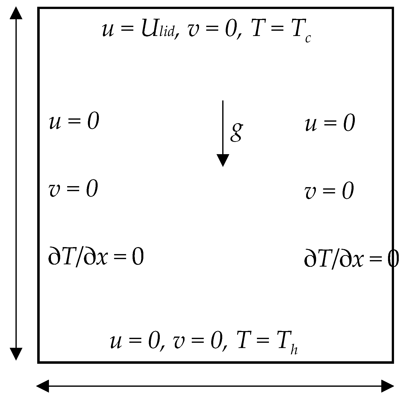
In this section, we present the example of mixed convection in a lid-driven cavity. The physical configuration of the problem is a square cavity with moving top lid and three stationary walls. The top and the bottom walls are maintained at constant cold and hot temperatures (T_c and T_h), respectively (see Figure 4). Neumann boundary condition for the temperature with its normal gradient equal to zero is implemented on the right/left walls. Typical non-dimensional parameters defined for this problem include Reynolds number, Grashof number, Prandtl number and Richardson number, which are expressed as

$$Re=\frac{U_{lid}L}{\upsilon }$$

(71)

$$Gr=\frac{g\beta \left(T_h-T_c\right)L^3}{{\upsilon }^2}$$

(72)

$$Pr=\frac{\upsilon }{\chi }$$

(73)

$$Ri=\frac{Gr}{R{e}^2}$$

(74)

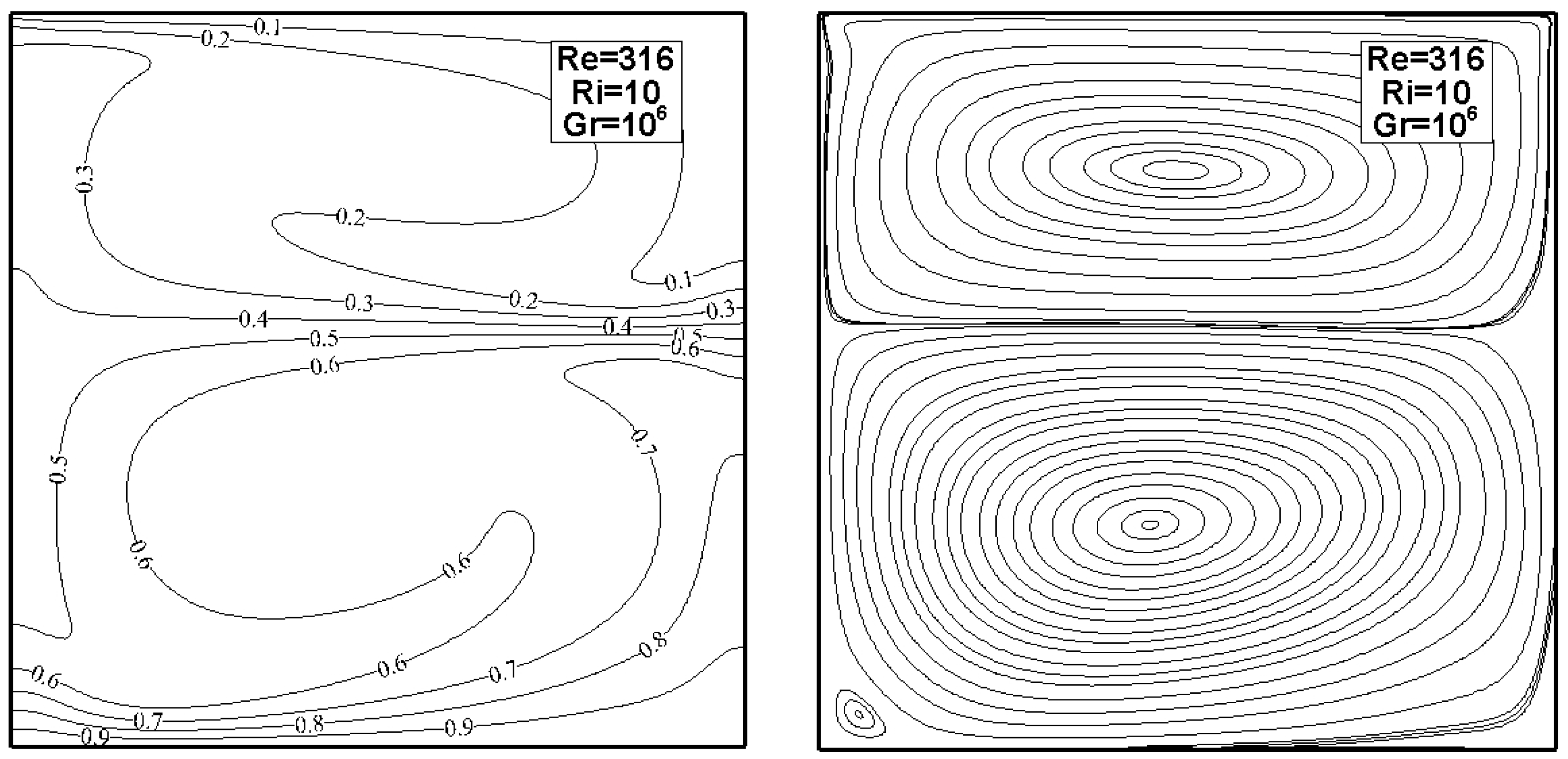
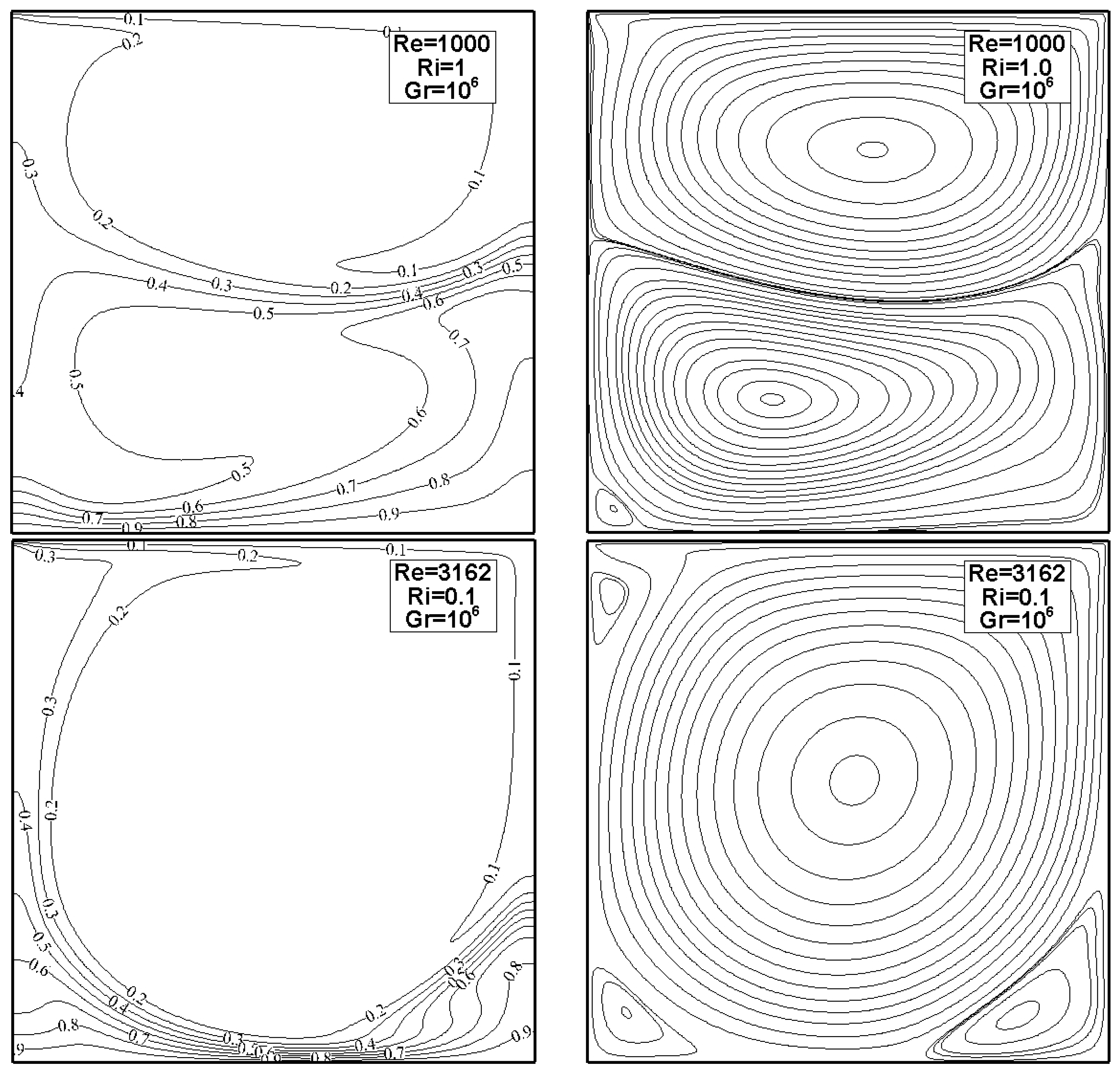
Referring to set-ups in previous studies [26,27], here we set Gr = 10⁶ and Pr = 0.71, and three cases with different Richardson numbers of 10, 1.0 and 0.1 are simulated. Uniform mesh with the size of 251 × 251 is adopted in our simulations.

Figure 5 presents isotherms and streamlines at steady state obtained by USTLBM. As can be seen, smoothness of the isotherms and streamlines is well maintained by the present USTLBM. It is also observed that, at larger Ri number (e.g., Ri = 10), two major vortices show up in the flow pattern. With the decreasing of the Ri number, the lower vortex is gradually compressed. When Ri number is sufficiently small (e.g., Ri = 0.1), only one major vortex exists and the flow pattern is quite similar to the classic lid-driven cavity flow at the same Reynolds number. The physical mechanism of such phenomenon is the relative importance of natural convection to the forced convection, which is the essence of Richardson number. At low Ri number, the effect of the natural convection is quite small or even negligible, due to which the final flow pattern is mainly shaped by the shear force induced by the moving lid. Therefore, the streamlines at low Ri number are very much like those of isothermal lid-driven cavity flows at the same Reynolds number. In high Ri number scenario, natural convection has comparable or even larger effect on the flow field as the forced convection does. Subsequently, the buoyance force induced by the temperature gradient enlarges the vortex on the right corner and eventually makes its size comparable to that of the main vortex.

For quantitative comparison, the average Nusselt numbers on the hot wall at different Richardson numbers are presented in

Table 5. Comparison of average Nusselt number on hot wall for the mixed convection in lid-driven cavity.

Ri	Cheng and Liu [26]	Bettaibi et al. [27]	Present
10	4.860	4.848	4.786
1	5.750	5.739	5.694
0.1	12.161	12.138	12.016

. Apparently, the computational results in our simulations agree well with the reference data in the literature. Therefore, the robustness of USTLBM in this mixed convection problem is validated.

4.3. Natural Convection in a Concentric Annulus

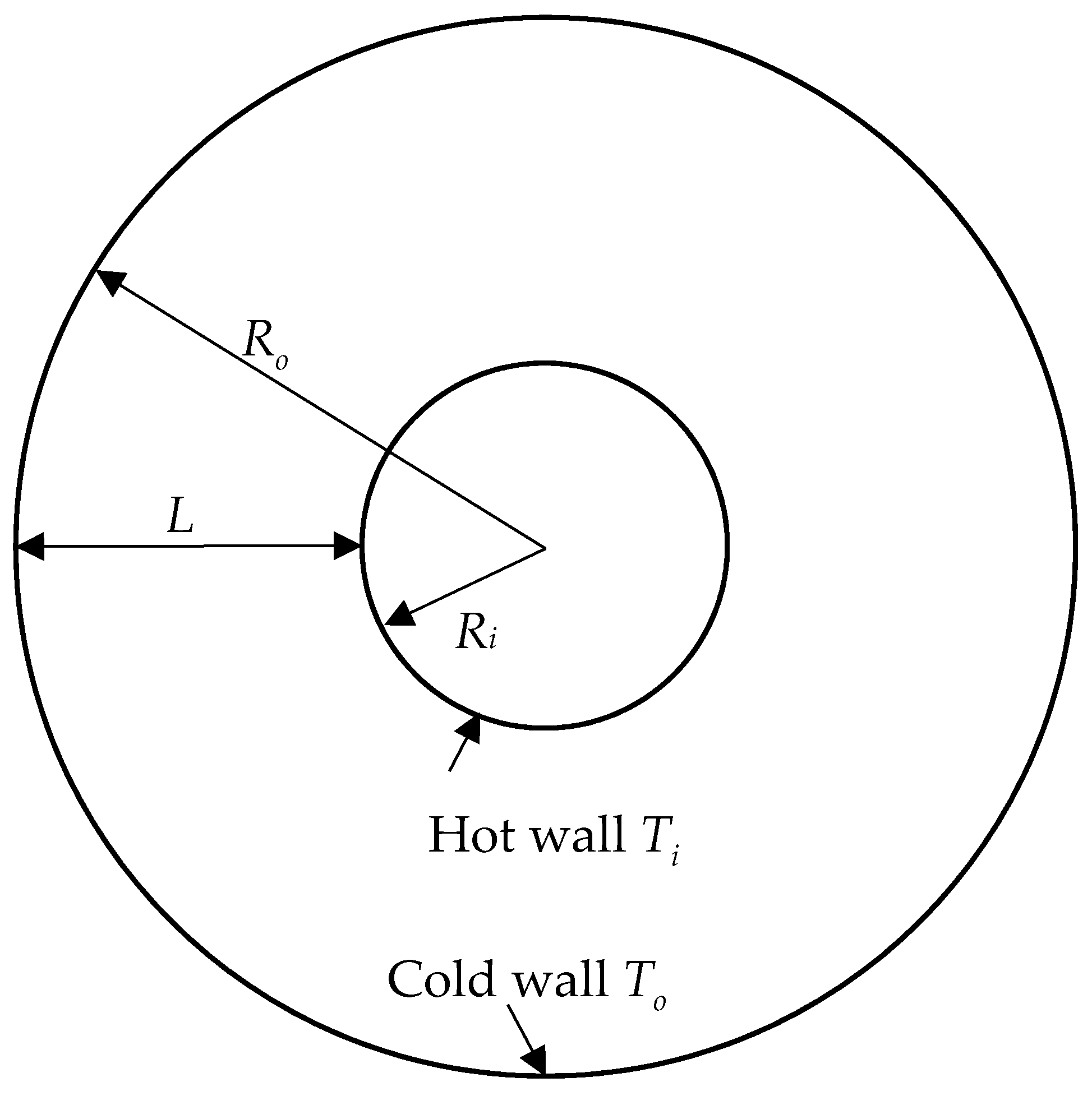
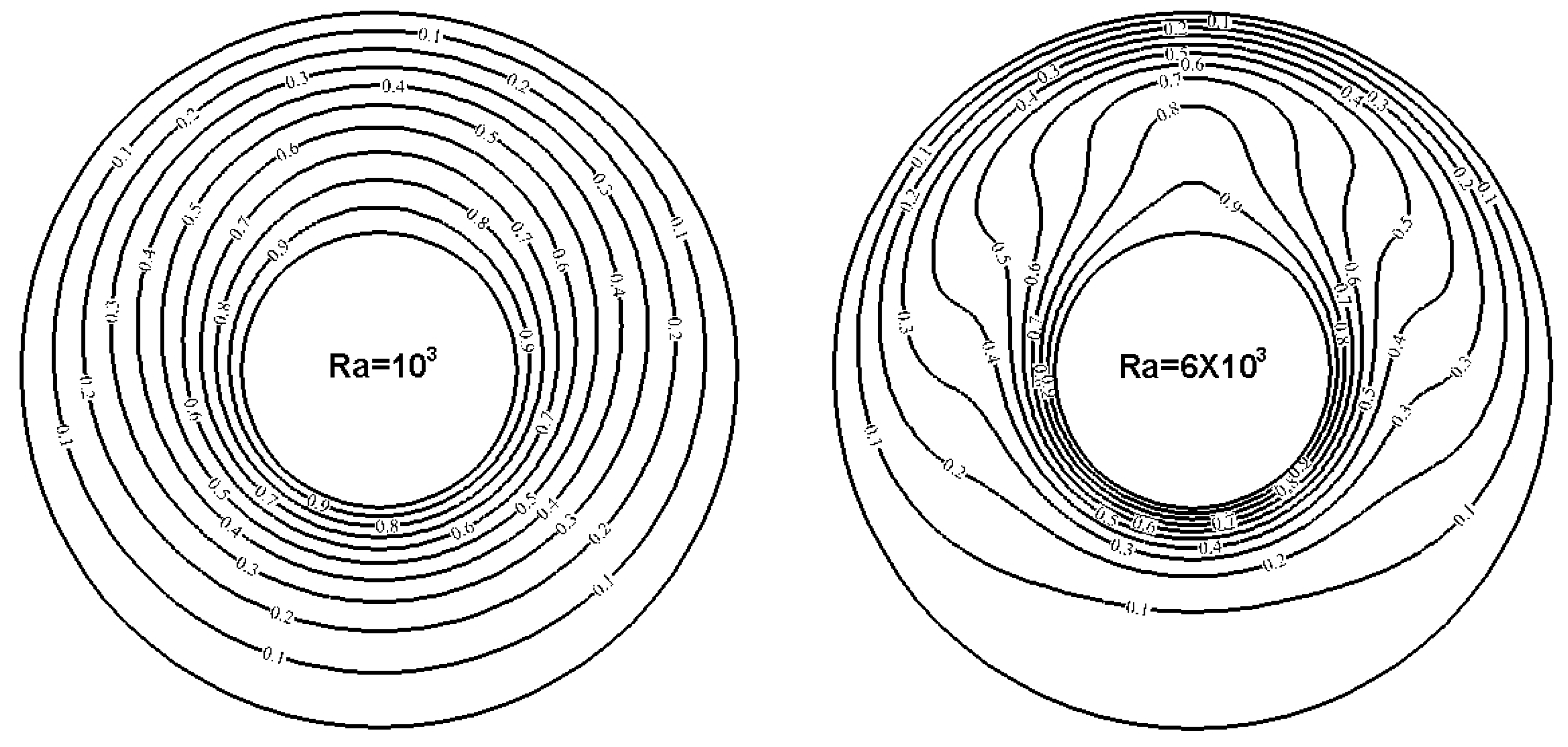
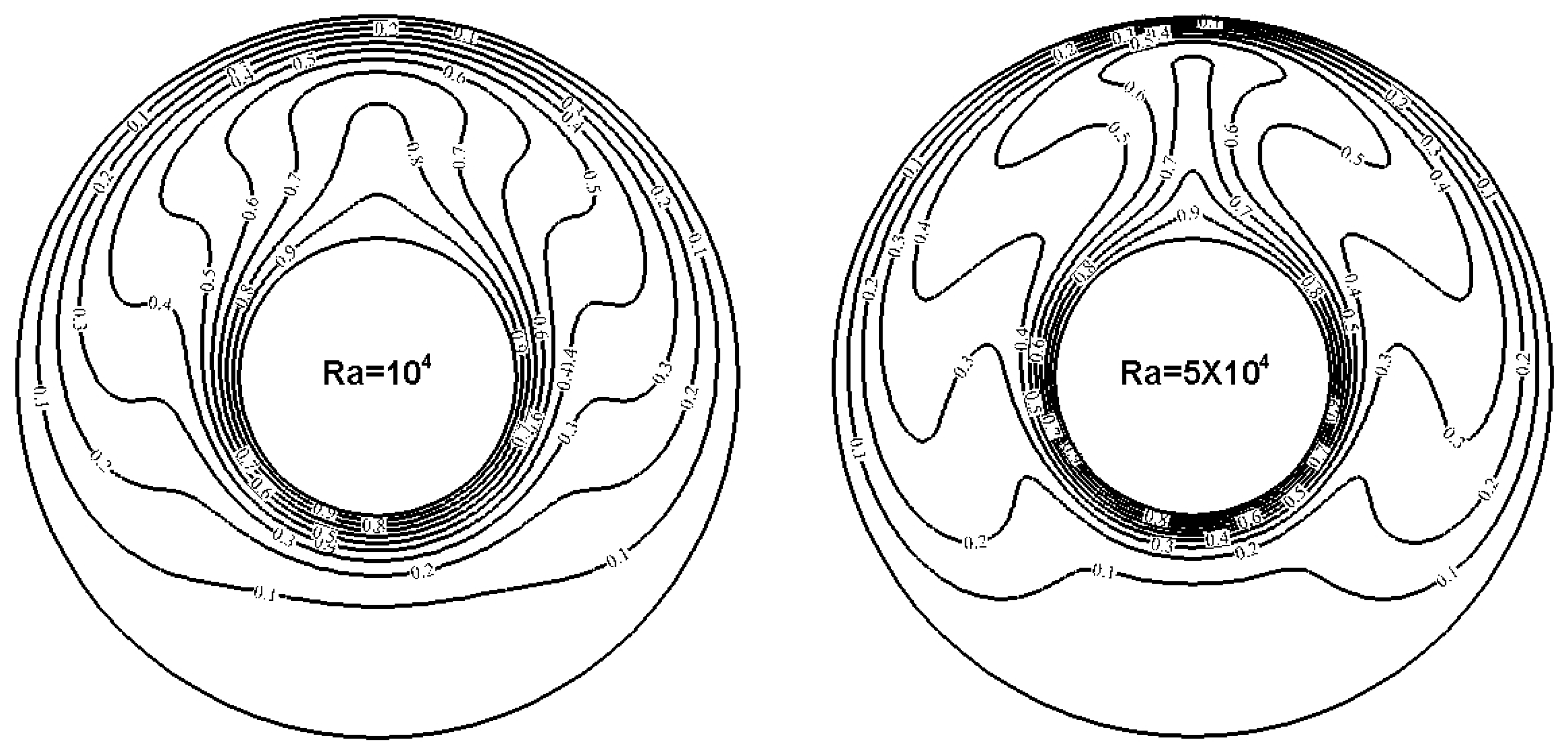
To test the flexibility of USTLBM on body-fitted mesh and on problems with curved boundaries, numerical test on natural convection in a concentric annulus is carried out in this section. Set-up of the problem is depicted in Figure 6. The gas filled between the concentric annulus is driven by the buoyance force that is induced by the temperature gradient between the hot inner circular cylinder and cold outer circular cylinder. Non-dimensional parameters in this problem include the aspect ratio Ar = R_o/R_i, the Prandtl number Pr = υ/χ and the Rayleigh number Ra = gβ(T_i−T_o)L³/υχ. In our simulations, we set Ar = 2.6 and Pr = 0.71; and four cases with different Rayleigh numbers of 10³, 6 × 10³, 10⁴ and 5 × 10⁴ are considered. To accurately describe the curved boundaries encountered in this problem, body fitted mesh with the mesh size of 251 × 81 is adopted in all simulations. Lagrangian interpolation algorithm is introduced in computational domain to evaluate functional values on locations where particles start the streaming process.

Isotherms at steady state of different cases are presented in Figure 7. It can be seen that our simulations keep the smoothness of the temperature field, which validates the stability of USTLBM. It is also observed that, with the increase of Rayleigh number, the isotherms are more squeezed to the lower part of the inner circular cylinder and the upper part of the outer circular cylinder. The reason is that, at higher Rayleigh number, the buoyance force induced by the temperature gradient has larger effect on the flow field, due to which the gas is pushed upward and compressed to the lower part of the inner cylinder and the upper part of the outer cylinder.

To quantify the correctness of USTLBM in this problem, the following equivalent heat conductivities are defined

$$\overline{k_{eqi}}=\frac{\ln \left(Ar\right)}{2\pi \left(Ar-1\right)}{\displaystyle {\int }_0^{2\pi }\frac{\partial T}{\partial r}\mathrm{d}\theta },\hspace{0.17em}\hspace{0.17em}\hspace{0.17em}\hspace{0.17em}\mathrm{for}\hspace{0.17em}\mathrm{the}\hspace{0.17em}\mathrm{inner}\hspace{0.17em}\mathrm{surface}$$

(75)

$$\overline{k_{eqo}}=\frac{Ar\cdot \ln \left(Ar\right)}{2\pi \left(Ar-1\right)}{\displaystyle {\int }_0^{2\pi }\frac{\partial T}{\partial r}\mathrm{d}\theta },\hspace{0.17em}\hspace{0.17em}\hspace{0.17em}\hspace{0.17em}\mathrm{for}\hspace{0.17em}\mathrm{the}\hspace{0.17em}\mathrm{outer}\hspace{0.17em}\mathrm{surface}$$

(76)

Calculated results in our simulations are tabulated in

Table 6. Comparison of average equivalent heat conductivity at different Rayleigh numbers.

Ra	Inner Cylinder, $\overline{{\mathit{k}}_{\mathit{e}\mathit{q}\mathit{i}}}$			Outer Cylinder, $\overline{{\mathit{k}}_{\mathit{e}\mathit{q}\mathit{o}}}$
	Kuehn and Goldstein [28]	Shu [29]	Present	Kuehn and Goldstein [28]	Shu [29]	Present
103	1.081	1.082	1.091	1.084	1.082	1.079
6 × 103	1.736	1.715	1.705	1.735	1.715	1.719
104	2.010	1.979	1.960	2.005	1.979	1.986
5 × 104	3.024	2.958	2.877	2.973	2.958	2.964

and compared with reference data in the literature [28,29]. It is noted that our computational results are in good agreement with the reference data. The relative errors are within 3%, which demonstrates the robustness of USTLBM in the present example on body-fitted mesh and with curved boundaries.

4.4. 3D Natural Convection in a Cubic Cavity

To further test the performance of USTLBM in three-dimensional problems, here we present the example of 3D natural convection in a cubic cavity. The physical set-up of the problem is a cubic cavity with its left and right walls, respectively, fixed on constant temperatures of T_h and T_c. On the other four walls, Neumann boundary condition with normal temperature gradient equal to zero is implemented. The non-dimensional parameters that determine the converged flow pattern are still the Rayleigh number and Prandtl number as defined in Equations (66) and (67). The average Nusselt number on the wall is defined as

$$N{u}_w=\frac{1}{L^2}{\displaystyle {\int }_0^L{\displaystyle {\int }_0^L\frac{\partial T}{\partial x}\mathrm{d}y\mathrm{d}z}}$$

(77)

Considering the numerical efficiency, non-uniform Cartesian mesh is adopted in this example. Two cases with high Rayleigh numbers of Ra = 10⁵ and 10⁶ are simulated.

Table 7. Comparisons of flow parameters for 3D natural convection in Ra = 10⁵.

Parameters	Grid	41 × 21 × 41	61 × 31 × 61	81 × 41 × 81	101 × 51 × 101	Reference [30,31,32,33,34]
Nuw	STLBM	4.349	4.367	4.361	4.355	4.337–4.464
	USTLBM	4.381	4.372	4.361	4.354
umax	STLBM	36.379	37.002	37.279	37.400	37.560–39.704
	USTLBM	36.213	36.960	37.264	37.396
wmax	STLBM	63.891	65.129	65.351	65.431	63.952–65.817
	USTLBM	64.487	65.262	65.380	65.446

and

Table 8. Comparisons of flow parameters for 3D natural convection in Ra = 10⁶.

Parameters	Grid	41 × 21 × 41	61 × 31 × 61	81 × 41 × 81	101 × 51 × 101	Reference [30,31,32,33,34]
Nuw	STLBM	7.622	8.255	8.509	8.605	8.640–8.770
	USTLBM	8.021	8.452	8.601	8.648
umax	STLBM	58.909	63.056	65.097	66.386	68.210–70.780
	USTLBM	57.143	62.432	64.962	66.327
wmax	STLBM	192.62	210.33	214.81	216.24	213.18–218.24
	USTLBM	204.05	214.67	216.45	217.10

give the average Nusselt number on the wall, the maximum horizontal velocity along the vertical centerline and the maximum vertical velocity along the horizontal centerline at different mesh sizes and Rayleigh numbers. It is observed that, be refining the mesh resolution, both USTLBM and STLBM can converge to the reference data [30,31,32,33,34]. Such performance indicates the robustness of USTLBM and STLBM on non-uniform mesh in three-dimensional scenarios. Careful comparisons reveal that, compared to our two-dimensional test of the natural convection in a square cavity (Section 4.1), the advantage of USTLBM over STLBM is not so obvious in this three-dimensional example. The possible reason is that, since the non-uniform mesh is adopted here, errors are inevitably introduced in the interpolation process, due to which the advantage of USTLBM in lowering numerical errors is counteracted and the results of USTLBM and STLBM are quite close. If uniform mesh is applied, the present USTLBM performs better than STLBM under the same mesh size, especially on coarser meshes (see

Table 9. Average Nusselt number on the wall for 3D natural convection in Ra = 10⁵.

Grid	SLBM	USLBM	References [30,31,32,33,34]
51 × 51 × 51	3.589	3.868	4.337–4.464
81 × 81 × 81	4.088	4.211
101 × 101 × 101	4.218	4.284

). Such evidence indicates that USTLBM can lower the numerical error of STLBM while maintaining the same order of accuracy in space.

5. Conclusions

In this paper, we present an unconditionally stable thermal lattice Boltzmann method (USTLBM) for numerical simulation of 2D/3D incompressible thermal flows. This method is developed from the recently proposed simplified thermal lattice Boltzmann method (STLBM) by truly ensuring the second-order of accuracy in time. Specifically, USTLBM is derived by reconstructing solutions to the macroscopic governing equations recovered from lattice Boltzmann equation and resolved in a predictor–corrector scheme. Final formulations of USTLBM only involve the equilibrium and the non-equilibrium distribution functions. In practical computation, the equilibrium distribution function is evaluated by the macroscopic variables, while the non-equilibrium term is approximated by the difference between two equilibrium distribution functions at different locations and time levels. Such treatment means that USTLBM can directly track the evolution of macroscopic variables rather than the distribution functions, which lowers the cost in virtual memories and facilitates implementation of physical boundary conditions.

Von Neumann stability analysis can be performed to prove that USTLBM is an unconditionally stable scheme. Numerical experiments are carried out on cases with coarse meshes and in high Rayleigh numbers to validate this conclusion. Accuracy test of USLTBM reveals that it ensures the second-order of accuracy in space while being able to achieve more accurate results than STLBM at the same mesh size.

Four numerical examples, including 2D natural convection in a square cavity, mixed convection in a lid-driven cavity, natural convection in a concentric annulus and 3D natural convection in a cubic cavity, are presented to validate the robustness and the flexibility of USTLBM. It turns out that the results obtained by USTLBM agree well with reference data in the literature; and the method can be flexibly coupled with Lagrangian interpolation algorithm to handle problems on non-uniform or body-fitted meshes and with curved boundaries.

References

1. Cengel, Y.A.; Ghajar, A.J.; Ma, H. Heat and Mass Transfer: Fundamentals and Applications, 4th ed.; McGraw-Hill: New York, NY, USA, 2011. [Google Scholar]
2. Anderson, J.D.; Wendt, J. Computational Fluid Dynamics; Springer: Berlin/Heidelberg, Germany, 1995. [Google Scholar]
3. Versteeg, H.K.; Malalasekera, W. An Introduction to Computational Fluid Dynamics: The Finite Volume Method; Pearson Education: England, UK, 2007. [Google Scholar]
4. Smith, G.D. Numerical Solution of Partial Differential Equations: Finite Difference Methods; Oxford University Press: Oxford, UK, 1985. [Google Scholar]
5. Alexander, F.J.; Chen, S.; Sterling, J. Lattice boltzmann thermohydrodynamics. Phys. Rev. E 1993, 47, R2249. [Google Scholar] [CrossRef]
6. Benzi, R.; Succi, S.; Vergassola, M. The lattice Boltzmann equation: Theory and applications. Phys. Rep. 1992, 222, 145–197. [Google Scholar] [CrossRef]
7. Chen, S.; Doolen, G.D. Lattice Boltzmann method for fluid flows. Annu. Rev. Fluid Mech. 1998, 30, 329–364. [Google Scholar] [CrossRef]
8. D’Humières, D. Multiple–relaxation–time lattice Boltzmann models in three dimensions. Philos. Trans. R. Soc. Lond. A Math. Phys. Eng. Sci. 2002, 360, 437–451. [Google Scholar] [CrossRef] [PubMed]
9. Aidun, C.K.; Clausen, J.R. Lattice-Boltzmann method for complex flows. Annu. Rev. Fluid Mech. 2010, 42, 439–472. [Google Scholar] [CrossRef]
10. He, X.; Luo, L.-S. Theory of the lattice Boltzmann method: From the Boltzmann equation to the lattice Boltzmann equation. Phys. Rev. E 1997, 56, 6811. [Google Scholar] [CrossRef]
11. Chen, Z.; Shu, C.; Wang, Y.; Yang, L.M.; Tan, D. A Simplified Lattice Boltzmann Method without Evolution of Distribution Function. Adv. Appl. Math. Mech. 2017, 9, 1–22. [Google Scholar] [CrossRef]
12. Chen, Z.; Shu, C.; Tan, D. A simplified thermal lattice Boltzmann method without evolution of distribution functions. Int. J. Heat Mass Transf. 2017, 105, 741–757. [Google Scholar] [CrossRef]
13. Peng, Y.; Shu, C.; Chew, Y. Simplified thermal lattice Boltzmann model for incompressible thermal flows. Phys. Rev. E 2003, 68, 026701. [Google Scholar] [CrossRef] [PubMed]
14. He, X.; Chen, S.; Zhang, R. A lattice Boltzmann scheme for incompressible multiphase flow and its application in simulation of Rayleigh–Taylor instability. J. Comput. Phys. 1999, 152, 642–663. [Google Scholar] [CrossRef]
15. Guo, Z.; Shu, C. Lattice Boltzmann Method and Its Applications in Engineering; World Scientific: Singapore, Singapore, 2013. [Google Scholar]
16. Succi, S. The Lattice Boltzmann Equation: For Fluid Dynamics and Beyond; Oxford University Press: Oxford, UK, 2001. [Google Scholar]
17. Guo, Z.; Zheng, C.; Shi, B. An extrapolation method for boundary conditions in lattice Boltzmann method. Phys. Fluids 2002, 14, 2007–2010. [Google Scholar] [CrossRef]
18. Sterling, J.D.; Chen, S. Stability analysis of lattice Boltzmann methods. J. Comput. Phys. 1996, 123, 196–206. [Google Scholar] [CrossRef]
19. D’Orazio, A.; Corcione, M.; Celata, G.P. Application to natural convection enclosed flows of a lattice Boltzmann BGK model coupled with a general purpose thermal boundary condition. Int. J. Thermal Sci. 2004, 43, 575–586. [Google Scholar] [CrossRef]
20. Wang, Y.; Shu, C.; Teo, C. Thermal lattice Boltzmann flux solver and its application for simulation of incompressible thermal flows. Comput. Fluids 2014, 94, 98–111. [Google Scholar] [CrossRef]
21. Shu, C.; Xue, H. Comparison of two approaches for implementing stream function boundary conditions in DQ simulation of natural convection in a square cavity. Int. J. Heat Fluid Flow 1998, 19, 59–68. [Google Scholar] [CrossRef]
22. De Vahl Davis, G. Natural convection of air in a square cavity: A bench mark numerical solution. Int. J. Numer. Methods Fluids 1983, 3, 249–264. [Google Scholar] [CrossRef]
23. Contrino, D.; Lallemand, P.; Asinari, P.; Luo, L.-S. Lattice-Boltzmann simulations of the thermally driven 2D square cavity at high Rayleigh numbers. J. Comput. Phys. 2014, 275, 257–272. [Google Scholar] [CrossRef]
24. Le Quéré, P. Accurate solutions to the square thermally driven cavity at high Rayleigh number. Comput. Fluids 1991, 20, 29–41. [Google Scholar] [CrossRef]
25. Wang, Y.; Yang, L.; Shu, C. From Lattice Boltzmann Method to Lattice Boltzmann Flux Solver. Entropy 2015, 17, 7713–7735. [Google Scholar] [CrossRef]
26. Cheng, T.; Liu, W.-H. Effect of temperature gradient orientation on the characteristics of mixed convection flow in a lid-driven square cavity. Comput. Fluids 2010, 39, 965–978. [Google Scholar] [CrossRef]
27. Bettaibi, S.; Kuznik, F.; Sediki, E. Hybrid lattice Boltzmann finite difference simulation of mixed convection flows in a lid-driven square cavity. Phys. Lett. A 2014, 378, 2429–2435. [Google Scholar] [CrossRef]
28. Kuehn, T.; Goldstein, R. An experimental and theoretical study of natural convection in the annulus between horizontal concentric cylinders. J. Fluid Mech. 1976, 74, 695–719. [Google Scholar] [CrossRef]
29. Shu, C. Application of differential quadrature method to simulate natural convection in a concentric annulus. Int. J. Numer. Methods Fluids 1999, 30, 977–993. [Google Scholar] [CrossRef]
30. Peng, Y.; Shu, C.; Chew, Y. A 3D incompressible thermal lattice Boltzmann model and its application to simulate natural convection in a cubic cavity. J Comput Phys. 2004, 193, 260–274. [Google Scholar] [CrossRef]
31. Fusegi, T.; Hyun, J.; Kuwahara, K.; Farouk, B. A numerical study of three-dimensional natural convection in a differentially heated cubical enclosure. Int. J. Heat Mass Transf. 1991, 34, 1543–1557. [Google Scholar] [CrossRef]
32. Wang, Y.; Shu, C.; Teo, C.J.; Wu, J.; Yang, L. Three-Dimensional Lattice Boltzmann Flux Solver and Its Applications to Incompressible Isothermal and Thermal Flows. Commun. Comput. Phys. 2015, 18, 593–620. [Google Scholar] [CrossRef]
33. Ha, M.Y.; Jung, M.J. A numerical study on three-dimensional conjugate heat transfer of natural convection and conduction in a differentially heated cubic enclosure with a heat-generating cubic conducting body. Int. J. Heat Mass Transf. 2000, 43, 4229–4248. [Google Scholar] [CrossRef]
34. Tric, E.; Labrosse, G.; Betrouni, M. A first incursion into the 3D structure of natural convection of air in a differentially heated cubic cavity, from accurate numerical solutions. Int. J. Heat Mass Transf. 2000, 43, 4043–4056. [Google Scholar] [CrossRef]
Figure 1. Illustration of D2Q9 and D3Q15 model.
Applsci 07 00277 g001
Figure 2. Physical configuration of 2D natural convection in a square cavity.
Applsci 07 00277 g002
Figure 3. Relative errors of volume averaged Nusselt numbers at different mesh spacing.
Applsci 07 00277 g003
Figure 4. Physical configuration of mixed convection in a lid-driven cavity.
Applsci 07 00277 g004
Figure 5. Isotherms and streamlines of mixed convection in a lid-driven cavity: (Left) isotherms; and (Right) streamlines.
Applsci 07 00277 g005aApplsci 07 00277 g005b
Figure 6. Illustration of the setup for natural convection in a concentric annulus.
Applsci 07 00277 g006
Figure 7. Isotherms for natural convection in a concentric annulus.
Applsci 07 00277 g007aApplsci 07 00277 g007b