Article

Gait Planning Research for an Electrically Driven Large-Load-Ratio Six-Legged Robot

1
College of Mechanical Engineering, Tianjin University of Technology and Education, Tianjin 300222, China
2
State Key Laboratory of Robotics and System, Harbin Institute of Technology, Harbin 150001, China
*
Authors to whom correspondence should be addressed.
Appl. Sci. 2017, 7(3), 296; https://doi.org/10.3390/app7030296
Submission received: 12 February 2017 / Revised: 11 March 2017 / Accepted: 16 March 2017 / Published: 18 March 2017

Abstract

:
Gait planning is an important basis for the walking of a legged robot. To improve the walking stability of multi-legged robots and to reduce the impact force between the foot and the ground, gait planning strategies are presented for an electrically driven large-load-ratio six-legged robot. First, the configuration and walking gait of the electrically driven large-load-ratio six-legged robot are designed. The higher-stable swing sequences of legs and typical walking modes are respectively obtained. Based on the Denavit-Hartenberg (D-H) method, the analyses of the forward and inverse kinematics are implemented. The mathematical models of the articulated rotation angles are respectively established. In view of the buffer device installed at the end of shin to decrease the impact force between the foot and the ground, an initial lift height of the leg is brought into gait planning when the support phase changes into the transfer phase. The mathematical models of foot trajectories are established. Finally, a prototype of the electrically driven large-load-ratio six-legged robot is developed. The experiments of the prototype are carried out regarding the aspects of the walking speed and surmounting obstacle. Then, the reasonableness of gait planning is verified based on the experimental results. The proposed strategies of gait planning lay the foundation for effectively reducing the foot–ground impact force and can provide a reference for other large-load-ratio multi-legged robots.

1. Introduction

In nature, the legged animal uses the coordinated motion of their legs to actualize from the current location to the goal location, which is called gait. Generally speaking, the types of gait will increase with the augmentation of legs. Then, the gait planning of legged robots will be more complex. Although the legged robot can have many types of gaits in theory, not every gait can make the robot stably and effectively walk. It is therefore necessary to carry out the analysis of the gait and motion planning. The different mobile system structures of legged robots often need different gait planning strategies. The gait planning of legged robots not only directly affects the consistency and stability, but also relates to the degree of energy dissipation.
Many researchers hope to obtain an excellent legged robot which can independently think and work like the animal. Presently, the walking of excellent multi-legged robots mainly depends on the sensing system, control strategy, initial gait planning, etc. The information from the legged robot and environment can be obtained by the sensing system. The initial gait planning is employed and repaired through the control strategy of the robot. Then, the walking of legged robots can be realized in structured and unstructured environments.
The large-load-ratio multi-legged robot can not only carry a variety of detection equipment to carry out the scientific exploration tasks, but can also play the role of the transporter. Hence, the terrain adaptability is needed for large-load-ratio multi-legged robots. To enhance the walking stability of the robot and reduce the impact force of the swing leg to the ground, the large-load-ratio multi-legged robot often requires the installation of an elastic cushion or rubber tire on the end of the foot. The spring and other elastic elements are often installed in the lower limb of the leg by comparing with the non-bearing small multi-legged robot. Hence, the buffer devices can be often found in many large-load-ratio multi-legged robots, such as Big Dog [1,2], COMET-IV [3,4], ATHLETE [5,6], and so on.
The gait planning of multi-legged robots is studied by many researchers. Erden [7] used the free gait generation algorithm to make a six-legged robot generate stable gaits based on the commanded velocity. The reinforcement learning was applied to the six-legged robot in real time. Leblebicioğlu [8] modified the conventional wave gaits. The modified versions of the wave gaits are more efficient than the conventional wave gaits. Ishikawa et al. [9] used a simplified neural network model called the associatron to deal with the gait motion planning problem on an irregular field for a six-legged robot. The viability of the proposed method was verified by the simulation and the experiments of the developed robot. Estremera et al. [10] presented the crab-type turning gaits for hexapod robots on uneven ground and forbidden zones. The turning gaits were tested by the SILO-6 walking robot. Satzinger et al. [11] proposed an end-to-end planning method that can achieve the teleoperated mobility of robot in complex environments. Fielding and Dunlop [12] extended the range of forward walking gaits of robots by adjusting the restrictedness controller. The range of wave gaits was then developed. The test experiment was carried out by a small hexapod “Hamlet”. Tedeschi and Carbone [13,14] addressed the design and operation of hexapod walking robots. The example of gait planning was provided through kinematic and dynamic features of Cassino hexapod leg operation. Sadati et al. [15] developed a motion planning algorithm for walking with passive knees. Although many researchers have performed a lot of research regarding the gait planning of the legged robots and have obtained effective planning strategies, the buffer device located at the shin is rarely considered in the gait planning. At present, we have not found reports in the literature that the initial lift height of the swing leg is introduced into the gait planning for large-load-ratio multi-legged robots.
Based on the above problems and the previous research on the legged robot [16,17,18,19], the initial lift height of the swing leg is brought forward and introduced into the research of the gait planning for an electrically driven large-load-ratio six-legged robot, which can lay the foundation for analyzing the foot force distribution and the power consumption of robot mobile systems under different gaits.
This article is divided into six sections. In Section 2, the configuration and walking gait are analyzed and designed for the electrically driven large-load-ratio six-legged robot. The higher-stability swing sequences of legs and the typical walking modes are respectively acquired. In Section 3, the analyses of the forward and inverse kinematics are executed based on the D-H method. The mathematical models are built for the articulated rational angles. In Section 4, the initial lift height of the swing leg is incorporated into the analysis of the gait planning. The mathematical models of the feet trajectories are established in the support phase and transfer phase, respectively. In Section 5, a prototype of the electrically driven large-load-ratio six-legged robot is developed. The gait planning strategies are written in C++ language and downloaded to the control system of the robot. The experiments of the walking speed and surmounting obstacle are actualized to verify the reasonableness of the gait planning strategies. In the final section, the conclusions are presented.

2. Configuration and Walking Gait of the Large-Load-Ratio Six-Legged Robot

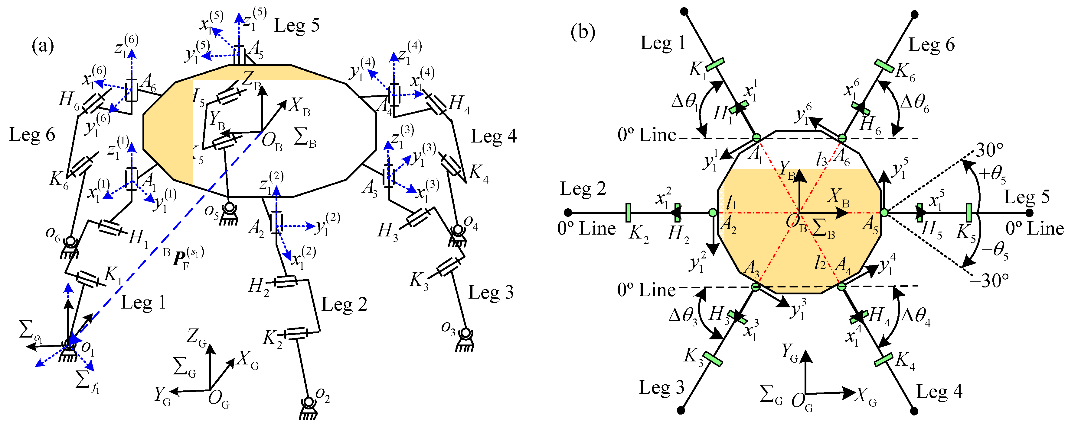
2.1. Configuration of the Large-Load-Ratio Six-Legged Robot

To conveniently carry out the analysis of the gait planning, the electrically driven large-load-ratio six-legged robot is called the large-load-ratio six-legged robot for short. The leg of the robot is designed based on the walking leg of a hexapod. Each leg has three joints, including an abductor joint, hip joint, and knee joint. The abductor joint, hip joint, and knee joint are respectively defined as Ai, Hi, and Ki (i = 1–6). Each leg is made up of three linkages: a coxa, thigh, and shin. The axis of the abductor joint runs parallel to the Z-axis. The axes of the hip joint and knee joint follow the direction of the Y-axis. To maintain the characteristics of universal walking, the configuration of the robot body is designed as a regular polygon. The mechanism of the robot and structure of the leg are respectively shown in Figure 1 and Figure 2.
In Figure 1, the body coordinate system of the robot is set as B located at the center of the body. The ground coordinate system is defined as G . The abductor joint coordinate system of leg i is regarded as A i , including the z 1 ( i ) -axis, x 1 ( i ) -axis, and y 1 ( i ) -axis. The z 1 ( i ) -axis is parallel to the ZB-axis of the body coordinate system. The x 1 ( i ) -axis is kept parallel with the coxa of leg i. The leg i lies in the plane z 1 ( i ) x 1 ( i ) . The foot coordinate system o i of leg i is parallel to the body coordinate system B . The foot coordinate system f i of leg i is parallel to the abductor joint coordinate system A i of leg i. The foot position matrix of leg sk is set as P F ( s k ) B in the body coordinate system. The coordinate system, which is located at the body and connects the body to the leg i, is regarded as 0 i . The coordinate system 0 i and the coordinate system A i are coincident with each other, when the rotating angle θi of the abductor joint of leg i is zero degrees.
In Figure 1, the 0° lines are kept parallel with the XB-axis of the B and pass through the origins of the coordinate systems of the abductor joints. The included angle ∆θi between the 0° line and leg i is defined as the initial angle of the abductor joint. The initial angle ∆θi can be used to set the initial position of the abductor joint when the robot begins to walk. The range of ∆θi is limited from 0° to 60°. θi is the rotation angle of the abductor joint based on the initial angle ∆θi. The initial angles ∆θ2 and ∆θ5 are always zero degrees for legs 2 and 5. The initial angles ∆θ1, ∆θ3, ∆θ4, and ∆θ6 can vary within their range, and they are equal to each other when the robot begins to walk. In Figure 2, the lengths of the coxa, thigh, and shin are set as lc, lt, and ls. The rotation angle of the abductor joint is set as θi. βi′ (i = 1–6) is regarded as the included angle between the coxa of leg i and the thigh of leg i. γi (i = 1–6) is regarded as the included angle between the thigh of leg i and the shin of leg i. The included angle between the coxa of leg i and the shin of leg i is defined as βi (i = 1–6). Then, the relations among βi′, γi, and βi can be obtained; they are βi = βi′ + γi and 0° ≤ βi′ ≤ βi ≤ 90°.
According to Figure 1, the angle between the coordinate system 0 i and the coordinate system B is defined as Φi for the leg i. Hence, the values of angle Φi are 120°, 180°, 240°, 300°, 360°, and 60° for legs 1, 2, 3, 4, 5, and 6, respectively. The rotation matrix and position matrix can then be obtained as,
R ( i ) 0 B = Rot ( z , Φ i ) = ( cos Φ i sin Φ i 0 sin Φ i cos Φ i 0 0 0 1 )
P 0 ( i ) B = ( P 0 x ( i ) B P 0 y ( i ) B P 0 z ( i ) B )
R ( i ) A B = ( R ( i ) 0 B R ( i ) A 0 ) 1 = ( Rot ( z , Φ i ) Rot ( z , θ i ) ) T = R ( i ) o f
where R ( i ) 0 B is the rotation matrix from the coordinate system 0 i to the body coordinate system B for the leg i, R ( i ) 0 B R 3 × 3 . P 0 ( i ) B is the position matrix form the coordinate system 0 i to the body coordinate system B for the leg i, P 0 ( i ) B R 3 × 1 . R ( i ) A B is the rotation matrix from the abductor joint coordinate system A i to the body coordinate system B for the leg i, R ( i ) A B R 3 × 3 . R ( i ) o f is the rotation matrix from the foot coordinate system o i to the foot coordinate system f i , R ( i ) o f R 3 × 3 . R ( i ) A 0 is the rotation matrix from the abductor joint coordinate system A i to the coordinate system 0 i , R ( i ) A 0 R 3 × 3 .

2.2. Typical Gait of the Large-Load-Ratio Six-Legged Robot

The gait of the six-legged robot is a static gait. The number of legs in the support phase should be no less than three at any time. To facilitate the gait analysis, su and tr are respectively regarded as the legs of the support phase and transfer phase. The relations are 3 ≤ u ≤ 6 and u + r = 6. The gait is called u foot gait when the number of legs is u in the support phase. The walking speed, step pitch, total number of legs, gait period, and duty ratio are respectively set as vR, s, n, T, and βR. Ts and Tt are defined as the time of the support phase and transfer phase. Generally speaking, the range of the duty ratio is from 0.5 to 1 for the six-legged robot. Then, the mathematical expression can be written about the walking speed of the robot.
v R = s T s = s β R T = s n T u
Based on Equation (4), it can be concluded that the three foot gait (or tripod gait) has a higher walking speed than the four foot gait (or quadrangular gait, tetrapod gait) and the five foot gait (or pentagon gait) when the walking speed and step pitch are constant. The parts of the gait parameters are listed in Table 1 for the large-load-ratio six-legged robot.
The tripod gait is the most common gait and the fastest gait for six-legged robots. The pentagon gait is the most stable gait and slowest gait for six-legged robots. Although the stability and walking speed of the quadrangular gait are between that of the tripod gait and the pentagon gait, the analysis complexity of the quadrangular gait is generally more than that of the other gaits. One period of the quadrangular gait includes three steps: 1/3 gait, 2/3 gait, and 3/3 gait (it can also be regarded as the last 1/3 gait). The stability and articulated torques need to be considered when the large-load-ratio six-legged robot passes a slope. The number of legs in the support phase should be two in the front and rear. Then, 18 kinds of higher-stable swing sequences of the legs, as shown in Table 2, can be obtained when the robot traverses a slope with the quadrangular gait.

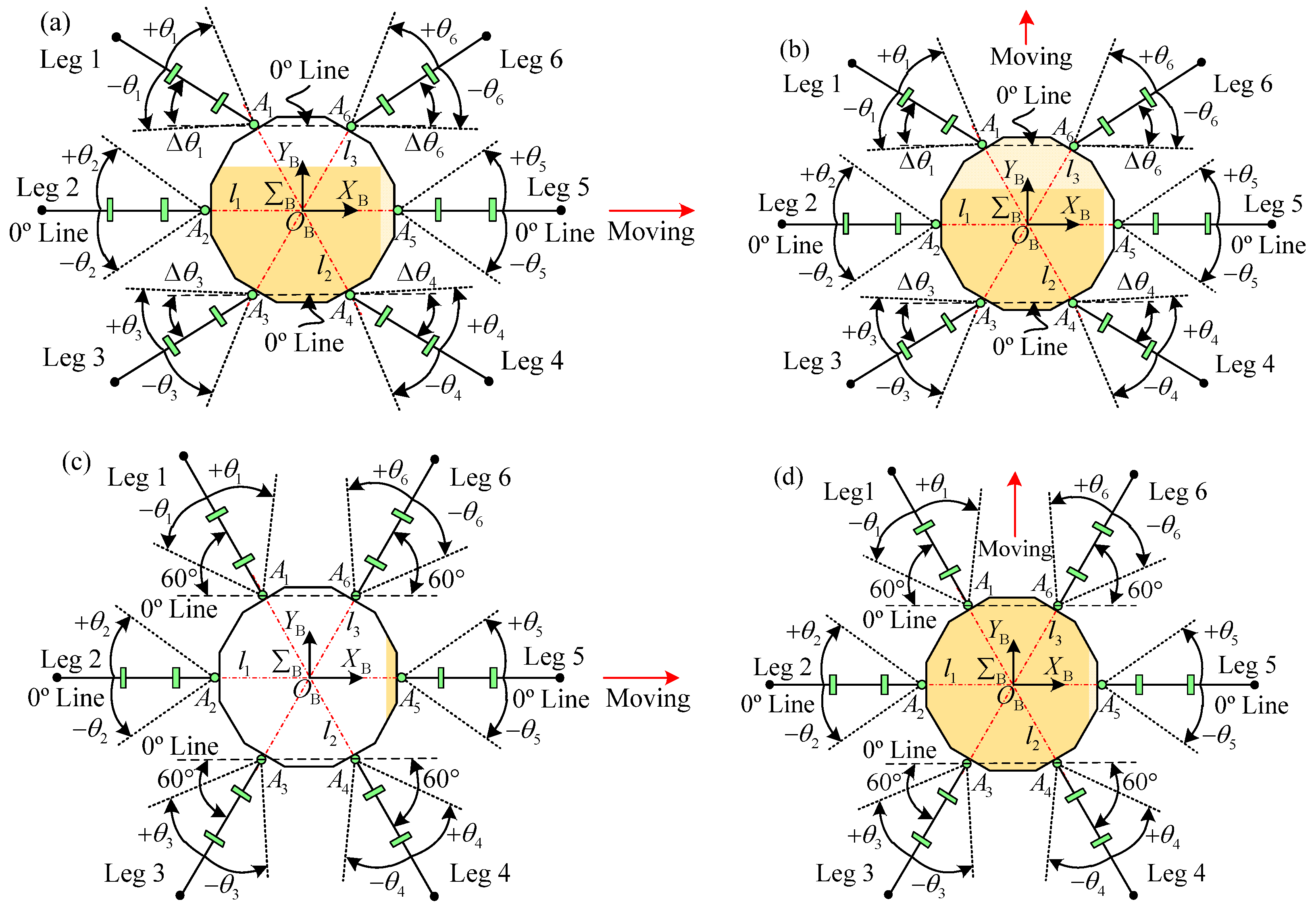
2.3. Walking Modes of the Large-Load-Ratio Six-Legged Robot

According to the configuration of the large-load-ratio six-legged robot, the walking modes can be divided into the crab type, ant type, crab–ant mixed type I, and crab–ant mixed type II; they are shown in Figure 3. The initial attitudes of the robot under the crab type and ant type can be arbitrarily set though the abductor joint initial angles of legs 1, 3, 4, and 6. The crab type and ant type can be respectively changed into the crab–ant mixed type I and crab–ant mixed type II, when the conditions are ∆θ1 = ∆θ3 = ∆θ4 = ∆θ6 = 60°. In Figure 3, +θi and −θi are defined as the front swing angle and rear swing angle on the basis of the ∆ θi. The straight lines l1, l2, and l3 are orthogonal to the relevant axes of the abductor joints.
Based on Figure 3, the contributions from the joints to the walking speed vR can be divided into non-contribution (NC), auxiliary contribution (AC), and main contribution (MC), as shown in Table 3, when the abductor joint initial angles ∆θi changes from 0° to 60°. To maintain the stability of the robot, the condition is set as ∆θ1 = ∆θ3 = ∆θ4 = ∆θ6. Then, the homogeneous joint on legs 1, 3, 4, and 6 has the same contribution to the walking speed of the robot.
According to Table 3, it can be concluded that the walking speed of the robot is directly provided by the hip joints and knee joints of legs 2 and 5 under the crab type and crab–ant mixed type I. The abductor joints of legs 2 and 5 do not contribute to the walking of the robot. When the articulated actuating devices output the large torques under constant power, the walking speed of the robot is limited by the hip joints and knee joints of legs 2 and 5. Then, we can see that the crab type and crab–ant mixed type I are not conducive for high-speed walking of the robot, but they are suited for climbing slopes and other tasks. Based on the ant-type walking mode, the walking speed of the robot is mainly provided by the abductor joints. The hip joints and knee joints only play an auxiliary role. It can be concluded that the maximum walking speed of the robot is best realized under the ant type. The crab–ant mixed type I and crab–ant mixed type II are more stable than the crab type and ant type through analyzing the stability margin of the robot.

3. Kinematics Analysis of the Large-Load-Ratio Six-Legged Robot

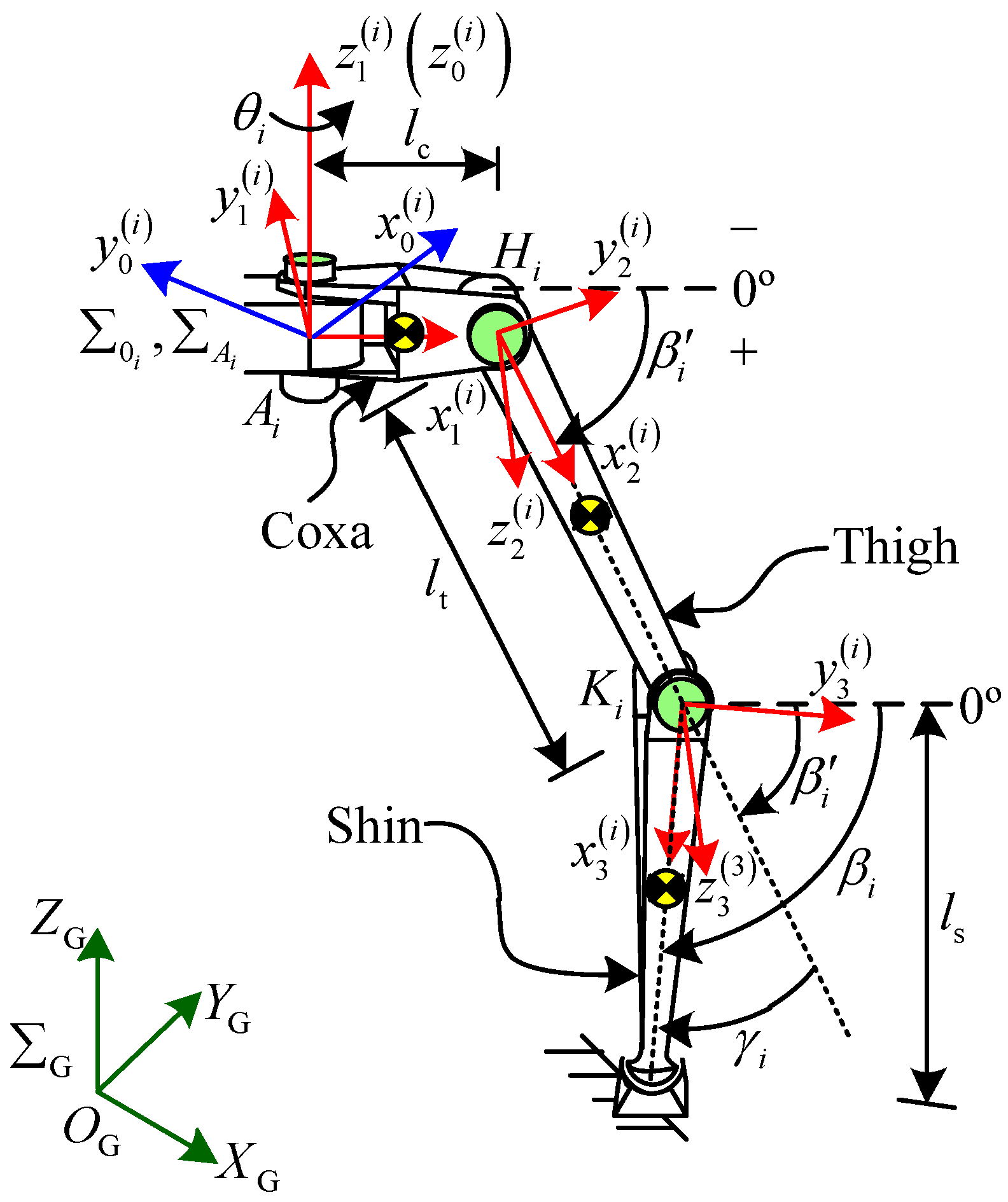
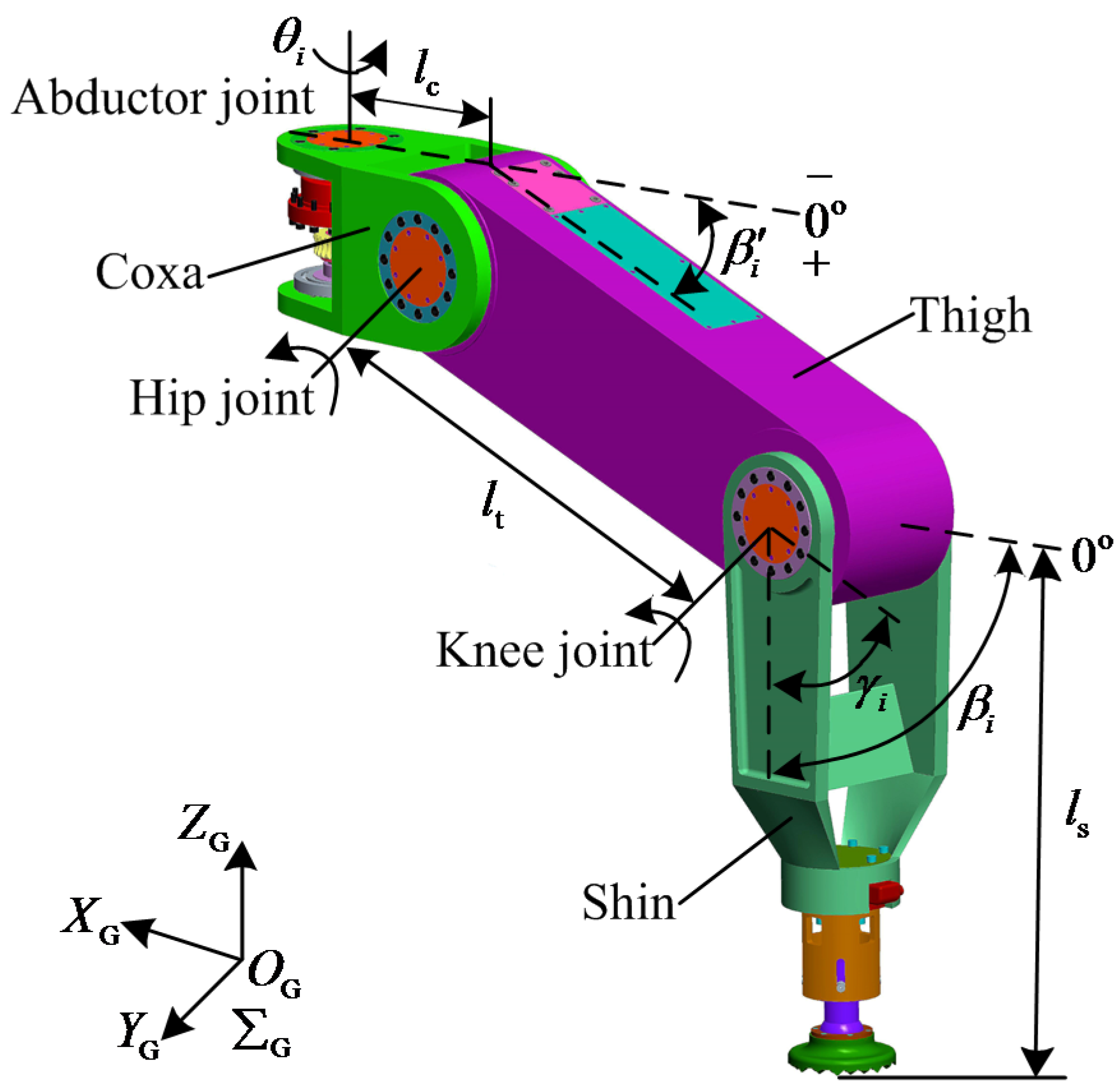
3.1. D-H Model of the Robot Single Leg

The D-H model of the leg i is shown in Figure 4. To elaborate on the kinematics analysis of the robot, the coordinate systems of the abductor joint Ai, hip joint Hi, and knee joint Ki are further defined as A i ( A i x 1 ( i ) y 1 ( i ) z 1 ( i ) ) , H i ( H i x 2 ( i ) y 2 ( i ) z 2 ( i ) ) , and K i ( K i x 3 ( i ) y 3 ( i ) z 3 ( i ) ) , respectively. The coordinate system 0 i can also be expressed as 0 i ( 0 i x 0 ( i ) y 0 ( i ) z 0 ( i ) ) . In Figure 4, H expresses the distance from the body centroid OB to the ground. It can be seen that the relation is hi = H. The axes of the abductor joints are kept parallel with the ZG-axis when the body bottom is parallel to the ground. The y 1 ( i ) -axis is kept parallel with the axes of the hip joint and knee joint of leg i.
To avoid the interferences caused by the rotation of the joints, the ranges of θi, βi, and βi are set as −30° to 30°, −90° to 90°, and from 0° to 150° based on the interval of the initial angle ∆θi, respectively. The coordinate system 0 i is coincident with the coordinate system A i when the value of the abductor joint is zero degrees for the leg i. The positive and negative values of the joint angle depend on the specified joint steering. The parameters of the D-H model of leg i are shown in Table 4.

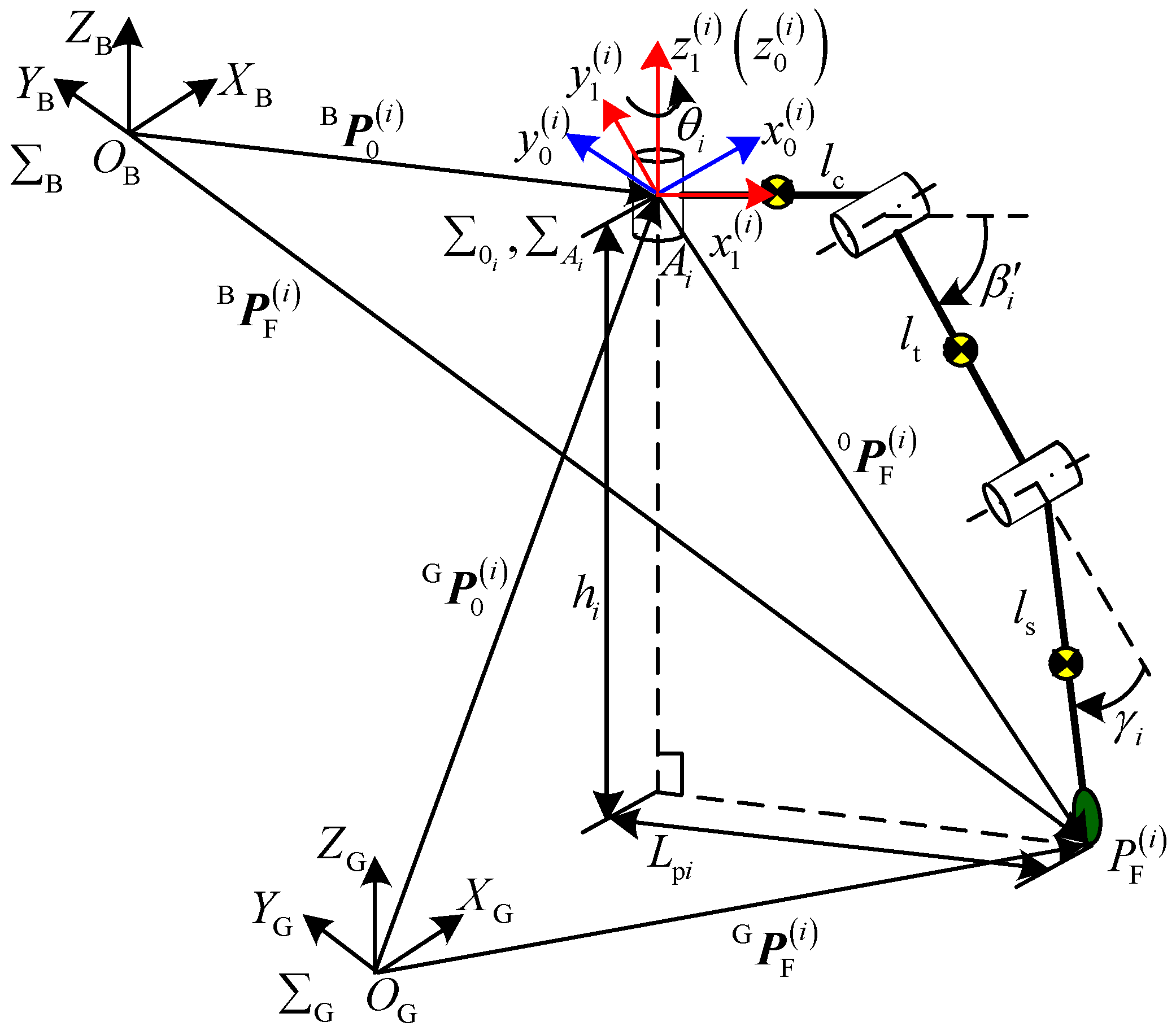
3.2. Forward Kinematics Analysis of the Large-Load-Ratio Six-Legged Robot

The foot position of leg i can be solved when the body posture and joint angles of each leg have been obtained. The analysis of the forward kinematics can be performed for the large-load-ratio six-legged robot. The transformation matrix of leg i between the joint j − 1 and the joint j is written as follows,
T ( i ) j j 1 = ( c θ j ( i ) s θ j ( i ) 0 a j 1 ( i ) s θ j ( i ) c α j 1 ( i ) c θ j ( i ) c α j 1 ( i ) s α j 1 ( i ) d j ( i ) s α j 1 ( i ) s θ j ( i ) s α j 1 ( i ) c θ j ( i ) s α j 1 ( i ) c α j 1 ( i ) d j ( i ) c α j 1 ( i ) 0 0 0 1 )
where c θ j ( i ) , s θ j ( i ) , c α j 1 ( i ) , and s α j 1 ( i ) are the abbreviations for cos θ j ( i ) , sin θ j ( i ) , cos α j 1 ( i ) , and sin α j 1 ( i ) , respectively .
The transformation matrices among the joints of leg i can be obtained when the parameters of the D-H model are substituted into Equation (5). Then,
T ( i ) 1 0 = ( cos θ i sin θ i 0 0 sin θ i cos θ i 0 0 0 0 1 0 0 0 0 1 )
T ( i ) 2 1 = ( cos β i sin β i 0 l c 0 0 1 0 sin β i cos β i 0 0 0 0 0 1 )
T ( i ) 3 2 = ( cos γ i sin γ i 0 l t sin γ i cos γ i 0 0 0 0 1 0 0 0 0 1 )
Based on Equations (6)–(8), the transformation matrix T ( i ) 3 0 from the coordinate system K i to the coordinate system 0 i can then be gained for the leg i,
T ( i ) 3 0 = ( c θ i c β i c θ i s β i s θ i l t c θ i c β i + l c c θ i s θ i c β i s θ i s β i c θ i l t s θ i c β i + l c s θ i s β i c β i 0 l t s β i 0 0 0 1 )
where c θ i , s θ i , c β i , s β i , c β i , and s β i are the abbreviations for cos θ i , sin θ i , cos β i , sin β i , cos β i , and sin β i , respectively.
The coordinate matrix P F ( i ) 3 of the foot of leg i can be written in the coordinate system K i of the knee joint. Then,
P F ( i ) 3 = ( l s 0 0 1 ) T
The transformation matrix T ( i ) 0 B from the coordinate system 0 i to the coordinate system B of the body can then be obtained as follows,
T ( i ) 0 B = ( R ( i ) 0 B P 0 ( i ) B O 1 ) R 4 × 4
where R ( i ) 0 B is the rotation matrix from the coordinate system 0 i to the coordinate system B of the body, R ( i ) 0 B R 3 × 3 . P 0 ( i ) B is the position matrix from the coordinate system 0 i to the coordinate system B of the body, P 0 ( i ) B R 3 × 1 . O is the zero matrix.
The foot position matrix P F ( i ) B of leg i can then be written under the coordinate system B of the body,
P F ( i ) B = T ( i ) 0 B T ( i ) 3 0 P F ( i ) 3 = ( cos ( Φ i + θ i ) ( l s cos β i + l t cos β i + l c ) + P 0 x ( i ) B sin ( Φ i + θ i ) ( l s cos β i + l t cos β i + l c ) + P 0 y ( i ) B l s sin β i + l t sin β i + P 0 z ( i ) B 1 )
Based on Equation (12), the forward kinematics of robot can be solved. When the articulated rotation angles have been obtained for the abductor joint, hip joint, and knee joint of leg i, the mathematical expression can be written for the position components of the foot in the directions of x, y, and z. Then,
P F x ( i ) B = cos ( Φ i + θ i ) ( l s cos β i + l t cos β i + l c ) + P 0 x ( i ) B
P F y ( i ) B = sin ( Φ i + θ i ) ( l s cos β i + l t cos β i + l c ) + P 0 y ( i ) B
P F z ( i ) B = l s sin β i + l t sin β i + P 0 z ( i ) B
According to the coordinate system G for the ground, the position matrix P F ( i ) G of the foot of leg i can then be expressed as follows,
P F ( i ) G = T ( i ) B G P F ( i ) B = ( R ( i ) B G P B ( i ) G O 1 ) ( P F x ( i ) B P F y ( i ) B P F z ( i ) B 1 )
where T ( i ) B G is the transformation matrix from the coordinate system B of the body to the coordinate system G of the ground, T ( i ) B G R 4 × 4 . R ( i ) B G is the rotation matrix from the coordinate system B of the body to the coordinate system G of the ground, R ( i ) B G R 3 × 3 . P B ( i ) G is the translation matrix from the coordinate system B of the body to the coordinate system G of the ground, P B ( i ) G R 3 × 3 .

3.3. Inverse Kinematics Analysis of the Large-Load-Ratio Six-Legged Robot

The walking of the large-load-ratio six-legged robot can be realized by controlling the driving joints of each leg in the support phase and transfer phase, which involves the inverse kinematics of the robot. When the robot walks using the static gait, the number of legs in the support phase needs to satisfy the constraint: 3 ≤ u ≤ 6. Then, a six degrees of freedom (6–DOF) parallel platform u–RRRS is composed by the ground, body of the robot, and u legs. The rotation angles of the joints can be solved under the feet trajectories of the support phase and transfer phase. The posture of leg i is shown in Figure 5 for the large-load-ratio six-legged robot.
In Figure 5, hi represents the distance from the coordinate origin of A i to the ground. Lpi is defined as the span which is the projection length of the leg i in the coordinate system A i of the abductor joint. Based on Figure 5, the position matrix P F ( i ) G from the foot of leg i to the coordinate system G of the ground can be obtained. Then,
P F ( i ) G = P 0 ( i ) G + P F ( i ) 0 = T ( i ) B G P 0 ( i ) B + P F ( i ) 0
where P 0 ( i ) G is the position matrix from the coordinate system 0 i to the coordinate system G of the ground, and P 0 ( i ) G = T ( i ) B G P 0 ( i ) B . P F ( i ) 0 is the position matrix of the foot of leg i in the coordinate system 0 i .
Based on Equation (17), the position matrix P F ( i ) 0 can be written as follows,
P F ( i ) 0 = P F ( i ) G T ( i ) B G P 0 ( i ) B
When the foot trajectory of leg i has been determined in the gait period, the position matrix P F ( i ) G of the foot can be obtained. Hence, the rotation angles of the abductor joint, hip joint, and knee joint are solved for the leg i. Then,
{ θ i = arctan ( P F y ( i ) B P 0 y ( i ) B P F x ( i ) B P 0 x ( i ) B ) Φ i γ i = arccos ( ξ l t 2 2 l s l t ) β i = arcsin ( 2 l t ( P F z ( i ) B P 0 z ( i ) B ) ( ξ + l t 2 ) 2 + 4 l s 2 l t 2 ( ξ l t 2 ) ) arctan ( 4 l s 2 l t 2 ( ξ l t 2 ) ξ + l t 2 ) ξ = ( ( P F x ( i ) B P 0 x ( i ) B ) 2 + ( P F y ( i ) B P 0 y ( i ) B ) 2 l c ) 2 + ( P F z ( i ) B P 0 z ( i ) B ) 2 l s 2

4. Gait Planning of the Large-Load-Ratio Six-Legged Robot

The large-load-ratio six-legged robot walks through the periodic swing and support of its legs. Each leg has a state between the support phase and the transfer phase at any time. Hence, the time sequence problem of the legs can be solved by gait planning. The legs of the robot have the same structure. Then, the planning method of the legs in the same phase is the same as in a gait period. To facilitate the gait planning, the initial position of the foot is defined as the reference position. Due to several motion models for the large-load-ratio six-legged robot, the reference position of the foot can be changed at any time.
The anterior extreme position (AEP) and posterior extreme position (PEP) are brought into the gait planning. s is defined as the step pitch from the AEP to the PEP. The organization principles of the gait planning are set up for the support phase and transfer phase. Firstly, the foot that has the shortest distance from the PEP is the first to enter the transfer phase. Secondly, the support phase and the transfer phase are periodic alternations. Actually, the AEP and PEP can be exchanged with each other, and they depend on the reference position of the foot and motion vector a. The AEP is the reference position of the foot plus the motion vector a. The PEP is the reference position of the foot minus the motion vector a. The length of the motion vector a is half of the step pitch s.
To reduce the impact force between the foot and the ground, a buffer device is installed on the end of each shin. The initial lift height of the leg is introduced to eliminate the influence of the buffer mechanism when the support phase changes into the transfer phase. The mopping phenomenon of the foot can be prevented. The initial lift height of the leg is favorable for striding over the larger obstacles and improving the terrain trafficability of the robot. The maximum swing height and initial lift height of the leg are respectively defined as hT-max and hTB. The relation between the hT-max and the hTB is 0 ≤ hTBhT-max. The coordinates of the foot, reference position, and motion vector a are respectively set as ( P F x 1 ( i ) B , P F y 1 ( i ) B , P F z 1 ( i ) B ) , ( P F x 0 ( i ) B , P F y 0 ( i ) B , P F z 0 ( i ) B ) , and (Bax, Bay, Baz) in the coordinate system B of the body.

4.1. Motion Planning of the Tripod Gait

The number of legs is three in the support phase. The duty ratio βR is 1/2. Legs 2, 4, and 6 are located in the support phase when legs 1, 3, and 5 are in the transfer phase, and vice versa. The feet trajectories of leg i between the AEP and the PEP are shown in Figure 6 for the support phase and transfer phase.
Based on Figure 6, the foot of leg i in the transfer phase swings from the current position to the AEP. Then, the foot of leg i in the support phase supports from the current position to the PEP along the opposite direction of the motion vector a. To ensure that the support foot does not cross the PEP in the first gait period of the robot, the first support distance in the support phase can be calculated from the current position to the PEP. To maintain the same support distance in the later gait period, the next support distance in the support phase is obtained based on the motion vector a.

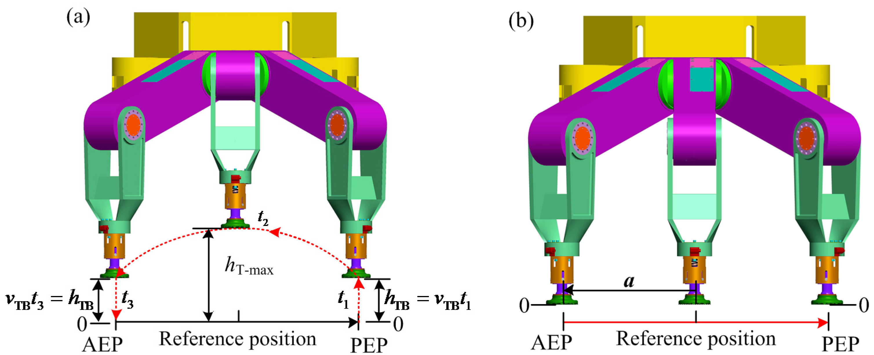
4.1.1. Motion Planning of the Transfer Phase

The foot of the transfer phase swings along a curve from the PEP to the AEP. Due to the arbitrary initial state for the swing leg, the moving trajectory of leg i in the transfer phase is the curve from the arbitrary position to the AEP. Two constraint conditions need to be considered in the motion planning of the transfer phase. Firstly, the velocity value of the foot is zero at the AEP and the PEP. Secondly, the acceleration curve of the foot has no the jump in the swing process of the leg. Generally, the energy consumption of the support phase is much larger than that of the transfer phase when the walking speed of robot is not high. Based on the research results of Nishii [20] and Lin [21], we find that there is little difference between the foot trajectory of the swing leg and the cosine curve. Hence, cosine programming is employed for the gait planning in this article.
Owing to the initial lift height hTB, the foot trajectory of the leg i can be divided into three parts in the transfer phase. In the first part, the foot of the leg i chooses the velocity vBT to uplift from 0 to hTB along the ZB direction during the time 0−t1. In the second part, the foot of the leg i moves to the AEP along the cosine curve during the time t1t2. In the third part, the foot of the leg i selects the velocity vBT to fall from hTB to 0 along the ZB direction during the time t2T/2. Then, the leg i is completely turned into the support leg.
In the first part, the mathematical model of the foot trajectory can be written for the leg i in a period of the tripod gait as follows,
{ X T 1 B = P F x 1 ( i ) B Y T 1 B = P F y 1 ( i ) B Z T 1 B = v TB t + P F z 1 ( i ) B 0 t t 1
In the second part, the mathematical model of the foot trajectory can be written for the leg i in a period of the tripod gait as follows,
{ X T 2 B = ( P F x 0 ( i ) B + a x B P F x 1 ( i ) B ) 2 × ( cos ( π t 2 t 1 ( t + t 2 2 t 1 ) ) + 1 ) + X T 1 B Y T 2 B = ( P F y 0 ( i ) B + a y B P F y 1 ( i ) B ) 2 × ( cos ( π t 2 t 1 ( t + t 2 2 t 1 ) ) + 1 ) + Y T 1 B Z T 2 B = ( h T - max h TB ) 2 × ( cos ( 2 π t 2 t 1 ( t + t 2 2 t 1 ) ) 1 ) + Z T 1 B t 1 t t 2
In the third part, the mathematical model of the foot trajectory can be written for the leg i in a period of the tripod gait as follows,
{ X T 3 B = X T 2 B Y T 3 B = Y T 2 B Z T 3 B = Z T 2 B v TB t t 2 t T / 2

4.1.2. Motion Planning of the Support Phase

The foot of the support phase supports from the AEP to the PEP. The motion direction of the support phase is opposite to that of the transfer phase. To make the robot in any state quickly enter the support phase, the support distance of the foot is set as 2a along the opposite direction of the motion vector a. Cosine programming is also selected for the support phase. The mathematical model of the foot trajectory in the support phase can then be written for the leg i under the tripod gait as follows,
{ X S B = a x B ( cos ( 2 π T t ) + 1 ) + P F x 1 ( i ) B Y S B = a y B ( cos ( 2 π T t ) + 1 ) + P F y 1 ( i ) B Z S B = P F z 1 ( i ) B T / 2 t T

4.2. Motion Planning of the Quadrangular Gait

Based on Table 2, the motion planning of the quadrangular gait is implemented for the large-load-ratio six-legged robot. Cosine programming is employed for the foot trajectory of the robot. The leg which has the minimum distance from the PEP is stipulated to first enter the transfer phase. The duty ratio βR is 2/3. Each leg needs to fulfill a swing task and two support tasks in a period of the quadrangular gait.
The foot trajectory of the leg i can be divided into three parts in the transfer phase. In the first part, the foot of the leg i chooses the velocity vBT to uplift from 0 to hTB along the ZB direction during the time 0−t1. In the second part, the foot of the leg i moves to the AEP along the cosine curve during the time t1t2. In the third part, the foot of the leg i selects the velocity vBT to fall from hTB to 0 along the ZB direction during the time t2T/3. Then, the leg i is completely turned into the support leg. The motion planning of the leg i under the quadruped gait is the same as that of the tripod gait in the transfer phase. Although the mathematical models of the foot trajectories under the tripod gait can be directly applied to the quadruped gait, the total swing time T/2 of leg i under the tripod gait needs to be changed to T/3 under the quadrangular gait.
When the motion vector a is constant, the support distance of leg i is changed from 2a under the tripod gait to a under the quadrangular gait. The total support distance of the support phase is 2a along the opposite direction of the motion vector a. The mathematical model of the foot trajectory in the support phase can then be written for the leg i under the quadrangular gait as follows,
{ X S B = a x B ( cos ( 3 π 2 T t π 2 ) 1 ) + P F x 1 ( i ) B Y S B = a y B ( cos ( 3 π 2 T t π 2 ) 1 ) + P F y 1 ( i ) B Z S B = P F z 1 ( i ) B T / 3 t T

4.3. Motion Planning of the Pentagon Gait

Each leg needs to finish a swing task and five support tasks in a period of the pentagon gait. The duty ratio βR is 5/6. Then, each leg can be regarded as a group. The leg which has the minimum distance from the PEP is stipulated to first enter the transfer phase. The cosine programming is employed for the motion planning of the pentagon gait.
The foot trajectory of the leg i can be divided into three parts in the transfer phase. In the first part, the foot of the leg i selects the velocity vBT to uplift from 0 to hTB along the ZB direction during the time 0−t1. In the second part, the foot of the leg i moves to the AEP along the cosine curve during the time t1t2. In the third part, the foot of the leg i uses the velocity vBT to fall from hTB to 0 along the ZB direction during the time t2T/6. Then, the leg i is completely turned into the support leg. The motion planning of the leg i under the pentagon gait is the same as that of the tripod gait in the transfer phase. Although the mathematical models of the foot trajectories under the tripod gait can be directly applied to the pentagon gait, the total swing time T/2 of leg i under the tripod gait needs to be changed to T/6 under the pentagon gait.
When the motion vector a is constant, the support distance of the leg i is changed from 2a under the tripod gait to 2a/5 under the pentagon gait. The total support distance of the support phase is 2a along the opposite direction of the motion vector a. The mathematical model of the foot trajectory in the support phase can then be written for the leg i under the pentagon gait as follows,
{ X S B = a x B ( cos ( 6 π 5 T t + 4 π 5 ) + 1 ) + P F x 1 ( i ) B Y S B = a y B ( cos ( 6 π 5 T t + 4 π 5 ) + 1 ) + P F y 1 ( i ) B Z S B = P F z 1 ( i ) B T / 6 t T

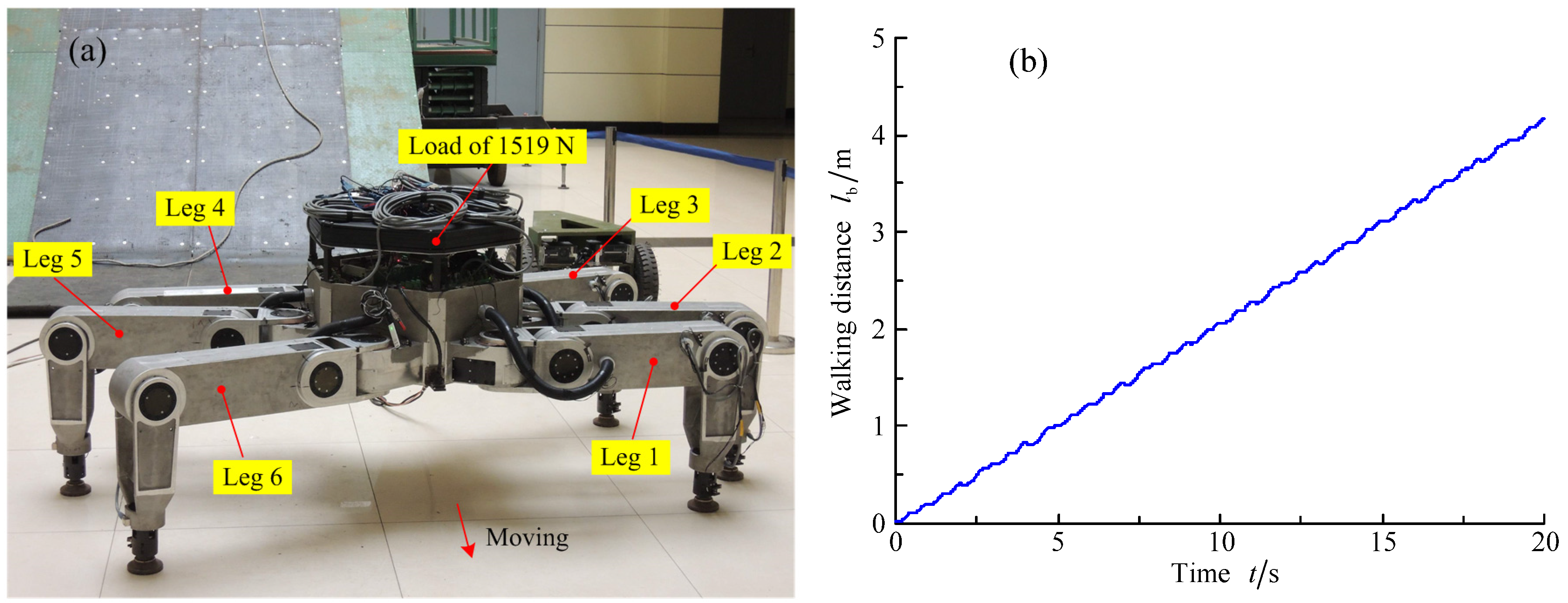
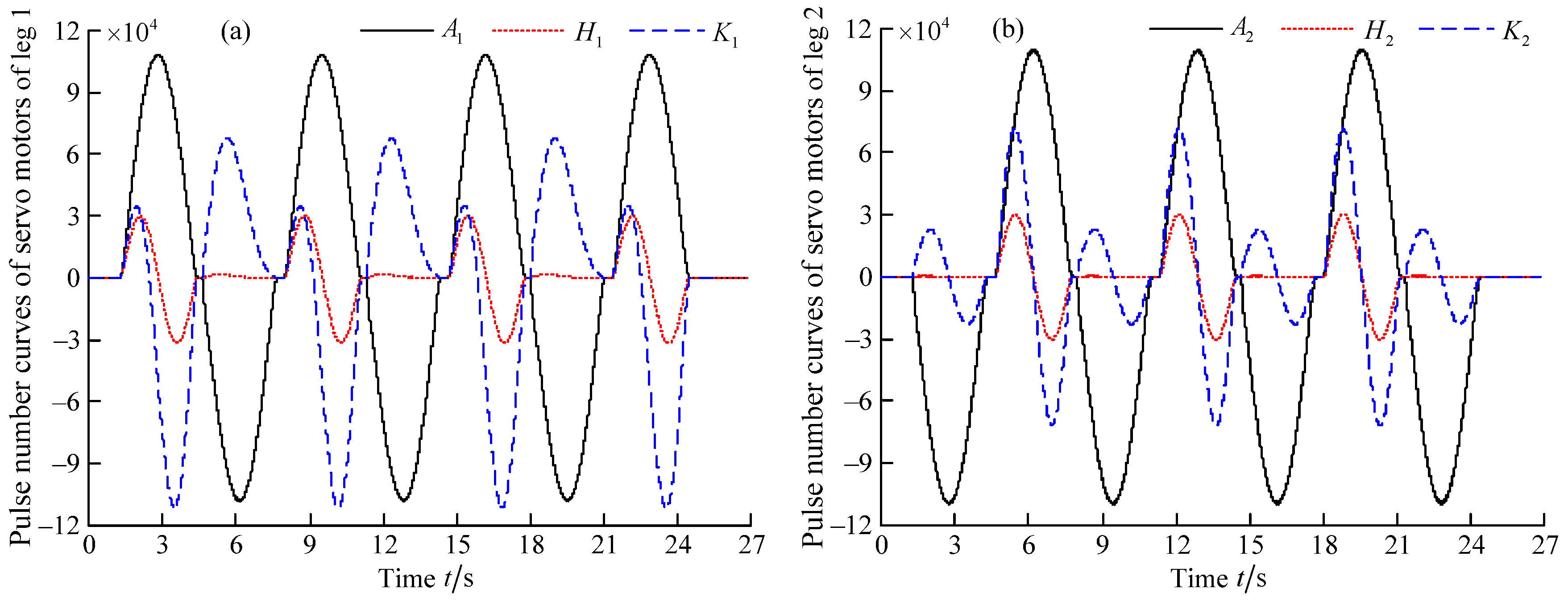
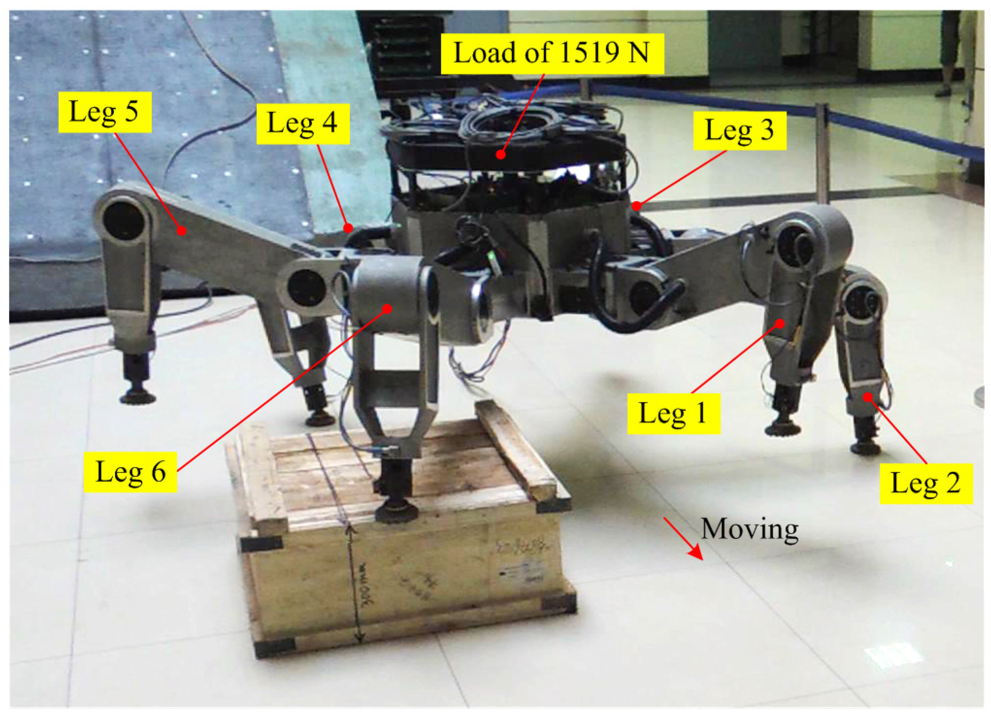
5. Applications and Experiments

Based on our previous research results and the engineering technical indexes of the robot, a prototype of an electrically driven large-load-ratio six-legged robot is developed. The gait planning strategies are written in C++ language and downloaded to the system of the robot. Due to the same method of gait planning for the tripod gait, quadrangular gait, and pentagon gait, the tripod gait is only employed to verify the reasonableness of the gait planning strategies. Then, the experiments of the walking speed and surmounting obstacle are respectively performed. To check the reasonableness of the gait planning strategies, the robot uses 0.4 times the maximum walking speed as the goal speed to perform the walking speed test. The reasonableness of the gait planning can be verified when the robot achieves the above-stated walking speed.
The ant-typed tripod gait is selected for the experiment of walking speed for the large-load-ratio six-legged robot. Then, the body of the robot carries the load of 1519 N. The movement time (TM) is set as 100 ms in the programmable multi-axis controller (PMAC). The support distance of the leg i is set as 0.2 m in the support phase. Hence, the theoretical walking distance should be 2vmaxT/5 for the large-load-ratio six-legged robot in a gait period. The experiment using the walking speed 2vmax/5 under a load of 1519 N is shown in Figure 7. Based on the range sensor installed in the robot body, the walking distance lb of the robot can be obtained with the change of time t. Then, the curve of walking speed is drawn and is shown in Figure 7.
Based on Figure 7, the actual walking speed of the robot can be calculated though the walking distance lb and time t. Then, the contrastive analysis is implemented between the actual walking speed of the robot and the theoretical walking speed 2vmax/5. The contrastive result shows that the data are both the same. The reasonableness of the gait planning is verified for the large-load-ratio six-legged robot.
Based on Figure 3 and Figure 7, it is concluded that legs 1 and 2 can fully reflect the characteristics of the support phase and transfer phase when the large-load-ratio six-legged robot walks using the ant-type tripod gait. According to the PMAC motion control card, the pulse number curves of the servo motors are respectively obtained for the abductor joints, hip joints, and knee joints of legs 1 and 2; they are shown in Figure 8. In Figure 8, we can find that the pulse number curves of the servo motors are smooth. Hence, we conclude that the ride comfort of the rotation joints can be demonstrated. The correctness of the solution is verified in the analyses of the forward and inverse kinematics of the robot. In Figure 8, the minus sign only indicates that the steering of the servo motor is opposite to the specified positive steering.
The prototype of the large-load-ratio six-legged robot employs the tripod gait to stride across the vertical obstacle under the load of 1519 N. The experiment of the surmounting obstacle is shown in Figure 9. The parts of the walking parameters are set for the robot prototype. The height of the body is defined as 0.6 m. The maximum swing height hT-max is set as 0.34 m. The step pitch s is 0.3 m. Leg 4 and leg 6 trample on the vertical obstacle. Other legs do not trample on the obstacle. Then, it is found that the large-load-ratio six-legged robot can stride across the vertical obstacle under the tripod gait. The impact phenomenon does not appear between the foot and the ground. Hence, the rationality of the gait planning can be confirmed for the large-load-ratio six-legged robot.

6. Conclusions

In this article, the strategies of gait planning are presented for the electrically driven large-load-ratio six-legged robot. To make the robot maintain the characteristics of universal walking, the body structure of the robot is designed as a regular polygon. The six legs are evenly distributed around the body of the robot. The conventional gaits and walking modes are respectively designed based on the configuration of the robot. The higher-stable swing sequences of legs and typical walking modes are obtained. The D-H model of leg i is established. The analyses of the forward and inverse kinematics are implemented. The mathematical expressions of the rotation angles are respectively gained for the abductor joint, hip joint, and knee joint.
To reduce the impact force between the foot and the ground, a buffer device is installed at the end of shin. The initial lift height of the leg is brought into the gait planning when the support phase changes to the transfer phase. The mathematical models of the foot trajectories are respectively established for the support phase and transfer phase. Based on the previous research results, a prototype of the electrically driven large-load-ratio six-legged robot is developed. Experiments with the robot are conducted regarding the walking speed and surmounting obstacle. The experimental results show that the gait planning strategies are reasonable and can effectively reduce the impact force between the foot and the ground. The gait planning strategies in this article can provide a reference for large-load-ratio multi-legged robots.

Acknowledgments

This project is supported by the National Natural Science Foundation of China (Grant No. 51505335) and the National Natural Science Foundation of China (Grant No. 51275106).

Author Contributions

Hong-Chao Zhuang conceived the topic and developed the equations; Hong-Chao Zhuang, Hai-Bo Gao, and Zong-Quan Deng performed the applications and experiments; and Hong-Chao Zhuang wrote the article.

Conflicts of Interest

The authors declare no conflict of interest.

References

  1. Raibert, M.; Blankespoor, K.; Nelson, G.; Playter, R.; the BigDog Team. BigDog, the rough-terrain quadruped robot. In Proceedings of the 17th World Congress on the International Federation of Automatic Control, Seoul, Korea, 6–11 July 2008; pp. 10822–10825.
  2. Playter, R.; Buehler, M.; Raibert, M. BigDog. In Proceedings of the International Society for Optical Engineering, Bellingham, WA, USA, 1–6 January 2006.
  3. Irawan, A.; Nonami, K. Optimal impedance control based on body inertia for a hydraulically driven hexapod robot walking on uneven and extremely soft terrain. J. Field Robot. 2011, 28, 690–713. [Google Scholar] [CrossRef]
  4. Irawan, A.; Nonami, K.; Ohroku, H.; Akutsu, Y.; Imamura, S. Adaptive impedance control with compliant body balance for hydraulically driven hexapod robot. J. Syst. Des. Dyn. 2011, 5, 893–908. [Google Scholar] [CrossRef]
  5. SunSpiral, V.; Wheeler, D.W.; Chavez-Clemente, D.; Mittman, D. Development and field testing of the footfall planning system for the ATHLETE robots. J. Field Robot. 2012, 29, 483–505. [Google Scholar] [CrossRef]
  6. Wilcox, B.H.; Litwin, T.E.; Biesiadecki, J.J.; Matthews, J.; Heverly, M.; Morrison, J.; Townsend, J.; Ahmad, N.; Sirota, A.; Cooper, B. ATHLETE: A cargo handling and manipulation robot for the moon. J. Field Robot. 2007, 24, 421–434. [Google Scholar] [CrossRef]
  7. Erden, M.S.; Leblebicioğlu, K. Free gait generation with reinforcement learning for a six-legged robot. Robot. Auton. Syst. 2008, 56, 199–212. [Google Scholar] [CrossRef]
  8. Erden, M.S.; Leblebicioǧlu, K. Analysis of wave gaits for energy efficiency. Auton. Robot. 2007, 23, 213–230. [Google Scholar]
  9. Ishikawa, T.; Makino, K.; Imani, J.; Ohyama, Y. Gait motion planning for a six legged robot based on the associatron. J. Adv. Comput. Intell. Intell. Inform. 2014, 18, 135–139. [Google Scholar]
  10. Estremera, J.; Cobano, J.A.; de Santos, P.G. Continuous free–crab gaits for hexapod robots on a natural terrain with forbidden zones: An application to humanitarian demining. Robot. Auton. Syst. 2010, 58, 700–711. [Google Scholar] [CrossRef] [Green Version]
  11. Satzinger, B.W.; Lau, C.; Byl, M.; Byl, K. Tractable locomotion planning for RoboSimian. Int. J. Robot. Res. 2015, 34, 1541–1558. [Google Scholar] [CrossRef]
  12. Fielding, M.R.; Dunlop, G.R. Omnidirectional hexapod walking and efficient gaits using restrictedness. Int. J. Robot. Res. 2004, 23, 1105–1110. [Google Scholar] [CrossRef]
  13. Tedeschi, F.; Carbone, G. Hexapod walking robot locomotion. In Motion and Operation Planning of Robotic Systems, 1st ed.; Carbone, G., Gomez-Bravo, F., Eds.; Springer: Cham, Switzerland, 2015; Volume 29, pp. 439–468. [Google Scholar]
  14. Tedeschi, F.; Carbone, G. Design of hexapod walking robots: Background and challenges. In Handbook of Research on Advancements in Robotics and Mechatronics, 1st ed.; Habib, M.K., Ed.; Idea Group: Hershey, PA, USA, 2014; Volume 2, pp. 527–566. [Google Scholar]
  15. Sadati, N.; Dumont, G.A.; Hamed, K.A.; Gruver, W.A. Hybrid Control and Motion Planning of Dynamical Legged Locomotion, 1st ed.; Wiley-IEEE Press: Hoboken, NJ, USA, 2012; pp. 95–217. [Google Scholar]
  16. Zhuang, H.C.; Gao, H.B.; Deng, Z.Q.; Ding, L.; Liu, Z. Method for analyzing articulated rotating speeds of heavy-duty six-legged robot. J. Mech. Eng. 2013, 49, 44–52. [Google Scholar] [CrossRef]
  17. Gao, H.B.; Zhuang, H.C.; Li, Z.G.; Deng, Z.Q.; Ding, L.; Liu, Z. Optimization and experimental research on a new-type short cylindrical cup-shaped harmonic reducer. J. Cent. South Univ. Technol. 2012, 19, 1869–1882. [Google Scholar] [CrossRef]
  18. Zhuang, H.C.; Gao, H.B.; Deng, Z.Q.; Ding, L.; Liu, Z. A review of heavy-duty legged robots. Sci. China Technol. Sci. 2014, 57, 298–314. [Google Scholar] [CrossRef]
  19. Zhuang, H.C.; Gao, H.B.; Deng, Z.Q. Analysis method of articulated torque of heavy-duty six-legged robot under its quadrangular gait. Appl. Sci. 2016, 6, 1–21. [Google Scholar] [CrossRef]
  20. Jun, N.S. Legged insects select the optimal locomotor pattern based on the energetic cost. Biol. Cybern. 2000, 83, 435–442. [Google Scholar]
  21. Lin, B.S.; Song, S.M. Dynamic modeling, stability, and energy efficiency of a quadrupedal walking machine. J. Robot. Syst. 2001, 18, 657–670. [Google Scholar] [CrossRef]
Figure 1. Electrically driven large-load-ratio six-legged robot: (a) schematic diagram of the mechanism; and (b) top view of the mechanism.
Applsci 07 00296 g001
Figure 2. Structure of the leg of the large-load-ratio six-legged robot.
Applsci 07 00296 g002
Figure 3. Four kinds of typical walking modes for the large-load-ratio six-legged robot: (a) crab type; (b) ant type; (c) crab–ant mixed type I; and (d) crab–ant mixed type II.
Applsci 07 00296 g003
Figure 4. D-H (Denavit-Hartenberg) model of leg i of the large-load-ratio six-legged robot.
Applsci 07 00296 g004
Figure 5. Posture of leg i of the large-load-ratio six-legged robot.
Applsci 07 00296 g005
Figure 6. Feet trajectories of leg i in the tripod gait: (a) transfer phase; and (b) support phase.
Applsci 07 00296 g006
Figure 7. Experiment of walking speed 2vmax/5 under a load of 1519 N: (a) experiment of the walking speed of 2vmax/5 of the prototype; and (b) curve of walking speed for the robot body.
Applsci 07 00296 g007
Figure 8. Pulse number curves of servo motors for abductor joints, hip joints, and knee joints: (a) leg 1; and (b) leg 2.
Applsci 07 00296 g008
Figure 9. Experiment of surmounting an obstacle under a load of 1519 N.
Applsci 07 00296 g009
Table 1. Parts of the gait parameters of the large-load-ratio six-legged robot.
Duty Ratio βRNumber (u) of Legs in Support Phase GaitSupport Time (Ts) between Legs of Support Phase Walking Speed vR
βR = 1/23Tripod GaitEqualityvR = 2s/T
βR = 2/34Quadrangular GaitEqualityvR = 3s/2T
βR = 5/65Pentagon GaitEqualityvR = 6s/5T
βR = 16Stationary State Equality0
Table 2. Higher-stable swing sequences of legs in the quadrangular gait.
No.Phase1/3 Gait Legs2/3 Gait Legs3/3 Gait LegsNo.Phase1/3 Gait Legs2/3 Gait Legs3/3 Gait Legs
1Transfer2, 53, 61, 410Transfer1, 52, 43, 6
Support1, 3, 4, 61, 2, 4, 52, 3, 5, 6Support2, 3, 4, 61, 3, 5, 61, 2, 4, 5
2Transfer2, 43, 61, 511Transfer1, 53, 62, 4
Support1, 3, 5, 61, 2, 4, 52, 3, 4, 6Support2, 3, 4, 61, 2, 4, 51, 3, 5, 6
3Transfer2, 41, 53, 612Transfer1, 42, 53, 6
Support1, 3, 5, 62, 3, 4, 61, 2, 4, 5Support2, 3, 5, 61, 3, 4, 61, 2, 4, 5
4Transfer3, 62, 51, 413Transfer1, 42, 63, 5
Support1, 2, 4, 51, 3, 4, 62, 3, 5, 6Support2, 3, 5, 61, 3, 4, 51, 2, 4, 6
5Transfer3, 62, 41, 514Transfer1, 43, 62, 5
Support1, 2, 4, 51, 3, 5, 62, 3, 4, 6Support2, 3, 5, 61, 2, 4, 51, 3, 4, 6
6Transfer3, 61, 52, 415Transfer1, 43, 52, 6
Support1, 2, 4, 52, 3, 4, 61, 3, 5, 6Support2, 3, 5, 61, 2, 4, 61, 3, 4, 5
7Transfer3, 61, 42, 516Transfer2, 63, 51, 4
Support1, 2, 4, 52, 3, 5, 61, 3, 4, 6Support1, 3, 4, 51, 2, 4, 62, 3, 5, 6
8Transfer3, 51, 42, 617Transfer2, 61, 43, 5
Support1, 2, 4, 62, 3, 5, 61, 3, 4, 5Support1, 3, 4, 52, 3, 5, 61, 2, 4, 6
9Transfer3, 52, 61, 418Transfer2, 51, 43, 6
Support1, 2, 4, 61, 3, 4, 52, 3, 5, 6Support1, 3, 4, 62, 3, 5, 61, 2, 4, 5
Table 3. Contributions from the joints to the walking speed of the robot. NC: non-contribution; AC: auxiliary contribution; MC: main contribution.
Walking Wayθi Changing form 0° to 60°θi = 60°
Legs 1, 3, 4, and 6Legs 2 and 5Legs 1, 3, 4, and 6Legs 2 and 5
AiHi and KiAiHi and KiAiHi, KiAiHi, Ki
Crab typeFrom NC to MC vRForm MC to AC vRNC vRMC vR
Ant typeMC vRAC vRMC vRAC vR
Crab–ant mixed type IMC vRAC vRNC vRMC vR
Crab–ant mixed type IIMC vRAC vRMC vRAC vR
Table 4. Parameters of the D-H model of leg i.
Joint jLinkage Length
a j 1 ( i ) (mm)
Torsion Angle of Link
α j 1 ( i ) (deg)
Linkage Offset
d j ( i ) (mm)
Rotation Angle of Link
θ j ( i ) (deg)
100θi
2lc90°0βi
3lt0γi

