
Collision Avoidance for Cooperative UAVs with Rolling Optimization Algorithm Based on Predictive State Space

Information System and Management College, National University of Defense Technology, Changsha 410073, China
*
Author to whom correspondence should be addressed.
Appl. Sci. 2017, 7(4), 329; https://doi.org/10.3390/app7040329
Submission received: 23 December 2016
/
Revised: 17 March 2017
/
Accepted: 20 March 2017
/
Published: 28 March 2017
Abstract
:Unmanned Aerial Vehicles (UAVs) have recently received notable attention because of their wide range of applications in urban civilian use and in warfare. With air traffic densities increasing, it is more and more important for UAVs to be able to predict and avoid collisions. The main goal of this research effort is to adjust real-time trajectories for cooperative UAVs to avoid collisions in three-dimensional airspace. To explore potential collisions, predictive state space is utilized to present the waypoints of UAVs in the upcoming situations, which makes the proposed method generate the initial collision-free trajectories satisfying the necessary constraints in a short time. Further, a rolling optimization algorithm (ROA) can improve the initial waypoints, minimizing its total distance. Several scenarios are illustrated to verify the proposed algorithm, and the results show that our algorithm can generate initial collision-free trajectories more efficiently than other methods in the common airspace.
1. Introduction
Because of their low-cost, high-autonomy, super-flexibility, and especially absence of human risk, unmanned aerial vehicles (UAVs) have the potential to offer various capabilities for military and civilian applications. Recently, with the advances of dynamics [1,2], navigation [3,4], and sensors [5,6], more civilian applications have been realized for UAVs, such as surveillance [7,8], aerial photography [9,10], search and rescue [11,12], and others. For all of these applications with multiple UAVs, one critical technical problem is that the UAVs may collide with each other in the increasingly dense airspace. Although UAV collision does not cause the loss of human life, it still causes economic loss and seriously affects the task that UAVs are undertaking. Besides, with the occupancy of the airspace being denser, the ground station-based air traffic control cannot be sufficient to track every aircraft. As a result, it is essential to have an automatic UAV collision avoidance strategy to prevent unnecessary loss and guarantee the success rate of missions.
Generally, for conventional flight, Traffic Alert and Collision Avoidance System (TCAS) or Global Positioning System (GPS)-based traffic display system is facilitated in manned aircraft to detect and alert possible collision in the near future. When two aircrafts are predicted to reach a certain distance, the system would alert the pilots to maneuver to avoid the collision. In terms of UAVs, relevant research is growing at a fantastic speed to realize the purpose of “free flight” [13], which has been the main issue for UAV mission implementation. Normally, assumptions that cooperative UAVs can communicate their positions, speed, heading, waypoints, and proposed trajectories are allowed [14,15]. With the airspace density increasing, centralized methods are more computationally expensive to solve the UAVs’ collision avoidance problem. Some proposed approaches change the UAVs’ speed in a centralized way to avoid the predicted collision [16,17]. However, the velocity amendment of the UAV is usually limited. Therefore, UAVs may still collide with each other if only velocity is adjusted. Based on the consideration above, some researchers adjust the heading direction of UAVs and keep a constant velocity to avoid collision [15,18]. UAV collision avoidance methods are proposed by varying heading, velocity, or both [14,19,20]. However, the method sets the UAVs at constant altitude, which limits the practical use of the method.
When it comes to methodology, many laws in other fields have been applied to avoid collision among UAVs. Methods based on potential field have been widely proposed [21,22], while the idea of genetic methods [18,19] is also popular to avoid collision. The proportional navigation guidance law is used to solve the problem [23], which is one of the most-used strategies for missile engagement scenarios. Other strategies solving the problem are based on optimization algorithms, such as dynamic programming [24], Lyapunov Method [20], Markov Decision Process [25], radio signal strengths [26], rapidly-exploring random tree [27], and so on.
In this paper, a 3D conflict avoidance problem for cooperative multiple UAVs sharing airspace is proposed. In the particular local airspace, it is assumed that the initial trajectory (a sequence of waypoints), real-time position, heading, and velocity of each UAV are shared as the sensors in the UAVs scan the environment at a fixed interval. Considering that conflict avoidance problem among UAVs is non-deterministic polynomial-time hard (NP-hard) [28], we transfer it to be discrete by sampling, which has been proven to have better performance in solving NP-hard problems [29]. We also consider the heading and position of each UAV at the next interval as the state condition. The rolling optimization algorithm (ROA) we propose predicts whether a collision may occur. If there are no potential collisions, UAVs continue flying as planned; otherwise, the algorithm provides the maneuver to avoid collision and updates the trajectory. The goal of this proposed algorithm is to minimize flying distance when collisions are avoided. It detects and avoids collisions with each sensor scan, which is the main reason we call the process of optimization “rolling”.
This paper is organized as follows. First, the problem formulation and modeling are stated. Later, the proposed rolling optimization algorithm (ROA) is introduced. Therein, collision prediction and avoidance maneuvers are described in detail. This is followed by various collision scenarios, which are carried out and demonstrated to verify the effectiveness of the proposed algorithm. Finally, a brief summary of the research is presented.
2. Problem Formulation and Modeling
In this section, we introduce the formulation of the problem. Based on some valid assumptions, the mathematical modeling of the problem is constructed.
2.1. Problem Formulation and Presentation
The general scenario is that several UAVs are flying from different bases to their respective destinations. However, collisions may occur if all of them choose the shortest path. For safety reasons, any pair of UAVs should keep the minimum separation, which is usually greater than a constant (safe distance). To minimize the cost of the total flight distance, the solution only considers the intermediate waypoints, which are added in the initial trajectory because of collision avoidance. Thus, after a potential collision is detected, trajectories (waypoints) of UAVs should be adjusted so that their trajectories satisfy the collision-free requirement.
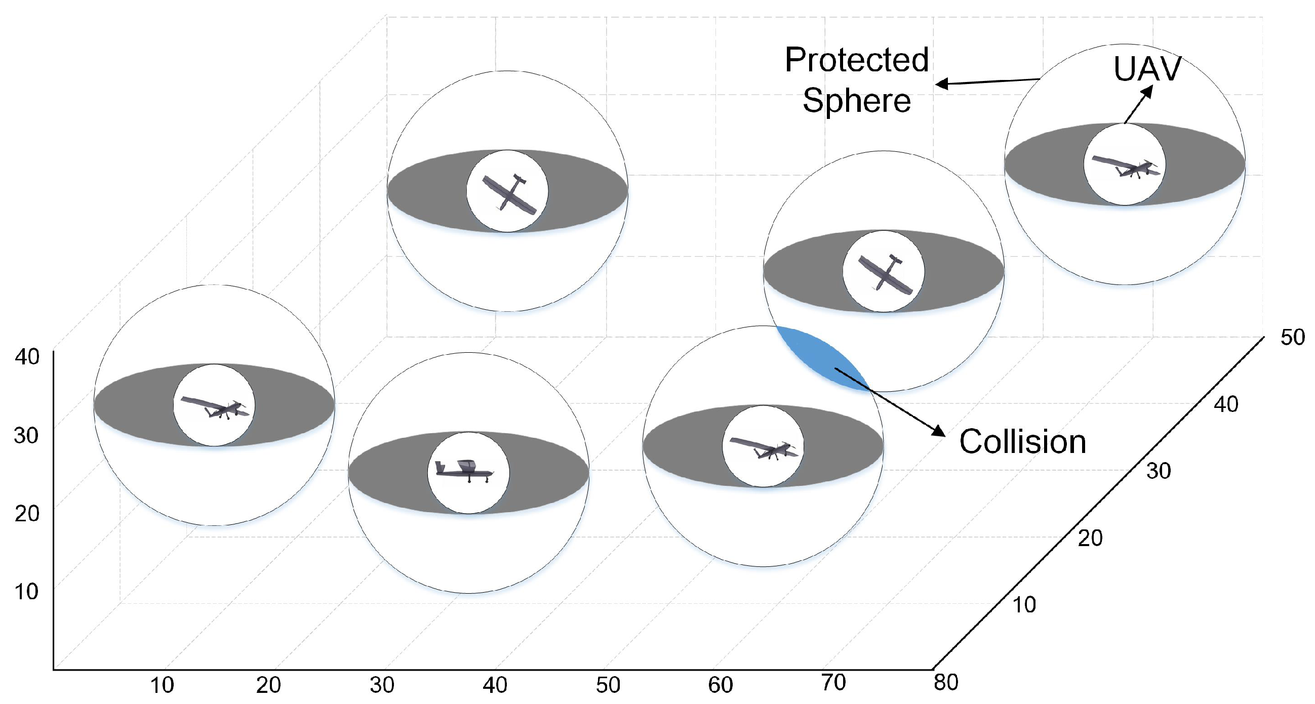
A typical scenario is presented in Figure 1. In the shared airspace, there are six cooperative UAVs performing their tasks. The protected area is represented by the sphere outside the UAVs. The radius of the sphere is slightly greater than the safety distance, which means UAVs would collide when their protected spheres interlace. It is worth noting that the volume of the protected area is relevant to the size of the aircraft.
As a result, the information needed to solve the problem includes the planned trajectories of UAVs with their initial locations and goal destinations.
2.2. Grid Model and State Space
In this paper, towards the aim of discretization, the common airspace is divided into cubic cells called the grid model. The reason we use cubic cells rather than other shapes is that it is simpler to locate the position and calculate the distance between UAVs.
This is not the first use of the grid model in this field. In [30], a trajectory is parametrized by the number of cells that the UAV passes through with entrance and departure time. The size of cells is a parameter. Collision is defined as being when two UAVs lay in the same cell at the same time. Alejo et al. improved the collision model, considering the UAVs in the neighboring cells [31]. These models set the size of cubic cells as a large value, which is much greater than the radius of the protected area of the UAVs. However, waypoints of each UAV are recorded roughly in this way. In this paper, we consider a small value as the size of cubic cells, which makes the results more accurate. Then, the waypoints of UAVs can be represented as points in the coordinate.
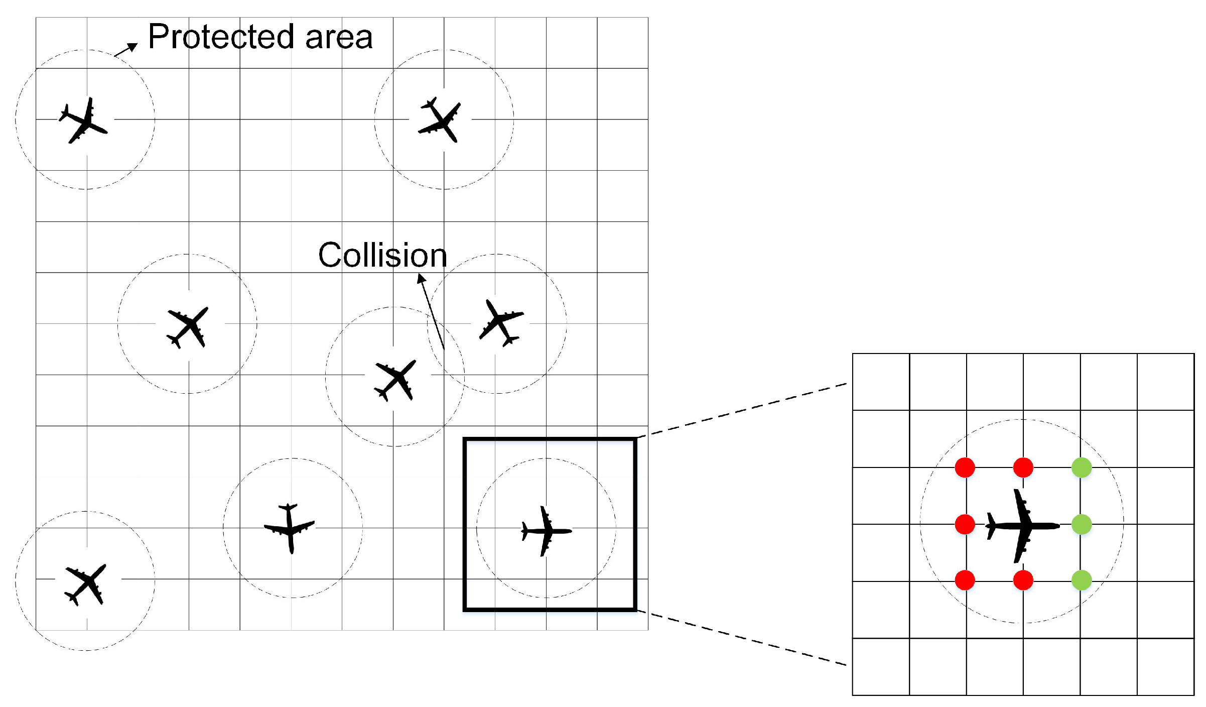
The top view of the encoded airspace is presented in Figure 2, and a 2D example of state space is illustrated. State space describes all the possible future states in the next intervals. When a UAV flies horizontally, the degree it can turn is limited in the fixed interval. In this paper, we set the degree as no more than 45 degrees. Therefore, on the right side of Figure 2, red points are not allowed for UAVs to reach, while only green points are possible waypoints in the next interval for UAVs. Thus, in 2D airspace, one UAV has three choices for the next move, and N UAVs would have viable states in the next interval, which has formed a state space. In this paper, 3D state space of multiple UAVs is considered, which is much more complicated than the 2D state space.
3. Rolling Optimization Algorithm
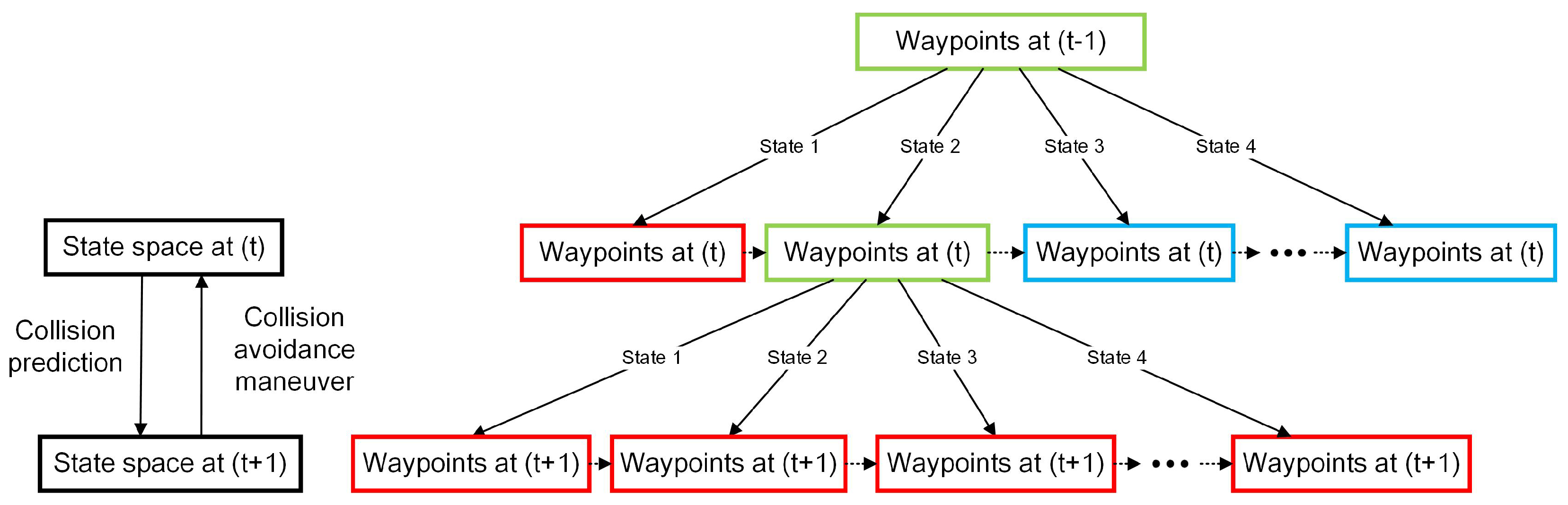
In this section, we introduce the ROA based on state space. The conceptual model is shown in Figure 3. The algorithm predicts possible collisions when the planned trajectories of all the UAVs are shared. If there are no collisions detected in the planned trajectories, the UAVs would fly as planned; on the other hand, the algorithm would provide a collision avoidance maneuver and update the UAV trajectories.
3.1. Objective Function
For the i- UAV, the position at time is shown as in Equation (1). In the equation, denotes the position of the i- UAV at time t, while describes its velocity. The sampling interval is .
Because we used a grid model for discretization, the position p and velocity v are represented by column vectors, as shown in Equation (2). Furthermore, items in the is limited to be −1, 0, or 1 to guarantee that UAVs stay in the crossing points of the grid model.
The best trajectories of multiple UAVs have the shortest flying distance, satisfying the collision-free constraint. In this paper, the total flying distance of all the UAVs is considered as the objective function. The mathematical expression is shown in Equation (3). Therein, denotes the number of intervals that the i- UAV spends from the base to the destination, while N is the number of UAVs.
3.2. Constraints
For the aim of UAVs performing tasks without collision, we introduce three constraints for the trajectories of UAVs in the sector.
First, the UAVs have to satisfy the rule made in the state space; i.e., the absolute value of degree between adjacent heading directions is no more than 45 degrees. The mathematical expression is shown in Equation (4). In practice, this constraint can be adapted according to the mechanical properties of UAVs.
The second constraint is that the absolute value of degrees between UAV heading and the direction from the current position to the destination is no more than 90 degrees, as Equation (5) shows. The constraint guarantees that UAVs always head to the destination. In the equation, denotes the goal destination of the i- UAV.
The last constraint requires that the distance between any two UAVs is no more than the radius of the protected sphere, as shown in Equation (6). The constraint ensures that collisions are avoided in the proposed trajectories. In the equation, R stands for the radius of the protected sphere of UAVs.
3.3. Trajectory Generation
During UAV flight, the algorithm generates a real-time collision-free trajectory for the next several intervals by predicting and avoiding possible collisions. The 3D state space is utilized, which makes the situation more complicated than that in 2D. One scenario is presented in Figure 4. In the figure, the UAV with solid lines represents the UAV’s current position, while the UAV with dashed lines shows the last position. The gray triangle is forbidden for UAVs because it violates the turn degree limitation, which is that in this paper the degree between adjacent heading directions is no more than 45 degrees. On the contrary, the black rectangle represents the allowed position of the UAV in the subsequent move. Therefore, N UAVs would have possible states in the ensuing interval if the limitation of heading direction change degree is not considered. In this paper, the state space has removed a large number of possible waypoints, and lowered the computation complexity greatly. For the possible feasible waypoints, we set a weight for each position, which is relevant to three factors.
The first factor is the distance between the upcoming possible position and the destination point. The farther the distance is, the lower the weight of the candidate point would be. The factor is calculated as shown in Equation (7). Therein, the numerator is considered to adjust the weight of the factor. calculate the Euclidean distance between vectors a and b.
The second factor is the angle between the possible heading direction and direction from the possible point to the destination point. The degree describes the level of deviation of the UAV from the shortest distance path. It is shown in Equation (8). The 0.1 in the denominator is set in case the angle 0 would make the factor infinite.
The last factor is the eigenvalue of the crossing points in the grid model. The initial eigenvalue of each crossing point is set to be 1. Eigenvalues of points would change with the generation of UAVs’ trajectories. Eigenvalue is the key information in ROA, and will be introduced later.
Based on the three factors above, the weight for each candidate point is determined as in Equation (9). The weight of each point depends on not only the distance, but also the angle by which the UAV has deviated from the planned path. stands for the information of the crossing points.
According to the weights for each candidate position, the roulette method is used to determine the position of the UAV in the next interval. The reason we use the roulette method is that although it is more likely for the greatest value position to be the next waypoint, it still can be other points. It would help the algorithm solve the problem of getting into the local optimization solution to some extent.
3.4. Collision Prediction and Avoidance Maneuver
After UAVs use the roulette method to determine their positions in the next interval, the algorithm automatically detects whether the next state would cause collisions. That is, to detect whether the distance of any two UAVs is no more than the radius of the protected sphere. If the state satisfies the collision-free condition, the algorithm continues. Otherwise the chosen state would cause collisions, and the algorithm would set the weight of each waypoint in the collision state as 0. Then, the state in the next interval is reselected until the state can avoid collisions. If all the states in the state space cannot avoid collisions. The algorithm would return to the last state and reselect the current UAV positions.
The process of collision prediction and avoidance maneuver is illustrated in Figure 5. The green rectangle represents the waypoints that would not cause any collisions, and the red rectangle represents waypoints which cannot avoid collisions. The blue rectangle trajectory has not been tested. At the interval of t, state 1 is not collision-free. Therefore, state 2 is selected to be the waypoints at interval t. However, the collision prediction process finds that all the states in the state space expanded by state 2 at t would cause collisions. As a result, the collision avoidance maneuver would force the state 2 at t to be discarded, and select state 3 at t as the waypoints. The process above loops as the algorithm continues.
3.5. Rolling Optimization
The two sections above have introduced how collision-free trajectories are generated. In this section, we introduce the rolling optimization method to generate shorter trajectories with the condition of being collision-free.
The key of the rolling optimization is the third factor (eigenvalue) influencing the weight for each candidate waypoint in the next move for UAVs. In the grid model, each crossing point has an eigenvalue. If a crossing point is selected as a waypoint in a trajectory, its eigenvalue should be updated in two ways. The local update represents that the eigenvalue of the point should be decreased after it is chosen to be one waypoint in the trajectory of the UAV. For the aim of global search, the local update indirectly increases the probability of other candidate positions. The mathematical expression of the iteration is shown in Equation (10). Therein, denotes the eigenvalue of the location , while represents the decreasing coefficient.
A global update would happen when several searched trajectories are determined in an iteration. The shortest path in the searched trajectories is selected, and all the waypoints are updated in the shortest trajectory. Equation (11) calculates the update process of the eigenvalue at location after the iteration. Therein, denotes the update coefficient. describes the update value, and the mathematical expression is shown in Equation (12). In the equation, denotes the distance of the shortest trajectory, and is a coefficient adjusting the update value.
The update of candidate waypoint eigenvalues makes the short distance waypoints have more probability to be selected. What is more, it helps the algorithm get rid of local optimal values.
3.6. Programming Steps
The pseudo-code of the proposed algorithm is shown in Algorithm 1. Therein, the collision prediction process and avoidance maneuver are in bold. In the beginning, the algorithm searches the candidate points randomly. With the iteration number increasing, the eigenvalues tend to be stable. Shorter trajectories of UAVs are assigned to more probability. That is how the ROA works.
| Algorithm 1: Pseudo-code of ROA |
 |
4. Simulation and Results
This section describes the results obtained from the proposed ROA. Simulation of all the following scenarios has been accomplished with known UAV start positions and destination positions. What is more, UAVs are assumed to be heading to the destination along a straight line from their start points in the grid model. According to [32], the minimum distance is 5 nmi (about 9.26 km). Considering the deviation and fine tuning of UAVs in reality, we set the radius of the protected sphere to be greater (10 km). Table 1 shows some variable values applied in the following scenarios. Therein, R denotes the safety distance of UAVs, which is a fixed value for a certain UAV; are three variables affecting the weight for candidate points for the UAV in the next move, explained, respectively, in Equations (7), (8), and (12); is the decreasing coefficient of eigenvalue, listed in Equation (10), and the aim is to decrease the eigenvalue in the current best path so that the algorithm can get rid of local optimal value; is the update coefficient of eigenvalue, listed in Equation (11), which is expected to adjust the affection of the current best path. After numerical experiments, we find that the choices of the variables depend on the specific task, and only affect the flying distance and computation duration, but do not lead to collisions. To clearly describe the performance of the ROA, the choice of variable values is just a random case.
4.1. Scenario 1: Pairwise Case
For the pairwise case, the initial position and the destination are shown in Table 2. All the results are illustrated in Figure 6.
We set the number of random searches in one iteration as 10, and the number of iterations as 5000. The expected time to detect collisions is 2 . Therein, denotes the time it takes for a UAV to fly across a cubic cell. That is, the experiment can detect collisions two steps ahead. The initial collision-free trajectory and the 5000th collision-free trajectory are shown in Figure 6a,b. The total distance is 894.77 and 759.56, respectively.
Figure 6c demonstrates the change of total distance with the iteration number. We find that the proposed algorithm can get effectively rid of the local optimization point. The total distance tends to be stable after 3000 iterations.
Relative distance in the best result with fixed intervals is illustrated in Figure 6d. As expected, the shortest distance between two UAVs is larger than the radius of the protected sphere, which is 10 in the scenario.
4.2. Scenario 2: Six-UAVs Case
To validate the efficacy of our proposed algorithm for a more complicated scenario, six UAVs in a common airspace implementing tasks are simulated. The initial position and the destination are shown in Table 3. All the results are presented in Figure 7.
We set the number of random searches in one iteration as 10, and the number of iterations as 5000. The expected time to detect a collision is 2 . The initial collision-free trajectory and the 5000th collision-free trajectory are shown in Figure 7a,b. The total distance is 2553.89 and 2215.71, respectively.
Figure 7c demonstrates the change of total distance with the iteration number. We can find that the proposed algorithm can get rid of local optimization point effectively. The total distance tends to be stable after 4500 iterations.
Relative distance in the best result with fixed intervals is illustrated in Figure 7d. As expected, the shortest distance between two UAVs is larger than the radius of the protected sphere, which is 10 in the scenario.
4.3. More Scenarios
We also conduct more experiments to verify the flexibility and efficiency of the ROA. Based on Scenario 2, we set the same six UAVs having fixed start points and destination points in this experiment. We also add other UAVs having random start points and destination points in the section. Other variables are the same as the scenarios above. We conduct the experiments with the number of UAVs ranging from 7 to 20. The algorithm could generate the collision-free trajectories for all cases. Table 4 lists all the cases and time spent during ten iterations. From the table, we can find that the computational cost of the ROA is acceptable.
4.4. Comparison with Other Methods
In this section, an index is set to evaluate different collision avoidance algorithms. In most cases, relevant methods can efficiently avoid the potential collision in UAV trajectories [23,27]. Generally, run duration depends not only on the efficiency of the algorithms, but also on the size of the map and velocity in the simulated scenarios. As a consequence, the index should remove the effects of the artificial settings and focus on the computation complexity of the methods. The index evaluating run duration of collision avoidance systems is shown in Equation 13. Therein, denotes the run duration of the collision avoidance algorithm; represents the total distance of UAVs in the simulated scenario of the method, while describes the average velocity of UAVs in the scenario of the system.
The results of the evaluation index are shown in Table 5. The comprised methods are the algorithms which are currently widely used and effective. “ROA1” is the result of one iteration with six UAVs, which can generate collision-free trajectories, though the total distance is longer. “ROA5000” shows the result of 5000 iterations. The result generates the collision-free waypoints with the shortest total distance. The evaluating indices of proportional navigation method and rapidly-exploring random tree method are between those of “ROA1” and “ROA5000”. Therefore, it is validated that our proposed algorithm can generate trajectories for multiple UAVs without any collisions, and can obtain optimized waypoints by rolling process.
5. Conclusions
In this paper, an efficient method of collision prediction and avoidance maneuvering is represented with a rolling optimization algorithm based on predictive state space. A team of cooperative and homogeneous UAVs is considered to fly in the common airspace, which is described by grid model, and the UAV waypoints are limited to be the crossing points among cubes. Under some restrictions, optimal trajectories with the shortest total trajectories of the UAVs involved are generated. The simulation results have validated the effectiveness of the proposed method.
The main contributions of this paper include:
- A novel and effective collision avoidance maneuver is presented, and the scenarios have validated the effectiveness of the proposed algorithm. The collision-free trajectories can be obtained in a short time, and performance of the better results depends on the run duration of the algorithm.
- The variables in the ROA can adjust freely according to the specific tasks.
- Predictive state space is used to reduce the dimension of the waypoints of UAVs in the next move, which has decreased the computation complexity greatly and improved the efficiency of the proposed algorithm.
- The rolling optimization algorithm makes good performance by getting rid of local optimal value of the objective function, obtaining better results as the algorithm continues.
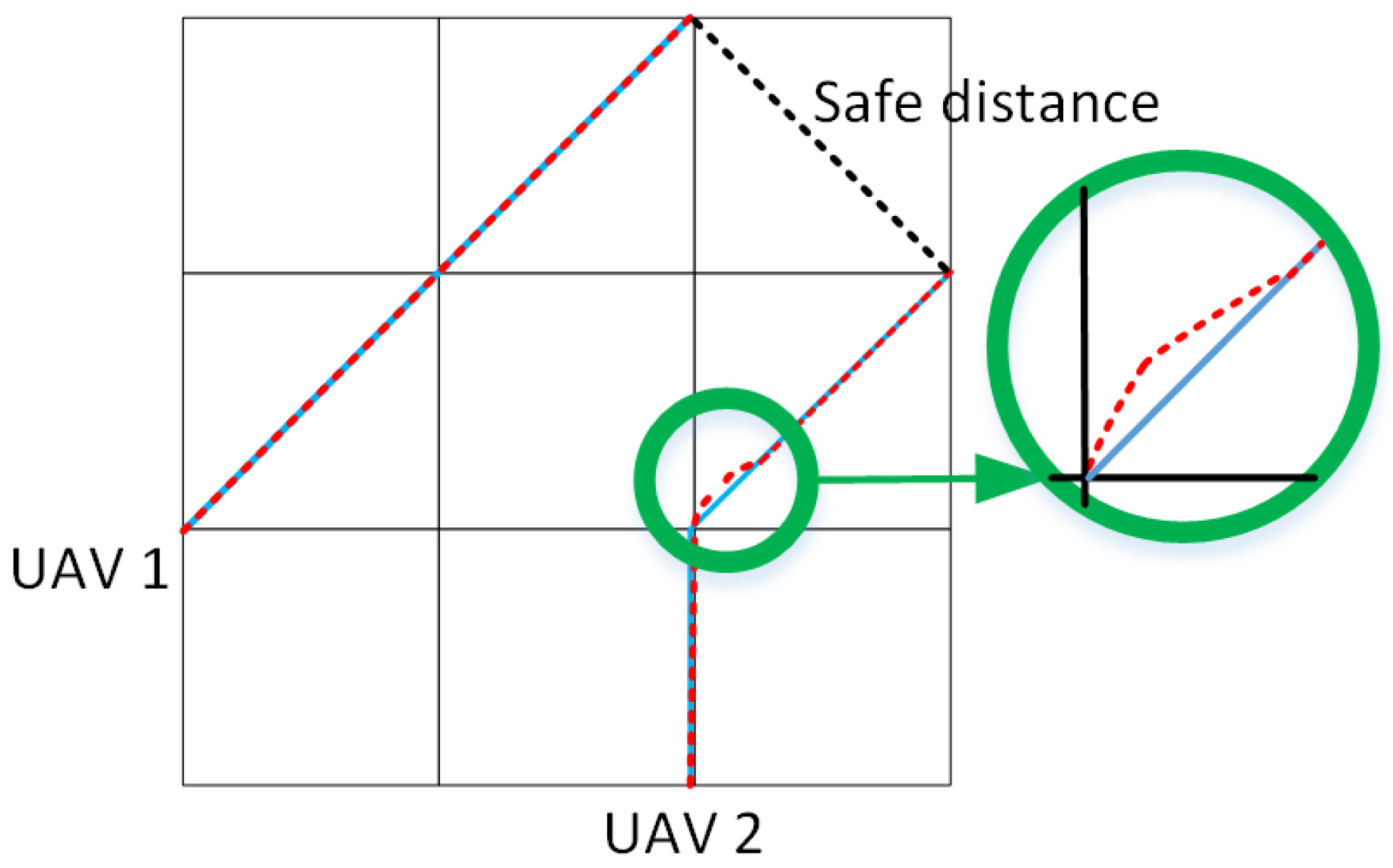
The main future work will consider the problem that real UAVs may make fine tuning adjustments when following the generated trajectories to cause potential collisions. A diagrammatic sketch is shown in Figure 8. In the figure, the blue solid line is the trajectories generated by ROA, and the red dashed line denotes the real trajectories of UAVs. The collision (distance shorter than the safe distance) might happen when the UAVs do not fly as planned. In the future work, we will research what the real trajectory of UAVs would be after the generated trajectory is received. What is more, we will research a trajectory smoothing algorithm to produce more robust trajectories for UAVs.
Acknowledgments
The authors disclosed receipt of the following financial support for the research, authorship, and/or publication of this article: This work was supported by the National Natural Science Foundation of China (71601181), and the State Key Laboratory of Management and Control for Complex Systems-Open Project (20160109).
Author Contributions
Tianyuan Yu and Jun Tang conceived and designed the experiments; Tianyuan Yu performed the experiments, Liang Bai and Songyang Lao helped in the experiment; Tianyuan Yu and Jun Tang analyzed the data; Tianyuan Yu and Jun Tang wrote the paper.
Conflicts of Interest
The authors declare no conflicts of interest.
References
- Caliskan, F.; Hajiyev, C. Active Fault-Tolerant Control of UAV Dynamics against Sensor-Actuator Failures. J. Aerosp. Eng. 2016, 29, 04016012. [Google Scholar] [CrossRef]
- Hajiyev, C.; Soken, H.E. Fault Tolerant Estimation of UAV Dynamics via Robust Adaptive Kalman Filter. In Complex Systems; Springer International Publishing: Berlin, Germany, 2016; pp. 369–394. [Google Scholar]
- Konovalenko, I.; Miller, A.; Miller, B.; Nikolaev, D.P. UAV navigation on the basis of the feature points detection on underlying surface. In Proceedings of the 29th European Conference on Modeling and Simulation (ECMS 2015), Albena (Varna), Bulgaria, 26–29 May 2015; pp. 26–29. [Google Scholar]
- Popov, A.; Miller, A.; Miller, B.; Stepanyan, K.; Konovalenko, I.; Sidorchuk, D.; Koptelov, I. UAV navigation on the basis of video sequences registered by onboard camera. In Proceedings of the 40th IITP RAS Interdisciplinary Conference and School, St. Petersburg, Russia, 25–30 September 2016. [Google Scholar]
- Rahimi, A.M.; Ruschel, R.; Manjunath, B.S. UAV Sensor Fusion With Latent-Dynamic Conditional Random Fields in Coronal Plane Estimation. In Proceedings of the IEEE Conference on Computer Vision and Pattern Recognition, Las Vegas, NV, USA, 27–30 June 2016; pp. 4527–4534. [Google Scholar]
- Clausen, P.; Rehak, M.; Skaloud, J. UAV Sensor Orientation with Pre-calibrated Redundant IMU/GNSS Observations: Preliminary Results. In Publikationen der Deutschen Gesellschaft für Photogrammetrie, Fernerkundung und Geoinformation (DGPF) eV; No. EPFL-CONF-220180; Deutsche Gesellschaft für Photogrammetrie, Fernerkundung und Geoinformation (DGPF) eV: Munich, Germany, 2016; Volume 25, pp. 26–33. [Google Scholar]
- Darrah, M.; Wilhelm, J.; Munasinghe, T.; Duling, K.; Yokum, S.; Sorton, E.; Rojas, J.; Wathen, M. A Flexible Genetic Algorithm System for Multi-UAV Surveillance: Algorithm and Flight Testing. Unmanned Syst. 2015, 3, 49–62. [Google Scholar] [CrossRef]
- Scherer, J.; Rinner, B. Persistent multi-UAV surveillance with energy and communication constraints[C]. In Proceedings of the 2016 IEEE International Conference on Automation Science and Engineering (CASE), Fort Worth, TX, USA, 21–24 August 2016; pp. 1225–1230. [Google Scholar]
- Turner, D.; Lucieer, A.; de Jong, S.M. Time series analysis of landslide dynamics using an unmanned aerial vehicle (UAV). Remote Sens. 2015, 7, 1736–1757. [Google Scholar] [CrossRef]
- Harwin, S.; Lucieer, A.; Osborn, J. The Impact of the Calibration Method on the Accuracy of Point Clouds Derived Using Unmanned Aerial Vehicle Multi-View Stereopsis. Remote Sens. 2015, 7, 11933–11953. [Google Scholar] [CrossRef]
- Kurdi, H.; How, J.; Bautista, G. Bio-Inspired Algorithm for Task Allocation in Multi-UAV Search and Rescue Missions. In Proceedings of the AIAA Guidance, Navigation, and Control Conference, San Diego, CA, USA, 4–8 January 2016; p. 1377. [Google Scholar]
- Beck, Z.; Teacy, L.; Rogers, A.; Jennings, N.R. Online planning for collaborative search and rescue by heterogeneous robot teams. In Proceedings of the 2016 International Conference on Autonomous Agents & Multiagent Systems, International Foundation for Autonomous Agents and Multiagent Systems, Singapore, 9–13 May 2016; pp. 1024–1033. [Google Scholar]
- Yang, L.C.; Kuchar, J.K. Prototype conflict alerting system for free flight. J. Guid. Control Dyn. 1997, 20, 768–773. [Google Scholar] [CrossRef]
- Rehmatullah, F.; Kelly, J. Vision-Based Collision Avoidance for Personal Aerial Vehicles Using Dynamic Potential Fields. In Proceedings of the 2015 12th Conference on Computer and Robot Vision (CRV), Halifax, NS, Canada, 3–5 January 2015; pp. 297–304. [Google Scholar]
- Lin, Y.; Saripalli, S. Collision avoidance for UAVs using reachable sets. In Proceedings of the 2015 International Conference on Unmanned Aircraft Systems (ICUAS), Denver, CO, USA, 9–12 June 2015; pp. 226–235. [Google Scholar]
- Alejo, D.; Conde, R.; Cobano, J.A.; Ollero, A. Multi-UAV collision avoidance with separation assurance under uncertainties. In Proceedings of the IEEE International Conference on Mechatronics, Malaga, Spain, 14–17 April 2009; pp. 1–6. [Google Scholar]
- Vela, A.; Solak, S.; Singhose, W.E.; Clarke, J.P. A mixed integer program for flight-level assignment and speed control for conflict resolution. In Proceedings of the Joint 48th IEEE Conference on Decision and Control and 28th Chinese Control Conference, Shanghai, China, 16–18 December 2009; pp. 5219–5226. [Google Scholar]
- Alejo, D.; Cobano, J.A.; Heredia, G.; Ollero, A. An Efficient Method for Multi-UAV Conflict Detection and Resolution Under Uncertainties. In Robot 2015: Second Iberian Robotics Conference; Springer International Publishing: Berlin, Germany, 2016; pp. 635–647. [Google Scholar]
- Zou, X.; Alexander, R.; McDermid, J. On the Validation of a UAV Collision Avoidance System Developed by Model-Based Optimization: Challenges and a Tentative Partial Solution. In Proceedings of the 2016 46th Annual IEEE/IFIP International Conference on Dependable Systems and Networks Workshop, Toulouse, France, 28 June–1 July 2016; pp. 192–199. [Google Scholar]
- Ling, L.; Niu, Y.; Zhu, H. Lyapunov method-based collision avoidance for UAVs. In Proceedings of the 27th Chinese Control and Decision Conference (2015 CCDC), Qingdao, China, 23–25 May 2015; pp. 4716–4720. [Google Scholar]
- Zhu, L.; Cheng, X.; Yuan, F.G. A 3D collision avoidance strategy for UAV with physical constraints. Measurement 2016, 77, 40–49. [Google Scholar] [CrossRef]
- Cetin, O.; Yilmaz, G. Real-time Autonomous UAV Formation Flight with Collision and Obstacle Avoidance in Unknown Environment. J. Intell. Robot. Syst. 2016, 84, 1–19. [Google Scholar] [CrossRef]
- Clark, M.; Prazenica, R.J. Vision-Based Proportional Navigation for UAS Collision Avoidance. In Proceedings of the AIAA Infotech@ Aerospace, San Diego, CA, USA, 4–8 January 2016; p. 1986. [Google Scholar]
- Sunberg, Z.N.; Kochenderfer, M.J.; Pavone, M. Optimized and trusted collision avoidance for unmanned aerial vehicles using approximate dynamic programming. In Proceedings of the 2016 IEEE International Conference on Robotics and Automation (ICRA), Stockholm, Sweden, 16–21 May 2016; pp. 1455–1461. [Google Scholar]
- Fu, Y.; Yu, X.; Zhang, Y. Sense and collision avoidance of unmanned aerial vehicles using Markov decision process and flatness approach. In Proceedings of the 2015 IEEE International Conference on Information and Automation, Lijiang, China, 8–10 August 2015; pp. 714–719. [Google Scholar]
- Masiero, A.; Fissore, F.; Guarnieri, A.; Pirotti, F.; Vettore, A. Uav Positioning and Collision Avoidance Based on RSS Measurements. Int. Arch. Photogramm. Remote Sens. Spat. Inf. Sci. 2015, 40, 219–225. [Google Scholar] [CrossRef]
- Farinella, J.; Lay, C.; Bhandari, S. UAV Collision Avoidance using a Predictive Rapidly-Exploring Random Tree (RRT). In Proceedings of the AIAA Infotech @ Aerospace, San Diego, CA, USA, 4–8 January 2016; p. 2197. [Google Scholar]
- Reif, J.; Sharir, M. Motion planning in the presence of moving obstacles. J. ACM (JACM) 1994, 41, 764–790. [Google Scholar] [CrossRef]
- Szczerba, R.J. Threat netting for real-time, intelligent route planners. In Proceedings of the Information, Decision and Control, Adelaide, Australia, 8–10 February 1999; pp. 377–382. [Google Scholar]
- Rebollo, J.J.; Ollero, A.; Maza, I. Collision avoidance among multiple aerial robots and other non-cooperative aircraft based on velocity planning. In Proceedings of the ROBOTICA 2007 Conference, Paderne, Portugal, 27–30 April 2007. [Google Scholar]
- Alejo, D.; Díaz-Báñez, J.M.; Cobano, J.A.; Pérez-Lantero, P.; Ollero, A. The velocity assignment problem for conflict resolution with multiple aerial vehicles sharing airspace. J. Intell. Robot. Syst. 2013, 69, 331–346. [Google Scholar] [CrossRef]
- Park, J.W.; Oh, H.D.; Tahk, M.J. UAV conflict detection and resolution based on geometric approach. Int. J. Aeronaut. Space Sci. 2009, 10, 37–45. [Google Scholar] [CrossRef]
Figure 1.
A collision case. UAV: unmanned aerial vehicle.

Figure 2.
The top view of the cubic cells and representation of 2D state space. Therein, red points are not allowed for UAVs to reach, while only green points are possible waypoints in the next interval for UAVs.
Figure 2.
The top view of the cubic cells and representation of 2D state space. Therein, red points are not allowed for UAVs to reach, while only green points are possible waypoints in the next interval for UAVs.

Figure 3.
Conceptual model of the rolling optimization algorithm (ROA).
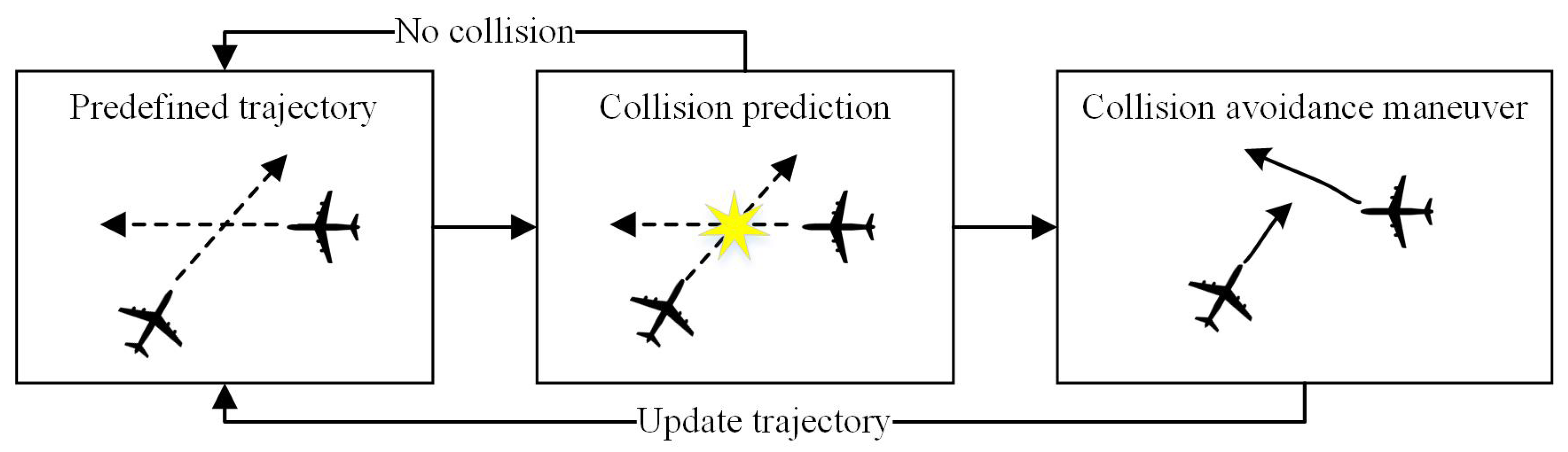
Figure 4.
Representation of 3D state space for a UAV.
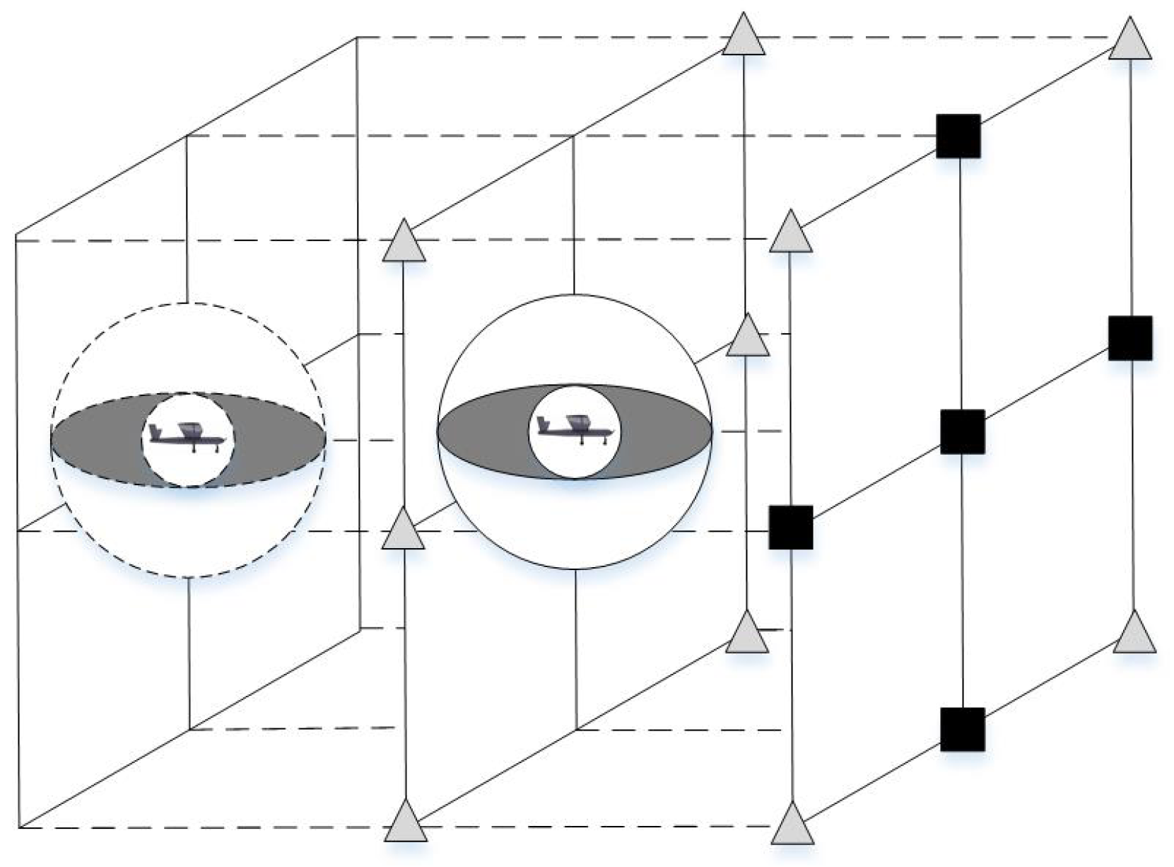
Figure 5.
The process of collision prediction and avoidance maneuver.

Figure 6.
The situation and results in Scenario 1. (a) The initial collision-free trajectory and total distance in Scenario 1; (b) The 5000th collision-free trajectory and total distance in Scenario 1; (c) The distance changes with iteration number increasing in Scenario 1; (d) The relative distance of the best trajectory in Scenario 1.
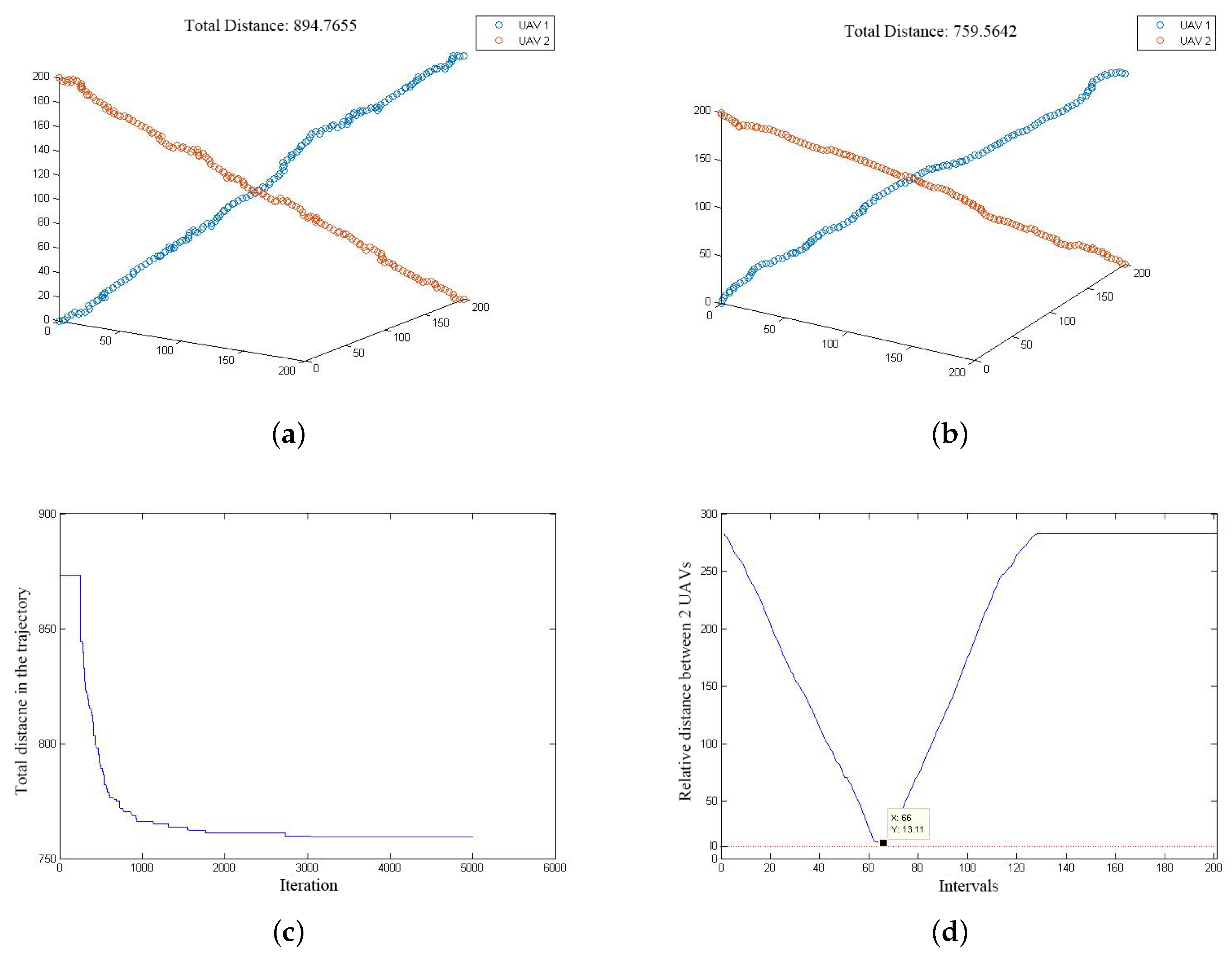
Figure 7.
The situation and results in Scenario 2. (a) The initial collision-free trajectory and total distance in Scenario 2; (b) The 5000th collision-free trajectory and total distance in Scenario 2; (c) The distance changes with iteration number increasing in Scenario 2; (d) The relative distance of the best trajectory in Scenario 2.
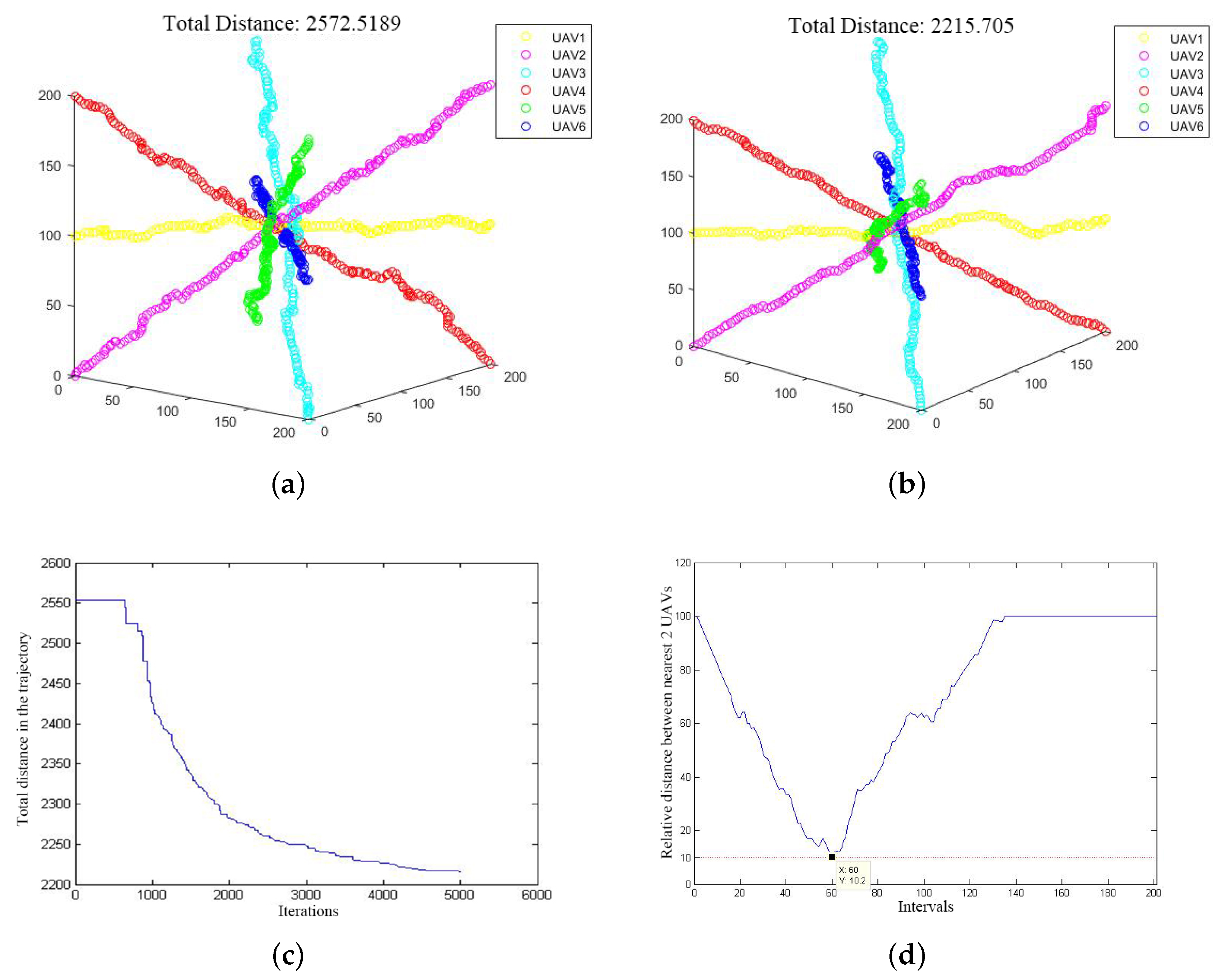
Figure 8.
The potential collision in the real fight of UAVs.


Table 1.
The value of variables in the algorithm for the following scenarios.
| Variables | R | |||||
| Values | 10 | 50 | 100 | 0.5 | 0.2 | 100 |
Table 2.
The initial and destination position of UAVs in Scenario 1.
| UAV Number | Initial Position | Destination Position |
|---|---|---|
| 1 | 0, 0, 0 | 200, 200, 200 |
| 2 | 200, 200, 0 | 0, 0, 200 |
Table 3.
The initial and destination position of UAVs in Scenario 2.
| UAV Number | Initial Position | Destination Position |
|---|---|---|
| 1 | 0, 0, 100 | 200, 200, 100 |
| 2 | 0, 0, 0 | 200, 200, 200 |
| 3 | 200, 0, 0 | 0, 200, 200 |
| 4 | 0, 0, 200 | 200, 200, 0 |
| 5 | 0, 200, 0 | 200, 0, 200 |
| 6 | 200, 0, 100 | 0, 200, 100 |
Table 4.
Run duration of cases with 7 to 20 UAVs in the first 10 iterations.
| The Number of UAVs | Run Duration in 10 Iterations (s) |
|---|---|
| 7 | 35.72 |
| 8 | 62.08 |
| 9 | 72.44 |
| 10 | 84.51 |
| 11 | 98.46 |
| 12 | 90.79 |
| 13 | 123.62 |
| 14 | 148.21 |
| 15 | 223.41 |
| 16 | 265.83 |
| 17 | 293.84 |
| 18 | 295.52 |
| 19 | 304.33 |
| 20 | 387.68 |
Table 5.
Results of evaluation index comprised of other methods. PN: proportional navigation; RRT: rapidly-exploring random tree.
Table 5.
Results of evaluation index comprised of other methods. PN: proportional navigation; RRT: rapidly-exploring random tree.
| Methods | Total Distance of UAVs (m) | Average Velocity (m/s) | Run Duration (s) | Rd |
|---|---|---|---|---|
| PN Method [23] | 20,000 | 176 | 119.66 | 1.0530 |
| RRT Method [27] | 6000 | 40 | 148.70 | 0.9913 |
| ROA1 | 2200 | 2.5 | 2.38 | 0.0027045 |
| ROA5000 | 2200 | 2.5 | 11900 | 13.523 |
© 2017 by the authors. Licensee MDPI, Basel, Switzerland. This article is an open access article distributed under the terms and conditions of the Creative Commons Attribution (CC BY) license (http://creativecommons.org/licenses/by/4.0/).
Share and Cite
MDPI and ACS Style
Yu, T.; Tang, J.; Bai, L.; Lao, S. Collision Avoidance for Cooperative UAVs with Rolling Optimization Algorithm Based on Predictive State Space. Appl. Sci. 2017, 7, 329. https://doi.org/10.3390/app7040329
AMA Style
Yu T, Tang J, Bai L, Lao S. Collision Avoidance for Cooperative UAVs with Rolling Optimization Algorithm Based on Predictive State Space. Applied Sciences. 2017; 7(4):329. https://doi.org/10.3390/app7040329
Chicago/Turabian StyleYu, Tianyuan, Jun Tang, Liang Bai, and Songyang Lao. 2017. "Collision Avoidance for Cooperative UAVs with Rolling Optimization Algorithm Based on Predictive State Space" Applied Sciences 7, no. 4: 329. https://doi.org/10.3390/app7040329
Note that from the first issue of 2016, this journal uses article numbers instead of page numbers. See further details here.