Numerical Control Machine Tool Fault Diagnosis Using Hybrid Stationary Subspace Analysis and Least Squares Support Vector Machine with a Single Sensor

Abstract

Tool fault diagnosis in numerical control (NC) machines plays a significant role in ensuring manufacturing quality. However, current methods of tool fault diagnosis lack accuracy. Therefore, in the present paper, a fault diagnosis method was proposed based on stationary subspace analysis (SSA) and least squares support vector machine (LS-SVM) using only a single sensor. First, SSA was used to extract stationary and non-stationary sources from multi-dimensional signals without the need for independency and without prior information of the source signals, after the dimensionality of the vibration signal observed by a single sensor was expanded by phase space reconstruction technique. Subsequently, 10 dimensionless parameters in the time-frequency domain for non-stationary sources were calculated to generate samples to train the LS-SVM. Finally, the measured vibration signals from tools of an unknown state and their non-stationary sources were separated by SSA to serve as test samples for the trained SVM. The experimental validation demonstrated that the proposed method has better diagnosis accuracy than three previous methods based on LS-SVM alone, Principal component analysis and LS-SVM or on SSA and Linear discriminant analysis.

1. Introduction

Rapid technological development has brought automated and intelligent production processes to manufacturing. Numerical control (NC) machines are flexible, high-performance automated machines that can solve complex and sophisticated processing problems. NC machines play an important role in industries that rely on high precision, high productivity and strong adaptability. However, in practice, owing to tool damage or failure, NC machine processing performance degrades, even leading to scraping of the workpiece. According to our statistics, tool faults account for about 20% of machine failures. Therefore, monitoring and identifying NC machine tool faults in a timely and accurate manner has attracted considerable interest. However, it is a challenge to develop and adopt effective signal processing techniques that can discover the crucial damage information from responsive signals [1].

Owing to the high-speed friction between the tool and the workpiece, the tool is prone to faults such as surface damage or deformation that can lead to a decline in processing quality. The most common resolution is detection of faults by processing and analyzing signals measured by sensors. Traditional signal processing techniques in fault diagnosis include time-domain analysis [2,3] and frequency-domain analysis [4,5].

The main disadvantage of the above two techniques is that only single-domain information is utilized. Although this information may be enough in some simple systems, it is too little for many complex systems. The time–frequency analysis method was proposed to overcome the disadvantages of the above two methods by characterizing the signal in both time and frequency domains. Time–frequency analysis provides a solution to separate physical signals (such as vibrations, acoustic emissions, or cutting forces) in the frequency domain or in the time domain [6,7]. The wavelet analysis method, which can be viewed as an extension of the conventional spectral technique, has been widely used in machinery fault diagnostics, including for rotators, bearings and gears [8,9,10,11]. Wavelet analysis is a local transform of time and frequency. It can effectively extract the information from the signal, and multi-scale analysis can be performed on a signal using expansion and translation operators through a wavelet basis function. However, selection of the wavelet basis function does not yet have unified theoretical criteria [12]. A suitable wavelet basis function can achieve good results, but an improper wavelet basis function could get bad results. The selection of wavelet basis function is subjective and informal in many studies for machine fault diagnosis.

Recently, hybrid intelligent methods have attracted considerable interest for tool fault diagnosis, e.g., Wavelet packet transform (WPT), Artificial neural networks (ANN), and support vector machine (SVM), because they can overcome deficiencies in time-domain or frequency-domain analyses and wavelet transforms. Young-Sun Hong et al. [13] proposed a hybrid tool-wear monitoring method for determining the state of a micro-end mill using wavelet packet transforms and Fisher’s linear discriminant. Xiang et al. [14] developed a personalized machine fault diagnosis method using finite element method, wavelet packet transform and SVM. Guofeng Wang et al. [15] proposed a hybrid-learning-based Gaussian ARTMAP (GAM) network to realize online monitoring of the tool condition. Nagaraj et al. [16] integrated Fisher discriminant ratio and support vector machine (SVM) techniques to classify tool wear states. Amin Jahromi et al. [17] used fuzzy c-means clustering and wavelet analysis to diagnosis tool faults in a high-speed milling process.

These hybrid intelligent methods typically outperform conventional methods; however, they require the signal analyzed to satisfy certain conditions. Such conditions, including a large number of samples for training diagnosis model, independent and identical distribution, white Gaussian noise, or prior information of data, are difficult to meet in practical situation [18,19], especially in time-varying and non-stationary nature of NC machine complex cutting process. 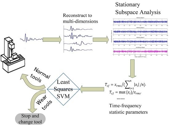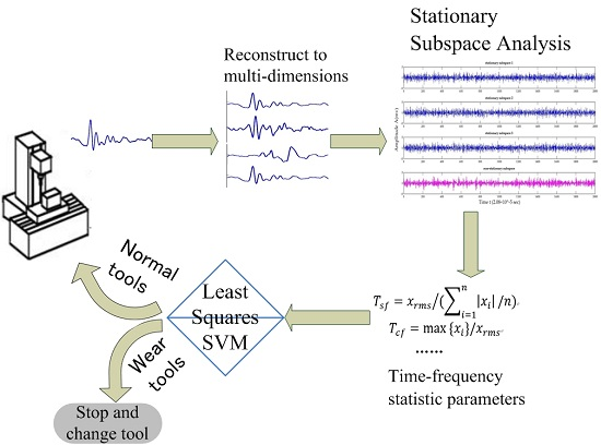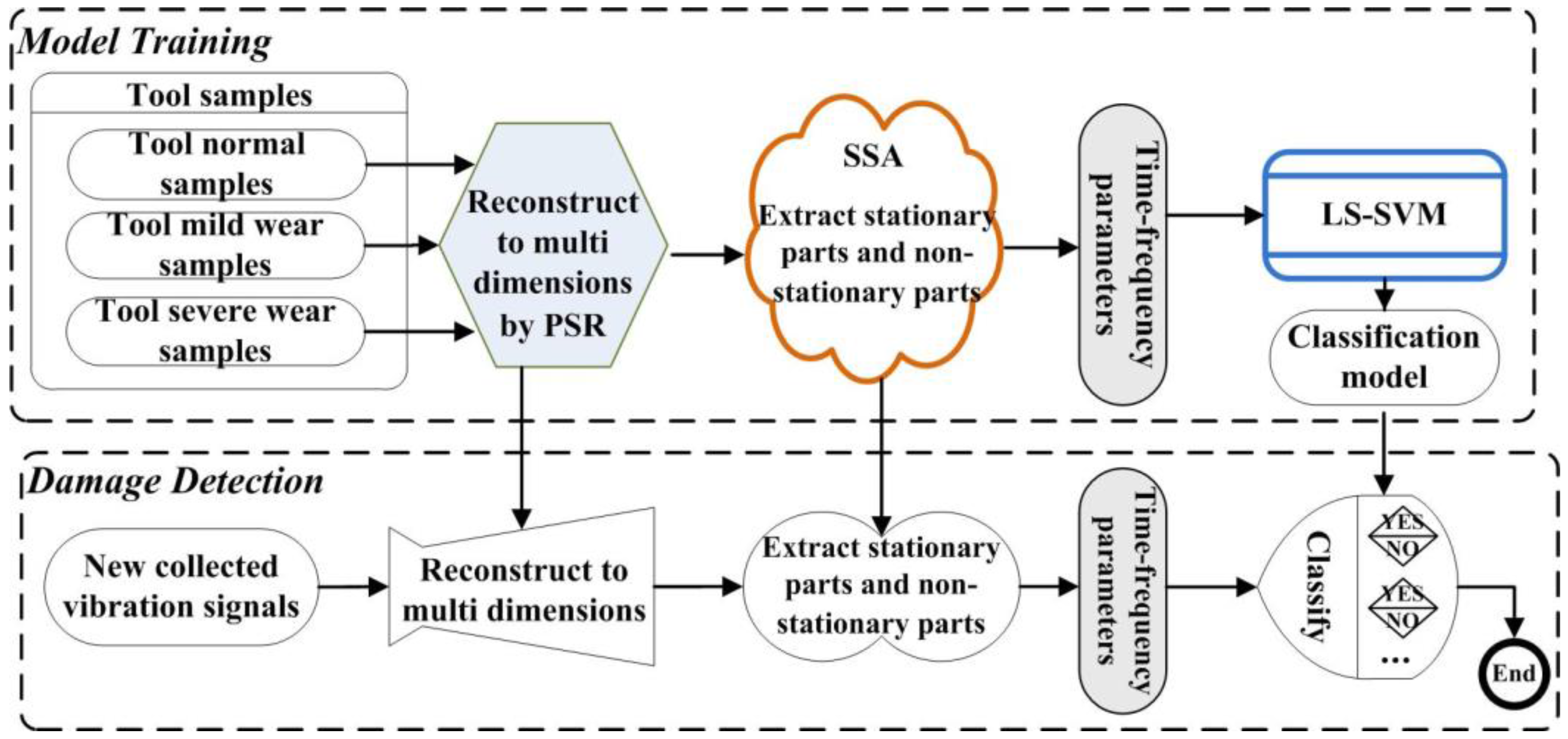Moreover, there is few prior knowledge can be available to detect and diagnose tool faults in NC machine currently [20]. The study of time-varying and non-stationary processes with less prior information is therefore well motivated. In the present paper, a novel fault diagnosis method based on stationary subspace analysis (SSA) and least squares (LS)-SVM is proposed to improve the accuracy of tool fault diagnosis. SSA is a blind source separation algorithm without the need for independency and without prior information of the source signals. It only assumes that the observed signals are a linear superposition of two groups of latent sources (stationary and non-stationary) and the non-stationaries alter the first two moments (mean and covariance matrix) [21]. SSA has been applied successfully to Video Classification [22], electroencephalographic (EEG) [23], Change-point detection [24]. The main goal of this paper is to utilize SSA into tool fault diagnosis of NC Machine, which has been not reported in published researches so far. However, SSA is a multi-dimensional feature exaction method that cannot diagnose tool’ faults directly. LS-SVM and phase space reconstruction technique are introduced in this paper to solve certain requirements of tool fault diagnosis with a single sensor for monitoring cost and processing environment.

The remainder of this paper is organized as follows. Section 2 details the SSA and LS-SVM algorithms. Section 3 provides the architecture of the proposed method. Section 4 describes the experimental design. Section 5 presents the results of the experiment and tests the advantage of the proposed method through a comparative study.

2. Brief Introductions to SSA and LS-SVM

2.1. SSA

Stationary Subspace Analysis (SSA) is a blind source separation algorithm which factorizes a multivariate time series into stationary and non-stationary sources by Paul et al. [21]. In the SSA model, it is assumed that the observed multidimensional time series $X\left(t\right)\in R^D$ is a linear superimposition of two types of sources: stationary sources and non-stationary sources. Its mathematical expression is as follows:

$$X\left(t\right)=AS\left(t\right)=\left(A^s{A}^n\right)\left(\begin{array}{c}{S}^s\left(t\right)\\ S^n\left(t\right)\end{array}\right)$$

(1)

where A is an unknown but time-independent matrix, and is linearly superimposed by coefficient matrix $A^s$ of the stationary sources and coefficient matrix $A^n$ of the non-stationary sources; $S\left(t\right)$ is the underlying intrinsic data of $X\left(t\right)$, and is linearly superimposed by the stationary sources $S^s\left(t\right)\in R^d$ and the non-stationary sources $S^n\left(t\right)\in R^{D-d}$. The aim of the SSA is to estimate the inverse matrix ${\widehat{A}}^{-1}$ separating the stationary sources from non-stationary sources in $X\left(t\right)$. That is, we want to find a demixing matrix, ${\widehat{A}}^{-1}=\left[\begin{array}{c}{B}^s\\ B^n\end{array}\right]$ with $B^s\in R^{d\times D}$ and $B^n\in R^{\left(D-d\right)\times D}$ that consists of the matrixes $B^s$ and $B^n$ for the stationary and non-stationary directions, respectively. Thus, if we apply such an ideal demixing ${\widehat{A}}^{-1}$ to the observed data $X\left(t\right)$,

$$\left[\begin{array}{c}{\widehat{S}}_t^s\\ {\widehat{S}}_t^n\end{array}\right]={\widehat{A}}^{-1}X\left(t\right)={\widehat{A}}^{-1}A\left[\begin{array}{c}{S}_t^s\\ S_t^n\end{array}\right]=\left[\begin{array}{cc}{B}^s{A}^s& B^s{A}^n\\ B^n{A}^s& B^n{A}^n\end{array}\right]\left[\begin{array}{c}{S}_t^s\\ S_t^n\end{array}\right]$$

(2)

The SSA algorithm uses the optimal stationary signal recognition criteria, only the stationary source signal $S_t^s$ and n-space can be uniquely determined, and the non-stationary source signal $S_t^n$ can only get its estimate ${\widehat{S}}_t^n$ by maximizing the non-stationary. Among them, the stationary judgment is based on the weak stationary condition, that is, a time series is stationary if its first two moments are constant over time [25].

SSA needs multi-dimensional observed data that some situations cannot satisfy, owing to working conditions and experimental cost. In NC machine tool fault diagnosis, only one sensor can be used in some situations due to monitoring cost and processing environment, and the observed data are one-dimensional. To use SSA to extract stationary source and non-stationary source signals, the one-dimensional observed data should be expanded into multi-dimensional data. To accomplish this, phase space reconstruction (PSR) is introduced in this paper. PSR is a reconstructing space technology in Chaos theory according to the delay coordinate method [26]. PSR can be used to expand the dimensionality of a system for studying the characteristics of the system without prior knowledge about the structure and parameters of the system. The idea of PSR is that the evolution of any component in a system is determined by its interaction with other components. The time series implies the development process of each component. Considering a single component, PSR takes some measurement processing in fixed time delay point as a new dimension, the value of delay is considered as a new coordinate. By repeating this process at different time points, many of these points generate a new space.

For one-dimensional time series $X\left(t\right)$, different time delays 0, t, 2t, ..., (m − 1)t are used to construct a m-dimensional phase space vector:

$$X_i\left(t\right)=\left\{x\left(t+i\right),x\left(t+i+\tau \right),x\left(t+i+2\tau \right),\dots ,x\left(t+i+\left(m-1\right)\tau \right)\right\},i=0,1,\dots ,m-1$$

where $\tau$ is the time delay and m is the embedding dimension.

$$\mathrm{P}=\left[\begin{array}{cccc}{x}_1& x_2& \dots & \begin{array}{c}{x}_{N-\left(m-1\right)\tau }\end{array}\\ x_{1+\tau }& x_{2+\tau }& \dots & \begin{array}{c}{x}_{N-\left(m-2\right)\tau }\end{array}\\ ⋮& ⋮& ⋮& ⋮\\ \begin{array}{c}{x}_{1+\left(m-1\right)\tau }\end{array}& \begin{array}{c}{x}_{2+\left(m-1\right)\tau }\end{array}& \dots & x_N\end{array}\right]$$

Values of m and $\tau$ can be obtained using the autocorrelation function method and false nearest neighbor method [27,28].

The process of SSA is described as Algorithm 1.

Algorithm 1. Finding non-stationary subspaces by SSA and PSR

Given observed signal $x\left(t\right)$, number of time periods $\mathrm{N}\left(\mathrm{N}\ge \left(\mathrm{D}-\mathrm{d}\right)/2+2\right)$

Step 1: Calculate parameters m and $\tau$ using the autocorrelation function method and false nearest neighbor method. Step 2: Reconstruct $x\left(t\right)$ to multi-dimensional signal $X\left(t\right)$ using PSR. Step 3: Divide $X\left(t\right)$ into $\mathrm{N}$ continuous time periods, and calculate the mean ${\overline{x}}_i$ and covariance ${\hat{\mathsf{\Sigma }}}_i$ of each time period, for an arbitrary choice of $B^s$, get the estimated mean ${\overline{x}}_{s,i}=B^s{\overline{x}}_i$ and covariance matrix ${\hat{\mathsf{\Sigma }}}_{s,i}=B^s{\hat{\mathsf{\Sigma }}}_i$ in each time period. Step 4: Measure the difference between the estimated stationary signal distribution and normal distribution in each time period usingKullback-Leibler (KL) divergence. Sum all period KL divergences, and construct the objective function $\mathrm{L}\left(B^s\right)$ with independent variable $B^s$. Minimizing the objective function $\mathrm{L}\left(B^s\right)$ using gradient descent based algorithm described in [25], obtain the optimal stationary projection ${\widehat{B}}^s$, and estimate the stationary source signal ${\widehat{S}}_t^s\mathrm{L}\left({\widehat{B}}^s\right)=\min \mathrm{L}\left(B^s\right)=\min {\displaystyle \sum }_{i=1}^n{D}_{KL}\left[Norm\left({\overline{x}}_{s,i},{\hat{\mathsf{\Sigma }}}_{s,i}\right)||Norm\left(0,\mathrm{I}\right)\right]$ according to Equation (2). Step 5: Construct the objective function $\mathrm{G}\left(B^n\right)$ with steps (1) and (2) above. Maximizing the objective function $\mathrm{G}\left(B^n\right)$ using the optimization algorithm in Step 4, obtain the optimal non-stationary projection ${\widehat{B}}^n$, and according to Equation (2) estimate the non-stationary source signal ${\widehat{S}}_t^n\mathrm{G}\left({\widehat{B}}^n\right)=\max \mathrm{G}\left(B^n\right)=\max {\displaystyle \sum }_{i=1}^n{D}_{KL}\left[Norm\left({\overline{x}}_{n,i},{\hat{\mathsf{\Sigma }}}_{n,i}\right)||Norm\left(0,\mathrm{I}\right)\right]$.

2.2. Least Squares SVM

The support vector machine (SVM) is a powerful nonlinear classification method for overcoming the drawback of traditional linear classification methods. SVM is a kernel-based method. It maps the low-dimension nonlinear structures of signals to a high-dimensional (possibly infinite) linear feature space using the kernel trick. Least squares (LS)-SVM [29], as with the artificial neural network method, does not need training with large data sets to estimate corresponding parameters; it is numerically inexpensive and less overfitting in the training process [30].

Given a training data set $\left\{\left(x\left(t\right),y\left(t\right)\right),t=1,2,\dots ,N\right\}$, $x\left(t\right)\in R^m$ is the input data, $y\left(t\right)\in R$ is the output corresponding to $x\left(t\right)$, and N is the training samples number. In LS-SVM, The estimation model is $y_t=w^T\phi \left(x_t\right)+b+e_t$, where $\phi \left(\right)$ is a nonlinear transformation that maps $x\left(t\right)$ to the high-dimensional feature space, w is weight vector, b is intercept, and $e_t$ is the error term that is assumed to be independent and identically distributed with zero mean and finite variance [31]. The unknowns w and b can be determined from a convex optimization problem as follows:

$$\min J\left(w,e\right)=\frac{1}{2}(w^{T}w+c{\displaystyle \sum }_{t=1}^N{e}_t^2)$$

(3)

Such that $y_t=w^T\phi \left(x_t\right)+b+e_t$, $t=1,2,\dots ,N$.

According to [29,30], the LS-SVM model can be expressed in dual form as $\widehat{y}\left(z\right)={{\displaystyle \sum }}_{t=1}^N{\alpha }_{t}K\left(z,x_t\right)+b$. Note that the unknown items w and $\phi \left(\right)$ are not included in the dual model; the mapping transformation operations are achieved implicitly through the use of kernel function $K(,)$. That is, it is necessary to find the expression of mapping function $\phi \left(\right)$. For the kernel function $K(,)$, a function satisfying the Mercer theorem can be used. There are several choices presently, including the linear kernel, the perceptron kernel, the spline kernel, or the RBF (Radial Basis Function) kernel.

In the LS-SVM model, it is required to optimize the parameter c in Equation (3) and the kernel parameter according to the kernel function selected, e.g., $\sigma$ in Gaussian RBF kernel ($K\left(x_p,x_q\right)=\exp (-\frac{{\Vert x_p-x_q\Vert }^2}{2{\sigma }^2})$). A fast leave-one-out cross validation optimization [32] can be used for optimizing these parameters.

However, LS-SVM cannot deal with time series directly. To generate the fault features training samples, some time- and frequency-domain indexes are selected from the non-stationary signals by SSA, and are taken as inputs to train the LS-SVM classifier model. In this paper, 10 dimensionless statistical indexes in time and frequency domains are chosen [33,34]. A brief mathematical description of these indexes is summarized in

Table 1. Ten time domain and frequency domain dimensionless statistical parameters ¹.

Domain	Indexes	Formula
Time	Shape factor Tsf	$T_{sf}=x_{rms}/\left({{\displaystyle \sum }}_{i=1}^n\left|x_i\right|/n\right)$
	Crest factor Tcf	$T_{cf}=\max \left\{x_i\right\}/x_{rms}$
	Kurtosis Tk	$T_{ku}=\frac{{{\displaystyle \sum }}_{i=1}^n{\left(x_i-\overline{x}\right)}^4}{n{S}^4}-3$
	Skewness Tsk	$T_{sk}=\frac{{{\displaystyle \sum }}_{i=1}^n{\left(x_i-\overline{x}\right)}^3}{n{S}^3}$
	Kurtosis factor Tkf	$T_{kf}=T_k/x_{rms}$
Frequency	Stabilization ratio Fsr	$F_{sr}=({{\displaystyle \sum }}_{i=1}^{\frac{n}{2}}{f}_i^2{P}_i)/\sqrt{{{\displaystyle \sum }}_{i=1}^{n/2}\left(f_i^4{P}_i\right){{\displaystyle \sum }}_{i=1}^{n/2}{P}_i}$
	Wave-height ratio Fwr	$F_{wr}=\max \left\{P_i\right\}/\sqrt{\frac{2}{n}{{\displaystyle \sum }}_{i=1}^{n/2}{P}_i^2}$
	Average Frequency Faf	$F_{af}=\sqrt{{{\displaystyle \sum }}_{i=1}^{n/2}\left(f_i{P}_i\right)}/\sqrt{{{\displaystyle \sum }}_{i=1}^{n/2}{P}_i}$
	Frequency high-low ratio Ffhr	$F_{fhr}=\left({{\displaystyle \sum }}_{i=\frac{n}{4}}^{\frac{n}{2}}{P}_i\right)/\left({{\displaystyle \sum }}_{i=1}^{\frac{n}{4}}{P}_i\right)$
	Modified equivalent bandwidth Fmeb	$F_{meb}=\sqrt{{{\displaystyle \sum }}_{i=1}^{n/2}\left({\left(f_i-\overline{f}\right)}^2{P}_i\right)}/\sqrt{{{\displaystyle \sum }}_{i=1}^{n/2}{P}_i}$

¹ x_i is a signal series for i = 1, 2, …, n, n is the number of data points, $\overline{x}$ and S are the mean and the standard deviation of x_i, $x_{rms}=\sqrt{{{\displaystyle \sum }}_{i=1}^n{x}_i^2/n}$; f_i is the frequency signal with x_i by FFT, P_i is the power spectrum of f_i, $\overline{f}=\sqrt{{{\displaystyle \sum }}_{i=1}^n{f}_i/n}$.

.

The process of LS-SVM classifier according to [32] is described as Algorithm 2.

Algorithm 2. Training LS-SVM classifier by leave-one-out cross validation

Given data $\left(N{T}_i,Y_i\right),i=1,\dots , n$, $N{T}_i$ is the feature indexes of the i-th signal and $Y_i$ is the class corresponding to the i-th sample.

Step 1: Calculate 10 dimensionless time–frequency indexes of each $N{T}_i$, as inputs of LS-SVM for classification. Step 2: Standardize the input data, and select a kernel function. Find the optimal parameter c by solving the optimization problem (3). Step 3: Set candidate tuning sets for kernel parameter, perform fast leave-one-out test for each candidate with the optimal parameter c obtained in Step 2, and take the result that obtains the highest test accuracy as the optimal kernel parameter. Step 4: With the optimal kernel parameter obtained in Step 3, go back to Step 2 to refine parameter c.

3. Damage Diagnosis Approach Based on Hybrid SSA and LS-SVM

The damage diagnosis approach for NC machine tools proposed in this paper includes two phases. The first phase focuses on model training and obtains sample feature parameters for different tool states. First, reconstructed multi-dimensional signals are transformed by PSR and the stationary and non-stationary parts are extracted using SSA. Subsequently, some dimensionless time–frequency parameters in the non-stationary component are calculated, to be used as sample data for LS-SVM classification. The second phase is damage detection for tools whose state is unknown. The specific procedure is constructed through the main steps shown in Figure 1.

The process of the proposed SSA + LS-SVM method is described as Algorithm 3.

Algorithm 3. Damage diagnosis approach based on SSA + LS-SVM

Step 1: Model training Measure vibration time signals of NC machine in three damage classes (normal, mild wear and severe wear) n times each. For each signal, find the stationary and non-stationary sources using Algorithm 1. Train the LS-SVM classifier model using Algorithm 2 and the Gaussian RBF kernel function.

Step 2: Damage detection Periodically collect vibration time-domain signals from the NC machine under operating condition while the state of the tool is unknown and to identify its class. Find the unknown tool’s stationary and non-stationary signal sources using Algorithm 1, using the reconstructed parameters from Step 1. Calculate 10 dimensionless time–frequency indexes for the non-stationary signal source and identify the class of the unknown signal using the trained LS-SVM classifier.

4. Experimental Design

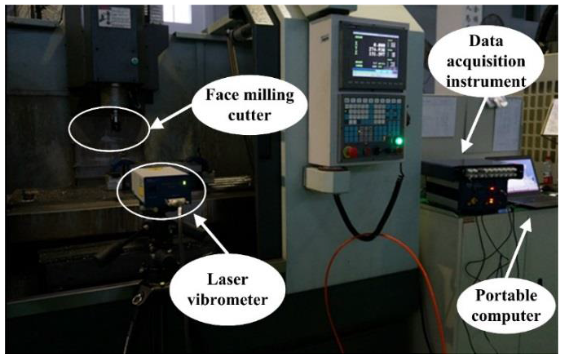
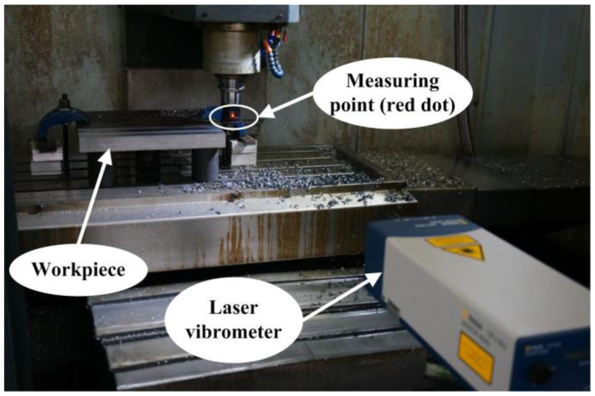
The experimental setup for tool fault detection under operating conditions is illustrated in Figure 2. The GSVM714A NC milling machine (Deusi Numerical Control Technologies Co., Ltd., Nanjing, China) is used for the experimental test. The tools used in this test are carbide cutting tools (#RPMW1003#) and a face milling cutter with four teeth (#EMR 5R160-40-8T#). Owing to their effectiveness and convenience [35,36], vibration signals were collected indirectly in operation states using a laser vibrometer from Polytec Inc. (shown in Figure 3). These vibration signals were sent to a data acquisition instrument (MI-7016 Avant, Econ Technologies Co., Ltd., Hangzhou, China) and stored on a personal computer.

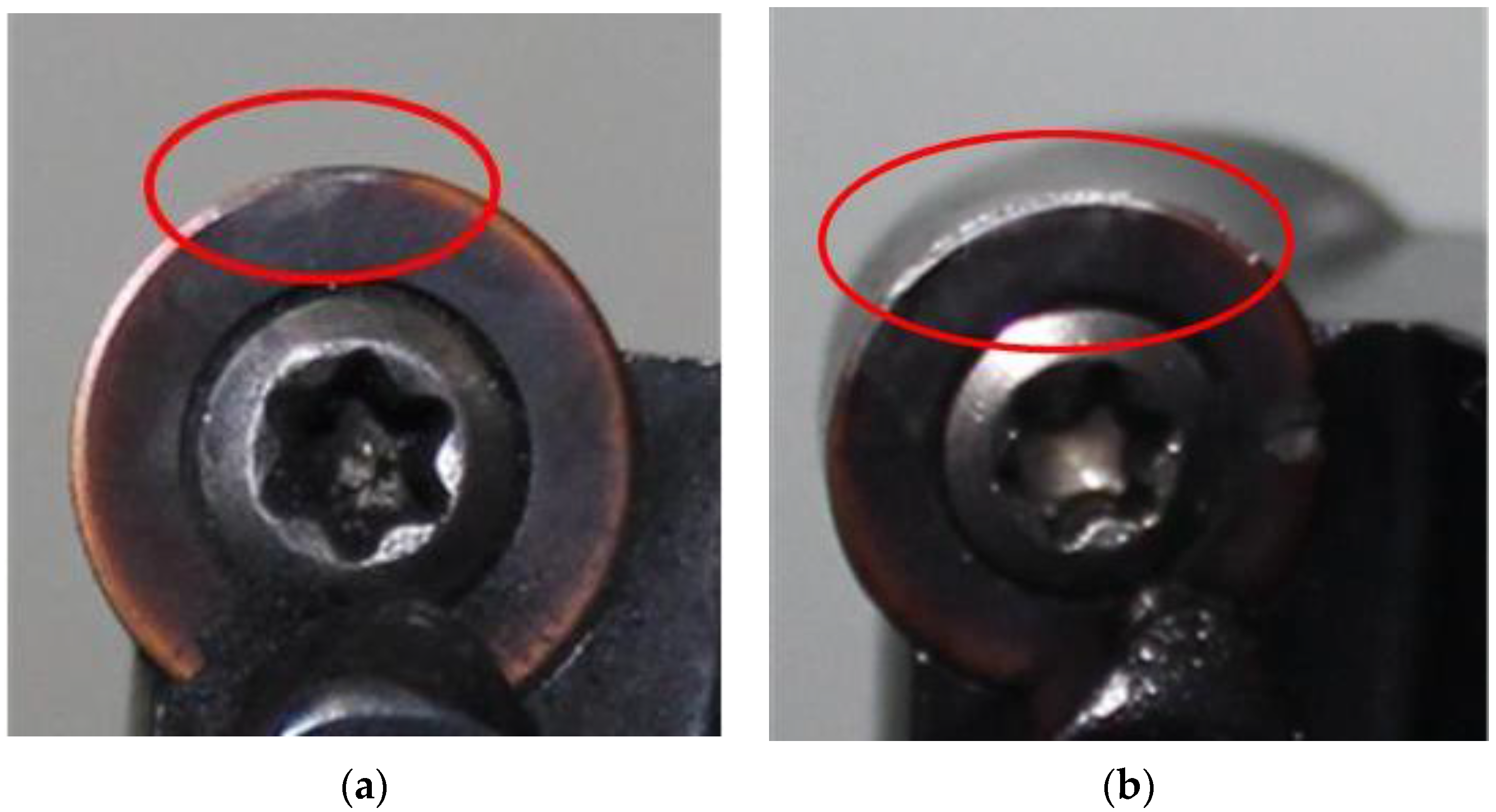
Tools in this experiment are considered to be in one of three states: (1) normal; (2) mild wear; or (3) severe wear (as shown in Figure 4). Aluminum alloy samples #7075-T351# (150 mm × 100 mm × 500 mm) were fixed on the machining center. Cutting speed was set to 1000 rpm and cutting depth to 1 mm.

It was assumed that all investigated tools have the same damage mechanism. Vibration signals in three tool fault classes are measured and total 180 samples were taken, out of which 60 samples from each condition of the tool for a time interval of 1s at sampling frequency of 48 kHz. 60 samples of each tool condition divided into two parts: 40 samples as training set and 20 samples as testing set. The training set is used to train the LS-SVM model in MATLAB 2012R.

5. Result and Discussion

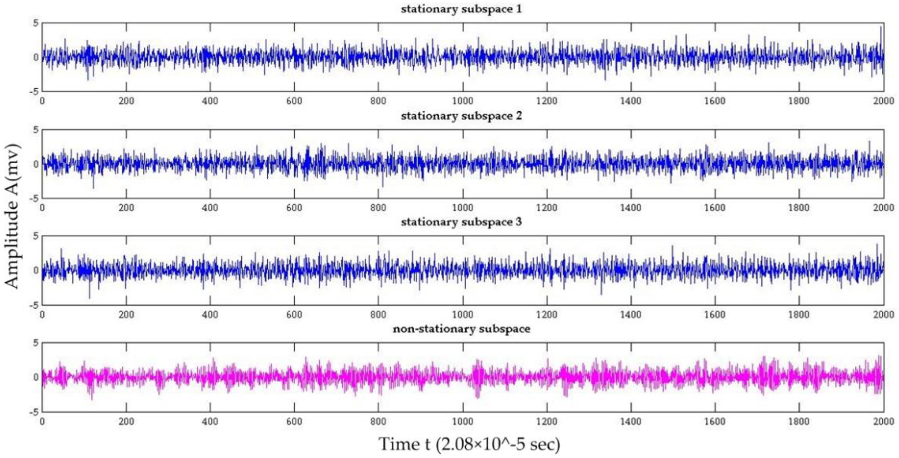
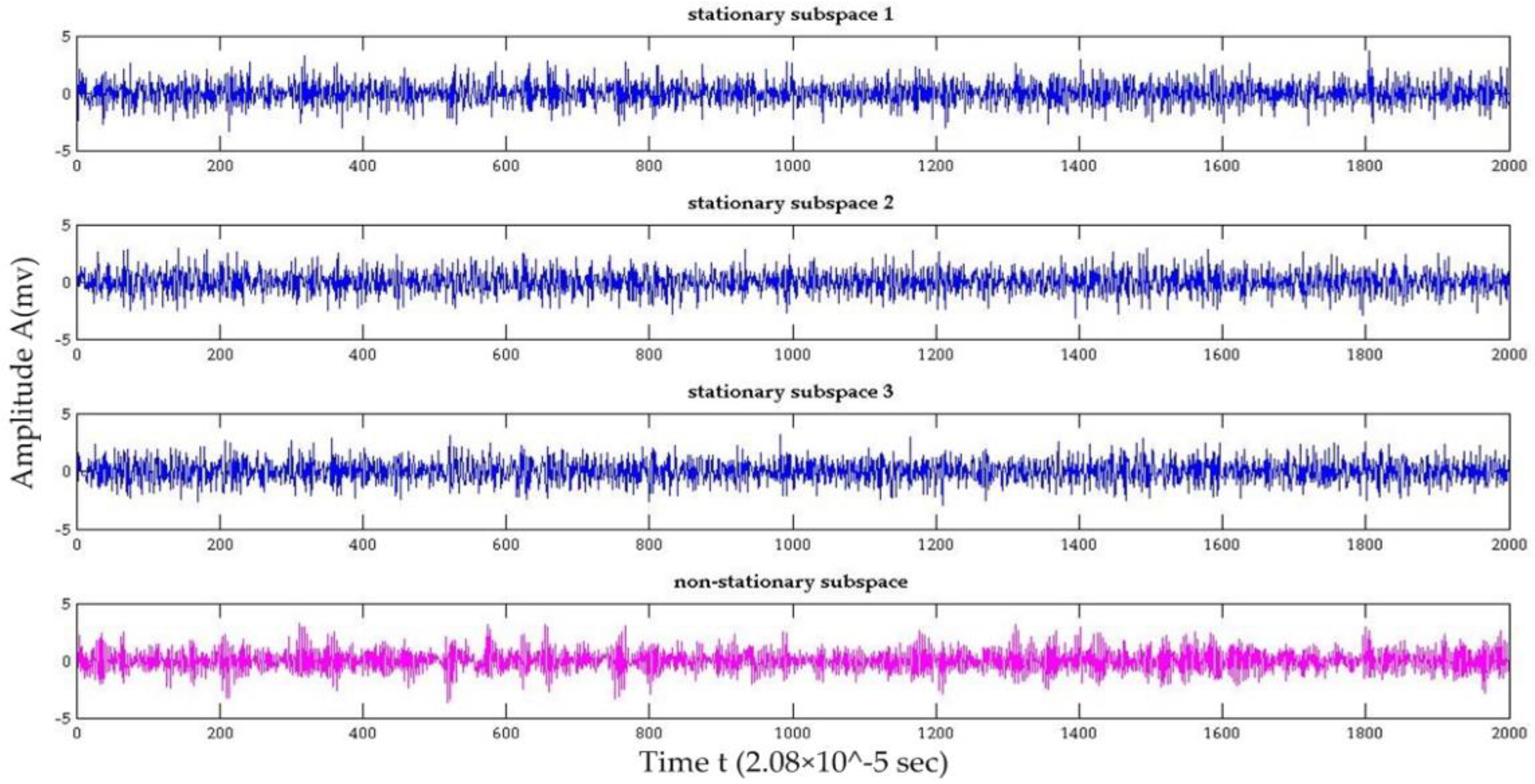
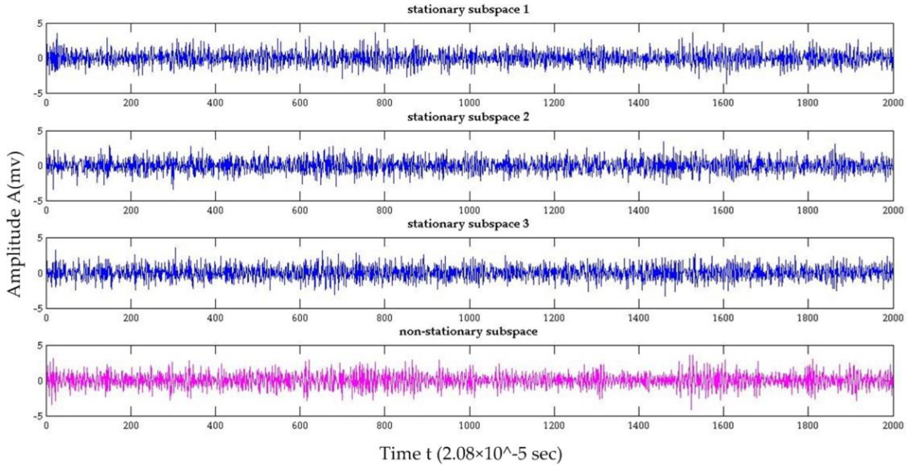
In the first phase model training, values for time delay ($\tau$ = 10) and embedding dimension (m = 4) are obtained using the autocorrelation function method and false nearest neighbor method [27,28]. These are chosen as inputs for the SSA decomposition, and one non-stationary source and three stationary sources signals are extracted. There are two reasons for setting one non-stationary source signal: (1) non-stationary source contains more fault feature information to distinguish different fault classes than stationary source; (2) one source signal is convenient to calculate time- and frequency-domain indexes for follow-up process in the proposed approach. SSA training data for three damage classes are shown in Figure 5, Figure 6 and Figure 7. Ten dimensionless time–frequency parameters were chosen from the non-stationary source of each class, and these were used as the input data for LS-SVM. The Gaussian RBF kernel ($K\left(x_p,x_q\right)=\exp (-\frac{{\Vert x_p-x_q\Vert }^2}{2{\sigma }^2})$) was selected, and the kernel parameter $\sigma$ is optimized usinga fast leave-one-out cross validation optimization proposed in [32].

The classification results of the proposed SSA + LS-SVM method are shown in

Table 2. Result of stationary subspace analysis (SSA) + least squares support vector machine (LS-SVM), original LS-SVM, Principal Component Analysis (PCA) + LS-SVM and SSA + linear discriminant analysis (LDA) with training set.

Methods	Training Classes	Training Result			Classification Accuracy
		Normal Tool	Mild Wear Tool	Severe Wear Tool
SSA + LS-SVM proposed	normal tool	40	0	0	100%
	mild wear tool	0	35	5	87.5%
	severe wear tool	0	3	37	92.5%
Original LS-SVM	normal tool	37	3	0	92.5%
	mild wear tool	4	29	7	72.5%
	severe wear tool	0	8	32	80%
PCA + LS-SVM	normal tool	38	2	0	95%
	mild wear tool	5	30	5	75%
	severe wear tool	2	6	32	80%
SSA + LDA	normal tool	31	9	0	77.5%
	mild wear tool	6	26	8	65%
	severe wear tool	0	11	29	72.5%

and

Table 3. Result of SSA + LS-SVM, original LS-SVM, PCA + LS-SVM and SSA + LDA with testing sets.

Methods	Testing Classes	Testing Result			Classification Accuracy
		Normal Tool	Mild Wear Tool	Severe Wear Tool
SSA + LS-SVM proposed	normal tool	20	0	0	100%
	mild wear tool	0	16	4	80%
	severe wear tool	0	3	17	85%
Original LS-SVM	normal tool	18	2	0	90%
	mild wear tool	4	13	3	65%
	severe wear tool	0	5	15	75%
PCA + LS-SVM	normal tool	19	1	0	95%
	mild wear tool	5	e	1	70%
	severe wear tool	1	4	15	75%
SSA + LDA	normal tool	14	6	0	70%
	mild wear tool	7	10	3	50%
	severe wear tool	2	5	13	65%

. Table 2 presents the classification results with training set, all normal tools can be correctly identified; however, the accuracy of the mild wear and severe wear tools is 87.5% and 92.5%, respectively. Five mild wear tools were identified wrongly as severe wear tools, and three severe wear tool were identified as mild wear tools. Table 3 shows the classification results with testing set, all normal tools can be correctly identified; however, the accuracy of the mild wear and severe wear tools is 80% and 85%, respectively. Four mild wear tools were identified as severe wear tools, and three severe wear tool were identified as mild wear tools. Fortunately, as shown in Table 2 and Table 3, the proposed method can significantly distinguish between normal tools and wear tools (included mild and severe wears) both in training sets and testing sets.

The proposed SSA + LS-SVM method was compared with the original LS-SVM, PCA (Principal Component Analysis) + LS-SVM, and with SSA + LDA (linear discriminant analysis). The original LS-SVM method means that the original vibration signals measured in experiment are the input of LS-SVM, in which do not extract signals by SSA and PSR. Its algorithm calculates 10 dimensionless time–frequency indexes (described in Table 1) from the original vibration signals and be used as inputs for training the LS-SVM classifier model. The PCA + LS-SVM method substitute SSA for PCA in Algorithm 3, that is to say, PCA is used to feature extraction. PCA is a popular and powerful blind source separation algorithm. It constructs a low-dimensional representation of the data that describes the variance in the data as much as possible. It is achieved by finding a linear basis of reduced dimensionality for the data, in which the amount of variance in the data is maximal [37]. To implement the PCA + LS-SVM method, 10 dimensionless time–frequency indexes (described in Table 1) of each signal are calculated as the input of PCA, and 10 principal components transformed by PCA are selected as the input of LS-SVM. The SSA + LDA method substitute LS-SVM for LDA in Algorithm 3, that is to say, LDA is used as the classifier model. LDA is a linear classifier that uses a generalization of Fisher’s linear discriminant; its aim is to find a linear combination of features that characterizes classes of objects or events [38].

As shown in Table 2 and Table 3, the original LS-SVM, PCA + LS-SVM and SSA + LDA methods are less accurate than the proposed SSA + LS-SVM method. In the original LS-SVM method, the accuracy of the normal, mild wear and severe wear groups with training sets was about 80%, and even low to 65% with testing sets, 22 tools in training sets and 14 tools in testing sets were erroneously categorized. In the PCA + LS-SVM method, the accuracy of the normal, mild wear and severe wear groups with training sets were higher than original LS-SVM method, 20 tools in training sets and twelve tools in testing sets were erroneously categorized. However, with the tool failure gradually becoming serious, its advantage is reduced over original LS-SVM method. In the SSA + LDA method, the accuracy of mild wear group with training sets and testing sets was 65% and 50%, 34 tools in training sets and 23 tools in testing sets were erroneously categorized. The three methods could not discriminate between normal tools and wear tools effectively. The proposed SSA + LS-SVM method in this paper outperformed the original LS-SVM, PCA + LS-SVM and SSA + LDA methods.

6. Conclusions

The present study proposes a damage diagnosis approach to NC machine tools based on SSA and LS-SVM. First, the original data are transformed from one-dimensional data into high-dimensional signals using PSR. The SSA method is applied to extract stationary and non-stationary parts from multi-dimensional signals without the need for independency and without prior information of the source signals. Subsequently, the selected non-stationary components were analyzed for classification using LS-SVM. Ten dimensionless parameters in the time-frequency domain were extracted and used as inputs for LS-SVM. The proposed SSA + LS-SVM method was applied to NC milling machine tools. The results show that the proposed SSA + LS-SVM method outperforms the original LS-SVM, PCA + LS-SVM and SSA + LDA methods. The achieved accuracy of the proposed SSA + LS-SVM method was higher than 80%, whereas that of the original LS-SVM, PCA + LS-SVM and SSA + LDA was as low as 65%, 70% and 50%, respectively. Moreover, the proposed method can significantly distinguish between normal tools and wear tools, which cannot be realized through the other three methods. Furthermore, it is possible to apply the proposed method to other fault diagnosis areas, e.g., electric motors, in which the signals of bars of an induction motor are time varying, and non-stationary [39,40].

However, classification accuracy of the proposed SSA + LS-SVM method for mild wear and severe wear with testing sets is just 80% and 85%, respectively. Future work will focus on improvement of this accuracy. The stationary sources extracted by SSA will be utilized in future studies to improve the accuracy in identifying mild wear tools.

References

1. Lei, Y.; Lin, J.; He, Z.; Zuo, M.J. A review on empirical mode decomposition in fault diagnosis of rotating machinery. Mech. Syst. Signal Proc. 2013, 35, 108–126. [Google Scholar] [CrossRef]
2. Amer, W.; Grosvenor, R.I.; Prickett, P.W. Sweeping filters and tooth rotation energy estimation (TREE) techniques for machine tool condition monitoring. Int. J. Mach. Tools Manuf. 2006, 46, 1045–1052. [Google Scholar] [CrossRef]
3. Lv, J.; Wang, J.; Wang, M.; Wu, Y. Research on tool wear condition monitoring Based on combination of SOM and HMM. China Mech. Eng. 2010, 21, 1531–1535. [Google Scholar]
4. Shen, Z.; He, N.; Li, L. Monitoring of Tool Wear in Hard Milling. China Mech. Eng. 2009, 20, 1582–1586. [Google Scholar]
5. Zaghbani, I.; Lamraoui, M.; Songmene, V.; Thomas, M.; ElBadaoui, M. Robotic high speed machining of aluminum alloys. Adv. Mater. Res. 2011, 188, 584–589. [Google Scholar] [CrossRef]
6. RodolfoHaber, E.; JoseJimenez, E.; RoneiPeres, C.; JoseAlique, R. An investigation of tool-wear monitoring in a high-speed machining process. Sens. Actuators A Phys. 2004, 116, 539–545. [Google Scholar]
7. Jachan, M.; Matz, G.; Hlawatsch, F. Time-frequency ARMA models and parameter estimators for under spread non stationary random processes. IEEE Trans. Signal Process. 2007, 55, 4366–4381. [Google Scholar] [CrossRef]
8. Kankar, P.K.; Sharma, S.C.; Harsha, S.P. Rolling element bearing fault diagnosis using autocorrelation and continuous wavelet transform. J. Vib. Control. 2011, 17, 2081–2094. [Google Scholar] [CrossRef]
9. Guo, X.; Shen, C.; Chen, L. Deep Fault Recognizer: An Integrated Model to Denoise and Extract Features for Fault Diagnosis in Rotating Machinery. Appl. Sci. 2017, 7, 41. [Google Scholar] [CrossRef]
10. Singh, M.; Kumar, R. Thrust bearing groove race defect measurement by wavelet decomposition of pre-processed vibration signal. Measurement 2013, 46, 3508–3515. [Google Scholar] [CrossRef]
11. Jena, D.P.; Panigrahi, S.N.; Kumar, R. Gear fault identification and localization using analytic wavelet transform of vibration signal. Measurement 2013, 46, 1115–1124. [Google Scholar] [CrossRef]
12. Feng, Z.; Liang, M.; Chu, F. Recent advances in time-frequency analysis methods for machinery fault diagnosis: A review with application examples. Mech. Syst. Signal Process. 2013, 38, 165–205. [Google Scholar] [CrossRef]
13. Hong, Y.-S.; Yoon, H.-S.; Moon, J.-S.; Cho, Y.-M.; Ahn, S.-H. Tool wear monitoring during micro-end milling using wavelet packet transform and Fisher’s linear discriminant. Int. J. Precis. Eng. Manuf. 2016, 17, 845–855. [Google Scholar] [CrossRef]
14. Xiang, J.; Zhong, Y. A Novel Personalized Diagnosis Methodology Using Numerical Simulation and an Intelligent Method to Detect Faults in a Shaft. Appl. Sci. 2016, 6, 414. [Google Scholar] [CrossRef]
15. Wang, G.; Yang, Y.; Guo, Z. Hybrid learning based Gaussian ARTMAP network for tool condition monitoring using selected force harmonic features. Sens. Actuators A 2013, 203, 394–404. [Google Scholar] [CrossRef]
16. Bhat, N.N.; Dutta, S.; Vashisth, T.; Pal, S.; Pal, S.K.; Sen, R. Tool condition monitoring by SVM classification of machined surface images in turning. Int. J. Adv. Manuf. Technol. 2016, 83, 1487–1502. [Google Scholar] [CrossRef]
17. Torabi, A.J.; Er, M.J.; Li, X.; Lim, B.S.; Peen, G.O. Application of Clustering Methods for Online Tool Condition Monitoring and Fault Diagnosis in High-Speed Milling Processes. IEEE Syst. J. 2016, 10, 721–732. [Google Scholar] [CrossRef]
18. Zhu, K.; Wong, Y.S.; Hong, G.S. Wavelet analysis of sensor signals for tool condition monitoring- A review and some new results. Int. J. Mach. Tools Manuf. 2009, 49, 537–553. [Google Scholar] [CrossRef]
19. Torabi, A.J.; Meng, J.E.; Li, X.; Lim, B.S. A Survey on Artificial Intelligence-Based Modeling Techniques for High Speed Milling Processes. IEEE Syst. J. 2014, 9, 1069–1080. [Google Scholar] [CrossRef]
20. Lamraoui, M.; Thomas, M.; Badaoui, M.E. Cyclostationarity approach for monitoring chatter and tool wear in high speed milling. Mech. Syst. Signal Process. 2014, 44, 177–198. [Google Scholar] [CrossRef]
21. Von Bünau, P.; Meinecke, F.C.; Király, F.C. Finding stationary subspaces in multivariate time series. Phys. Rev. Lett. 2009, 103, 1–4. [Google Scholar] [CrossRef] [PubMed]
22. Baktashmotlagh, M.; Harandi, M.; Lovell, B.C.; Salzmann, M. Discriminative non-linear stationary subspace analysis for video classification. IEEE Trans. Pattern Anal. Mach. Intell. 2014, 36, 2353–2366. [Google Scholar] [CrossRef] [PubMed]
23. Zeng, H.; Song, A.; Yan, R.; Qin, H. Eog artifact correction from eeg recording using stationary subspace analysis and empirical mode decomposition. Sensors 2012, 13, 14839–14859. [Google Scholar] [CrossRef] [PubMed]
24. Blythe, D.A.; von Bünau, P.; Meinecke, F.C.; Müller, K.R. Feature Extraction for Change-Point Detection using stationary subspace analysis. IEEE Trans. Neural Netw. Learn. Syst. 2012, 23, 631–643. [Google Scholar] [CrossRef] [PubMed]
25. Von Bünau, P. Stationary Subspace Analysis: Towards Understanding Non-Stationary Data. Ph.D. Thesis, Berlin Institute of Technology, Berlin, Germany, 2012. [Google Scholar]
26. Packard, N.H.; Crutchfield, J.P.; Farmer, J.D. Geometry from a time series. Phys. Rev. Lett. 1980, 45, 712–716. [Google Scholar] [CrossRef]
27. Kennel, M.; Brown, R.; Abarbanel, H. Determining embedding dimension for phase-space reconstruction using a geometrical construction. Phys. Rev. A 1992, 45, 3403–3411. [Google Scholar] [CrossRef] [PubMed]
28. Chen, K.; Han, B. A Survey of State Space Reconstruction of Chaotic Time Series Analysis. Comput. Sci. 2005, 32, 67–70. [Google Scholar]
29. Suykens, J.A.K. Least squares support vector machines for classification and nonlinear modeling. Neural Netw. World 2000, 10, 29–48. [Google Scholar]
30. Feng, Y.; Jia, B.; Yan, G.; Jia, X. Prediction model of high-speed oblique cutting temperature based on LS-SVM. Int. J. Adv. Manuf. Technol. 2016, 85, 1–8. [Google Scholar]
31. Falck, T.; Dreesen, P.; de Brabanter, K.; Pelckmans, K.; de Moor, B.; Suykens, J.A.K. Least-Squares Support Vector Machines for the identification of Wiener–Hammerstein systems. Control Eng. Pract. 2012, 20, 1165–1174. [Google Scholar] [CrossRef]
32. Ying, Z.; Keong, K.C. Fast Leave-One-Out Evaluation and Improvement on Inference for LS-SVM’s. Proc. ICPR 2004, 1–4. [Google Scholar] [CrossRef]
33. Van Gestal, T.; Suykens, J.A.K.; Lanckriet, G.; Lambrechts, A.; de Moor, B.; Vandewalle, J. Bayesian framework for least squares support vector machine classifiers, gaussian processes and kernel fisher discriminant analysis. Neural Comput. 2002, 14, 1115–1147. [Google Scholar] [CrossRef] [PubMed]
34. Ciabattoni, L.; Cimini, G.; Ferracuti, F.; Grisostomi, M.; Ippoliti, G.; Pirro, M. Bayes error based feature selection: An electric motors fault detection case study. IECON 2015, 003893–003898. [Google Scholar] [CrossRef]
35. Zhou, Y.; Liu, X.; Li, F.; Sun, B.; Xue, W. An online damage identification approach for numerical control machine tools based on data fusion using vibration signals. J. Vib. Control 2015, 21, 2925–2936. [Google Scholar]
36. Xie, H.; Huang, M. Research of numerical control machine tools wear monitoring method based on vibration testing. Instrum. Tech. Sens. 2013, 2, 73–75. [Google Scholar]
37. Van der Maaten, L.J.P.; Postma, E.O.; van den Herik, H.J. Dimensionality reduction: A comparative review. J. Mach. Learn. Res. 2009, 10, 1–41. [Google Scholar]
38. Zhang, X.; Jia, Y. A linear discriminant analysis framework based on random subspace for face recognition. Pattern Recognit. 2007, 40, 2585–2591. [Google Scholar] [CrossRef]
39. Sahraoui, M.; Cardoso, A.J.M.; Ghoggal, A. The Use of a Modified Prony Method to Track the Broken Rotor Bar Characteristic Frequencies and Amplitudes in Three-Phase Induction Motors. IEEE Trans. Ind. Appl. 2015, 51, 2136–2147. [Google Scholar] [CrossRef]
40. Ferracuti, F.; Giantomassi, A.; Iarlori, S.; Ippoliti, G.; Longhi, S. Electric motor defects diagnosis based on kernel density estimation and kullback–leibler divergence in quality control scenario. Eng. Appl. Artif. Intell. 2015, 44, 25–32. [Google Scholar] [CrossRef]
Figure 1. Damage diagnosis procedure based on hybrid Stationary subspace analysis, SSA: stationary subspace analysis, LS-SVM: least squares support vector machine.
Applsci 07 00346 g001
Figure 2. Experiment design.
Applsci 07 00346 g002
Figure 3. Measuring vibration signal by a laser vibrometer.
Applsci 07 00346 g003
Figure 4. Samples of different tool states, (a) mild wear tool; (b) severe wear tool.
Applsci 07 00346 g004
Figure 5. SSA results of normal tool sample.
Applsci 07 00346 g005
Figure 6. SSA results of mild wear tool sample.
Applsci 07 00346 g006
Figure 7. SSA results of severe wear tool sample.
Applsci 07 00346 g007