
Self-Referenced Spectral Interferometry for Femtosecond Pulse Characterization


1
State Key Laboratory of High Field Laser Physics, Shanghai Institute of Optics and Fine Mechanics, Chinese Academy of Sciences, Shanghai 201800, China
2
University of Chinese Academy of Sciences, Beijing 100049, China
3
Collaborative Innovation Center of IFSA (CICIFSA), Shanghai Jiao Tong University, Shanghai 200240, China
4
Advanced Ultrafast Laser Research Center, the University of Electro-Communications, 1-5-1, Chofugaoka, Chofu, Tokyo 182-8585, Japan
*
Author to whom correspondence should be addressed.
Appl. Sci. 2017, 7(4), 407; https://doi.org/10.3390/app7040407
Submission received: 28 December 2016
/
Revised: 11 April 2017
/
Accepted: 12 April 2017
/
Published: 18 April 2017
(This article belongs to the Special Issue Ultrashort Optical Pulses)
Abstract
:Since its introduction in 2010, self-referenced spectral interferometry (SRSI) has turned out to be an analytical, sensitive, accurate, and fast method for characterizing the temporal profile of femtosecond pulses. We review the underlying principle and the recent progress in the field of SRSI. We present our experimental work on this method, including the development of self-diffraction (SD) effect-based SRSI (SD-SRSI) and transient-grating (TG) effect-based SRSI (TG-SRSI). Three experiments based on TG-SRSI were performed: (1) We built a simple TG-SRSI device and used it to characterize a sub-10 fs pulse with a center wavelength of 1.8 μm. (2) On the basis of the TG effect, we successfully combined SRSI and frequency-resolved optical gating (FROG) into a single device. The device has a broad range of application, because it has the advantages of both SRSI and FROG methods. (3) Weak sub-nanojoule pulses from an oscillator were successfully characterized using the TG-SRSI device, the optical setup of which is smaller than the palm of a hand, making it convenient for use in many applications, including sensor monitoring the pulse profile of laser systems. In addition, the SRSI method was extended for single-shot characterization of the temporal contrast of ultraintense and ultrashort laser pulses.
1. Introduction
Femtosecond laser pulse generation has progressed rapidly since the advent of the Ti/sapphire femtosecond laser. The laser wavelength now extends from short, i.e., deep ultraviolet or X-ray, to long, i.e., the middle-infrared or terahertz range [1,2,3,4,5,6,7], the pulse duration has been compressed to subcycle femtoseconds [8,9], and the peak power can reach petawatt (PW) level [10,11,12,13,14,15,16]. These kinds of femtosecond laser pulses are widely used in research in physics, materials science, chemistry, biology, and bioengineering. For example, laser plasma physics [17,18], ultrafast reaction dynamics in chemistry, biomacromolecules [19,20], solid-state [21,22,23,24], and two-photon laser microscopy [25,26,27] require femtosecond pulses as a laser excitation source. Pulse duration or the complete temporal profile of a femtosecond pulse is a very important parameter in applications of the above-mentioned fields, because it is indicative of not only the speed but also the peak power of the pulse. Thus, methods to characterize the temporal profile of femtosecond pulses improved with the development of femtosecond laser technology [28]. A fast, accurate, and easy-to-setup method for characterizing femtosecond pulses is always important for improving the efficiency of research in which femtosecond laser pulses are used. The most widely used techniques for characterizing the temporal profile of femtosecond pulses are frequency-resolved optical gating (FROG) [29] and spectral phase interferometry for direct electric field reconstruction (SPIDER) [30]. With FROG, introduced in 1993, data acquisition usually takes a relatively long time and a blind iterative reconstruction algorithm is used to calculate the spectral phase and the temporal profile. SPIDER, introduced in 1998, entails a relatively complicated optical setup, because it needs a dispersive chirped pulse and uses sum-frequency generation to achieve spectral shear. Since their introduction, a significant effort was focused on improving the reliability, accuracy, simplicity, and temporal resolution of both methods [28,31]. Commercial products based on these two methods have been developed.
Other methods, such as two-dimensional spectral shearing interferometry (2DSI) [32], multiphoton intrapulse interference phase scan (MIIPS) [33], and d-scan [34], with their own advantages in characterizing femtosecond pulses, were developed over the past few decades. The self-referenced spectral interferometry (SRSI) technique, introduced in 2010 [35], has several advantages over the FROG and SPIDER methods. As an extension of the spectral interferometry (SI) technique [36], SRSI is an analytical, sensitive, accurate, and fast technique with a dramatically simplified setup and reconstruction algorithm for obtaining the temporal profile of a femtosecond pulse [37].
Initially, the development of the SRSI method was based on the cross-polarized wave generation (XPW) process [38]. Subsequently, its performance has been greatly improved. Because of its heterodyne nature, with the spectrum of the self-generated reference pulse broader than that of the input pulse, the SRSI method can be used to characterize pulses accurately, even when the input pulse intensity is lower than the noise level of the spectrometer. SRSI can be used to characterize a dynamic range up to 50 dB with a ±400 fs time window, even when using a common 25 dB signal-to-noise-ratio (SNR) spectrometer [39]. The pulse duration limitation caused by the dispersion of the optical elements in SRSI has been studied in detail [40]. With a low-dispersion optical setup, pulses as short as 4 fs have been measured successfully [41]. SRSI possesses a wide wavelength range of validity measurements when suitable spectrometers are used 2.5-cycle pulses with spectra covering 1.3–2 μm and a sub-10 fs pulse at 400 nm have been measured successfully using SRSI [42,43]. The method had been used in applications where a real-time monitor, a single-shot characterization, or feedback control and optimization of an input pulse were needed [44,45,46,47,48]. Detailed analysis of the validity range, temporal dynamics, resolution, and precision of the SRSI method has been performed [37], in which the performance of the method with respect to minimal or maximal pulse duration, distortion, and spectral bandwidth for femtosecond pulses was estimated, simulated, and explained.
In this article, we review our recent experimental work on SRSI, which includes the development and improvement of self-diffraction (SD) effect-based SRSI (SD-SRSI) and transient-grating (TG) effect-based SRSI (TG-SRSI). The article is arranged as follows: Section 2 explains the principle of SRSI. Section 3 describes the generation of reference pulses for SRSI, which is the key process of this method. Section 4 discusses several SRSI methods that are based on XPW, SD, and TG processes, followed by a discussion and prospects for the use of the method.
2. Principle of SRSI
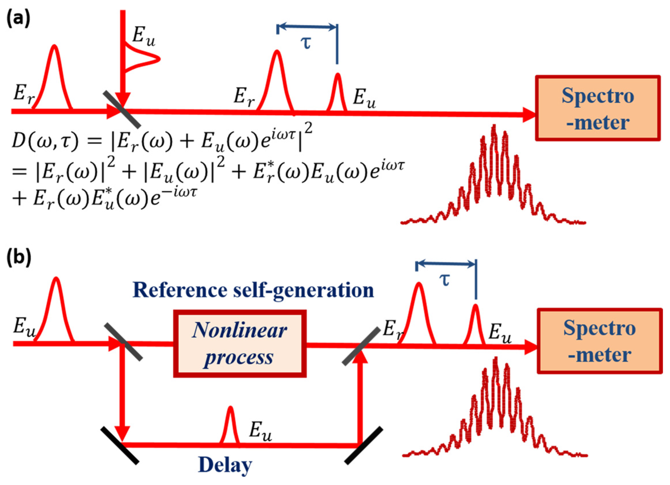
Nonlinear processes are required for most ultrashort-pulse measurements to perform time-gating in the sampling of short temporal segments of the pulses to be characterized [29,30,36,49]. This requirement increases the complexity of an ultrashort-pulse measurement system because of the need for suitable nonlinear media and relatively high peak power [49]. The use of a reference pulse with a known amplitude and phase in SI drastically simplifies the measurement with respect to the equipment needed and algorithm used [36,37]. The principle of SI is shown in Figure 1a. An unknown pulse and a reference pulse, separated by a suitable time delay τ, are collinearly guided into a spectrometer. A spectral interferogram that includes the phase information of both the reference and the unknown pulse is obtained and expressed as , where and are the spectra of the reference pulse and the unknown pulse and and are the spectral phase of the reference pulse and the unknown pulse. Fourier transform spectral interferometry (FTSI) is introduced into the SI process to determine the spectral phase of the pulse to be measured [36].
If and are the complex spectral amplitudes at angular frequency of the reference and the unknown pulse, respectively, then the interferogram obtained by the spectrometer is expressed as
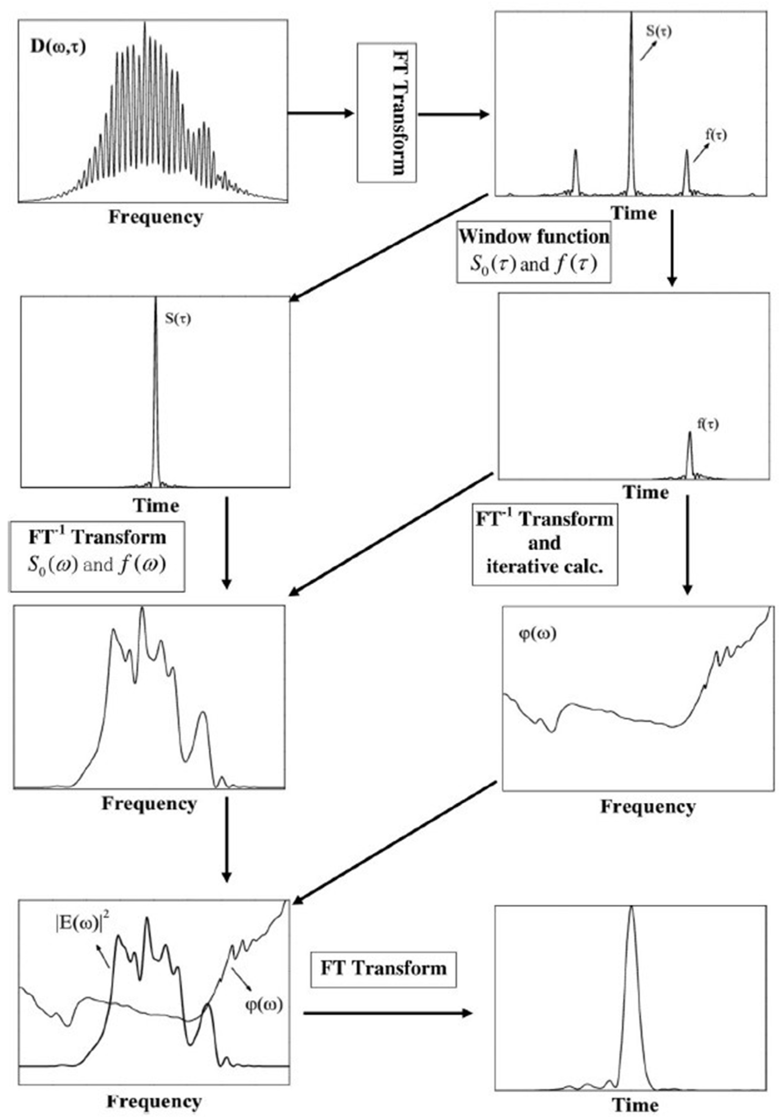
where is the sum of the spectral intensities of the reference and the unknown pulse and is the interference of the two spectra. The spectrum and spectral phase of the unknown pulse can be obtained using a Fourier transform-based procedure and an algebraic calculation, as outlined in the following steps and in Figure 2:
- (1)
- Fourier transform the interference signal from the frequency domain to the time domain and obtain the temporal signal containing and .
- (2)
- Separate and from the temporal signals obtained in Step 1 by using a suitable window function, e.g., a super Gaussian window. The width of the window function should be half of the gap between and (or half of the delay time between the reference pulse and the test pulse to be measured).
- (3)
- After inverse Fourier transforming and obtained in Step 2, we obtain the signals of and in the frequency domain, respectively.
- (4)
- Using and obtained in Step 3, the spectral amplitudes of the unknown pulse and the reference signal are analytically calculated using the following expressions [37]:
- (5)
- After calculating the phase using , the preliminary spectral phase of the pulse to be measured is calculated using Equation (4):where and are the spectral phases of the test pulse and the reference pulse, respectively.
- (6)
- Fourier transforming the laser spectrum obtained in Step 4 with the spectral phase obtained in Step 5 yields the temporal profile and duration of the pulse to be measured.
SI is a linear, analytical, sensitive, and accurate method for measuring ultrashort pulses [37]. By combining SI with FROG, a method named temporal analysis by dispersing a pair of light e fields (TADPOLE) was developed and demonstrated in 1996 [50]. Owing to the simplicity and linearity; hence, the high sensitivity of SI, TADPOLE can characterize the temporal profile of a pulse train with an average energy of 42 zJ (42 × 10−21 J) per pulse. Thus, SI can be used to measure the temporal contrast of a femtosecond laser pulse, as discussed in the following section. However, a separate FROG measurement makes this method very complicated.
Development of SRSI was driven by the recent research performed to improve the temporal contrast of the ultraintense femtosecond laser using the XPW method [51,52,53]. The generated XPW wave has a broadened and smoothed spectrum and a smoother and flatter spectral phase than that of the incident pulse because of the temporal filtering effect of the XPW process [35]. The principle of the SRSI method is presented in Figure 1b and described as follows: A reference pulse is self-created from a fraction of the input unknown pulse using a frequency-conserved nonlinear optical process. The self-created reference pulse and the input unknown pulse are then collinearly guided into a spectrometer with a time delay τ, which results in spectral interference in the spectrometer. The spectral phase of the generated reference pulse is almost flat in the entire spectral range, usually owing to the pulse-cleaning process if the pulse duration of the input unknown pulse is smaller than twice that of its Fourier-transform-limited pulse duration [37]. Then the spectral amplitude and phase of the input unknown pulse can be reconstructed from the spectral interference using the classical FTSI process presented in Figure 2. SRSI originated from SI; the main difference between the two is that, in the former, the reference pulse is generated from the incident pulse using frequency-conserved third-order nonlinear processes.
Previously, we assumed that the spectral phase of the generated XPW wave is absolutely flat or equal to zero. This assumption limits the application range of the SRSI method in measuring a pulse with low dispersion. The spectral bandwidth of the generated reference pulse is narrower than that of the incident pulse if the chirp of the incident pulse makes the duration of the unknown pulse broader than twice that of its Fourier-transform-limited pulse [33]. Furthermore, although the spectral phase of XPW is very flat, it usually is not equal to zero in the entire spectral range. To obtain a precise measurement of the spectral phase, an iterative calculation is performed as follows:
- (i)
- Using the expression , we obtain the temporal profile of the reference pulse using the temporal profile of the unknown pulse obtained in Step 6 above. After taking the inverse Fourier transform of , the spectrum and spectral phase of the reference pulse are obtained.
- (ii)
- The new spectral phase of the reference pulse, , is then used to find the new spectral phase of the test pulse, , where C is the constant spectral phase with respect to the wavelength induced by dispersive optics, such as that in a beamsplitter, and can be obtained by a simple calculation. After taking the Fourier transform of the laser spectrum of the test pulse by using the new spectral phase, we obtain a new temporal profile and pulse duration for the input unknown pulse.
- (iii)
- After performing Steps (i) and (ii) only three times, the corrected spectrum and spectral phase of the pulse to be measured are obtained, and the precise temporal profile and pulse duration are then obtained.
A correct measurement requires that the spectrum of the reference pulse created from a fraction of the input unknown pulse be broader than that of the input unknown pulse. Otherwise, the phase of some frequencies in the input pulse cannot be measured correctly [53,54]. The chirp of the input unknown pulses, which determines the bandwidth of the self-created reference pulses, is limited to twice the Fourier transform limit [35,37].
For a measurement to be correct in the SRSI method, the spectra of the reference pulses must be broader than those of the incident pulses, and the spectrum measured with the spectrometer and the spectrum reconstructed by the algorithm must be in good agreement. If not, the incident pulses may be unstable or too complicated with a chirp too large for this method [54].
3. Reference Pulse
An important step in the SRSI method is the generation of a reference pulse from the incident pulse using a frequency-conserved nonlinear process. Here, we consider how an appropriate reference pulse can be obtained.
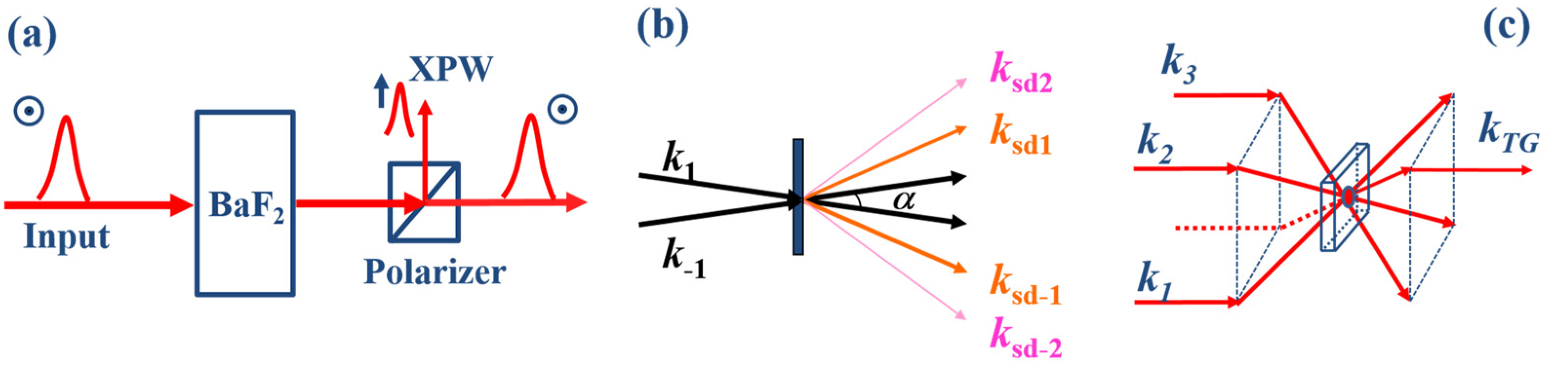
XPW, SD, and TG are all frequency-conserved four-wave-mixing processes that are used to improve the temporal contrast of ultrahigh-peak-power femtosecond laser systems [51,55,56]. The performances of the generated XPW wave, SD signal, and TG signal show that these processes satisfy the requirement as a reference pulse for the SRSI method. The principles of the XPW generation, SD, and TG processes are shown in Figure 3.
Figure 3a presents the principle of XPW. A linear polarized pulse is focused into a BaF2 crystal, generating an XPW wave with polarization perpendicular to that of the incident pulse. The generated XPW wave is separated from the incident pulse by placing a polarizer after the BaF2 crystal. XPW is a self-phase-matched, polarization-nondegenerate, frequency-degenerate four-wave-mixing process. Figure 3b shows that for the SD effect, two incident laser pulses from a single pulse are focused into a transparent medium with a small crossing angle, generating SD signals in addition to the two incident beams on the other side of the medium. Higher-order cascaded SD signals are also generated when the incident pulse energy is sufficiently high, because SD is a frequency-degenerated cascaded four-wave-mixing process [57]. Figure 3c presents the principle of the TG process, which requires three input laser beams, making the TG setup complicated. However, TG is a self-phase-matched process because a BOXCARS beam geometry is used [58]. Moreover, in comparison to the XPW and SD processes, TG is notably more sensitive to the incident pulse energy and thus can be extended to measure weak pulses [31].
XPW, SD, and TG are all third-order nonlinear processes. Therefore, the spectra and temporal profiles of the generated pulses are defined by the following equations:
The temporal profile of the generated signal is cleaned because its intensity is proportional to the cube of that of the incident pulse. In these very fast parametric processes, which have a response time of a few hundreds of femtoseconds, the temporal profile is cleaned within picoseconds. The spectrum and spectral phase of this kind of cleaned signal pulse are smoothed. Equation (6) shows that the spectrum of the generated reference pulse is smoothed and broadened because it is an integral (i.e., an average contribution) of the spectra of the incident pulses.
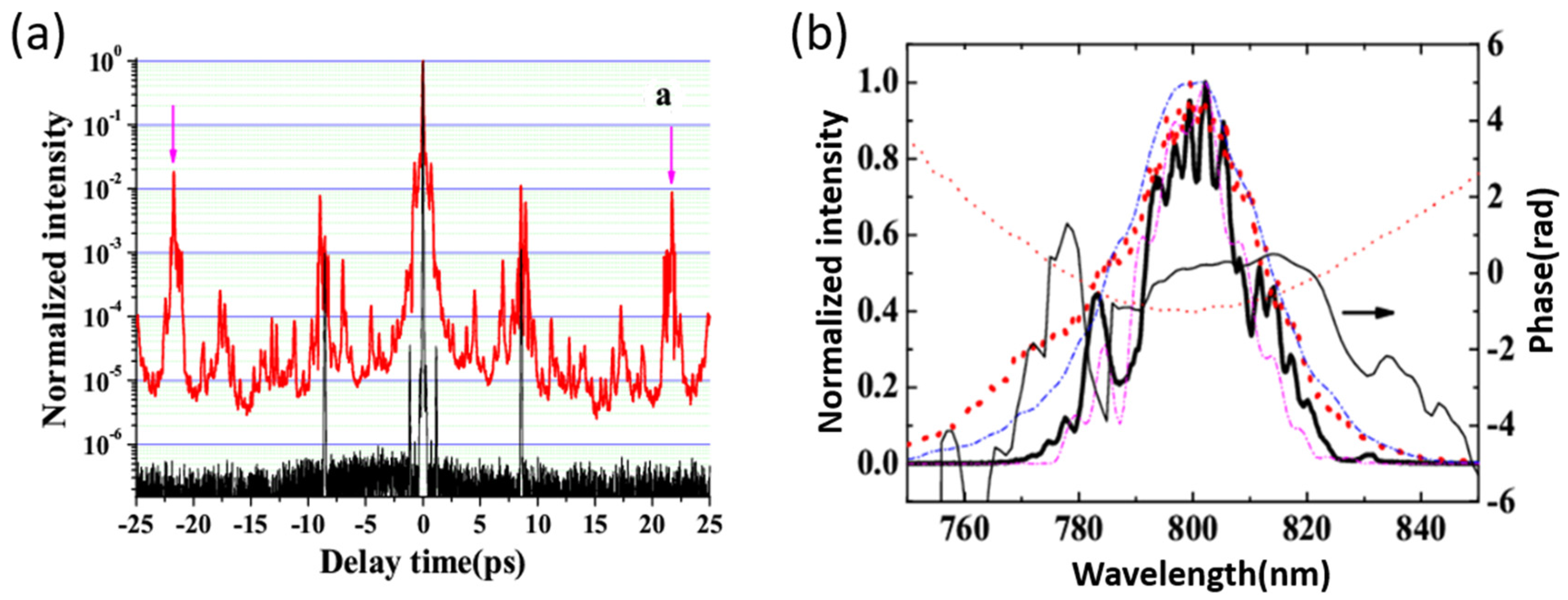
Figure 4a shows the typical improvement in the temporal contrast of the reference pulse compared to that of the incident pulse during the SD process. The temporal contrast of the SD signal was improved by four orders of magnitude. Figure 4b shows that the typical spectrum of the reference pulse (thick red dotted line) is broadened and smoothed in comparison to that of the incident pulse (thick black solid line). In addition, the spectral phase of the reference pulse (thin red dotted line) is smoothed and flattened in comparison to that of the incident pulse (thin black solid line).
4. SRSI for Temporal Profile Characterization
The three frequency-conserved thirdorder nonlinear processes XPW, SD, and TG for generating the reference pulse for the SRSI method that is used to characterize the temporal profile of femtosecond laser pulses are discussed in this section.
4.1. XPW-SRSI
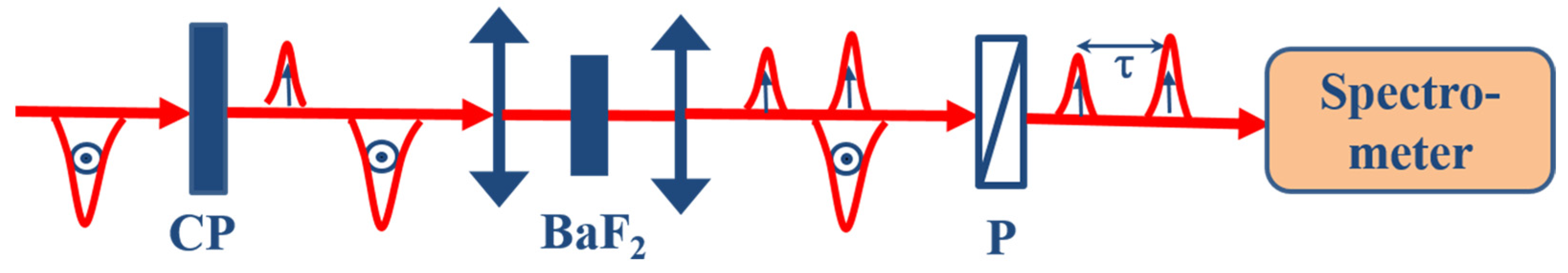
The XPW effect was the first third-order nonlinear process used in the SRSI method in which a single incident beam is used [31]. Figure 5 presents the principle of XPW-SRSI. In brief, a linear polarized unknown femtosecond laser beam passes through a calcite plate (CP) by which the polarization of a small fraction of the incident pulse becomes perpendicular with a time delay proportional to the thickness of the calcite plate. The incident pulse is then focused onto a BaF2 crystal to generate an XPW signal also with polarization perpendicular to that of the incident laser beam. Finally, a polarizer (P) separates the polarization-rotated incident pulse and the XPW signal. A spectrometer measures the spectral interference.
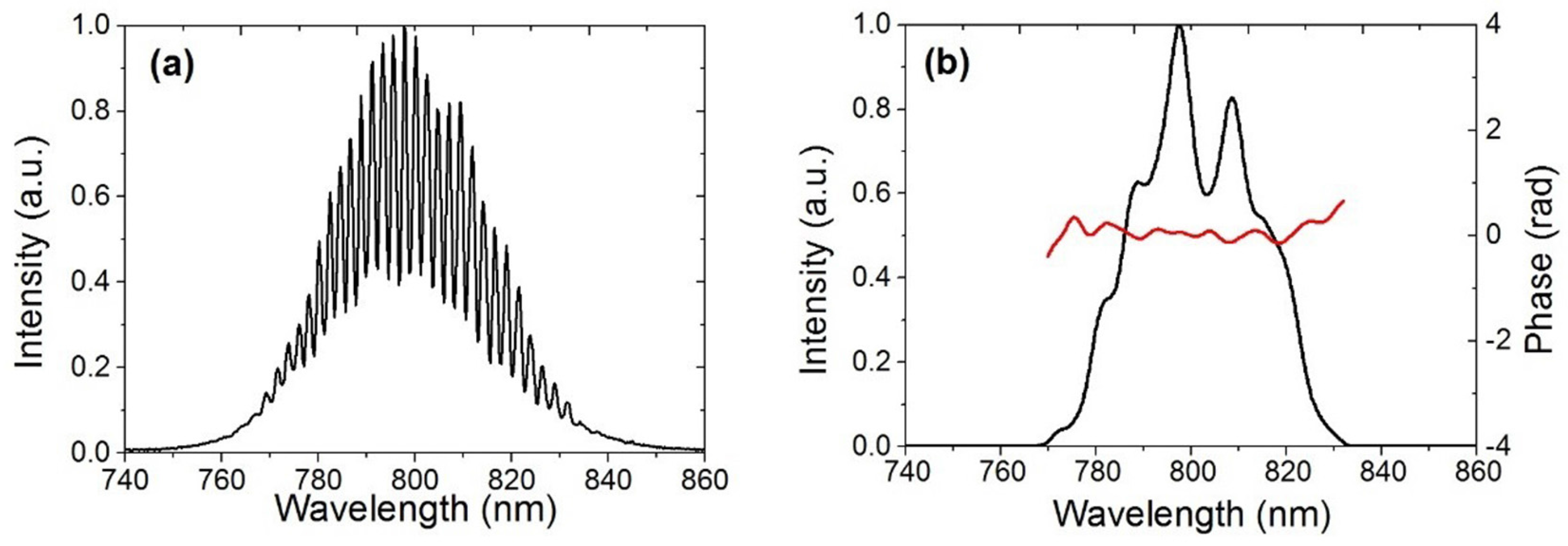
XPW-SRSI has two advantages over other methods: (1) It needs only one input beam, which simplifies its setup and alignment; and (2) the XPW process is a self-phase-matched process, which makes it suitable for broadband spectrum laser pulses. These two advantages have spurred much research in the past few years [40,41,42,54]. A laser pulse as short as 4 fs has been measured successfully using a low-dispersion optical setup [37]. A dynamic range up to 50 dB with a ±400 fs window was characterized using a common 25 dB SNR spectrometer [35]. A commercial femtosecond pulse measurement device named Wizzler (FASTLITE, Paris, France) has been used by some groups to characterize laser pulses. Figure 6 shows a reconstructed spectrum and spectral phase of a laser pulse obtained by Wizzler in the laboratory.
4.2. SD-SRSI
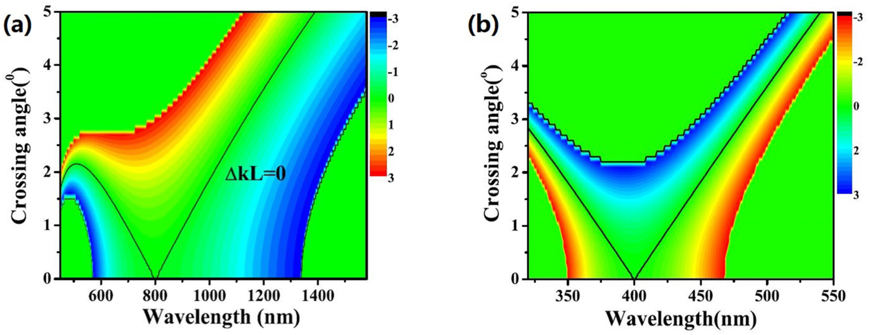
Although XPW is used in the SRSI method with success, the polarizer limits the spectral range and usually induces dispersion of the incident pulse. This limitation is the same as that which occurs when the XPW effect is used in pulse cleaning, where the polarizer limits the improvement of the temporal contrast because of its extinction ratio. Recently, a reflective polarizer was used in the XPW-SRSI method to solve this problem [31]. In 2010, we used the SD process, which does not require a polarizer, to obtain greater improvement in the temporal contrast [51]. As with pulse cleaning, the limitation caused by a polarizer can be eliminated if the SD effect is used in the SRSI method, because a polarizer is not used. The SD process is a non-collinear four-wave-mixing parametric process and not a self-phase-matched process. A relatively thin nonlinear medium should be chosen to satisfy the broadband phase-matching of the SD process. The two-dimensional phase-matching patterns of SD processes at 800 nm in a 0.1-mm-thick fused silica glass plate and at 400 nm in a 0.1-mm-thick CaF2 plate are shown in Figure 7a,b, respectively. The phase-matched spectral range is wider than nearly one octave at 800 nm, which can support the characterization of sub-5 fs laser pulses.
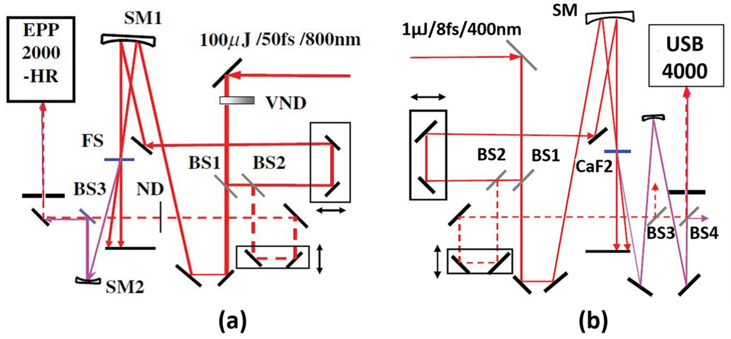
Experiments were performed to show the principle with the center wavelength of the pulse at 800 and 400 nm. In the experimental setups shown in Figure 8, beamsplitter BS2 is used to separate a test pulse. The generated SD reference pulse is collinearly combined with the test pulse by another beamsplitter.
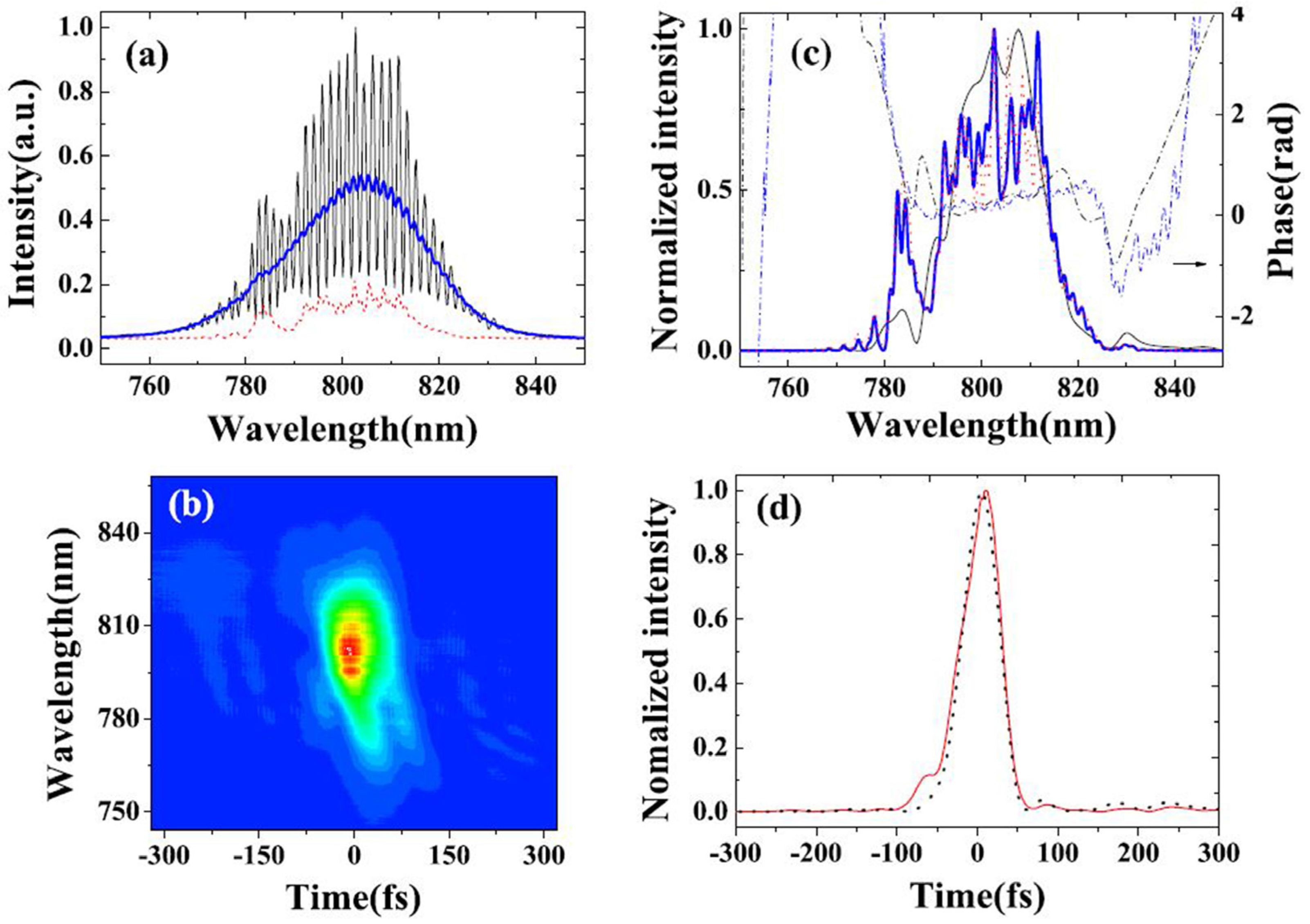
Figure 9 and Figure 10 show the results obtained using the setups displayed in Figure 8 at 800 and 400 nm, respectively. Figure 9a,b show the original data obtained in the experiment using SD-SRSI and SD-FROG, respectively, for a pulse at 800 nm. Figure 9c shows the resulting spectra and spectral phases of the test pulse obtained by SD-SRSI and SD-FROG, where the reconstructed spectrum obtained by SD-SRSI agrees well with the spectrum measured directly by the spectrometer; even the fine spectral modulation overlaps. Figure 9d shows that the reconstructed pulse profiles for both methods closely overlap, with a pulse duration of ~55 fs for both closed temporal profiles.
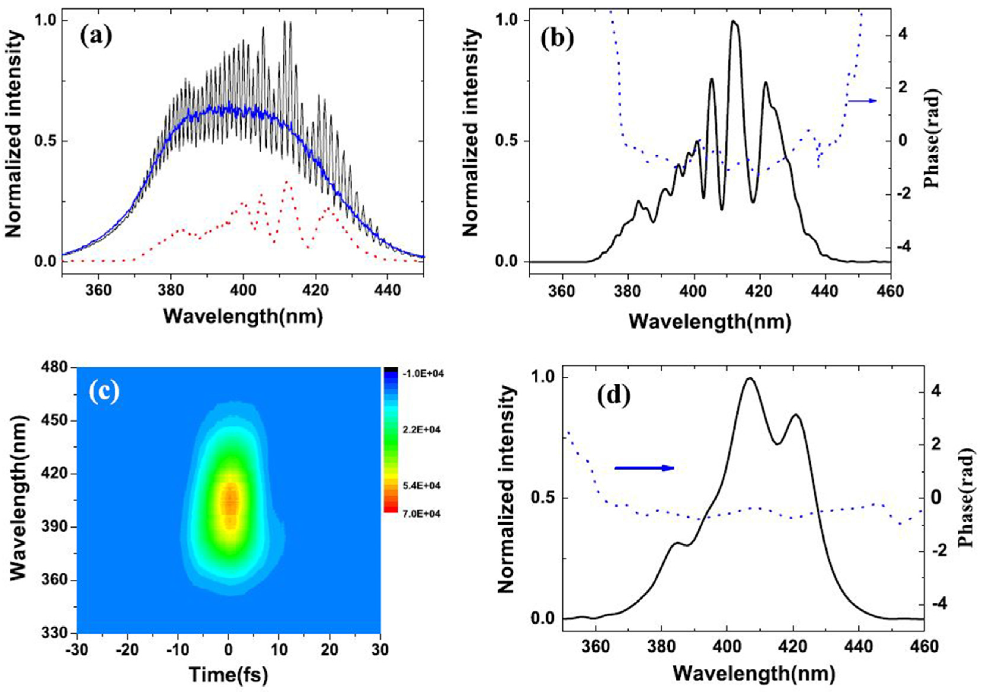
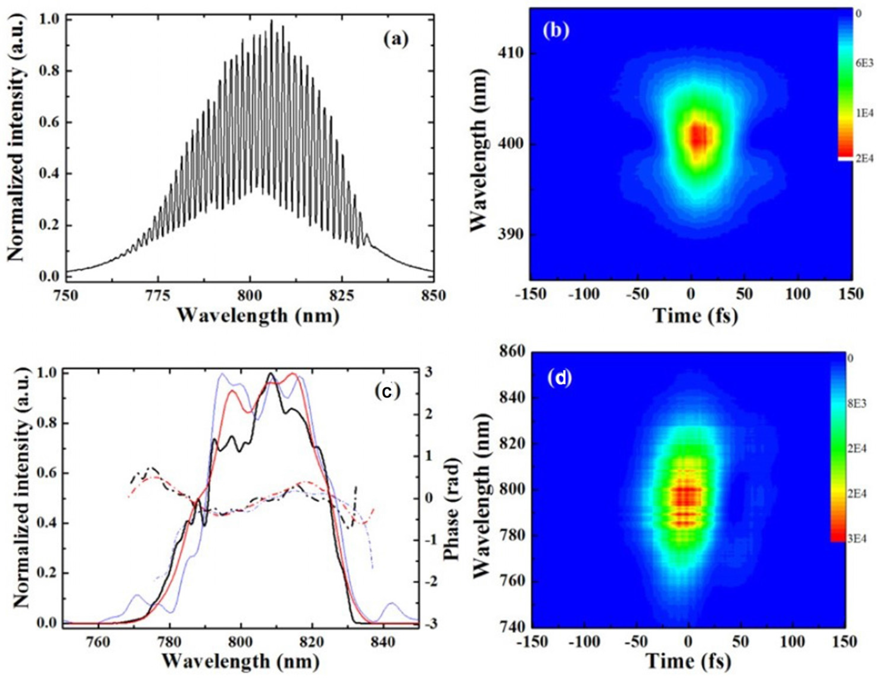
Figure 10a,b show the original data obtained by SD-SRSI and SD-FROG measurements of a sub-10 fs pulse at 400 nm. Figure 10c,d show the reconstructed spectra and spectral phase of the unknown pulse obtained by SD-SRSI and SD-FROG, respectively. Even a sub-10 fs pulse at 400 nm can be measured using this setup. However, the setup is complex, because three beamsplitters are necessary to split the beam into three beams. We simplified the setup by using simple fixed holes to split the beam into three [59].
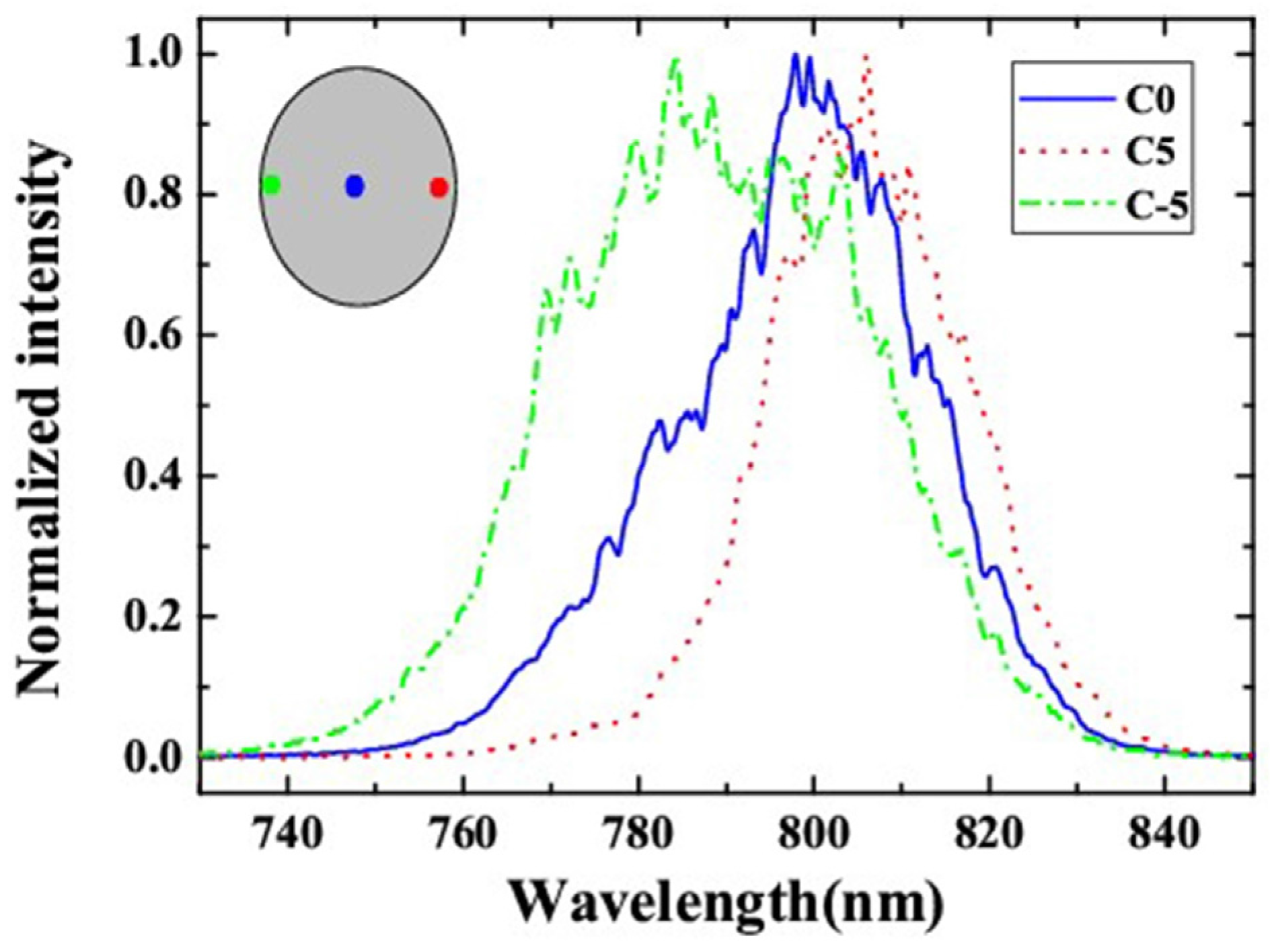
Experiments showed that the SD signal has an obvious angular chirp because SD is a non-collinear optical parametric process that needs to satisfy the phase-matching condition. Figure 11 shows a typical angular chirp of an SD signal. If a different part of the SD signal is selected for the reference pulse, its angular chirp makes the spectrum of the reference pulse different, which will introduce error into the measured result. This angular chirp is not easy to remove in the SD process.
Compared to the XPW-SRSI method, the SD-SRSI method has the following disadvantages: (1) The SD process requires a phase-matching relationship and a relatively thin nonlinear medium, whereas the XPW process is self-phase-matched; (2) the SD process needs a non-collinear geometry and two incident beams, which makes the system more complicated. In addition, the two beams must be carefully aligned and stably synchronized; (3) because the SD process requires a thin nonlinear medium and a non-collinear geometry, its efficiency is expected to be lower than that of XPW for the same beam and pulse parameters. On the other hand, the SD-SRSI method has the following advantages: (1) The SD-SRSI method is less limited in the spectral range and pulse duration because no polarizer is used. Therefore, it can be used to measure a shorter pulse in a broader spectral range, from UV to middle IR, using one optical setup; (2) by using SD-FROG measurement, it can simultaneously be used to measure pulse duration with a relatively large chirp; this cannot be done using the XPW-SRSI method; (3) because the SD effect appears in all third-order nonlinear media, birefringence does not need consideration. An incident pulse with lower energy should operate in a higher third-order nonlinear medium.
4.3. TG-SRSI
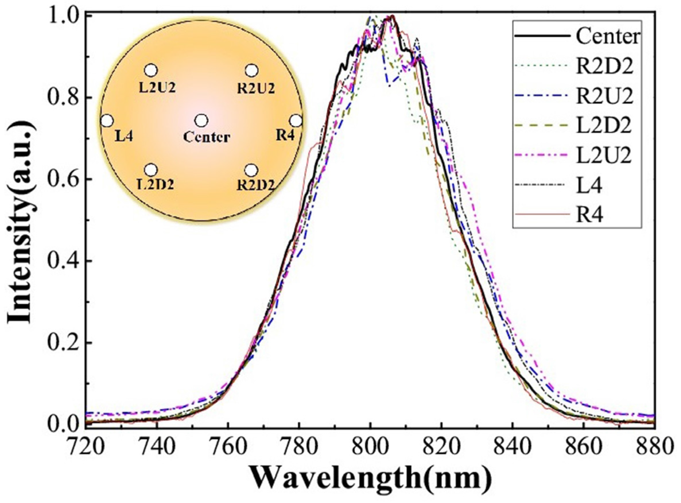
XPW-SRSI is limited by the polarizer and SD-SRSI is limited by the phase-matching or angular chirp of the SD signal. How can these problems be solved? The TG effect is also a frequency-conserved third-order nonlinear process that has been used in ultrashort TG spectroscopy and TG-FROG pulse characterization. The TG process is self-phase-matching and does not require a polarizer. Moreover, the TG signal has no spatial or angular chirp, as shown in Figure 12, in which all the spectra have nearly the same profile, indicating negligible angular dispersion in the generated TG signal. Furthermore, there was no obvious angular dispersion when the crossing angle increased from 2° to 6° during the TG process in a 500-μm-thick fused silica plate.
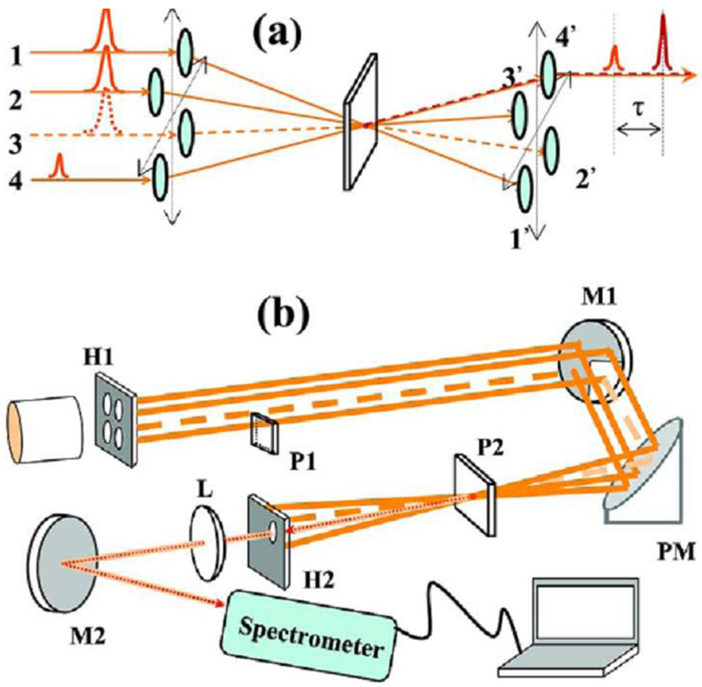
These properties make TG suitable for use with the SRSI method, and the polarizer and angular chirp limitations of XPW-SRSI and SD-SRSI, respectively, are avoided. The principle of TG-SRSI is shown in Figure 13a. The unknown pulse to be characterized is separated into four beams, one of which is energy-attenuated, time-delayed, and then used as the testing beam. It and the other three beams are focused onto a thin transparent plate in a BOXCARS beam geometry and the three beams overlap in time and space. The TG signal is generated in the same direction as the testing beam so the optical setup of this system is alignment-free.
A simple experimental setup based on the principle of TG is composed of only a few optical components, as shown in Figure 13b. A black plate (H1) with four equal-sized holes separates the incident beam into four beams. A 500-μm-thick fused silica plate (P1) is placed in the path of the testing beam to induce a suitable delay between it and the other three beams. The delay can be adjusted by simply rotating P1. A specially designed plane mirror (M1), three-fourths of which is coated with protective silver, is used to attenuate the testing beam. The reflectivity of the uncoated part of M1 is calculated to be about 0.6% for horizontally polarized light and an incident angle of 45°. A silver-coated parabolic mirror (PM) focuses the four beams onto a second 500-μm-thick fused silica plate (P2) to generate the TG signal. To avoid any distortion by other third-order nonlinear processes, the incident pulse energy is sufficiently low, which makes the efficiency of the TG signal <1%. An iris (H2) selects the combined TG signal and testing beam, which is then focused into a spectrometer (AvaSpec UL3648-USB2, Avantes, Apeldoorn, The Netherlands). A spectral interferogram is obtained when the delay between the TG signal and the testing pulse is ~1000 fs. Thus, the temporal profile of the testing pulse can be obtained in real-time or in a single shot.
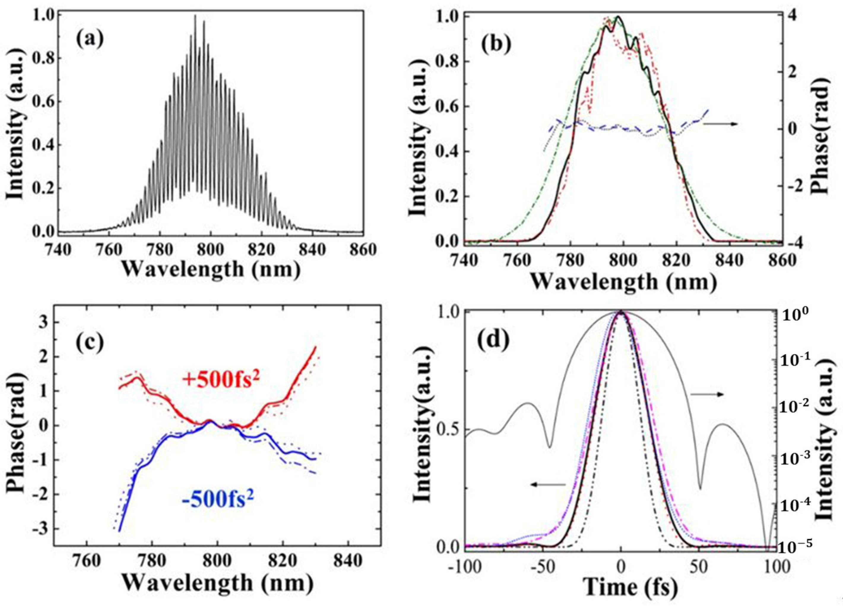
The original measured spectral interferogram obtained using the TG-SRSI setup is shown in Figure 14a. Figure 14b shows that the flat spectral phase, reconstructed on the basis of the spectral interferogram, overlapped well with the spectral phase obtained by Wizzler. To prove further the reliability of the TG-SRSI technique and setup, precise 500 fs2 and −500 fs2 group delay dispersions (GDDs), induced by a Dazzler ultrafast pulse shaper (FASTLITE), were added directly to the incident pulse. Figure 14c shows the chirped spectral phases of the testing pulse with the ±500 fs2 GDDs added as measured by TG-SRSI and Wizzler, and the calculated spectral phase obtained by adding ±500 fs2 GDD onto the flat phase in Figure 14b. The figure shows that all three spectral phases coincide. These results prove that TG-SRSI used in our simple setup can accurately characterize femtosecond pulses. Figure 14d shows the reconstructed temporal profiles of the testing pulse after adding 0, 500, and −500 fs2 GDDs to the incident pulse. The resulting pulse durations (hereafter referred to as mean FWHM) were 37.5, 42.1 and 42.6 fs, respectively, when the testing-pulse and the TG reference signal had the Fourier-transform-limited (FTL) pulse durations of 36.8 and 27.0 fs, respectively. Moreover, the temporal profile of the 37.5 fs testing pulse had a 50 dB dynamic range.
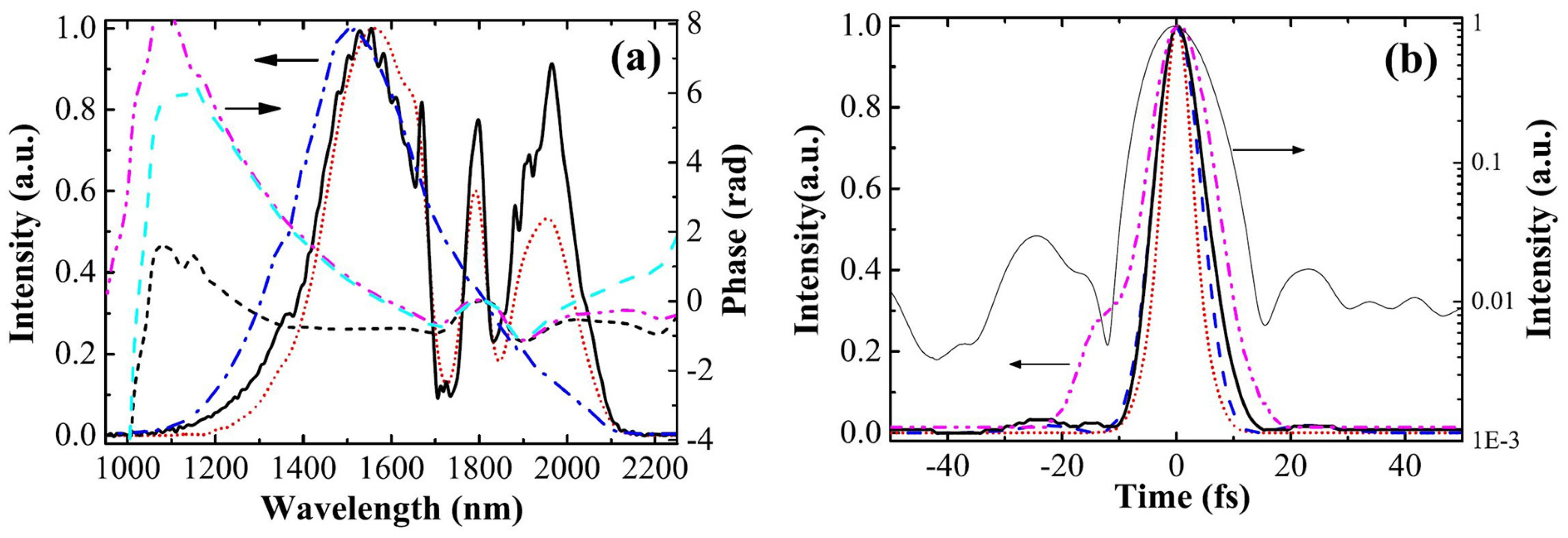
In the TG-SRSI method, the nonlinear medium is an arbitrarily selected transparent plate. In principle, the TG-SRSI method can be used to characterize femtosecond pulses at other wavelengths by replacing the spectrometer with one suitable for the test pulse. To check the potential of the TG-SRSI method and our setup, a sub-10 fs pulse with a center wavelength of approximately 1.8 μm was tested using the setup shown in Figure 13b, where only the spectrometer was changed (NIR256-2.1, Ocean Optics, Dunedin, FL, USA). Figure 15 shows the results of the characterization experiment. The spectrum of the laser beam, measured directly by the spectrometer, was close in shape to that of the TG-SRSI-reconstructed spectrum, as seen in Figure 15a; the corresponding reconstructed spectral phase is also shown. Placing a 1-mm-thick fused silica plate at the Brewster angle before the setup for dispersion compensation obtained the shortest pulse of 10.6 fs, as shown in Figure 15b on linear and logarithmic scales. Because the spectral range of the NIR256-2.1 spectrometer is limited, a signal longer than 2.1 μm cannot be measured. It is not clear why the intensity of the longer-wavelength TG signal is always weak. The FTL pulse duration of the TG signal was 6.8 fs, which is much shorter than that of the testing pulse at 9.6 fs, as shown in Figure 15b. To investigate the reliability of the measurement, the 1-mm-thick fused silica plate was removed, inducing −55 fs2 and 250 fs3 dispersions at this wavelength to the pulse. Therefore, the pulse was broadened to 15.1 fs because of the uncompensated dispersion. The reconstructed spectral phase coincided with the calculated spectral phase, as seen in Figure 15a. This result clearly proves that the TG-SRSI method is capable of working and yielding reliable results in the mid-IR spectral region.
Although SRSI works well in characterizing femtosecond pulses, its one drawback is the requirement that a broadened reference spectrum be generated by the third-order nonlinear process, which may result in the generation of a reference pulse with a narrower spectrum than that of the testing pulse. This typically occurs when the femtosecond pulses (especially pulses with few cycles) to be characterized have a large chirp [35,37]. Because of the two requirements of SRSI, it will not work correctly under these conditions. The SRSI method will work well only for femtosecond pulses with small chirp, which will provide a broadened spectrum of the generated reference signal. Thus, all independent methods for femtosecond pulse characterization have their own advantages and disadvantages when their properties are compared. The application of each method and its corresponding setup has a limited spectral or temporal range. The disadvantages and the advantages of FROG and SRSI are complementary. FROG is energy-sensitive and capable of characterizing pulses with large chirp, even complex pulses, while SRSI is a fast method with a simple setup. Furthermore, SD and TG processes can be used with both methods. Therefore, if the two methods are combined using the SD or the TG process, a method with the most advantages and a wider application range is obtained. We call this method FASI (Frequency-resolved optical gating And Self-referenced spectral Interferometry) [61].
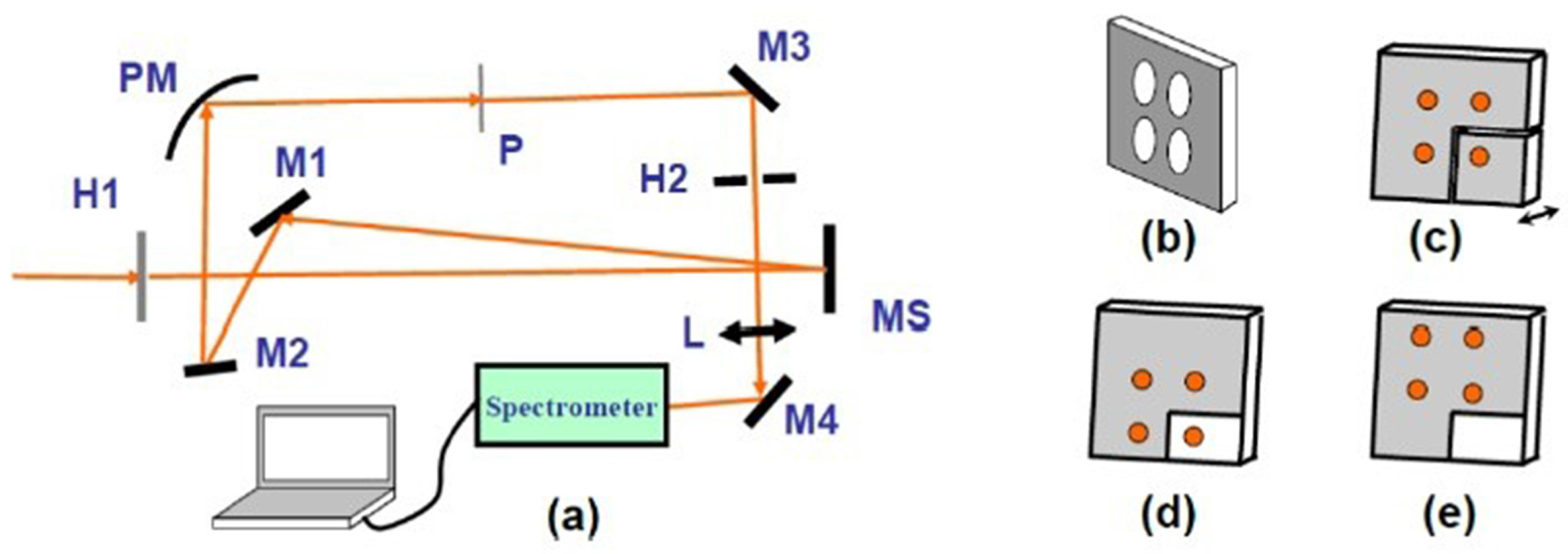
The experimental setup used to prove the capability of the FASI method in practical use is shown in Figure 16a. A variable neutral density filter is used to continuously change the incident pulse energy before entering the setup. A black plate (H1) with four equal-sized holes is used to separate the incident beam into four 2.5-mm-diameter beams. The four holes are arranged in a rectangle and form BOXCARS geometry. The four beams are introduced into a mirror set (MS) comprising an L-shaped mirror and a separate square mirror, which fits into the L-shaped mirror, as shown in Figure 16c. The square mirror, connected to a motorized stage (M-122, PI), introduces scanned or fixed delay for FROG or SRSI, respectively. The mirror set reflects the four beams to a specially designed mirror (M1), of which five-sixths of its area is silver-coated and one-sixth of the left part is not coated, as shown in Figure 16d,e. M1 is fixed on a manual stage that can be moved vertically. For TG-FROG measurements, M1 is moved down and all four beams are reflected by silver-coated part of the mirror, as shown in Figure 16e. For SHG-FROG or TG-FROG measurements, only two or three beams, respectively, are needed. For TG-SRSI measurements, M1 is moved up, and the beam reflected by the quarter mirror (Figure 16c) is reflected again by the uncoated part of M1 (Figure 16d). M1 reflects all the beams onto M2 at a reflective angle of ~50°. Using the Fresnel equation, the reflectivity of the uncoated part of M1 is calculated to be <0.3% for horizontally polarized light. Thus, the testing-pulse energy will be reduced to result in perfect spectral interference. M2 reflects the beams onto a silver-coated parabolic reflector (PM), with a focal length of 150 mm, which focuses all the beams onto a 500-μm-thick fused silica plate (P) to generate the TG signal. For SHG-FROG measurements, the upper two beams on M1 are blocked and the glass plate is replaced by a 50-μm-thick beta barium borate (BBO) crystal. For TG-SRSI measurements, the TG signal and the test beam are collinearly self-combined and pass through an iris (H2). For TG-FROG and SHG-FROG measurements, only the TG and the SHG signal, respectively, is selected by the iris. The selected signals are focused by a focal lens (L) onto a plane mirror (M4) before entering a spectrometer to acquire the original data.
Using the FASI setup with the TG-SRSI, TG-FROG, and SHG-FROG methods, we independently characterized an ~40 fs pulse at 800 nm from a Ti/sapphire laser system. In this setup, TG-SRSI is fast, TG-FROG is suitable for complex pulses and a wide spectral range, and SHG-FROG is energy-sensitive. The results obtained by these three methods are shown in Figure 17, where they are compared to prove the reliability of the FASI method. The original spectral interferometry and two-dimensional frequency‑time spectrogram obtained using TG-SRSI, SHG-FROG, and TG-FROG are shown in Figure 17a,b,d, respectively. The spectral interferometry data were obtained in single-shot when the delay between the TG signal and the test beam was ~1.3 ps. Thus, for many laser systems, our FASI device can run in real-time or single-shot condition when in TG-SRSI mode. The SHG-FROG and TG-FROG data were collected by using the motorized stage to scan for 256 steps at 2 fs per step. Figure 17c shows the reconstructed spectra and spectral phases obtained by the three methods. The reconstructed spectrum of TG-SRSI showed the best fidelity, owing to the analytical calculation. The reconstructed spectral phases of the three methods overlapped each other well. These results clearly prove the ability to combine FROG and SRSI in a single setup by using the TG effect. This combination also promises that the FASI device will be reliable and consistent with the three methods. In addition, this device can be extended to the UV and MIR spectral range because the TG effect is not limited by the phase-matching requirement.
Weak femtosecond pulses (sub- to several nanojoules) generated by oscillators or non-collinear optical parametric amplifiers are widely used to explore ultrafast phenomena in biology and chemistry. Accurate and complete temporal characterization of such pulses is vitally important in these applications. SHG-FROG is used in the FASI setup for energy-sensitive pulse characterization because SRSI is based on a third-order nonlinear process, which usually needs pulses at the microjoule level as input. However, for SHG to be efficient in real use requires a phase-matching process, which limits the spectral range. Can SRSI be used to characterize sub-nanojoule femtosecond pulses? The answer is yes, as outlined below.
To extend the use of the SRSI method for weak-pulse characterization, we explored the TG-SRSI technique because the TG process is relatively sensitive to higher energy compared to the SD and XPW processes [31], as shown in Table 1. Femtosecond pulses of <100 nJ had been successfully characterized on the basis of a reflective objective design using TG-SRSI [62]. However, that energy level is still far from sub-nanojoule level, so TG-SRSI cannot be used to characterize femtosecond pulses from oscillators. How can the TG-SRSI method be improved to measure a sub-nanojoule femtosecond pulse? In addition, a relatively compact device with a high performance level like that of a sensor would be powerful in the application of TG-SRSI. How can we simplify the optical setup to achieve such a device?
There are three key points for the successful characterization of sub-nanojoule femtosecond pulses using an optical setup that is smaller than a palm. (1) Use the TG process, with its sensitivity to higher energy levels, to generate the reference pulse. (2) Use a nonlinear medium with relatively higher third-order nonlinearity. (3) Most importantly, use a symmetric focusing and collimation pair of parabolic mirrors with a tight focal length to make the focal intensity in the nonlinear medium as high as possible. The use of a symmetric pair of parabolic mirrors will simplify the setup and make it easy to align.
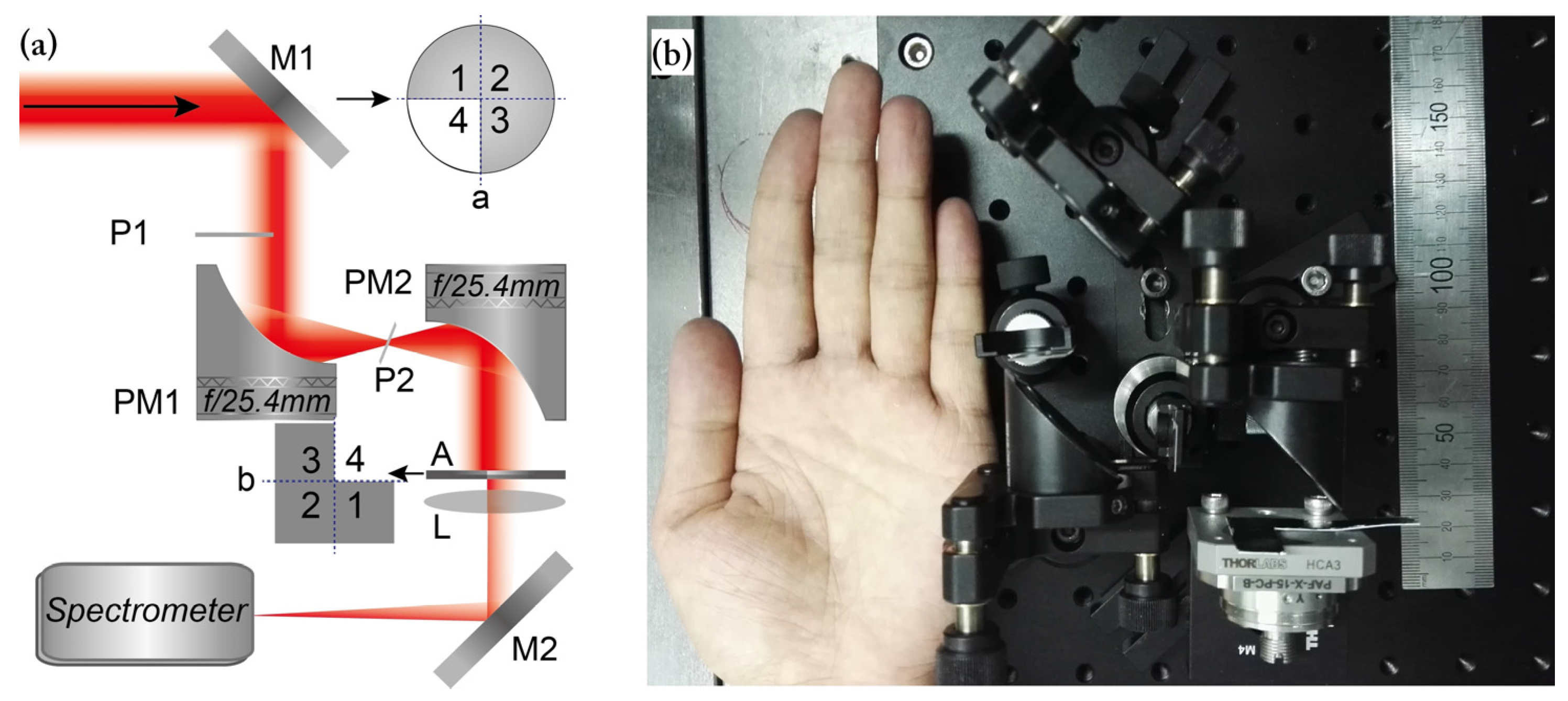
The enhanced TG-SRSI setup is shown in Figure 18a. The input unknown pulse is reflected by a special coated mirror (M1), of which three-fourths of its front surface has a high reflectivity coating and the remaining area is not coated, as shown in the inset “a” of Figure 18a. The input unknown laser beam can be regarded as four beams, , , and , which are reflected from areas 1, 2, 3 and 4 of M1, respectively. The first three beams are identical incident beams that generate the TG reference beam, and , which is dramatically attenuated by the uncoated glass surface, is used as the testing pulse to be calculated. An off-axis parabolic aluminum mirror (PM1), with an effective focal length of only 25.4 mm, focuses the four beams. When , , and are focused by PM1 into a nonlinear 0.15-mm-thick YAG plate (P2) simultaneously, a TG reference pulse is generated owing to the TG nonlinear process. Beam , the input unknown pulse denoted as , is attenuated by the uncoated area of M1 when the incident angle of the p-polarized unknown pulse on M1 is ~45°. A 0.5-mm-thick fused silica plate (P1) is inserted in the propagation path of to introduce a time delay τ between and . P1 can attenuate to a certain value when its coating film has a different reflective ratio. After P2, another off-axis parabolic aluminum mirror (PM2), with the same 25.4-mm effective focal length as PM1, symmetrically collimates the beam. Beams and are automatically in the same direction owing to the BOXCARS beam geometry of the TG process [60,62]. Both the symmetric parabolic mirrors pair and the BOXCARS geometry make the setup easy to align. and , with a time delay τ between them, are filtered out and guided into a spectrometer by a lens (L) and a high reflectivity mirror (M2).
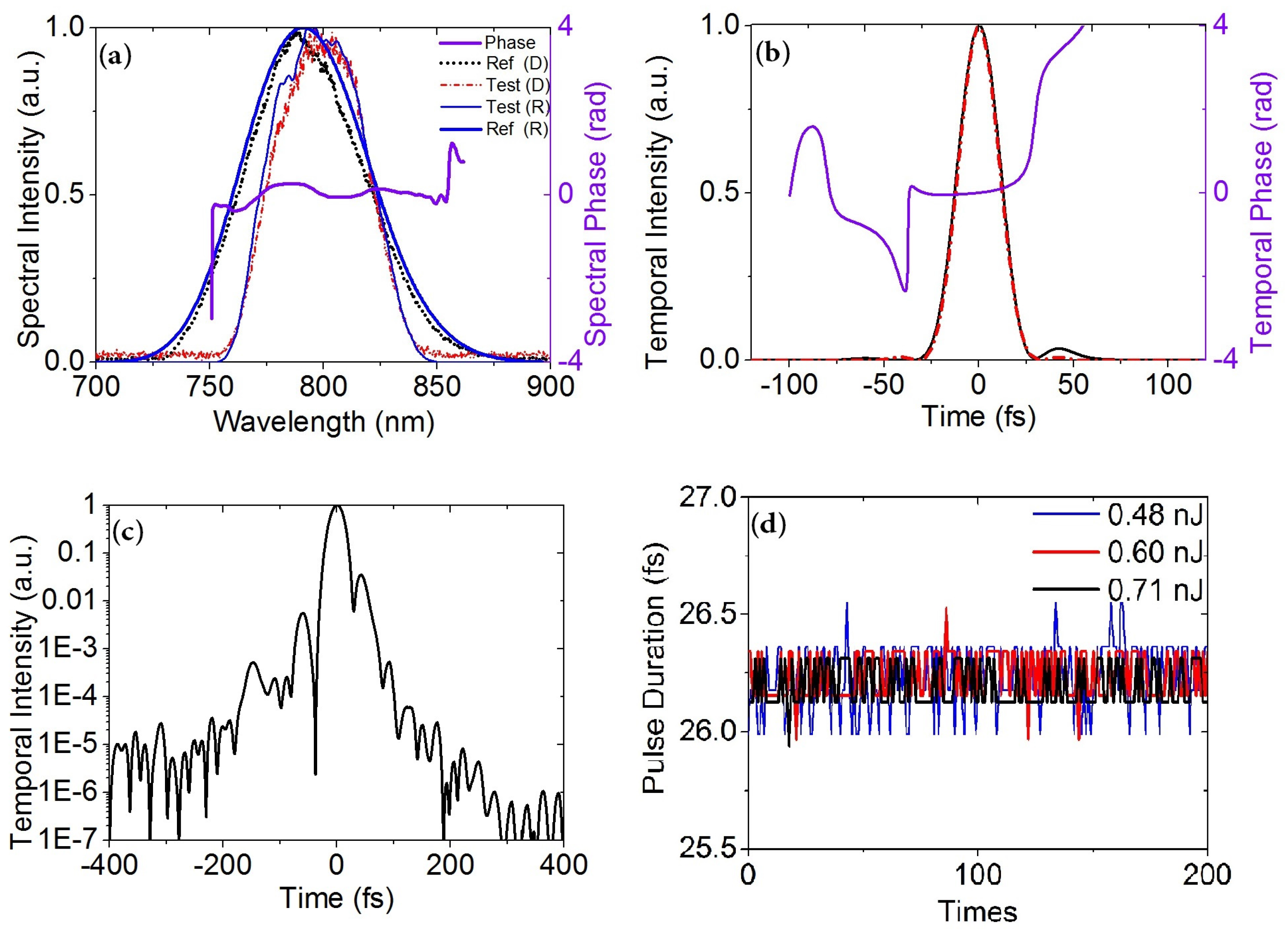
Figure 19 presents the results of measuring 0.48, 0.60, and 0.71 nJ pulses with the enhanced TG-SRSI. The reconstructed spectra and the spectra directly measured by the spectrometer match very well, as seen in Figure 19a. The spectrum of the self-created reference pulse is broader and smoother than that of the input unknown pulse, which proves the reliability of measurements obtained with this setup. Figure 19b shows the reconstructed temporal profile and phase of the 0.48 nJ input unknown pulse, which had a pulse duration of about 26.3 fs. The reconstructed temporal profile on a logarithmic scale (Figure 19c) shows a 50 dB dynamic range on a ±400 fs temporal range. Figure 19d shows the fluctuation in pulse duration in the characterization results for 0.48, 0.60, and 0.71 nJ pulses. Each curve consists of 200 measured results. The results presented in Figure 19 prove the reliability of the pulse characterization measurements obtained with the enhanced TG-SRSI setup, even at pulse energies <0.5 nJ per incident pulse. Thus, we succeeded in extending the TG-SRSI method for use in characterizing sub-nanojoule pulses.
5. Discussion and Prospect
We have discussed several methods for characterizing femtosecond pulses. As a relatively novel method, SRSI has many advantages over other methods used to characterize the temporal profile of femtosecond laser pulses. The frequency-conserved third-order nonlinear processes XPW, SD, and TG are used to generate the reference pulse for SRSI, of which TG is the most advantageous. The combination of TG-FROG and TG-SRSI comprises the best properties for pulse measurement. Great progress has been made in improving SRSI, including extending the spectral range, improving its sensitivity to input pulse energy, simplifying the setup, and increasing the dynamic range. We hope to develop microdevices based on TG-SRSI similar to sensors that can be located inside a femtosecond laser system to monitor or control via feedback the temporal profile of output pulses.
SI can characterize pulses with an average energy of 42 zJ per pulse, i.e., less than one photon per pulse [50]. Furthermore, SRSI with a 25 dB SNR spectrometer can characterize a temporal profile with a 50 dB dynamic range during pulse measurement [39]. These properties allow SRSI to be used for the single-shot characterization of the temporal contrast of ultraintense femtosecond laser pulses. In 2013, researchers achieved a temporal contrast of up to 60 dB in a 25 ps window using SRSI [64]. However, this dynamic range is far lower than that required for the single-shot characterization of an ultraintense femtosecond laser pulse. We expect to extend the use of SRSI to the single-shot characterization of a femtosecond laser pulse with a considerably higher dynamic range. This should be possible, because the temporal resolution of SRSI is significantly higher than that of the third-order correlator, the temporal contrast resolution of which is usually hundreds of femtoseconds, or picoseconds. For a PW femtosecond laser system, with a pulse duration typically of tens of femtoseconds, precisely showing the satellite prepulses of the ultraintense laser by SRSI may assist in building or using such systems.
Acknowledgments
This work was supported by the National Natural Science Foundation of China (NSFC) (grants 11274327, 61521093, and 61527821), the Instrument Developing Project of the Chinese Academy of Sciences (grant YZ201538), and the Strategic Priority Research Program of the Chinese Academy of Sciences (grant XDB160106).
Author Contributions
J.L. conceived and designed the experiments; X.S., P.W., and J.L. performed the experiments and analyzed the data; and J.L., T.K., and R.L. supervised the project. All authors contributed to the preparation of the paper.
Conflicts of Interest
The authors declare no conflict of interest. The founding sponsors had no role in the design of the study; collection, analyses, or interpretation of the data; writing of the manuscript; or the decision to publish the results.
References
- Spielmann, C.; Burnett, N.H.; Sartania, S.; Koppitsch, R.; Schnurer, M.; Kan, C.; Lenzner, M.; Wobrauschek, P.; Krausz, F. Generation of coherent X-rays in the water window using 5-femtosecond laser pulses. Science 1997, 278, 661–664. [Google Scholar] [CrossRef]
- Durfee, C.G.; Backus, S.; Kapteyn, H.C.; Murnane, M.M. Intense 8 fs pulse generation in the deep ultraviolet. Opt. Lett. 1999, 24, 697–699. [Google Scholar] [CrossRef] [PubMed]
- Chang, Z.H.; Rundquist, A.; Wang, H.W.; Murnane, M.M.; Kapteyn, H.C. Generation of coherent soft X-rays at 2.7 nm using high harmonics. Phys. Rev. Lett. 1997, 79, 2967–2970. [Google Scholar] [CrossRef]
- Backus, S.; Peatross, J.; Zeek, Z.; Rundquist, A.; Taft, G.; Murnane, M.M.; Kapteyn, H.C. 16 fs, 1-mu j ultraviolet pulses generated by third-harmonic conversion in air. Opt. Lett. 1996, 21, 665–667. [Google Scholar] [CrossRef] [PubMed]
- Gale, G.M.; Gallot, G.; Hache, F.; Sander, R. Generation of intense highly coherent femtosecond pulses in the mid infrared. Opt. Lett. 1997, 22, 1253–1255. [Google Scholar] [CrossRef] [PubMed]
- Xu, L.; Zhang, X.C.; Auston, D.H. Terahertz beam generation by femtosecond optical pulses in electrooptic materials. Appl. Phys. Lett. 1992, 61, 1784–1786. [Google Scholar] [CrossRef]
- Wang, P.; Liu, J.; Li, F.; Shen, X.; Li, R. Multicolored sideband generation based on cascaded four-wave mixing with the assistance of spectral broadening in multiple thin plates. Photonics Res. 2015, 3, 210–213. [Google Scholar] [CrossRef]
- Schenkel, B.; Biegert, J.; Keller, U.; Vozzi, C.; Nisoli, M.; Sansone, G.; Stagira, S.; De Silvestri, S.; Svelto, O. Generation of 3.8 fs pulses from adaptive compression of a cascaded hollow fiber supercontinuum. Opt. Lett. 2003, 28, 1987–1989. [Google Scholar] [CrossRef] [PubMed]
- Matsubara, E.; Yamane, K.; Sekikawa, T.; Yamashita, M. Generation of 2.6 fs optical pulses using induced-phase modulation in a gas-filled hollow fiber. J. Opt. Soc. Am. B Opt. Phys. 2007, 24, 985–989. [Google Scholar] [CrossRef]
- Chu, Y.; Gan, Z.; Liang, X.; Yu, L.; Lu, X.; Wang, C.; Wang, X.; Xu, L.; Lu, H.; Yin, D.; et al. High-energy large-aperture Ti:sapphire amplifier for 5 PW laser pulses. Opt. Lett. 2015, 40, 5011–5014. [Google Scholar] [CrossRef] [PubMed]
- Aoyama, M.; Yamakawa, K.; Akahane, Y.; Ma, J.; Inoue, N.; Ueda, H.; Kiriyama, H. 0.85-pw, 33 fs Ti:sapphire laser. Opt. Lett. 2003, 28, 1594–1596. [Google Scholar] [CrossRef] [PubMed]
- Yu, T.J.; Lee, S.K.; Sung, J.H.; Yoon, J.W.; Jeong, T.M.; Lee, J. Generation of high-contrast, 30 fs, 1.5 PW laser pulses from chirped-pulse amplification Ti:sapphire laser. Opt. Express 2012, 20, 10807–10815. [Google Scholar] [CrossRef] [PubMed]
- Wang, Z.; Liu, C.; Shen, Z.; Zhang, Q.; Teng, H.; Wei, Z. High-contrast 1.16 PW Ti:sapphire laser system combined with a doubled chirped-pulse amplification scheme and a femtosecond optical-parametric amplifier. Opt. Lett. 2011, 36, 3194–3196. [Google Scholar] [CrossRef] [PubMed]
- Lozhkarev, V.V.; Freidman, G.I.; Ginzburg, V.N.; Katin, E.V.; Khazanov, E.A.; Kirsanov, A.V.; Luchinin, G.A.; Mal′shakov, A.N.; Martyanov, M.A.; Palashov, O.V.; et al. Compact 0.56 Petawatt laser system based on optical parametric chirped pulse amplification in KD*P crystals. Laser Phys. Lett. 2007, 4, 421–427. [Google Scholar] [CrossRef]
- Bahk, S.W.; Rousseau, P.; Planchon, T.A.; Chvykov, V.; Kalintchenko, G.; Maksimchuk, A.; Mourou, G.A.; Yanovsky, V. Generation and characterization of the highest laser intensities (1022 W/cm2). Opt. Lett. 2004, 29, 2837–2839. [Google Scholar] [CrossRef] [PubMed]
- Zou, J.P.; Blanc, C.L.; Papadopoulos, D.N.; Ch′eriaux, G.; Georges, P.; Mennerat, G.; Druon, F.; Lecherbourg, L.; Pellegrina, A.; Ramirez, P.; et al. Design and current progress of the Apollon 10 PW project. High Power Laser Sci. Eng. 2015, 3, e2. [Google Scholar] [CrossRef]
- Esarey, E.; Schroeder, C.B.; Leemans, W.P. Physics of laser-driven plasma-based electron accelerators. Rev. Mod. Phys. 2009, 81, 1229–1285. [Google Scholar] [CrossRef]
- Umstadter, D. Review of physics and applications of relativistic plasmas driven by ultra-intense lasers. Phys. Plasm. 2001, 8, 1774–1785. [Google Scholar] [CrossRef]
- Kobayashi, T.; Saito, T.; Ohtani, H. Real-time spectroscopy of transition states in bacteriorhodopsin during retinal isomerization. Nature 2001, 414, 531–534. [Google Scholar] [CrossRef] [PubMed]
- Zewail, A.H. Femtochemistry: Atomic-scale dynamics of the chemical bond. J. Phys. Chem. A 2000, 104, 5660–5694. [Google Scholar] [CrossRef]
- Luo, C.-W.; Wang, Y.-T.; Yabushita, A.; Kobayashi, T. Ultrabroadband time-resolved spectroscopy in novel types of condensed matter. Optica 2016, 3, 82–92. [Google Scholar] [CrossRef]
- Chen, H.J.; Wu, K.H.; Luo, C.W.; Uen, T.M.; Juang, J.Y.; Lin, J.Y.; Kobayashi, T.; Yang, H.D.; Sankar, R.; Chou, F.C.; et al. Phonon dynamics in CuxBi2Se3 (x = 0, 0.1, 0.125) and Bi2Se2 crystals studied using femtosecond spectroscopy. Appl. Phys. Lett. 2012, 101, 121912. [Google Scholar] [CrossRef]
- Meng, F.; Hu, J.; Han, W.; Liu, P.; Wang, Q. Morphology control of laser-induced periodic surface structure on the surface of nickel by femtosecond laser. Chin. Opt. Lett. 2015, 13, 62201–62205. [Google Scholar] [CrossRef]
- Dong, X.; Song, H.; Liu, S. Femtosecond laser induced periodic large-scale surface structures on metals. Chin. Opt. Lett. 2015, 13, 071001. [Google Scholar] [CrossRef]
- Denk, W.; Strickler, J.H.; Webb, W.W. 2-photon laser scanning fluorescence microscopy. Science 1990, 248, 73–76. [Google Scholar] [CrossRef] [PubMed]
- So, P.T.C.; Dong, C.Y.; Masters, B.R.; Berland, K.M. Two-photon excitation fluorescence microscopy. Ann. Rev. Biomed. Eng. 2000, 2, 399–429. [Google Scholar] [CrossRef] [PubMed]
- Svoboda, K.; Yasuda, R. Principles of two-photon excitation microscopy and its applications to neuroscience. Neuron 2006, 50, 823–839. [Google Scholar] [CrossRef] [PubMed]
- Walmsley, I.A.; Dorrer, C. Characterization of ultrashort electromagnetic pulses. Adv. Opt. Photonics 2009, 1, 308–437. [Google Scholar] [CrossRef]
- Kane, D.J.; Trebino, R. Characterization of arbitrary femtosecond pulses using frequency-resolved optical gating. IEEE J. Quantum Electron. 1993, 29, 571–579. [Google Scholar] [CrossRef]
- Iaconis, C.; Walmsley, I.A. Spectral phase interferometry for direct electric-field reconstruction of ultrashort optical pulses. Opt. Lett. 1998, 23, 792–794. [Google Scholar] [CrossRef] [PubMed]
- Trebino, R. Frequency-Resolved Optical Gating: The Measurement of Ultrashort Laser Pulses; Kluwer Academic Publishers: AH Dordrecht, The Netherlands, 2000; pp. 117–139. [Google Scholar]
- Birge, J.R.; Ell, R.; Kartner, F.X. Two-dimensional spectral shearing interferometry for few-cycle pulse characterization. Opt. Lett. 2006, 31, 2063–2065. [Google Scholar] [CrossRef] [PubMed]
- Xu, B.W.; Gunn, J.M.; Dela Cruz, J.M.; Lozovoy, V.V.; Dantus, M. Quantitative investigation of the multiphoton intrapulse interference phase scan method for simultaneous phase measurement and compensation of femtosecond laser pulses. J. Opt. Soc. Am. B Opt. Phys. 2006, 23, 750–759. [Google Scholar] [CrossRef]
- Miranda, M.; Fordell, T.; Arnold, C.; L′Huillier, A.; Crespo, H. Simultaneous compression and characterization of ultrashort laser pulses using chirped mirrors and glass wedges. Opt. Express 2012, 20, 688–697. [Google Scholar] [CrossRef] [PubMed]
- Oksenhendler, T.; Coudreau, S.; Forget, N.; Crozatier, V.; Grabielle, S.; Herzog, R.; Gobert, O.; Kaplan, D. Self-referenced spectral interferometry. Appl. Phys. B Lasers Opt. 2010, 99, 7–12. [Google Scholar] [CrossRef]
- Lepetit, L.; Cheriaux, G.; Joffre, M. Linear techniques of phase measurement by femtosecond spectral interferometry for applications in spectroscopy. J. Opt. Soc. Am. B Opt. Phys. 1995, 12, 2467–2474. [Google Scholar] [CrossRef]
- Oksenhendler, T. Self-referenced spectral interferometry theory. arXiv, 2012; arXiv:1204.4949. [Google Scholar]
- Minkovski, N.; Petrov, G.I.; Saltiel, S.M.; Albert, O.; Etchepare, J. Nonlinear polarization rotation and orthogonal polarization generation experienced in a single-beam configuration. J. Opt. Soc. Am. B Opt. Phys. 2004, 21, 1659–1664. [Google Scholar] [CrossRef]
- Moulet, A.; Grabielle, S.; Cornaggia, C.; Forget, N.; Oksenhendler, T. Single-shot, high-dynamic-range measurement of sub-15 fs pulses by self-referenced spectral interferometry. Opt. Lett. 2010, 35, 3856–3858. [Google Scholar] [CrossRef] [PubMed]
- Grabielle, S.; Moulet, A.; Forget, N.; Crozatier, V.; Coudreau, S.; Herzog, R.; Oksenhendler, T.; Cornaggia, C.; Gobert, O. Self-referenced spectral interferometry cross-checked with spider on sub-15 fs pulses. Nucl. Instrum. Methods Phys. Res. Sect. A Accel. Spectrom. Detect. Assoc. Equip. 2011, 653, 121–125. [Google Scholar] [CrossRef]
- Trabattoni, A.; Oksenhendler, T.; Jousselin, H.; Tempea, G.; De Silvestri, S.; Sansone, G.; Calegari, F.; Nisoli, M. Self-referenced spectral interferometry for single-shot measurement of sub-5 fs pulses. Rev. Sci. Instrum. 2015, 86, 113106. [Google Scholar] [CrossRef] [PubMed]
- Trisorio, A.; Grabielle, S.; Divall, M.; Forget, N.; Hauri, C.P. Self-referenced spectral interferometry for ultrashort infrared pulse characterization. Opt. Lett. 2012, 37, 2892–2894. [Google Scholar] [CrossRef] [PubMed]
- Liu, J.; Jiang, Y.; Kobayashi, T.; Li, R.; Xu, Z. Self-referenced spectral interferometry based on self-diffraction effect. J. Opt. Soc. Am. B Opt. Phys. 2012, 29, 29–34. [Google Scholar] [CrossRef]
- Oliver, T.A.A.; Lewis, N.H.C.; Fleming, G.R. Correlating the motion of electrons and nuclei with two-dimensional electronic-vibrational spectroscopy. Proc. Natl. Acad. Sci. USA 2014, 111, 10061–10066. [Google Scholar] [CrossRef] [PubMed]
- Metzkes, J.; Kluge, T.; Zeil, K.; Bussmann, M.; Kraft, S.D.; Cowan, T.E.; Schramm, U. Experimental observation of transverse modulations in laser-driven proton beams. New J. Phys 2014, 16, 192–198. [Google Scholar] [CrossRef]
- Liu, C.; Zhang, J.; Chen, S.Y.; Golovin, G.; Banerjee, S.; Zhao, B.Z.; Powers, N.; Ghebregziabher, I.; Umstadter, D. Adaptive-feedback spectral-phase control for interactions with transform-limited ultrashort high-power laser pulses. Opt. Lett. 2014, 39, 80–83. [Google Scholar] [CrossRef] [PubMed]
- Durand, M.; Jarnac, A.; Houard, A.; Liu, Y.; Grabielle, S.; Forget, N.; Durecu, A.; Couairon, A.; Mysyrowicz, A. Self-guided propagation of ultrashort laser pulses in the anomalous dispersion region of transparent solids: A new regime of filamentation. Phys. Rev. Lett. 2013, 110, 15003. [Google Scholar] [CrossRef] [PubMed]
- Ricci, A.; Jullien, A.; Forget, N.; Crozatier, V.; Tournois, P.; Lopez-Martens, R. Grism compressor for carrier-envelope phase-stable millijoule-energy chirped pulse amplifier lasers featuring bulk material stretcher. Opt. Lett. 2012, 37, 1196–1198. [Google Scholar] [CrossRef] [PubMed]
- Wong, V.; Walmsley, I.A. Linear filter analysis of methods for ultrashort-pulse-shape measurements. J. Opt. Soc. Am. B Opt. Phys. 1995, 12, 1491–1499. [Google Scholar] [CrossRef]
- Fittinghoff, D.N.; Bowie, J.L.; Sweetser, J.N.; Jennings, R.T.; Krumbugel, M.A.; DeLong, K.W.; Trebino, R.; Walmsley, I.A. Measurement of the intensity and phase of ultraweak, ultrashort laser pulses. Opt. Lett. 1996, 21, 884–886. [Google Scholar] [CrossRef] [PubMed]
- Jullien, A.; Albert, O.; Burgy, F.; Hamoniaux, G.; Rousseau, L.P.; Chambaret, J.P.; Auge-Rochereau, F.; Cheriaux, G.; Etchepare, J.; Minkovski, N.; et al. 10(-10) temporal contrast for femtosecond ultraintense lasers by cross-polarized wave generation. Opt. Lett. 2005, 30, 920–922. [Google Scholar] [CrossRef] [PubMed]
- Jullien, A.; Kourtev, S.; Albert, O.; Cheriaux, G.; Etchepare, J.; Minkovski, N.; Saltiel, S.M. Highly efficient temporal cleaner for femtosecond pulses based on cross-polarized wave generation in a dual crystal scheme. Appl. Phys. B Lasers Opt. 2006, 84, 409–414. [Google Scholar] [CrossRef]
- Jullien, A.; Canova, L.; Albert, O.; Boschetto, D.; Antonucci, L.; Cha, Y.H.; Rousseau, J.P.; Chaudet, P.; Cheriaux, G.; Etchepare, J.; et al. Spectral broadening and pulse duration reduction during cross-polarized wave generation: Influence of the quadratic spectral phase. Appl. Phys. B Lasers Opt. 2007, 87, 595–601. [Google Scholar] [CrossRef]
- Rhodes, M.; Steinmeyer, G.; Trebino, R. Standards for ultrashort-laser-pulse-measurement techniques and their consideration for self-referenced spectral interferometry. Appl. Opt. 2014, 53, D1–D11. [Google Scholar] [CrossRef] [PubMed]
- Liu, J.; Okamura, K.; Kida, Y.; Kobayashi, T. Temporal contrast enhancement of femtosecond pulses by a self-diffraction process in a bulk kerr medium. Opt. Express 2010, 18, 22245–22254. [Google Scholar] [CrossRef] [PubMed]
- Liu, J.; Okamura, K.; Kida, Y.; Kobayashi, T. Femtosecond pulses cleaning by transient-grating process in Kerr-optical media. Chin. Opt. Lett. 2011, 9, 051903. [Google Scholar]
- Liu, J.; Kobayashi, T. Generation and amplification of tunable multicolored femtosecond laser pulses by using cascaded four-wave mixing in transparent bulk media. Sensors 2010, 10, 4296–4341. [Google Scholar] [CrossRef] [PubMed]
- Eckbreth, A.C. Boxcars-crossed-beam phase-matched cars generation in gases. Appl. Phys. Lett. 1978, 32, 421–423. [Google Scholar] [CrossRef]
- Li, F.-J.; Liu, J.; Li, R.-X. Self-diffraction based self-reference spectral interferometry. Acta Phys. Sin. 2013, 62, 675. [Google Scholar]
- Liu, J.; Li, F.J.; Jiang, Y.L.; Li, C.; Leng, Y.X.; Kobayashi, T.; Li, R.X.; Xu, Z.Z. Transient-grating self-referenced spectral interferometry for infrared femtosecond pulse characterization. Opt. Lett. 2012, 37, 4829–4831. [Google Scholar] [CrossRef] [PubMed]
- Li, F.J.; Zhang, S.X.; Liu, Q.F.; Zhao, G.K.; Liu, J. A new multifunctional device for femtosecond pulse characterization with a wide operating range. Laser Phys. Lett. 2014, 11, 015302. [Google Scholar] [CrossRef]
- Shen, X.; Liu, J.; Li, F.J.; Wang, P.; Li, R.X. Extended transient-grating self-referenced spectral interferometry for sub-100 nj femtosecond pulse characterization. Chin. Opt. Lett. 2015, 13, 81901–81904. [Google Scholar] [CrossRef]
- Shen, X.; Wang, P.; Liu, J.; Li, R. Compact transient-grating self-referenced spectral interferometry for sub-nanojoule femtosecond pulse characterization. Appl. Opt. 2017, 56, 582–586. [Google Scholar] [CrossRef] [PubMed]
- Palaniyappan, S.; Shah, R.C.; Johnson, R.P.; Shimada, T.; Jung, D.; Gautier, D.C.; Hegelich, B.M.; Fernandez, J.C. Single-shot 60 DB dynamic range laser contrast measurement using fourth-order cross-correlation from self-referencing-spectral-interferometry (fox-srsi). In Proceedings of the 2013 Conference on Lasers and Electro-Optics (CLEO): Science and Innovations, San Jose, CA, USA, 9–14 June 2013; p. 2. [Google Scholar]
Figure 1.
Principles of (a) spectral interferometry (SI) and (b) self-referenced spectral interferometry (SRSI), in which a nonlinear process is used to generate a reference pulse.
Figure 1.
Principles of (a) spectral interferometry (SI) and (b) self-referenced spectral interferometry (SRSI), in which a nonlinear process is used to generate a reference pulse.

Figure 2.
Fourier transform spectral interferometry (FTSI) procedure for calculating the temporal profile of an unknown pulse in the SI method. FT Transform = Fourier transform and FT−1 Transform = inverse Fourier transform [43].
Figure 2.
Fourier transform spectral interferometry (FTSI) procedure for calculating the temporal profile of an unknown pulse in the SI method. FT Transform = Fourier transform and FT−1 Transform = inverse Fourier transform [43].

Figure 3.
Principles of (a) cross-polarized wave generation (XPW), where a polarizer is used to separate the generated XPW. (b) Self-diffraction (SD) process, where ksd1 and ksd2 are the first- and second-order SD signals, respectively. (c) Transient-grating (TG) process, where is the generated TG signal. Two focal lenses, one before and one after the medium, were omitted for simplification.

Figure 4.
(a) Typical improvement in the temporal contrast of the reference pulse (black line) compared to that of the incident pulse (red line) during the SD process. (b) Typical spectrum and spectral phase of the reference pulse (red dotted lines) compared to that of the incident pulse (black solid lines) [55].

Figure 5.
Principle of XPW-SRSI. CP is a calcite plate used to generate a delayed test pulse with polarization perpendicular to that of the incident pulse, and P is a polarizer.
Figure 5.
Principle of XPW-SRSI. CP is a calcite plate used to generate a delayed test pulse with polarization perpendicular to that of the incident pulse, and P is a polarizer.

Figure 6.
Typical results obtained by Wizzler. (a) Spectrum interferogram. (b) Reconstructed spectrum (black line) and spectral phase (red line).
Figure 6.
Typical results obtained by Wizzler. (a) Spectrum interferogram. (b) Reconstructed spectrum (black line) and spectral phase (red line).

Figure 7.
Two-dimensional phase-mismatch pattern plotted against the crossing angle and the probe wavelength when the pump wavelength was fixed at (a) 800 nm in a 0.1-mm-thick fused silica glass plate or (b) 400 nm in a 0.1-mm-thick CaF2 plate. The black solid line corresponds to zero phase mismatch [43].

Figure 8.
Experimental setup for SD-SRSI used to characterize a pulse at (a) 800 nm [VND, variable neutral density filter; BS1, BS2, and BS3, 50:50 1-mm-thick beamsplitters; SM1: spherical mirror with a radius of curvature R = −700 mm; FS: 0.1-mm-thick fused silica glass plate; ND: neutral density filter; SM2: spherical mirror with a radius of curvature R = −1000 mm; EPP-2000-HR: high-resolution spectrometer (~0.15 nm resolution around 800 nm)] and at (b) 400 nm [BS1, BS2, and BS3, 50:50 0.5-mm-thick beamsplitters; SM: spherical mirror with a radius of curvature R = −300 mm; CaF2: 0.1-mm-thick CaF2 plate; USB 4000: spectrometer (~1.5 nm resolution at 400 nm)] [43].

Figure 9.
(a) Spectra of the incident pulse (red dotted line), the SD1 signal (blue line), and the interference between them (black line) measured by a high-resolution spectrometer. (b) Two-dimensional SD-FROG trace of the incident pulse. (c) Reconstructed spectrum (blue solid line) and spectral phase (blue dash-dotted line) obtained by SD-SRSI and reconstructed spectrum (black solid line) and spectral phase (black dash-dotted line) obtained by SD-FROG. The red dotted line is the spectrum of the incident pulse measured by the spectrometer. (d) Reconstructed temporal intensity profile of the spectral phase in (c) obtained by SD-FROG (red solid line) and SD-SRSI (black dotted line) [43].

Figure 10.
(a) Spectra of the compressed pulse at 400 nm (red dotted line), the SD1 signal (blue line), and the interference between them (black line). (b) Reconstructed spectrum (black solid line) and spectral phase (blue dotted line) obtained using SD-SRSI. (c) Two-dimensional SD-FROG trace of the compressed pulse at 400 nm. (d) Reconstructed spectrum (black solid line) and spectral phase (blue dotted line) obtained using SD-FROG [43].

Figure 11.
SD spectra measured at three different positions on the beam, C0, C5, and C-5, shown in the inset. C0 is the center of the beam and C5 and C-5 are about 5 mm from C0, with C-5 closer to the incident beams [55].
Figure 11.
SD spectra measured at three different positions on the beam, C0, C5, and C-5, shown in the inset. C0 is the center of the beam and C5 and C-5 are about 5 mm from C0, with C-5 closer to the incident beams [55].

Figure 12.
TG signal spectra at seven different points on the beam, shown in the inset. L: left; R: right; U: up; D: down; the number corresponds to the distance from the center point, e.g., L2U2 is 2 mm left and 2 mm up from the center point [60].
Figure 12.
TG signal spectra at seven different points on the beam, shown in the inset. L: left; R: right; U: up; D: down; the number corresponds to the distance from the center point, e.g., L2U2 is 2 mm left and 2 mm up from the center point [60].

Figure 13.
(a) Principle of TG-SRSI. (b) Experimental setup; H1: black plate; P1 and P2: fused silica plates; M1: plane mirror three-fourths silver-coated; PM: parabolic mirror; H2: iris; L: lens; M2: plane mirror [60].
Figure 13.
(a) Principle of TG-SRSI. (b) Experimental setup; H1: black plate; P1 and P2: fused silica plates; M1: plane mirror three-fourths silver-coated; PM: parabolic mirror; H2: iris; L: lens; M2: plane mirror [60].

Figure 14.
(a) Original measured spectral interferogram obtained using the TG-SRSI method. (b) Measured spectra of the TG signal (green dash-dotted line) and the testing pulse (red dash-dot-dotted line), the reconstructed spectrum of the testing pulse (solid black line), and the spectral phase obtained by TG-SRSI (gray dotted line) and Wizzler (blue dashed line). (c) Spectral phase obtained by TG-SRSI (solid lines), Wizzler (dotted lines), and calculation (dash-dotted line) when GDDs of 500 fs2 (up and red line) and −500 fs2 (down and blue line) were introduced into the testing pulse. (d) Reconstructed temporal profile of the testing pulse after adding 0 fs2 (thick and thin black solid lines), 500 fs2 (magenta dash-dotted line), and −500 fs2 (blue dotted line), and the FTL temporal profiles of the testing pulse (red dotted line) and the TG signal (black dash-dot-dotted line).

Figure 15.
(a) Measured spectra of the TG signal (blue dash-dotted line), the testing pulse (black solid line), and the reconstructed spectrum of the testing pulse (red dotted line); reconstructed spectral phase obtained by TG-SRSI with (black dashed line) and without (magenta dash-dot-dotted line) the 1-mm-thick fused silica plate located at the Brewster angle; and calculated spectral phase without the glass plate (cyan dashed line). (b) Reconstructed temporal profile of the testing pulse with (black and gray solid lines) and without (magenta dash-dot-dotted line) the 1-mm thick glass plate, where the pulses were 10.6 and 15.1 fs, respectively; FTL temporal profile of the testing pulse (blue dashed line) and the TG signal (red dotted line), where the testing pulses were 9.6 and 6.8 fs, respectively [60].

Figure 16.
(a) Experimental setup for FASI; H1, black plate with four equal-sized holes, as shown in (b); MS, mirror set composed of an L-shaped mirror and a movable quarter mirror, as shown in (c); M1, plane mirror, which is five-sixths silver coated and can be moved up for SRSI measurement (d) or down for FROG measurement (e); M2–M4, silver-coated plane mirrors; PM, silver-coated parabolic reflector; P, 500-μm-thick fused silica plate or 50-μm-thick BBO crystal; H2, iris; L, lens. The red spots in (c–e) are the locations of the four incident beams on the mirrors [61].

Figure 17.
(a) Measured spectral interferometry obtained using TG-SRSI. (b,d) Measured SHG-FROG and TG-FROG time-frequency traces, respectively. (c) Reconstructed spectra (solid lines) and spectral phases (dash-dotted lines) obtained using TG-SRSI (black lines), SHG-FROG (red lines), and TG-FROG (blue lines), respectively [61].

Figure 18.
Setup of enhanced TG-SRSI. (a) M1, special three-fourths-coated reflective mirror; P1, 0.5-mm-thick fused silica plate; PM1 and PM2, 90° off-axis parabolic aluminum mirrors, f = 25.4 mm; P2, 0.15-mm-thick YAG plate; A, aperture; L, lens, f = 200 mm; M2, reflective mirror; inset a, the front side of M1; inset b, the shape of A. (b) Photo of the optical setup of the device [63].

Figure 19.
Characterization of femtosecond pulses at 84-MHz repetition rates. (a) Reconstructed (R) and directly measured (D) spectra of the input unknown (test) pulse and the TG reference pulse. (b) Reconstructed temporal profile (black solid line) and phase of the input unknown pulse (purple line), and the FTL temporal profile of the input unknown pulse (red dashed-dotted line). (c) Reconstructed temporal intensity profile on a logarithmic scale. (d) Fluctuation of pulse duration at different input pulse energies [63].


Table 1.
Comparison of XPW, SD, and TG processes [31].
Table 1.
Comparison of XPW, SD, and TG processes [31].
| Geometry | PG (XPW) | SD | TG |
|---|---|---|---|
| Sensitivity (multi-shot) | ~100 nJ | ~1000 nJ | ~10 nJ |
| Sensitivity (single shot) | ~1 μJ | ~10 μJ | ~0.1 μJ |
| Advantages | Self-phase-matching | Deep UV capability | Background free; Sensitive; Deep UV capability |
| Disadvantages | Require polarizers | Non-self-phase-matching | Three beams |
© 2017 by the authors. Licensee MDPI, Basel, Switzerland. This article is an open access article distributed under the terms and conditions of the Creative Commons Attribution (CC BY) license (http://creativecommons.org/licenses/by/4.0/).
Share and Cite
MDPI and ACS Style
Shen, X.; Wang, P.; Liu, J.; Kobayashi, T.; Li, R. Self-Referenced Spectral Interferometry for Femtosecond Pulse Characterization. Appl. Sci. 2017, 7, 407. https://doi.org/10.3390/app7040407
AMA Style
Shen X, Wang P, Liu J, Kobayashi T, Li R. Self-Referenced Spectral Interferometry for Femtosecond Pulse Characterization. Applied Sciences. 2017; 7(4):407. https://doi.org/10.3390/app7040407
Chicago/Turabian StyleShen, Xiong, Peng Wang, Jun Liu, Takayoshi Kobayashi, and Ruxin Li. 2017. "Self-Referenced Spectral Interferometry for Femtosecond Pulse Characterization" Applied Sciences 7, no. 4: 407. https://doi.org/10.3390/app7040407
Note that from the first issue of 2016, this journal uses article numbers instead of page numbers. See further details here.