
Texture Analysis and Land Cover Classification of Tehran Using Polarimetric Synthetic Aperture Radar Imagery


Department of Urban Environment Systems, Chiba University, Chiba 263-8522, Japan
*
Author to whom correspondence should be addressed.
Appl. Sci. 2017, 7(5), 452; https://doi.org/10.3390/app7050452
Submission received: 9 March 2017
/
Revised: 20 April 2017
/
Accepted: 21 April 2017
/
Published: 29 April 2017
(This article belongs to the Special Issue Polarimetric SAR Techniques and Applications)
Abstract
:Land cover classification of built-up and bare land areas in arid or semi-arid regions from multi-spectral optical images is not simple, due to the similarity of the spectral characteristics of the ground and building materials. However, synthetic aperture radar (SAR) images could overcome this issue because of the backscattering dependency on the material and the geometry of different surface objects. Therefore, in this paper, dual-polarized data from ALOS-2 PALSAR-2 (HH, HV) and Sentinel-1 C-SAR (VV, VH) were used to classify the land cover of Tehran city, Iran, which has grown rapidly in recent years. In addition, texture analysis was adopted to improve the land cover classification accuracy. In total, eight texture measures were calculated from SAR data. Then, principal component analysis was applied, and the first three components were selected for combination with the backscattering polarized images. Additionally, two supervised classification algorithms, support vector machine and maximum likelihood, were used to detect bare land, vegetation, and three different built-up classes. The results indicate that land cover classification obtained from backscatter values has better performance than that obtained from optical images. Furthermore, the layer stacking of texture features and backscatter values significantly increases the overall accuracy.
1. Introduction
Land cover monitoring of urban areas provides vital information in several fields, such as environmental science, seismic risk assessment, urban management, and regional planning. For instance, in sustainable development, urban growth assessment plays an essential role in maintaining the balance between the city and the hinterland. Urban expansion results in the change of urban land cover and the expansion of a city’s border, which is necessary for accommodating a growing population and providing them with public city services [1]. Furthermore, it is important to continuously update land cover maps at macro- and micro-scales, which helps governments to be prepared for emergency monitoring of cities, especially after natural hazards [2,3,4,5,6,7,8,9,10,11].
Remote sensing technologies are fundamental tools used to obtain information from the ground surface to determine land cover classification. Thus, satellite imagery can be used to analyze urban growth and land cover changes [12]. Moreover, urban residential areas with different properties and densities can be identified [13,14]. One of the most advanced technologies is synthetic aperture radar (SAR) sensors, which have several advantages over optical sensors that are used to capture land surface imagery. SAR sensors can extract object characteristics from backscattering echo, independent of weather conditions and time [15,16,17]. Currently, this technology, with dual- or full-polarization (HH, HV, VV and VH), is used widely to monitor urban areas and map land cover since different polarizations have different sensitivities and scattering coefficients for the same target [3,18,19,20,21].
Furthermore, texture features represent a significant source of information regarding the spatial relation of pixel values. Thus, different features, such as built-up urban areas, soil, rock, and vegetation, can be more accurately characterized. Many texture measures have been developed and properly used in satellite image analyses. Thus, it is generally accepted that the use of textural images improves the accuracy of land cover classification [22,23,24,25]. Previous research on texture feature extraction showed that the gray-level co-occurrence matrix (GLCM) is one of the most trustworthy methods for classification [26,27].
Tehran, the capital city of Iran, has been undergoing rapid changes in land cover and land use, similar to many other metropolitan areas in developing countries. The population of Tehran increased from 6,758,845 in 1996 to 12,183,391 in 2011 [28], almost doubling in only 15 years. For that reason, Tehran is considered as one of the fastest growing cities in the world. Therefore, urban area monitoring of Tehran seems necessary. However, because of the similarity of spectral signatures between soil and roof materials in the built-up areas of Tehran, the accuracy of land cover classification using optical images is expected to be not so high. On the other hand, a SAR image analysis using backscattering intensity data has the potential to accurately classify urban areas.
In this study, the capabilities of SAR images to recognize built-up areas from bare land in Tehran city, Iran, are evaluated. For this purpose, ALOS-2 PALSAR-2 (HH, HV) and Sentinel-1 C-SAR (VV, VH) are used for land cover classification. Texture measures are applied to the backscatter values of the L- and C-bands of the mentioned satellite. Then, supervised land cover classification of Tehran is carried out using the backscattering intensity and texture measures selected by a principal components analysis. This study attempts to examine the performance of SAR intensity data for land cover classification in arid and semi-arid regions.
2. Study Area and Dataset
2.1. Study Area
The study area is located in Tehran, the capital city of Iran, which is a part of the Tehran metropolitan area located at longitude 51°25′17.44″ E and latitude 35°41′39.80″ N, as shown in Figure 1. Tehran is situated in north-central Iran at the foot of the Alborz Mountains, and places on the sloping ground from the mountains in the north and flat areas near the Great Salt Desert in the south. As shown in Table 1, the population of the city slightly increased from 6,058,207 in 1986 to 6,758,845 in 1996, but it rose significantly to 12,183,391 by 2011. Therefore, the city needed more facilities for the residents. Due to this matter, several land covers and land uses emerged or changed into different ones. The area used for assessing the accuracy of the classification results is in the northwest of Tehran, in District 22, located at longitude 51°5′10″–51°20′40″ and latitude 35°32′16″–35°57′19″. It is the district with the greatest development because urban growth in the western regions of the city is necessary to accommodate the population of downtown areas. Tehran is divided into 22 districts, and each district is sponsored by its specific municipality. Moreover, the residential density in this region includes low (100 buildings per hectare), medium (135 buildings per hectare), and high (200 buildings per hectare) densities [28,29,30]. Considering the variety of built-up areas, densities, vegetation, and bare land in this region it was chosen for accuracy assessment. Besides, there are few green areas in Tehran city, in which one of the largest one is located in this region.
2.2. Dataset
The data used in this research were acquired by the Landsat 8, ALOS-2 and Sentinel-1 satellites, which are operated by the National Aeronautics and Space Administration (NASA), the Japan Aerospace Exploration Agency (JAXA) and the European Space Agency (ESA), respectively (Figure 1). Landsat 8 was launched on 11 February 2013 with an Operational Land Imager (OLI) sensor and a Thermal Infrared Sensor (TIRS). The Landsat 8 image was acquired on 7 May 2015 and includes a panchromatic band with 15-m resolution and 11 multi-spectral bands with 30-m resolution. ALOS-2 was launched on 24 May 2014 with an enhanced L-band SAR sensor, PALSAR-2. Its center frequency is 1.27 GHz/23.60 cm in Strip Map mode (SM). Sentinel-1 was launched on 3 April 2014 with the C-SAR sensor in the C-band with a center frequency of 5.40 GHz/5.55 cm in Interferometric Wide Swath mode (IW). Both SAR images covering Tehran were acquired in the ascending path in the right-look direction and by dual-polarization. The ALOS-2 image acquired on 14 October 2015 has HH and HV polarizations, with an incident angle of 40.56° at the center of the image and a spatial resolution of 6.2 m. The Sentinel-1 image captured on 26 October 2015 has VV and VH polarizations with an incident angle of 34.02° at the center of the image and a spatial resolution of 13.9 m. Moreover, the ground swath widths of ALOS-2 and Sentinel-1 are approximately 50–70 km and 250 km, respectively. Both SAR images cover the entire study area in one scene.
2.3. Pre-Processing
The SAR images were provided as single-look complex (SLC) data with processing levels of 1.1 for ALOS-2 and 1.0 for Sentinel-1. Both images were represented by the complex I and Q channels to preserve the amplitude and phase information [31,32]. The Sentinel free open source toolboxes were employed for pre-processing. The images were projected on the WGS84 reference ellipsoid. The radiometric calibration of each intensity image was carried out to obtain the backscattering coefficient (sigma-naught, σ0) in the ground range with the decibel (dB) unit, represented by the following equation:
where DN is the digital number of backscattering intensity, ks is the calibration factor, and θloc is the local incidence angle.
After this conversion, different processes were applied to the SAR data. To represent the images as geometrically similar to the real world as possible, geometric terrain correction was applied on the ALOS-2 data using the range Doppler orthorectification method. The Shuttle Radar Topography Mission (SRTM) data were introduced as 3 arc second (approximately 90-m resolution) digital elevation model (DEM). Then, the images were resampled using bilinear interpolation after the terrain correction. As the last step, an adaptive Lee filter with a window size of 3 × 3 [33] was applied to the original polarized SAR images from ALOS-2 to reduce the speckle noise.
Since the IW mode images of Sentinel-1 include three sub-swaths, the Terrain Observation with Progressive Scan SAR (TOPSAR) deburst technique was used to produce a homogenous image for each polarization. Then, the orbit state vectors of Sentinel, precise to the third polynomial degree, were applied to provide accurate information on satellite position and data velocity. Afterwards, the same geometric terrain correction and speckle filtering methods applied to the ALOS-2 images were used. During geometric correction, the pixel size of the Sentinel-1 data was changed to the same pixel size as for the ALOS-2 polarized images (6.25 m). Finally, the two SAR images were registered with the nearest neighbor resampling type and bilinear interpolation method, where the ALOS-2 image was selected as the master.
Additionally, radiometric calibration was applied to the optical image to convert the DN value to the Top of Atmosphere (TOA) reflectance. The image was projected onto the WGS84 reference ellipsoid. Then, the 15-m multi-spectral image was obtained using the pan-sharpening process.
3. Methodology
The overall framework is shown in Figure 2. The methodology consists of 5 steps: pre-processing, texture analysis, principal component analysis (PCA), supervised classification, and accuracy assessment. The two sets of polarized SAR images, ALOS-2 and Sentinel-1, were applied in this framework, and their results were evaluated by comparison to truth data. Due to the lack of the real ground truth data in the study area, the Landsat 8 optical image was considered as a base map for preparing the truth data. The truth data contains the polygons of different land covers. All processes in this section were done using Environment for Visualizing Images (ENVI) 5.3.1 software (Exelis Visual Information, Boulder, CO, USA).
3.1. Spatial Texture Analysis
After performing the pre-processing steps, texture measures were applied to each backscattering element (HH, HV, VV and VH). Previous research has shown that texture measures provide vital information from radar imagery [20,34]. Among several statistical texture methods previously proposed, the gray-level co-occurrence matrix (GLCM) is one of the most powerful for land cover monitoring; thus, the GLCM is used in this study. Texture measures represent the spatial distribution of the gray-level value and its frequency relative to another one for a specific displacement at (x, y) and orientation (0°, 45°, 90° and 135°). From a sub-image of a given window size, I(x, y), the GLCM is a matrix P with size Ng × Ng (Ng: the number of gray-levels) whose P(i, j) element (1 ≤ i ≤ Ng; 1 ≤ j ≤ Ng) contains the number of times a point with gray-level gi occurs in a set of positions relative (based on the displacement and the angle mentioned before) to another point with gray-level gi [22]. The texture measures are calculated from the matrix P as follows:
where is the (i, j)-th entry in a normalized gray-tone spatial dependence matrix ; R is the total sum of P; is the i-th entry in the marginal probability matrix obtained by summing the rows of ; and , , and are the means and standard deviations of px and py.
In this study, eight textural features at angle 0° and distance 1, different window sizes ranging from 3 × 3 to 21 × 21 and a quantization level of 64 were used to evaluate its performance for classification.
3.2. Principal Component Analysis
A set of eight texture features were calculated for each scattering element, and a total of 32 texture measures were obtained from the ALOS-2 and Sentinel-1 images. Performing land cover classification from these high dimensional datasets could be inefficient and time consuming. Thus, to reduce the dimensionality, the principal component analysis (PCA) was performed independently on each set of eight texture features. Since PCA computes the correlation between input bands and sorts them based on the amount of data variance [35], the first components contain the greatest variance of the input variables [36]. In this research, three of the first components were selected, which contained almost 99 percent of the variation of the input elements and were used for the next stage. The reason on behalf the use of the first three principal components is explained further in Section 4.2. Therefore, two sets of SAR data were used for the supervised classification: (1) the backscatter values of the dual-polarization data, which contains two layers of HH + HV and VV + VH for the ALOS-2 and Sentinel-1; and (2) the layer stacking of the backscatter values and the first three principal components of the texture measures (PCT). The second dataset includes eight layers (HH, HV, , ) for ALOS-2 and eight layers (VV, VH, , ) for Sentinel-1.
3.3. Supervised Classification
Supervised classification is a training based methodology that classifies similar image pixel values into training samples for a determined number of classes. Thus, training samples must be selected based on a homogenous group of image pixels to provide the best separability. Therefore, monitoring the study area and assessing the different land covers is necessary before selecting the training samples. Additionally, applying the appropriate algorithm to identify the homogeneity of the training data to group the pixel values of a dataset is important. Accordingly, the training data selection process and the two different supervised classification algorithms used will be explained further in this section.
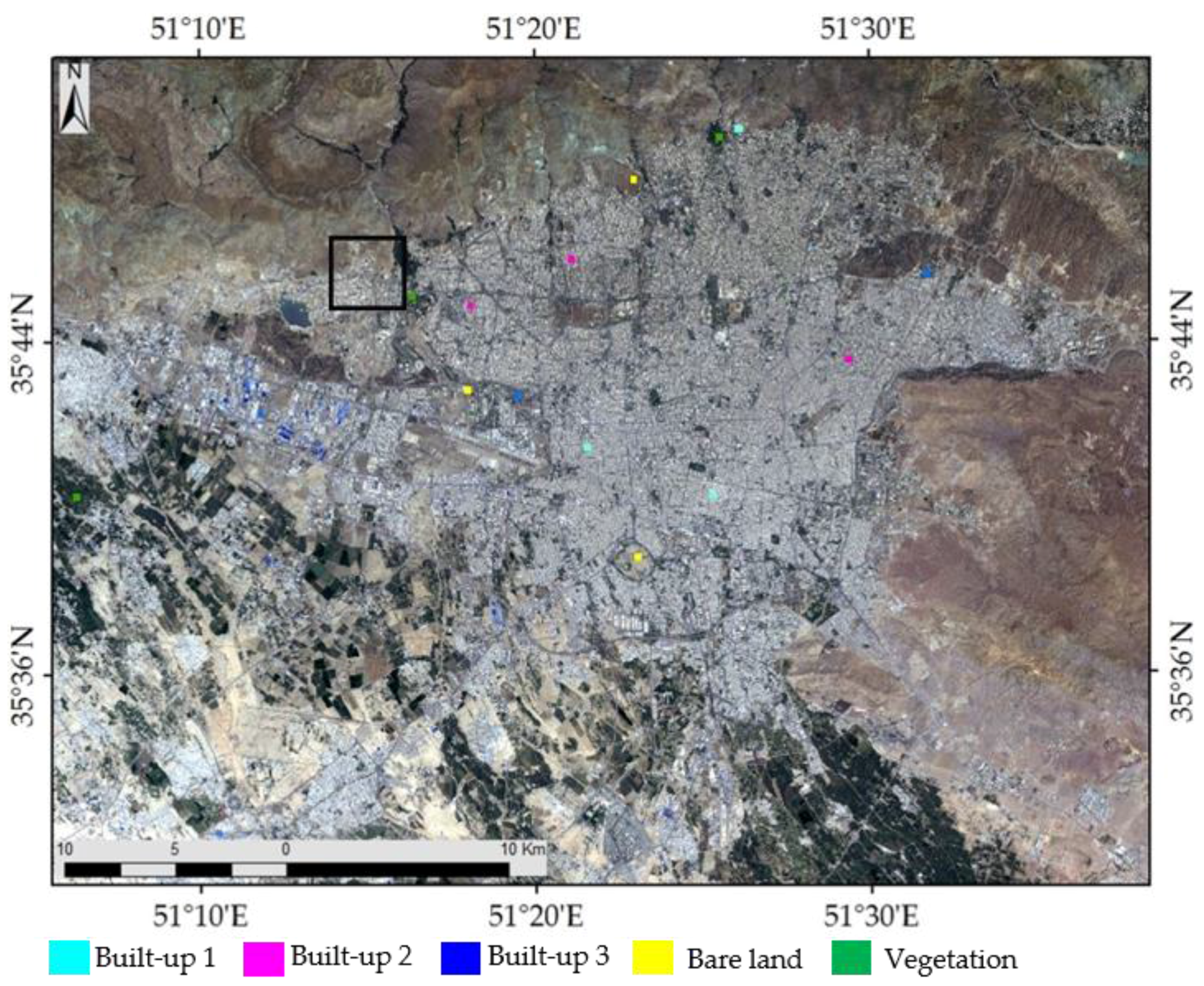
After the inspection of district 22 in Tehran, five land cover classes were defined: bare land, vegetation, built-up 1, built-up 2, and built-up 3. The three different residential types are shown in Figure 3. Built-up 1 is composed of dense residential areas with mostly two-story old buildings and narrow streets and roads. The buildings are approximately 8 × 13 m in size. Built-up 2 is composed of medium density residential areas, including parallel blocks of buildings. The buildings are mostly 12 × 18 m in size. These buildings consist of approximately 4–6 floors. Built-up 3 includes individual building with 4–15 floors. Built-up 3 has wider streets than the other areas and plenty of vegetation surrounding the buildings. The buildings are mostly two different shapes, square with a size of 25 × 25 m or rectangular with a size of approximately 25 × 44 m. For each of these five land cover classes, three training samples were selected. The training samples mainly consist of square shapes of 200 m in length, which are located in different parts of Tehran, as shown in Figure 4.
The classification process was performed using two algorithms: support vector machine (SVM) and maximum likelihood (ML). Both algorithms are derived from statistical theories. These two methods are commonly used in land cover classification studies [37,38,39,40,41]; therefore, we intend to evaluate their performance for SAR data imagery. Supervised classifiers were applied to three sets of data: (1) Landsat 8 multi-spectral image; (2) Backscatter values of dual-polarization ALOS-2 and Sentinel-1 data; and (3) the layer stacking of backscatter values and the first three PCTs from ALOS-2 and Sentinel-1 data.
The maximum likelihood method works based on the assumption that each class is normally distributed. Thus, for each pixel, the probability that it belongs to a specific class is calculated. Then, the pixel is assigned to the class that yields the highest probability as follows [36,42]:
where i is the number of classes, x represents the n-dimensional data (where n is the number of bands), p(ωi) denotes the probability that class ωi occurs in the image and is assumed to be the same for all classes, |Σi| is the determinate of the covariance matrix of the data in class ωi, Σi−1 is its inverse matrix, and mi represents the mean vector.
Support vector machine is a trusted algorithm often used in remote sensing [43,44]. This algorithm was developed by Vanpik [45], and its use has increased for land cover classification in recent years. The SVM separates the pixels of an image using optimal hyperplanes that maximize the margin between the classes [46]. The data points closest to a hyperplane are called support vectors. A nonlinear classification can be performed using kernel functions to the support vectors. In this study, the pairwise strategy is used for multi-class classification. We selected the radial basis function, which is a common kernel type one for the classification and is expressed as follows:
where xi and xj represent the training data and class labels, and g is the gamma term in the kernel function [47,48,49]. Radial basis functions with gamma value of 1.12 and 1.14 were used for SAR and optical image, respectively. The gamma value was calculated by inversing of the number of bands in the input image.
Moreover, the memory usage and the speed of training were not considered for either supervised algorithms in this study because the scope of this research is to evaluate the improvement of the accuracy after introducing the texture feature.
3.4. Accuracy Assessment
The accuracy of the results from the ML and SVM methods was measured by calculating a confusion matrix. The confusion matrix compares the classified land cover with truth data and is a standard method used to evaluate the accuracy of classification in remote sensing [50]. The overall accuracy, producer and user accuracies, and kappa coefficient are calculated from this matrix.
In this research, the confusion matrix was prepared using truth data over the five land cover classes. Based on the comparison of the confusion matrix of the classification results, we evaluated the effect of the supervised classification algorithms and texture measures.
4. Results and Discussion
This study aims to classify the land covers in Tehran city with high accuracy using appropriate datasets and methodologies. A multi-spectral Landsat 8 image and SAR data (ALOS-2 and Sentinel-1) were used to evaluate the performance of the supervised classification algorithms, maximum likelihood and support vector machine. The comparison and evaluation of the results from the optical and SAR sensors are presented in the following.
4.1. Multi-Spectral Optical Image
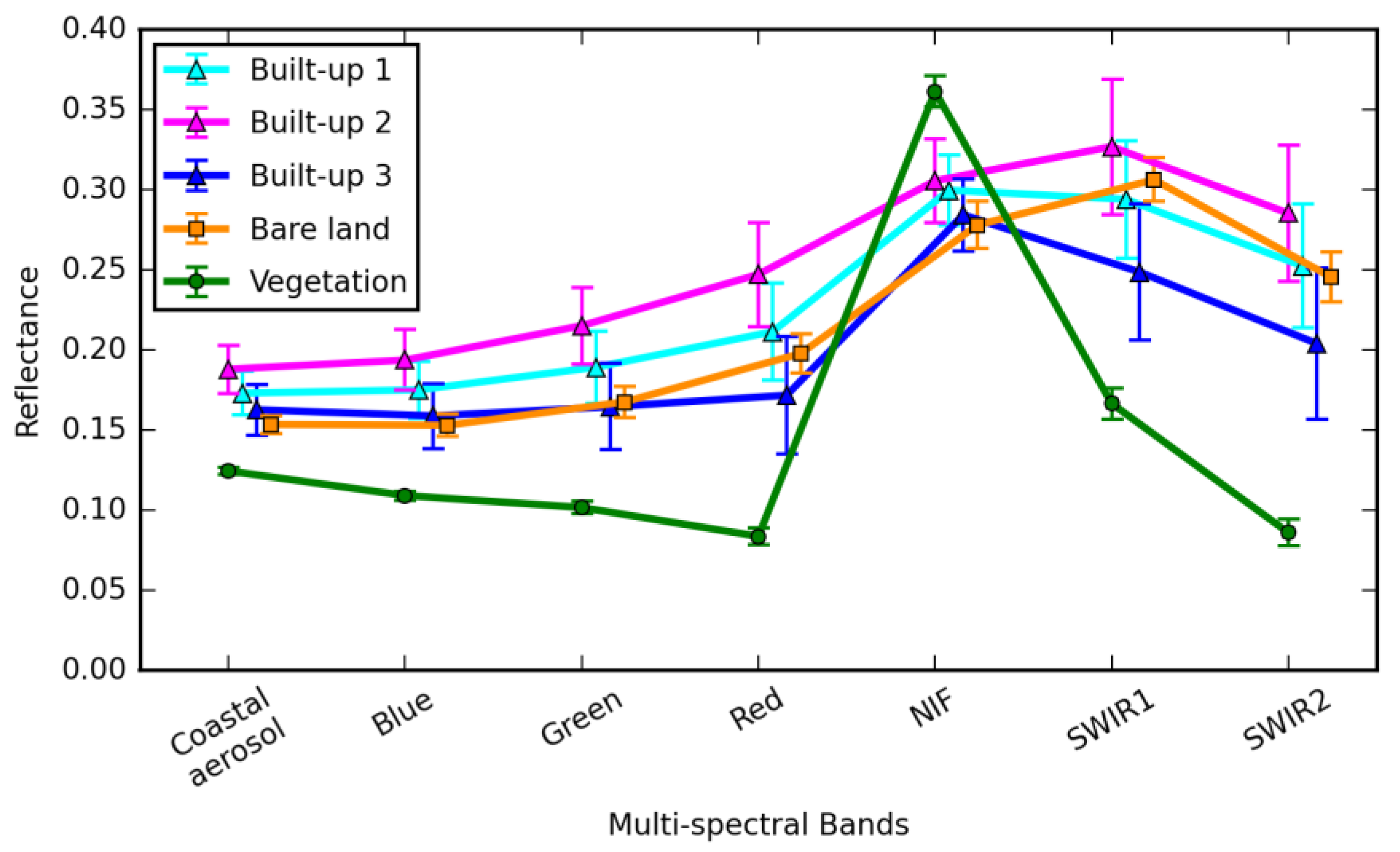
Regarding the aim of this study, we begin by observing the performance of the multi-spectral optical image. First, the spectral signatures of the different land cover samples from the Landsat 8 image (Figure 4) for the built-up 1, built-up 2, built-up 3, bare land, and vegetation classes are shown in Figure 5. The spectral reflectance characteristics of bare lands and built-up features are remarkably similar, while the vegetation signature shows a different pattern. The geography of the study area makes it difficult to differentiate the urban area from the mountainous and desert areas that surround Tehran. ML and SVM classifications were applied to the Landsat 8 image using a total of fifteen training samples from five different land cover types. The results are shown in Figure 6. The ML classification result (Figure 6a) indicates that almost all bare land and mountain areas around Tehran were selected as built-up area (built-up 1). Additionally, the SVM result (Figure 6b) shows that some bare land areas in the southeast and west of Tehran were classified incorrectly as built-up areas (built-up 1 and 2).
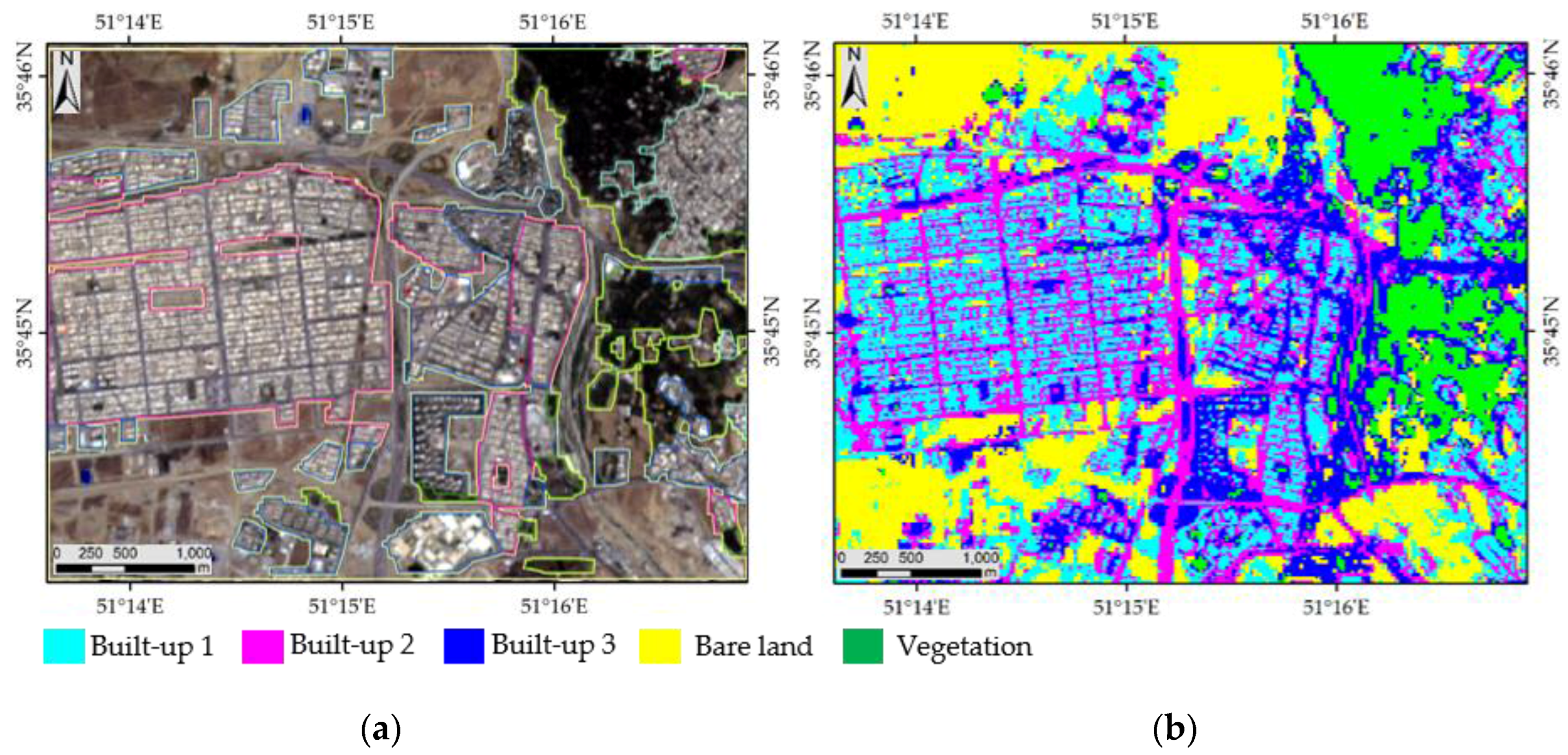
To validate the classification result, we prepared the confusion matrix using the truth data. Figure 7a represents a closer look of the validation area, which is shown by a black frame in Figure 4 and Figure 6b as well. Table 2 illustrates the confusion matrix results from Landsat 8 using SVM and ML classification. The SVM classification gave an overall accuracy and kappa coefficient of 41.1% and 0.26, respectively, while ML gave the values of 35.3% and 0.22. Moreover, the producer and user accuracy are shown in table below. The producer accuracy represents the correctly classified pixels out of the truth pixels of related land cover classes. The user accuracy, illustrates the correctly classified pixels out of the total classified pixels. The SVM algorithm provided higher accuracy than ML. A closer look at the SVM result is shown in Figure 7b. It is observed that some classes were incorrectly classified, such as built-up 2, which was mostly classified as built-up 1. Therefore, the Landsat 8 image does not seem appropriate for classifying the land cover of the study area, Tehran city.
4.2. SAR Data
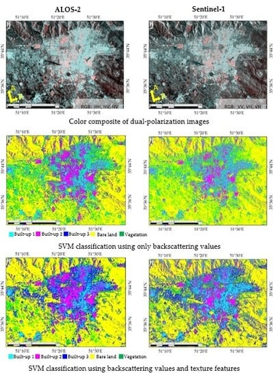
Considering the limitation of the Landsat 8 image in land cover classification and detection of various built-up classes and bare land in the study area, ALOS-2 and Sentinel-1 images with the capability of obtaining ground surface information based on the backscatter coefficient were selected to overcome this issue. Figure 8 represents the color composites of the dual-polarization intensity images from the ALOS-2 and Sentinel-1 data. The cyan and red colors indicate different orientation and geometrical positions of the residential areas in Tehran.
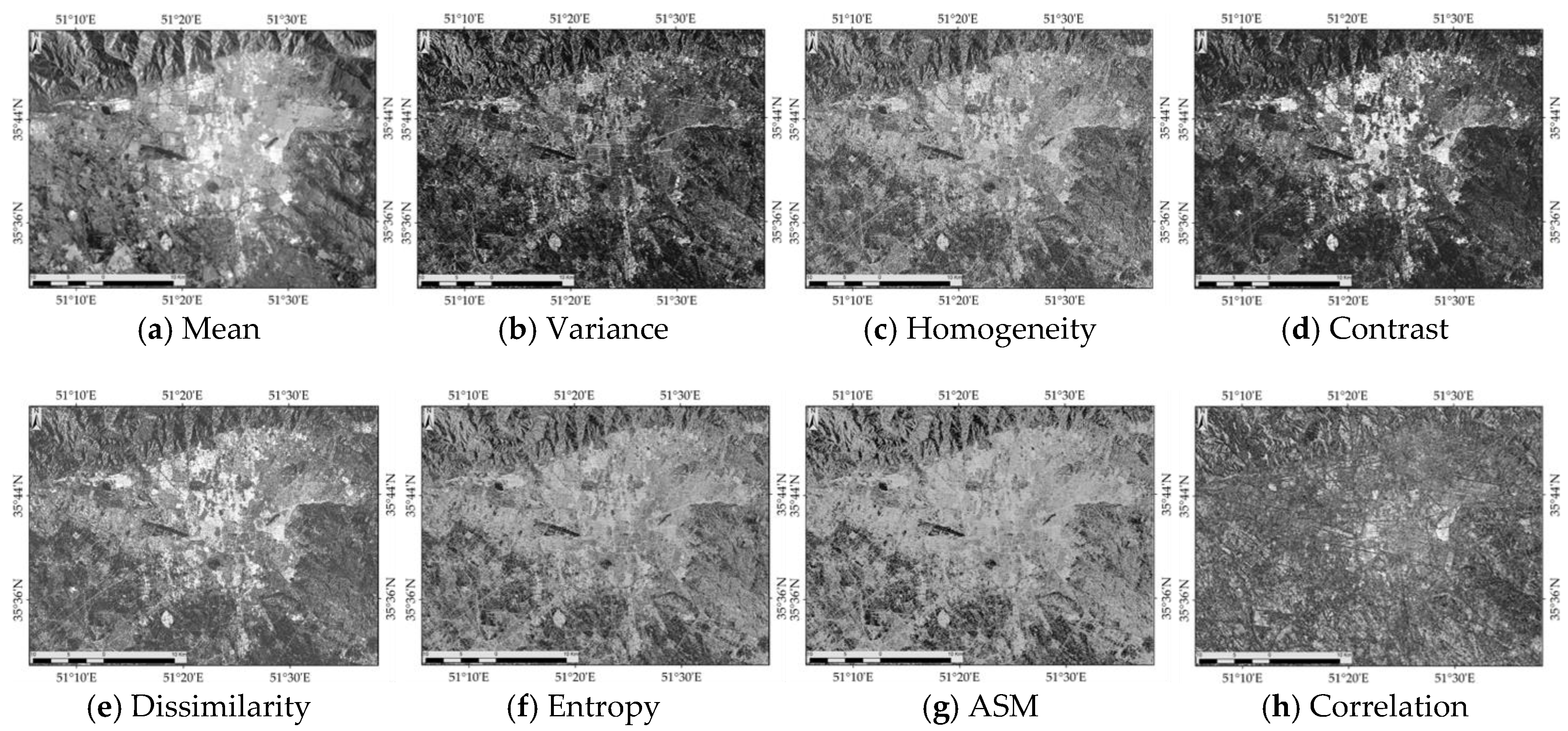
To increase the accuracy in the supervised classification from SAR data, texture analysis (GLCM) was applied to the dual-polarization images. Figure 9 depicts the texture features obtained from ALOS-2 HH polarization. Texture analysis was applied to each backscatter value of HH, HV, VV, and VH. Thus, for each polarized image, eight texture measures were obtained: mean, contrast, ASM, correlation, homogeneity, variance, entropy, and dissimilarity. Then, the PCA was applied to reduce the number of textures measured.
In order to select the appropriate number of principal components for texture measures (PCT) to perform the classification, we examined the region shown as a yellow frame in Figure 8 using the HH and HV polarizations of ALOS-2. The SVM classification was carried out for two datasets. In the first dataset, the two backscatter values (HH and HV) and all their PCTs (18 layers in total) were used. In the second dataset, the two backscatter values and their first three PCTs (eight layers in total) were used. In both datasets the PCT was calculated from texture features obtained using a window size of 13 × 13. The first three components contain almost 99 percent of the variation of the input elements. Table 3 shows the overall accuracy and the kappa coefficient obtained from the classification of the two datasets. A comparison shows a difference of only 1.26% for the overall accuracy and a difference of 0.02 for the kappa coefficient. Although the dataset with all the PCTs gained higher accuracy, the required time was significantly larger than that of the second dataset. Therefore, in this study, only the first three principal components were used.
Figure 10 illustrates the first three PCTs of the HH polarization. The classifications using ML and SVM were performed using the same fifteen training samples shown in Figure 4. As mentioned before, the performance of both ML and SVM are compared to the truth data to observe which method produces the highest accuracy.
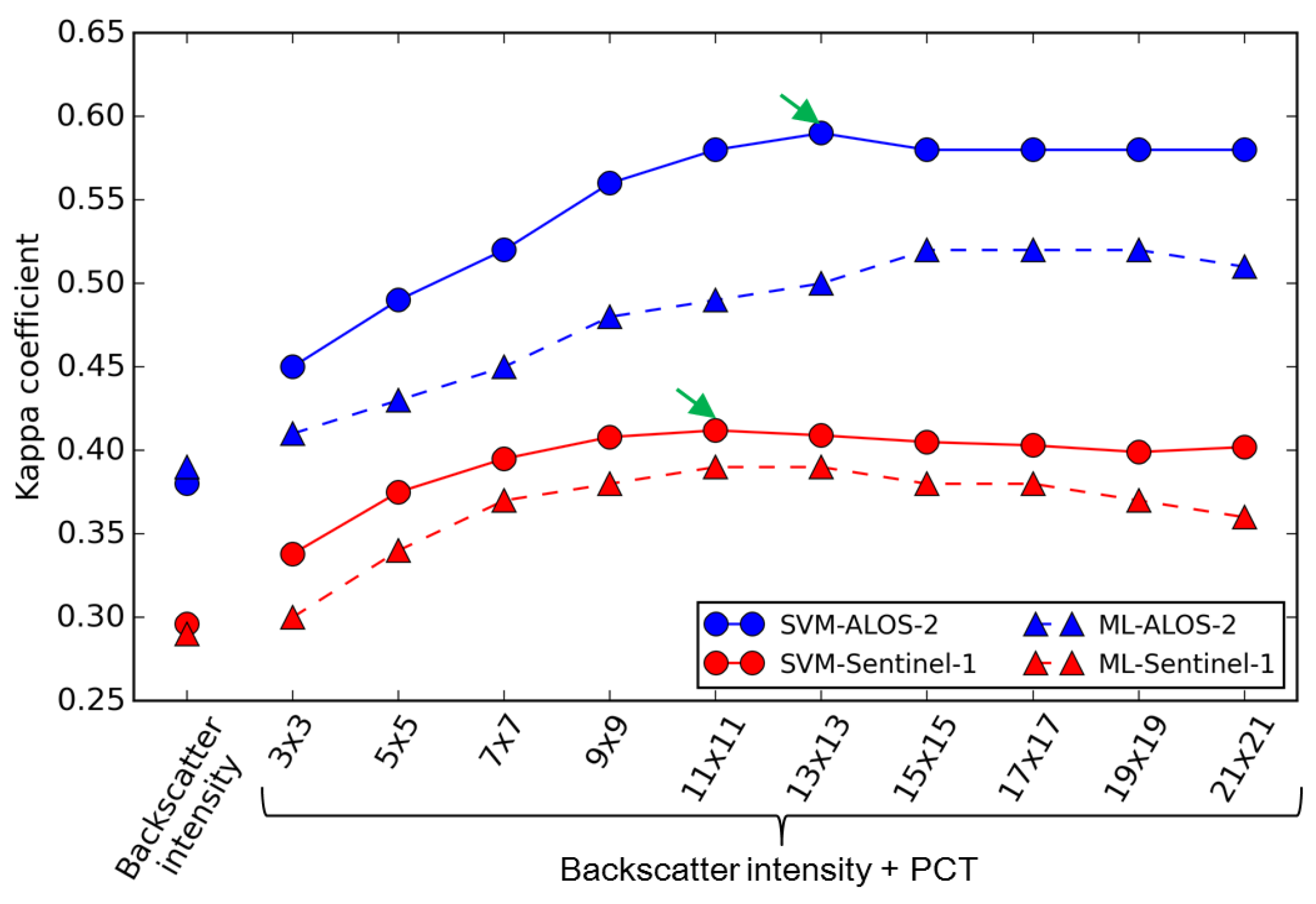
The window size is an important parameter for the texture measures. In this study, window sizes ranging from 3 × 3 to 21 × 21 were all evaluated to estimate the most suitable window size. Figure 11 shows the kappa coefficients for the classification using only the backscatter values of ALOS-2 (HH, HV) and Sentinel-1 (VV, VH), and those by the layer stacking of the backscatter values and their PCTs results for different window sizes. The numbers of pixels in each land cover class in the truth data are not equal, thus the kappa coefficient is plotted in Figure 11. The solid lines represent the results from SVM classification and the dashed lines those from ML classification, both for ALOS-2 and Sentinel-1. The graph shows an increase of the kappa coefficient by introducing the texture measures for the classification. The performance of SVM is better than that of ML classification. For the ALOS-2 satellite, the difference between the both methods increases significantly when the texture window size increases. The highest kappa coefficient was observed in the classification for ALOS-2 with window size 13 by SVM as shown by green arrow in the graph. The highest kappa coefficient of Sentinel-1 classification results was obtained from SVM in window size 11 × 11. Moreover, ALOS-2 provided better performance than Sentinel-1.
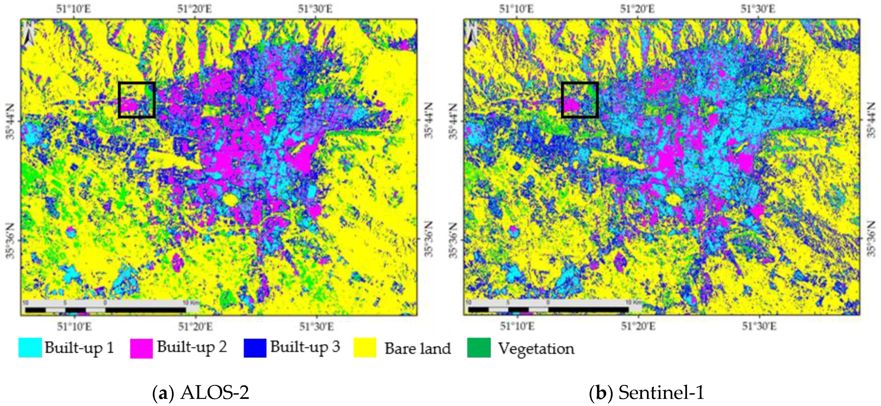
Figure 12 illustrates the SVM classification of Tehran using the layer stacking of backscatter values and their PCTs for the both ALOS-2 and Sentinel-1 satellites. The PCT was calculated using a window sizes of 13 × 13 and 11 × 11 for the ALOS-2 and Sentinel-1, respectively.
Herein, further evaluation is performed only for the datasets that produced the highest kappa coefficient. Thus, for the sake of brevity, the classification result from the ALOS-2 backscatter values and their first three PCTs using a window size of 13 × 13 is referred as ALOS-2-PCT. Similarly, the classification result from the Sentinel-1 backscatter values and their first three PCTs using a window size of 11 × 11 is referred as Sentinel-1-PCT. Table 4, Table 5 and Table 6 illustrate the confusion matrix for the Landsat-8 image, ALOS-2 (backscatter values only), and ALOS-2-PCT, respectively. Table 7 and Table 8 represent the confusion matrix for the Sentinel-1, and the Sentinel-1 PCT, respectively. The tables show a remarkable improvement in both overall accuracy and kappa coefficient for the datasets that include texture measures over the datasets of only backscattering values and Landsat 8. The Landsat 8 produced an overall accuracy and kappa coefficient of 41.1% and 0.25, respectively. Table 5 and Table 6 depict that the overall accuracy and kappa coefficient of the ALOS-2-PCT is greater than the ALOS-2. The overall accuracy increased from 53.0% to 69.7% and the kappa coefficient from 0.38 to 0.58 when the texture measures of window size 13 × 13 were included. Moreover, the Sentinel-1 PCT shows higher overall accuracy and kappa coefficient than the Sentinel-1. Table 7 and Table 8 show an increase from 45.7% to 54.2% for the overall accuracy and an increment from 0.29 to 0.41 for the kappa coefficient when the textures of window size 11 × 11 were included.
The confusion matrix includes the producer and user accuracies as well. The diagonal elements in these tables depict the correctly classified pixels in each land cover class. The comparison shows that the highest producer accuracy was obtained when the texture features were included (Table 6 and Table 8). It can be observed from Table 4 and Table 5 that, although the producer accuracy increased for the bare land, built-up 1 and built-up 2 classes when the SAR backscatter values in classification is used instead of the Landsat 8, the producer accuracy decreased for the built-up 3 and vegetation classes from 27.1% and 63.8% to 15.6% and 59.6%. However, when texture features are included, an improvement is observed for all the land cover classes. Thus, in our study area, classification of land cover using SAR backscatter and texture feature is superior in terms of accuracy than classification from the Landsat 8 and SAR backscatter only. Furthermore, the user accuracy increased in all classes except vegetation for the ALOS-2-PCT. In case of the Sentinel-1, the user accuracy for the dataset including the texture measures improved in all the classes comparing with the dataset of backscattering values only and there was no improvement for the bare land and vegetation comparing with the Landsat 8 dataset.
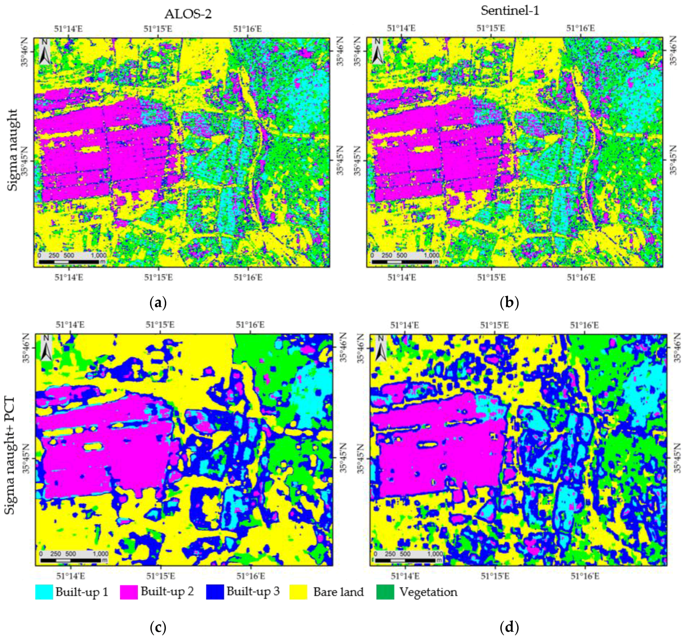
Figure 13 shows a closer look of SVM classification for the ALOS-2, Sentinel-1, ALOS-2-PCT, and Sentinel-1-PCT. The location of the area is shown in Figure 12. The improvement in the accuracy mentioned before can be appreciated visually in this figure. The most remarkable observation is that when using texture measures of the SAR data for classification, the producer accuracy improved significantly, therefore, the amount of noise and misclassified pixels for all classes decreased and the classes become more uniform comparing to that using only SAR backscatter values or optical data.
5. Conclusions
In this study, the GLCM texture measures were applied to improve the supervised classification of SAR intensity images for urban areas. For this purpose, Tehran was selected as the study area because of its rapid expansion, which has resulted in land cover changes and the appearance of new urban regions. Due to the similarity of the spectral signatures of soil and roof material in built-up regions, classification from multi-spectral optical images seems very difficult. Alternatively, SAR images may be a better option because the backscattering depends on the geometrical features of the objects within the recorded area. Dual-polarized data from L-band ALOS-2 (HH, HV) and C-band Sentinel-1 (VV, VH) were employed. In addition, the texture properties were calculated by applying a gray-level co-occurrence matrix (GLCM). Thus, eight texture features were obtained for each intensity element. Furthermore, a principal component analysis was applied to each set of texture measures, and the first three components were selected based on the greatest covariance. Then, maximum likelihood and support vector machine algorithms were used for the three datasets: optical images and the SAR intensity data without and with texture measures. The results of the supervised classification were compared with the truth data obtained by visual inspection of the Landsat 8 image.
The supervised classification results with texture measures were found to be superior to the results without texture in two main aspects: the highest accuracy and least noise. The support vector machine for both the optical and SAR sensors produced a higher accuracy than the maximum likelihood. Moreover, the classification of ALOS-2 with the SVM methodology using a window size of 13 × 13 obtained the highest overall accuracy. Besides, Sentinel-1 gained the best accuracy in window size 11 × 11 with SVM classification. Although the intermediate window sizes of 13 × 13 and 11 × 11 worked well in this study area, the best window size could change based on the different study areas and truth data using for assessing the accuracy.
Acknowledgments
The ALOS-2 PALSAR-2 data used in this study are owned by the Japan Aerospace Exploration Agency (JAXA) and were provided through the JAXA’s ALOS-2 research program (RA4, PI No. 1503). The Pleiades images are owned by Airbus Defense and Space and licensed to Chiba University.
Author Contributions
This research was conducted by Homa Zakeri for her Doctoral studies under the supervision of Fumio Yamazaki and guidance of Wen Liu. All authors read and reviewed the article.
Conflicts of Interest
The authors declare no conflict of interest.
References
- Bhatta, B. Advanced in Geographic Information Science: Analysis of Urban Growth and Sprawl from Remote Sensing Data; Springer: Heidelberg, Germany, 2010; pp. 1–167. [Google Scholar]
- Brando, V.E.; Dekker, A.G. Satellite hyperspectral remote sensing for estimating estuarine and coastal water quality. IEEE Trans. Geosci. Remote Sens. 2003, 41, 1378–1387. [Google Scholar] [CrossRef]
- Molch, K. Radar Earth Observation Imagery for Urban Area Characterisation; JRC Scientific and Technical Reports; European Commission: Luxembourg, 2009; pp. 1–19. [Google Scholar]
- Turner, B.L.; Lambin, E.F.; Reenberg, A. The emergence of land change science for global environmental change and sustainability. Proc. Natl. Acad. Sci. USA 2007, 104, 20666–20671. [Google Scholar] [CrossRef] [PubMed]
- Rathje, E.; Adams, B.J. The Role of Remote Sensing in Earthquake Science and Engineering: Opportunities and Challenges. Earthq. Spectra 2008, 24, 471–492. [Google Scholar] [CrossRef]
- Yamazaki, F.; Inoue, H.; Liu, W. Characteristics of SAR backscattering intensity and its application to earthquake damage detection. In Proceedings of the 6th Conference on Computational Stochastic Mechanics, Rodhes, Greece, 13–16 June 2010; pp. 602–606. [Google Scholar]
- Gong, P.; Wang, J.; Yu, L.; Zhao, Y.; Zhao, Y.; Liang, L.; Niu, Z.; Huang, X.; Fu, H.; Liu, S.; et al. Finer resolution observation and monitoring of global land cover: First mapping results with Landsat TM and ETM+ data. Int. J. Remote Sens. 2012, 34, 2607–2654. [Google Scholar] [CrossRef]
- Liu, W.; Yamazaki, F.; Goken, H.; Koshimura, S. Extraction of Tsunami-Flooded Areas and Damaged Buildings in the 2011 Tohoku-Oki Earthquake from TerraSAR-X Intensity Images. Earthq. Spectra 2013, 29 (Suppl. 1), S183–S200. [Google Scholar] [CrossRef]
- Yamazaki, F.; Liu, W. Urban change monitoring: Multi-temporal SAR images. In Encyclopedia of Earthquake Engineering; Beer, M., Kougioumtzoglou, I., Au, S., Eds.; Springer: Berlin/Heidelberg, Germany, 2015; pp. 3847–3859. [Google Scholar]
- Guan, D.; Li, H.; Inohae, T.; Su, W.; Nagaie, T.; Hokao, K. Modeling urban land use change by the integration of cellular automaton and Markov model. Ecol. Model. 2011, 222, 3761–3772. [Google Scholar] [CrossRef]
- Alqurashi, A.F.; Kumar, L.; Sinha, P. Urban Land Cover Change Modelling Using Time-Series Satellite Images: A Case Study of Urban Growth in Five Cities of Saudi Arabia. Remote Sens. 2016, 8, 838. [Google Scholar] [CrossRef]
- Zhang, J.; Li, P.; Wang, J. Urban built-Up area extraction from landsat TM/ETM+ images using spectral information and multivariate texture. Remote Sens. 2014, 6, 7339–7359. [Google Scholar] [CrossRef]
- Zhang, Y. Optimisation of building detection in satellite images by combining multispectral classification and texture filtering. Photogramm. Remote Sens. 1999, 54, 50–60. [Google Scholar] [CrossRef]
- Colaninno, N.; Roca, J.; Burns, M.; Alhaddad, B.; Patterns, U.; Management, A. Defining densities for urban residential texture, through land use classification, from landsat TM imagery: Case Study of Spanish Mediterranean Coast. In Proceedings of the XXII Congress of the ISPRS Congress, Melbourne, Australia, 25 August–1 September 2012; pp. 179–184. [Google Scholar]
- Henderson, F.M.; Lewis, A.J. Introduction. In Principles and Applications of Imaging Radar, 3rd ed.; Manual of Remote Sensing; John Wiley & Sons Inc.: New York, NY, USA, 1998; pp. 1–6. [Google Scholar]
- Lillesand, T.M.; Kiefer, R.W.; Chipman, J.W. Remote Sensing and Image Interpretation, 5th ed.; John Wiley & Sons Inc.: New York, NY, USA, 2004; pp. 638–713. [Google Scholar]
- Rogan, J.; Chen, D. M. Remote sensing technology for mapping and monitoring Land-cover and land-use change. Prog. Plan. 2004, 61, 301–325. [Google Scholar] [CrossRef]
- Lee, J.S.; Grünes, M.R.; Ainsworth, T.L.; Du, L.J.; Schuler, D.L.; Cloude, S.R. Unsupervised classification using polarimetric decomposition and the complex wishart classifier. IEEE Trans. Geosci. Remote Sens. 1999, 37 Pt 1, 2249–2258. [Google Scholar]
- Hoekman, D.H. A new polarimetric classification approach evaluated for agricultural crops. Eur. Space Agency 2003, 41, 71–79. [Google Scholar] [CrossRef]
- Dell’Acqua, F.; Gamba, P. Texture-based characterization of urban environmental on satellite SAR images. IEEE Trans. Geosci. Remote Sens. 2003, 41, 153–159. [Google Scholar] [CrossRef]
- Matsuoka, M.; Yamazaki, F. Use of satellite SAR intensity imagery for detecting building areas damaged due to earthquakes. Earthq. Spectra 2004, 20, 975–994. [Google Scholar] [CrossRef]
- Haralick, R.; Shanmugan, K.; Dinstein, I. Textural features for image classification. IEEE Trans. SMC 1973, 3, 610–621. [Google Scholar] [CrossRef]
- Augusteijn, M.F.; Clemens, L.E.; Shaw, K.A. Performance evaluation of texture measures for ground cover identification in satellite images by means of a neural network classifier. IEEE Trans. Geosci. Remote Sens. 1995, 33, 616–626. [Google Scholar] [CrossRef]
- Shaban, M.A.; Dikshit, O. Improvement of classification in urban areas by the use of textural features: The case study of Lucknow City, Uttar Pradesh. Int. J. Remote Sens. 2010, 22, 565–593. [Google Scholar] [CrossRef]
- Lu, D.; Batistella, M.; Moran, E. Integration of Landsat TM and SPOT HRG Images for Vegetation Change Detection in the Brazilian Amazon. Photogramm. Eng. Remote Sens. 2008, 74, 421–430. [Google Scholar] [CrossRef]
- Clausi, D.A.; Yu, B. Comparing co-occurrence probabilities and Markov random fields for texture analysis of SAR Sea ice imagery. IEEE Trans. Geosci. Remote Sens. 2004, 42, 215–228. [Google Scholar] [CrossRef]
- Kandaswamy, U.; Adjeroh, D.A.; Lee, M.C. Efficient Texture Analysis of SAR Imagery. IEEE Trans. Geosci. Remote Sens. 2005, 43, 2075–2083. [Google Scholar] [CrossRef]
- Atlas of Tehran Metropoli. Available online: http://atlas.tehran.ir/Default.aspx?tabid=227 (accessed on 11 February 2017).
- Madanipour, A. Urban planning and development in Tehran. Cities 2006, 23, 433–438. [Google Scholar] [CrossRef]
- District 22 of Tehran Municipality. Available online: http://region22.tehran.ir/ (accessed on 11 February 2017).
- Advanced Land Observing Satellite DAICHI-2. DAICHI. Available online: http://www.eorc.jaxa.jp/ALOS/en/top/about_top.htm (accessed on 11 February 2017).
- Sentinel Online. Available online: https://sentinel.esa.int/web/sentinel/missions/sentinel-1/instrument-payload (accessed on 11 February 2017).
- Lee, J.S.; Grunes, M.R.; de Grandi, G. Polarimetric SAR Speckle Filtering and Its Implication for Classification. IEEE Trans. Geosci. Remote Sens. 1999, 37, 2363–2373. [Google Scholar]
- Ulaby, F.T.; Moore, R.K.; Fung, A.K. Microwave Remote Sensing: Active and Passive, Radar Remote Sensing and Surface Scattering and Emission Theory, 82nd ed.; Addison Wesley: Boston, MA, USA, 1982; Volume 2, pp. 1–624. [Google Scholar]
- Anyamba, A.; Eastman, J.R. Interannual variability of NDVI over Africa and its relation to El Nino/Southern Oscillation. Int. J. Remote Sens. 1996, 17, 2533–2548. [Google Scholar] [CrossRef]
- Richards, J.A. Remote Sensing Digital Image Analysis, 5th ed.; Springer: Berlin/Heidelberg, Germany, 2013; pp. 192–195. [Google Scholar]
- Skriver, H. Crop classification by multitemporal C- and L-band single- and dual-polarization and fully polarimetric SAR. IEEE Trans. Geosci. Remote Sens. 2012, 50, 2138–2149. [Google Scholar] [CrossRef]
- Lee, J.S.; Grunes, M.R.; Pottier, E. Quantitative comparison of classification capability: Fully polarimetric versus dual and single-polarization SAR. IEEE Trans. Geosci. Remote Sens. 2001, 39, 2343–2351. [Google Scholar]
- Waske, B.; Benediktsson, J.A. Fusion of support vector machines for classification of multisensor data. IEEE Trans. Geosci. Remote Sens. 2007, 45, 3858–3866. [Google Scholar] [CrossRef]
- Lardeux, C.; Frison, P.L.; Tison, C.; Souyris, J.C.; Stoll, B.; Fruneau, B.; Rudant, J.P. Support vector machine for multifrequency SAR polarimetric data classification. IEEE Trans. Geosci. Remote Sens. 2009, 47, 4143–4152. [Google Scholar] [CrossRef]
- Mountrakis, G.; Im, J.; Ogole, C. Support vector machines in remote sensing: A review. Photogramm. Remote Sens. 2011, 66, 247–259. [Google Scholar] [CrossRef]
- Strahler, H. The use of prior probabilities in MaximumLikelihood Classification of remotely sensed data. Remote Sens. Environ. 1980, 10, 135–163. [Google Scholar]
- Huang, C.; DAVIS, L.S.; Townshen, J.R.G. An assessment of support vector machines for land cover classification. Int. J. Remote Sens. 2002, 23, 725–749. [Google Scholar] [CrossRef]
- Wieland, M.; Liu, W.; Yamazaki, F. Learning Change from Synthetic Aperture Radar Images: Performance Evaluation of a Support Vector Machine to Detect Earthquake and Tsunami-Induced Changes. Remote Sens. 2016, 8, 792. [Google Scholar] [CrossRef]
- Vapnik, V. The Nature of Statistical Learning Theory, 2nd ed.; Springer: New York, NY, USA, 2000; pp. 1–340. [Google Scholar]
- Pal, M.; Mather, P.M. Support vector machines for classification in remote sensing. Int. J. Remote Sens. 2005, 26, 1007–1011. [Google Scholar] [CrossRef]
- Chang, C.C.; Lin, C.J. LIBSVM: A library for support vector machines. J. ACM Trans. Intell. Syst. Technol. 2001, 2, 1–23. [Google Scholar] [CrossRef]
- Hsu, C.-W.; Chang, C.-C.; Lin, C.-J. A Practical Guide to Support Vector Classification; Technical Report; Department of Computer Science, National Taiwan University: Taipei, Taiwan, 2010; pp. 1–16. [Google Scholar]
- Wu, T.F.; Lin, C.J.; Weng, R.C. Probability estimates for multi-class classification by pairwise coupling. J. Mach. Learn. Res. 2004, 5, 975–1005. [Google Scholar]
- Paneque-Gálvez, J.; Mas, J.F.; Moré, G.; Cristóbal, J.; Orta-Martínez, M.; Luz, A.C.; Reyes-García, V. Enhanced land use/cover classification of heterogeneous tropical landscapes using support vector machines and textural homogeneity. Int. J. Appl. Earth Obs. Geoinf. 2013, 23, 372–383. [Google Scholar] [CrossRef]
Figure 1.
Location of Tehran and coverage of the satellite images used in this study, including Sentinel-1 (blue frame) acquired on 26 October 2015, ALOS-2 (red frame) acquired on 14 October 2015 and Landsat 8 (green frame) acquired on 7 May 2015.
Figure 1.
Location of Tehran and coverage of the satellite images used in this study, including Sentinel-1 (blue frame) acquired on 26 October 2015, ALOS-2 (red frame) acquired on 14 October 2015 and Landsat 8 (green frame) acquired on 7 May 2015.

Figure 2.
Flowchart of land cover classification using the multi-spectral optical image and two synthetic aperture radar (SAR) datasets. GLCM: gray-level co-occurrence matrix; SVM: support vector machine; ML: Maximum Likelihood; PCT: principal components of the textures.
Figure 2.
Flowchart of land cover classification using the multi-spectral optical image and two synthetic aperture radar (SAR) datasets. GLCM: gray-level co-occurrence matrix; SVM: support vector machine; ML: Maximum Likelihood; PCT: principal components of the textures.
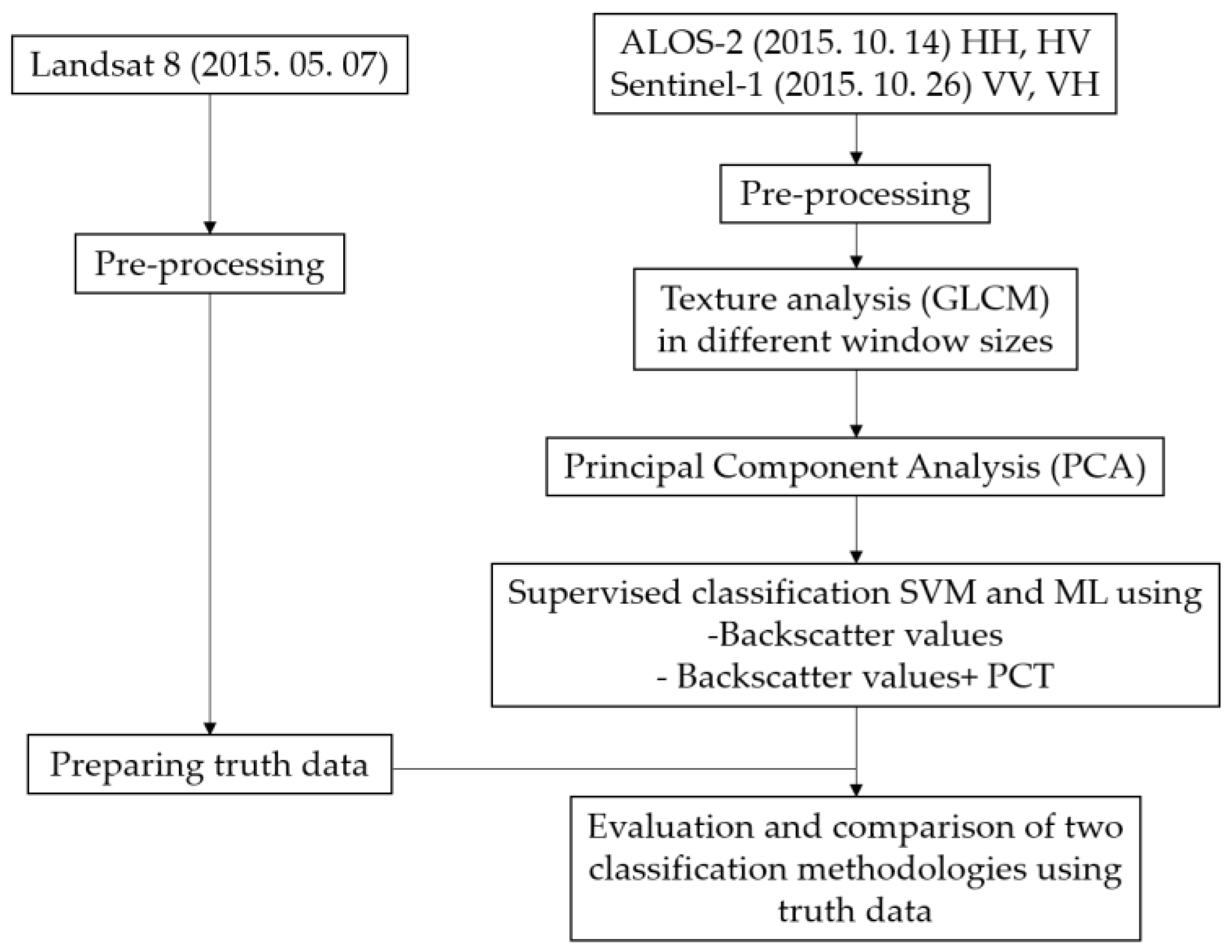
Figure 3.
Three different residential types (a–c) extracted from Google Earth images of Tehran city.
Figure 3.
Three different residential types (a–c) extracted from Google Earth images of Tehran city.
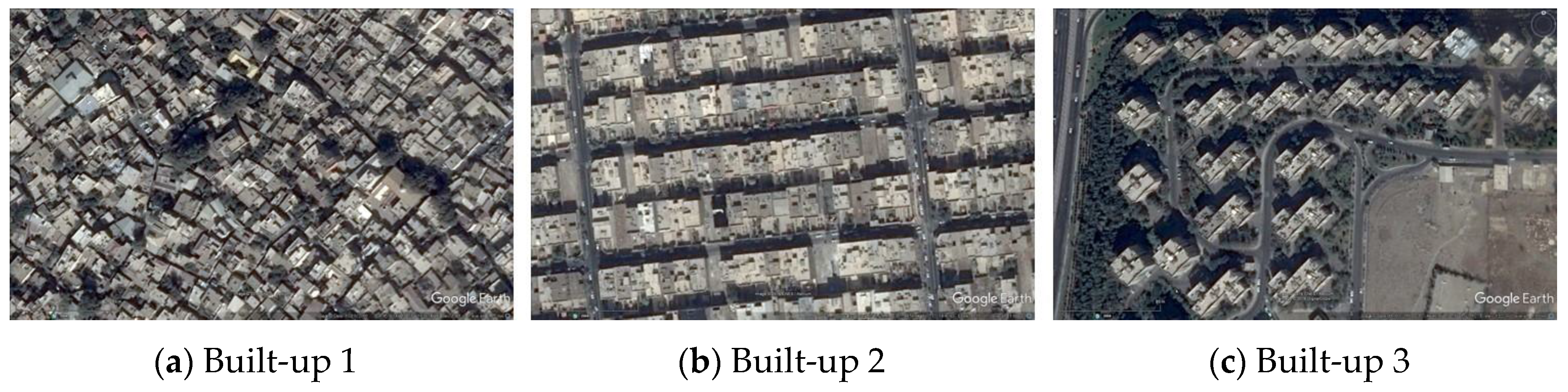
Figure 4.
The three training samples selected for each land cover class from the Landsat 8 image used for supervised classification. The black frame shows the area used for assessing the accuracy.
Figure 4.
The three training samples selected for each land cover class from the Landsat 8 image used for supervised classification. The black frame shows the area used for assessing the accuracy.

Figure 5.
Spectral signatures of the five land covers obtained from the Landsat 8 image.

Figure 6.
The ML (a) and SVM (b) classification results of Landsat 8 image, where the black frame shows the location of the validation area.
Figure 6.
The ML (a) and SVM (b) classification results of Landsat 8 image, where the black frame shows the location of the validation area.
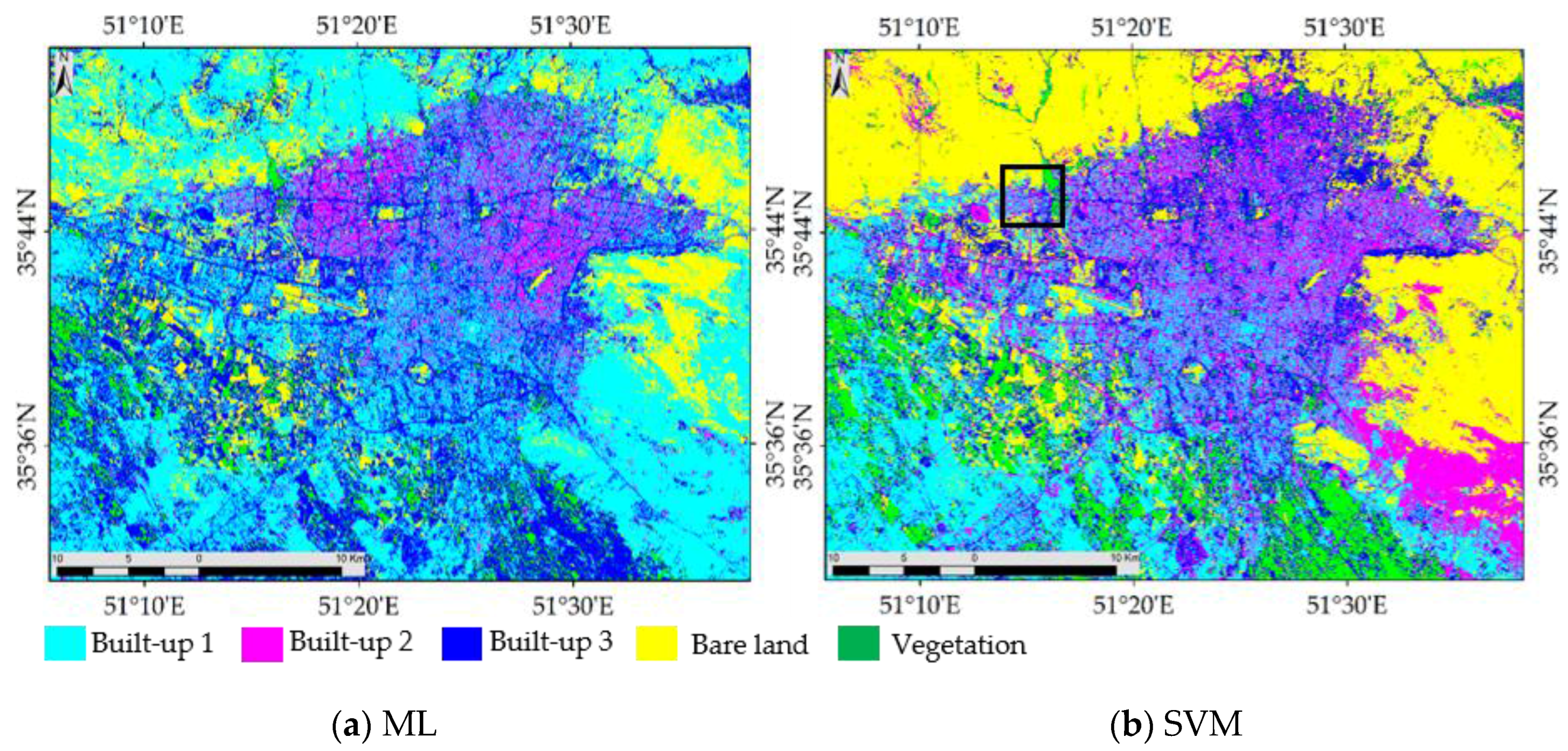
Figure 7.
Validation area containing the truth data for the five classes (a); and the result of the SVM classification from Landsat 8 image (b).
Figure 7.
Validation area containing the truth data for the five classes (a); and the result of the SVM classification from Landsat 8 image (b).

Figure 8.
Color composite of dual-polarization images from the ALOS-2 image (a) and the Sentinel-1 image (b), the yellow frame shows the location of region chosen for evaluating the components of principal component analysis (PCA) and the location of validation area.
Figure 8.
Color composite of dual-polarization images from the ALOS-2 image (a) and the Sentinel-1 image (b), the yellow frame shows the location of region chosen for evaluating the components of principal component analysis (PCA) and the location of validation area.
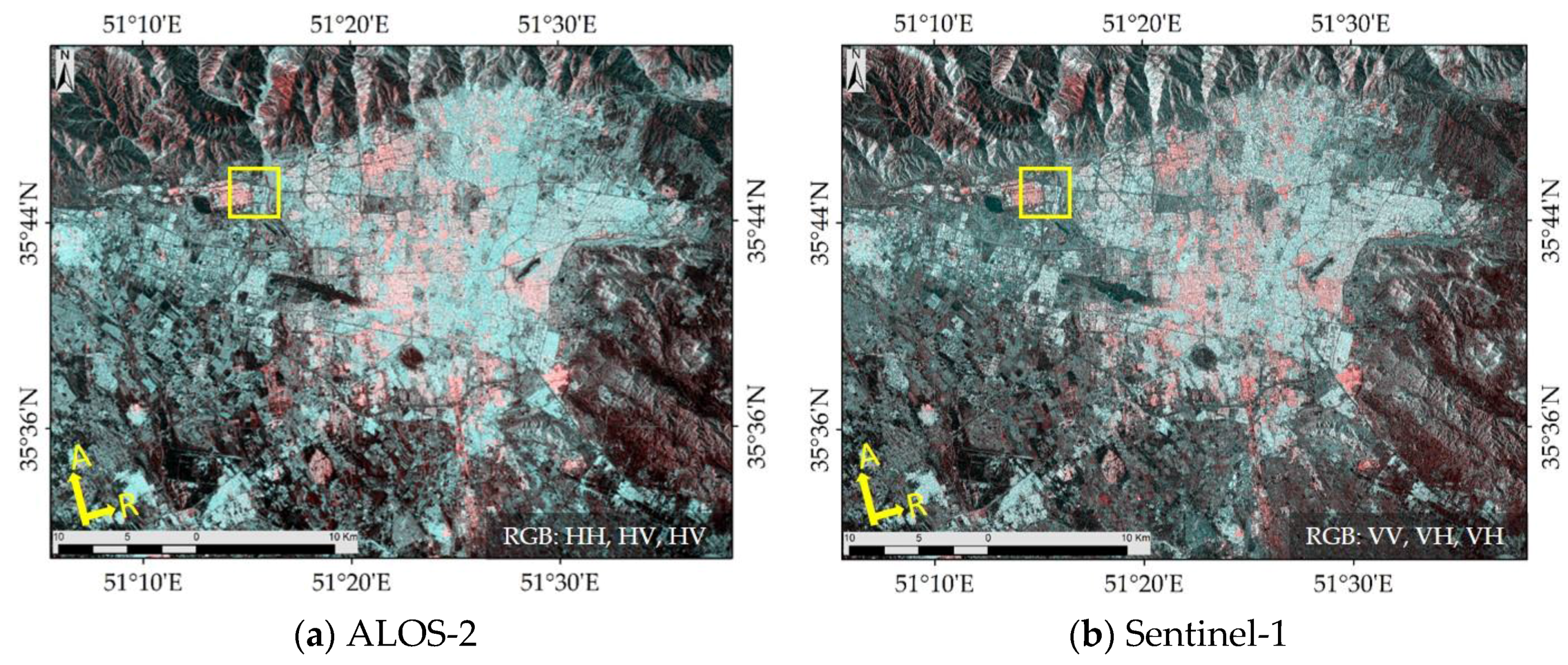
Figure 9.
Eight texture features (a–h) obtained from the ALOS-2 HH polarization with a window size of 13 × 13, angle of 0°, and displacement of 1 pixel.
Figure 9.
Eight texture features (a–h) obtained from the ALOS-2 HH polarization with a window size of 13 × 13, angle of 0°, and displacement of 1 pixel.

Figure 10.
The first three principal components (a–c) prepared from the eight texture features of the ALOS-2 HH polarization.
Figure 10.
The first three principal components (a–c) prepared from the eight texture features of the ALOS-2 HH polarization.
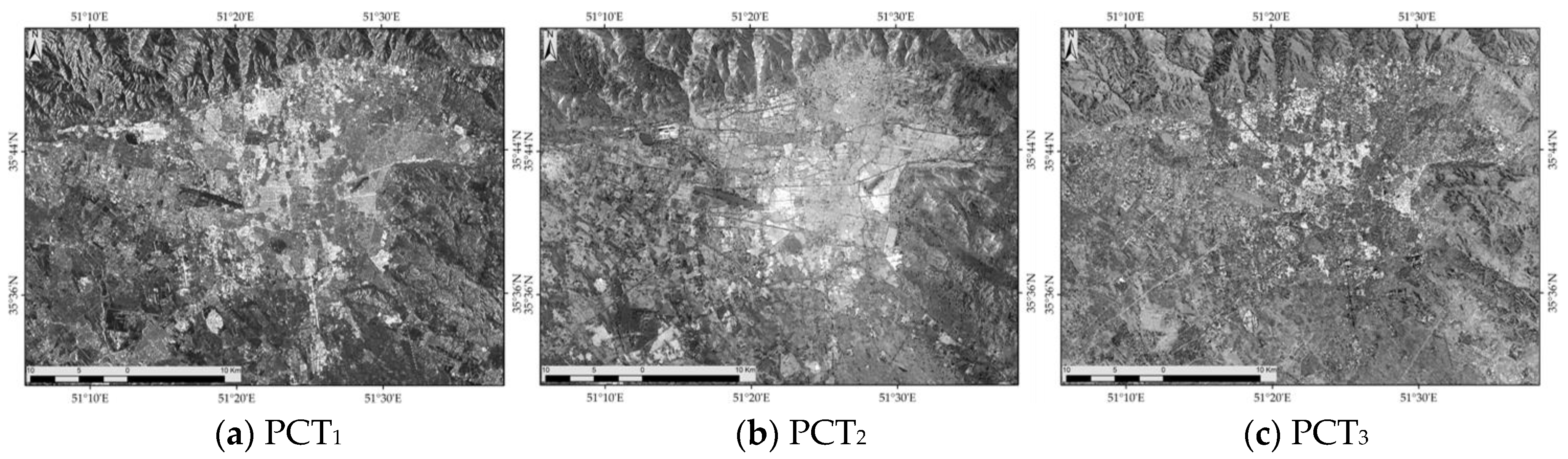
Figure 11.
Kappa coefficient calculated from SVM and ML classification methods using only the backscatter of ALOS-2 and Sentinel-1 and those by the layer stacking of the backscatter values and their PCTs for window sizes ranging from 3 × 3 to 21 × 21. Green arrows show the highest Kappa coefficient.

Figure 12.
SVM classification results of backscatter values and their PCTs from the ALOS-2 image using a window size of 13 × 13 (a) and the Sentinel-1 image using a window size of 11 × 11 (b). The black frame represents the location of Figure 13.
Figure 12.
SVM classification results of backscatter values and their PCTs from the ALOS-2 image using a window size of 13 × 13 (a) and the Sentinel-1 image using a window size of 11 × 11 (b). The black frame represents the location of Figure 13.

Figure 13.
A close-up of the SVM classification results from the ALOS-2 (a); Sentinel-1 (b); ALOS-2 PCT (c); and Sentinel-1 PCT (d).
Figure 13.
A close-up of the SVM classification results from the ALOS-2 (a); Sentinel-1 (b); ALOS-2 PCT (c); and Sentinel-1 PCT (d).

Table 1.
The change of population in Tehran [28].
Table 1.
The change of population in Tehran [28].
| Year | 1986 | 1991 | 1996 | 2006 | 2011 |
|---|---|---|---|---|---|
| Population | 6,058,207 | 6,497,238 | 6,758,845 | 7,711,230 | 12,183,391 |
Table 2.
Confusion matrix for ML and SVM classification using the Landsat 8 image.
| Land Cover Class | Bare Land | Vegetation | Built-up 1 | Built-up 2 | Built-up 3 | Overall Accuracy (%) | Kappa Coefficient | |
|---|---|---|---|---|---|---|---|---|
| ML | Producer Accuracy (%) | 30.7 | 58.7 | 31.5 | 35.0 | 33.0 | 35.3 | 0.22 |
| User Accuracy (%) | 91.2 | 81.4 | 4.0 | 47.8 | 22.0 | |||
| SVM | Producer Accuracy (%) | 42.4 | 63.8 | 31.2 | 39.8 | 27.2 | 41.1 | 0.26 |
| User Accuracy (%) | 86.4 | 76.4 | 5.1 | 39.3 | 25.5 | |||
Table 3.
Overall accuracy and kappa coefficient calculated from the SVM classification using the first three PCTs and all PCTs.
Table 3.
Overall accuracy and kappa coefficient calculated from the SVM classification using the first three PCTs and all PCTs.
| Datasets | Overall Accuracy (%) | Kappa Coefficient |
|---|---|---|
| Backscatter + three PCTs (%) | 61.79 | 0.50 |
| Backscatter + all PCTs (%) | 63.05 | 0.52 |
Table 4.
Confusion matrix for SVM classification using the Landsat 8 image.
| Land Cover Classes of Truth Data | User Accuracy (%) | |||||||
| Land Cover Classification from Satellite | Bare land | Built-up 1 | Built-up 2 | Built-up 3 | Vegetation | Total | ||
| Bare land | 15,044 | 159 | 728 | 1094 | 380 | 17,405 | 86.43 | |
| Built-up 1 | 6057 | 1130 | 9677 | 4807 | 367 | 22,038 | 5.13 | |
| Built-up 2 | 7598 | 952 | 8335 | 3866 | 473 | 21,224 | 39.27 | |
| Built-up 3 | 5556 | 1184 | 2132 | 3771 | 2148 | 14,791 | 25.50 | |
| Vegetation | 1221 | 199 | 68 | 347 | 5943 | 7778 | 76.41 | |
| Total | 35,476 | 3624 | 20,940 | 13,885 | 9311 | 83,236 | ||
| Producer Accuracy (%) | 42.41 | 31.18 | 39.80 | 27.16 | 63.83 | 41.12 | ||
| Kappa Coefficient 0.2594 | ||||||||
Table 5.
Confusion matrix for SVM classification using the ALOS-2 (backscattering values only).
| Land Cover Classes of Truth Data | User Accuracy (%) | |||||||
| Land Cover Classification from Satellite | Bare land | Built-up 1 | Built-up 2 | Built-up 3 | Vegetation | Total | ||
| Bare land | 105,005 | 239 | 8719 | 6705 | 3098 | 123,766 | 84.84 | |
| Built-up 1 | 3804 | 10,126 | 10,754 | 12,052 | 5648 | 42,384 | 23.89 | |
| Built-up 2 | 7603 | 1707 | 65,115 | 11,215 | 2772 | 88,412 | 73.65 | |
| Built-up 3 | 20,145 | 730 | 11,703 | 10,046 | 6604 | 49,228 | 20.41 | |
| Vegetation | 40,800 | 4290 | 9026 | 24,242 | 26,833 | 105,191 | 25.51 | |
| Total | 177,357 | 17,092 | 105,317 | 64,260 | 44,955 | 408,981 | ||
| Producer Accuracy (%) | 59.21 | 59.24 | 61.83 | 15.63 | 59.69 | 53.08 | ||
| Kappa Coefficient 0.3840 | ||||||||
Table 6.
Confusion matrix for SVM classification using the ALOS-2-PCT.
| Land Cover Classes of Truth Data | User Accuracy (%) | |||||||
| Land Cover Classification from Satellite | Bare land | Built-up 1 | Built-up 2 | Built-up 3 | Vegetation | Total | ||
| Bare land | 133,759 | 419 | 5886 | 10,340 | 3993 | 154,397 | 86.63 | |
| Built-up 1 | 409 | 11,285 | 11,886 | 4093 | 631 | 29,304 | 38.51 | |
| Built-up 2 | 1805 | 319 | 66,121 | 4656 | 570 | 73,471 | 90.00 | |
| Built-up 3 | 26,246 | 3265 | 20,458 | 42,277 | 7996 | 100,242 | 42.17 | |
| Vegetation | 14,138 | 1804 | 966 | 2894 | 31,765 | 51,567 | 61.60 | |
| Total | 177,357 | 17,092 | 105,317 | 64,260 | 44,955 | 408,981 | ||
| Producer Accuracy (%) | 75.42 | 66.03 | 62.78 | 65.79 | 70.66 | 69.73 | ||
| Kappa Coefficient 0.5881 | ||||||||
Table 7.
Confusion matrix for SVM classification using the Sentinel-1 (backscattering values only).
| Land Cover Classes of Truth Data | User Accuracy (%) | |||||||
| Land Cover Classification from Satellite | Bare land | Built-up 1 | Built-up 2 | Built-up 3 | Vegetation | Total | ||
| Bare land | 88,767 | 735 | 11,727 | 11,954 | 7738 | 120,921 | 73.41 | |
| Built-up 1 | 7713 | 8518 | 13,895 | 14,617 | 4472 | 49,215 | 17.31 | |
| Built-up 2 | 12,426 | 3142 | 62,049 | 13,321 | 2900 | 93,838 | 66.12 | |
| Built-up 3 | 1954 | 1155 | 915 | 2120 | 1910 | 8054 | 26.32 | |
| Vegetation | 68,137 | 4235 | 18,317 | 25,604 | 29,546 | 145,839 | 20.26 | |
| Total | 178,997 | 17,785 | 106,903 | 67,616 | 46,566 | 417,867 | ||
| Producer Accuracy (%) | 49.59 | 47.89 | 58.04 | 3.14 | 63.45 | 45.70 | ||
| Kappa Coefficient 0.2963 | ||||||||
Table 8.
Confusion matrix for SVM classification using the Sentinel-1-PCT.
| Land Cover Classes of Truth Data | User Accuracy (%) | |||||||
| Land Cover Classification from Satellite | Bare land | Built-up 1 | Built-up 2 | Built-up 3 | Vegetation | Total | ||
| Bare land | 85,695 | 97 | 5082 | 4392 | 4101 | 99,367 | 86.24 | |
| Built-up 1 | 2250 | 11,060 | 14,621 | 11,330 | 1130 | 40,391 | 27.38 | |
| Built-up 2 | 3772 | 431 | 61,405 | 6131 | 194 | 71,933 | 85.36 | |
| Built-up 3 | 61,738 | 4387 | 23,477 | 38,180 | 10,779 | 138,561 | 27.55 | |
| Vegetation | 25,542 | 1810 | 2318 | 7583 | 30,362 | 67,615 | 44.90 | |
| Total | 178,997 | 17,785 | 106,903 | 67,616 | 46,566 | 417,867 | ||
| Producer Accuracy (%) | 47.88 | 62.19 | 57.44 | 56.47 | 65.20 | 54.25 | ||
| Kappa Coefficient 0.4122 | ||||||||
© 2017 by the authors. Licensee MDPI, Basel, Switzerland. This article is an open access article distributed under the terms and conditions of the Creative Commons Attribution (CC BY) license (http://creativecommons.org/licenses/by/4.0/).
Share and Cite
MDPI and ACS Style
Zakeri, H.; Yamazaki, F.; Liu, W. Texture Analysis and Land Cover Classification of Tehran Using Polarimetric Synthetic Aperture Radar Imagery. Appl. Sci. 2017, 7, 452. https://doi.org/10.3390/app7050452
AMA Style
Zakeri H, Yamazaki F, Liu W. Texture Analysis and Land Cover Classification of Tehran Using Polarimetric Synthetic Aperture Radar Imagery. Applied Sciences. 2017; 7(5):452. https://doi.org/10.3390/app7050452
Chicago/Turabian StyleZakeri, Homa, Fumio Yamazaki, and Wen Liu. 2017. "Texture Analysis and Land Cover Classification of Tehran Using Polarimetric Synthetic Aperture Radar Imagery" Applied Sciences 7, no. 5: 452. https://doi.org/10.3390/app7050452
Note that from the first issue of 2016, this journal uses article numbers instead of page numbers. See further details here.