
Graph-Based Semi-Supervised Learning for Indoor Localization Using Crowdsourced Data

1
Communication Research Center, Harbin Institute of Technology, Harbin 150001, China
2
Department of Electrical and Computer Engineering, University of Toronto, Toronto, ON M5S 3G4, Canada
*
Author to whom correspondence should be addressed.
Appl. Sci. 2017, 7(5), 467; https://doi.org/10.3390/app7050467
Submission received: 29 March 2017
/
Revised: 26 April 2017
/
Accepted: 26 April 2017
/
Published: 29 April 2017
Abstract
:Indoor positioning based on the received signal strength (RSS) of the WiFi signal has become the most popular solution for indoor localization. In order to realize the rapid deployment of indoor localization systems, solutions based on crowdsourcing have been proposed. However, compared to conventional methods, lots of different devices are used in crowdsourcing system and less RSS values are collected by each device. Therefore, the crowdsourced RSS values are more erroneous and can result in significant localization errors. In order to eliminate the signal strength variations across diverse devices, the Linear Regression (LR) algorithm is proposed to solve the device diversity problem in crowdsourcing system. After obtaining the uniform RSS values, a graph-based semi-supervised learning (G-SSL) method is used to exploit the correlation between the RSS values at nearby locations to estimate an optimal RSS value at each location. As a result, the negative effect of the erroneous measurements could be mitigated. Since the AP locations need to be known in G-SSL algorithm, the Compressed Sensing (CS) method is applied to precisely estimate the location of the APs. Based on the location of the APs and a simple signal propagation model, the RSS difference between different locations is calculated and used as an additional constraint to improve the performance of G-SSL. Furthermore, to exploit the sparsity of the weights used in the G-SSL, we use the CS method to reconstruct these weights more accurately and make a further improvement on the performance of the G-SSL. Experimental results show improved results in terms of the smoothness of the radio map and the localization accuracy.
1. Introduction
Indoor location-based services (LBS) such as indoor positioning, tracking and navigation, have been receiving a lot of attention in recent years [1,2]. However, it remains a challenge to provide the users with an accurate and robust location estimation. Global Positioning System (GPS) is the most widely used localization system and provides precise positioning in outdoor environments. However, due to the lack of sufficient signal strength in most of the indoor areas, GPS is not a reasonable solution for indoor environments. Therefore, various alternatives to GPS have been proposed for indoor localization. Examples include but are not limited to the methods using Ultra-Wideband, Ultrasound, Infrared and Radio Frequency signals [2,3,4,5,6]. These alternatives provide a good localization accuracy for many applications, however, they require additional infrastructure that would be a disadvantage to their large-scale deployment.
With the growing deployment of WiFi access points in indoor environments and the widespread use of mobile devices such as smart phones, WiFi received signal strength (RSS)-based indoor localization methods are getting popular due to their low deployment cost and relatively high localization accuracy.
In general, there are two main categories of localization methods that use WiFi RSS readings. The first category comprises those methods that rely on the radio propagation model of the WiFi signal in indoor environments as well as the locations of the WiFi Access Points (AP). Specifically, the RSS readings from different access points are used to estimate the distance of a mobile device from those access points. Then a triangulation method is used to estimate the location of the mobile device. The next category includes those methods that are based on WiFi RSS fingerprints also known as fingerprint-based methods. Originally proposed by P. Bahl et al. [7], various fingerprint-based localization systems have been designed and developed during the last decade [7,8,9].
Typically, fingerprint-based methods consist of an offline phase followed by an online phase [7]. In the offline phase, RSS values from different WiFi access points are measured at some known locations throughout the indoor area. These location are referred to as Reference Points (RP) and the measured RSS vector for each RP is called a fingerprints. All fingerprints and their corresponding RPs are stored in a database called the radio map. In the online phase, a user’s position can be estimated by comparing the RSS values measured by the user with the RSS fingerprints stored in the radio map.
A disadvantage to the offline phase of the fingerprint-based methods is the required time and labor to collect sufficient number of fingerprints throughout the indoor area. In addition, the RSS value of an AP at a certain location can change over time due to a number of reasons including but not limited to multipath fading, shadowing, moving objects and people [10]. To mitigate these RSS fluctuations, a large number of RSS measurements are collected at every reference point in the offline training phase. However, collecting more RSS measurements at any location makes the offline phase even more time-consuming and labour-intensive. Several works have been proposed to reduce the workload of the offline phase [11,12,13]. The crowdsourcing method has been shown to be a promising approach to solving this problem [14,15,16]. In a crowdsourcing-based system, each user can contribute to the construction and updating of the radio map. Consequently, the number of RSS values collected in the offline training phase is greatly reduced. On the other hand, RSS measurements collected by the users moving in the environment are potentially more erroneous than those collected by the experts at the exact location of reference points.
One of the problems in the crowdsourcing localization system is that numerous of mobile devices are applied to build the radio map in the offline training phase and provide LBS for the device holders in the online phase. Due to the different WLAN adapter equipped in the mobile devices, the RSS values collected by the mobile device are subject to the difference of the WLAN adapter. As a result, different data collection devices may have different signal sensing capacities and yield different data distributions. Numerous studies show that, due to the hardware differences, the RSS differences collected by different devices exceeds more than 25 dB [17,18,19]. Therefore, the localization accuracy is degraded significantly by the problem of RSS variations across different devices.
Another issue of indoor localization is the knowledge of the location of the access points. In most fingerprint-based methods, the location of the access points is considered to be unknown. This is a convenient simplifying assumption in many situations, especially when the signal strengths are measured in a passive mode. However, the knowledge of the location of the access points can enhance the localization accuracy. This is especially important since the location of an access point can be estimated using some signal processing techniques [20]. The location of an access point can then be used to correlate the received signal strength across neighbouring locations, as will be discussed in this paper.
In this paper, in order to deal with the device diversity problem, the Linear Regression (LR) algorithm is used to mine the intrinsic relationship between different RSS values collected by different devices. Using the LR algorithm, the problem of device diversity will be solved automatically and the uniform RSS values are gotten, so as to ensure the application of the following algorithms. On the basis of graph-based semi-supervised learning (G-SSL) method, we propose RSS difference-aware G-SSL (RG-SSL) method and RSS difference-aware sparse graph SSL (RSG-SSL) method to smoothen the RSS values collected in the offline training phase and improve the localization results. Before smoothing RSS measurements using the G-SSL method, the locations of APs need to be known. Since the spatial distribution of the APs is sparse, the Compressed Sensing (CS)-based method of [20] is proposed to precisely estimate the AP locations. Based on the signal propagation model, the RSS difference between two locations is calculated with respect to the locations of RPs and APs. Furthermore, RG-SSL method is proposed to smoothen the radio map in the offline training phase. By leveraging the RSS readings in the local neighbourhood, the effect of noise and erroneous measurements can be reduced to obtain a higher localization accuracy. Finally, the sparsity of the graph is discussed and RSG-SSL method is used to obtain a better RSS smoothing and localization result.
The rest of the paper is organized as follows. The related works are given and discussed in Section 2. Section 3 formulates the indoor localization problem. In Section 4, the device diversity problem in crowdsourcing localization system is solved by linear regression method. The CS-based AP positioning method is explained in Section 5. Section 5 also explains some experiments with the proposed CS-based AP positioning method. In Section 6, RG-SSL method is proposed with some experimental results. Finally, we explain the RSG-SSL method in Section 7 and provide the localization results using RSG-SSL. Section 8 concludes the paper.
2. Background and Related Works
C. Feng et al. in [2] and J. J. Pan et al. in [11] proposed the CS-based method and the G-SSL method respectively, to reduce the workload of the radio map construction in the offline phase. Both methods, aim to reduce the number of reference points (RP) and RSS measurements. Also, [14,15,16] explore crowdsourcing-based methods to reduce the deployment workload by engaging the users to participate in radio map construction.
In [21], an RSS pre-processing method called the “sliding correlation time window filter” (SCTW) is used to reduce the noise in the measured RSS values. Similarly, in this paper, a sliding time window is used to average the RSS values collected in every RP to improve the accuracy of RSS measurements. However, this filter only uses a small number of the RSS values in the radio map and most of the information in the radio map is abandoned.
M. Hasani et al. [22] used a path-loss model to improve the reliability of the measured RSS values. In the offline phase of their method, a set of channel parameters are estimated for each access point. In the online phase, the user’s location is found based on the calculated RSS values using the stored channel parameters. Their method results in a reliable localization thanks to the stability of the estimated channel parameters. In [23], S. Latif et al. proposed a D-model to estimate the radio signal strength in indoor areas. The experiments in their paper proved that the proposed D-model is capable of estimating the RSS values with a high accuracy. Also their method models the wall attenuation more accurately compared to the method of [22]. Although the simulation result showed that the proposed method is fit for RFID positioning system, when this method is used in WiFi positioning system, the result is not satisfactory.
The signal propagation method gives us some inspiration, we proposed signal propagation-based outlier reduction technique (SPORT) to smooth the RSS collections in both the offline phase and the online phase and improve the localization accuracy [24]. In this method, we investigate the relationship of RSS values between adjacent locations using a signal propagation model and show that the outliers can be corrected using a signal propagation model. Experimental results show that SPORT greatly smoothens the radio map and improves the location accuracy.
In order to minimize the fluctuation of RSS values, M. S. Rahman Sakib et al. [25] developed a method using a Particle Filter (PF). Particle filters are used to perform non-linear and non-Gaussian estimations. However, in the online phase, a large number of particles have to be used in order to obtain a high positioning accuracy. Consequently, the computational cost is high which may be unacceptable for some indoor positioning applications.
L. Ma et al. [26] proposed a method based on the singular value thresholding (SVT) to recover the missing RSS values both in offline and online phases. In that paper, the authors argued that the positioning performance degrades significantly when some of the APs are occasionally turned off such as in a green WLAN system. Therefore, they proposed an SVT-based method to estimate the missing RSS values both in the radio map and the online RSS readings. They showed that their SVT-based method could achieve an acceptable positioning performance.
3. Problem Formulation
Suppose a set of ℓ RPs are selected throughout the indoor area and M APs are visible at each RP location. In the offline training phase, we collect the i-th fingerprint at RP , where is the geographical coordinates of and is an RSS vector. We refer to these fingerprints as labeled data. In the online phase, the user’s location can be estimated by comparing the RSS value collected at the unknown location of the user with the fingerprints in the radio map. If is similar to a particular , then we reason that user’s location must be close to RP location .
In practice, the RSS values measured by a mobile device are subject to multiple sources of noise, such as multi-path fading and shadowing. Figure 1 illustrates the histogram of 100 RSS values from a single AP at a particular location inside the Bahen Building at the University of Toronto. The RSS values are distributed in a wide range of dBm to dBm. Occasionally, we cannot receive any power from this AP and a value of dBm is used to denote the missing RSS value. Figure 2 shows the RSS value from a single AP throughout the fourth floor of the Bahen Building after removing dBm measurements and averaging over RSS values at each location.
Next, we explain how we apply the G-SSL method to reduce the effect of noise in the radio map. Consider a set of u locations within the localization area that are not associated with RSS measurements hence we call them unlabelled data. In addition to these unlabelled locations, there are ℓ labelled RP locations as explained previously. Consequently, we have locations of labelled and unlabelled data. In the G-SSL method, a weighted graph is constructed using both labelled and unlabelled data. In this graph, the vertices represent the training data and all the vertices are connected by edges. The edge weight matrix, which is calculated by the training data, represents the relationship between vertices in the graph by assigning a weight to each edge connecting two vertices in the graph. Each vertex on the graph corresponds to a location and the weighted edges between vertices represent the relationship between both RSS values and locations corresponding to those vertices. As mentioned earlier in this section, measured RSS values in an indoor environment are affected by different types of noise. However, in the graph representation of the G-SSL method, any two vertices on the graph are related not only by the RSS values measured at those vertices but also by the physical locations corresponding to those vertices. Therefore, the G-SSL is able to reduce the effect of noise in the measured RSS value by incorporating both RSS and location information. Next, we will explain the G-SSL method with more details.
Suppose denotes the graph of the G-SSL method. The vertices of the graph, V, is defined as where the first ℓ elements are the location coordinates of the labelled data and the next u elements are the location coordinates of the unlabelled data. For every edge between two vertices at and , we can calculate its weight . indicates the similarity between the two vertices and takes values in the range with 0 indicating no similarity between the vertices. The result is an weight matrix containing all the calculated weights. The graph edges are usually undirected, so the edge (weighted by ) and the edge (weighted by ) are the same edge in the graph, which means . In addition, the edge does not exist, therefore, there are edges in the graph. In summary, only the corresponding number of graph weights are calculated which makes the weight matrix a symmetric matrix. To calculate the weights, here we use the well-known heat-kernel function:
where is the square of the Euclidean distance between location and and is a parameter based on the application which controls how quickly the weight decreases.
The G-SSL uses to estimate the labels of the unlabelled data using the relationship between different vertices in the graph. The result is a set of estimated labels for . If is close to , the estimated label is close to the given label for all . The estimated labels have to satisfy two conditions. First, for the labelled data, since the labels are already known, the estimated labels must be close to the real labels. For the labelled data , we should have . This condition is enforced by minimizing the following loss function
where is the matrix of all estimated RSS values and is the Euclidean distance.
The second condition is that the graph should be smooth. The smoothness of the graph comes from the fact that data points which are close to each other should have similar labels. To satisfy the smoothness condition, the estimated labels and should meet the following loss function
If and are close to each other, the weight would be large, and the labels and must be close in order for the whole term to be minimized. On the other hand, if and are far away from each other, the weight would be very small and the choice of the labels does not have much effect on the minimization.
Hence, the estimated labels that satisfy both conditions above can be estimated using:
where is a the weight of the smoothness term based on the application. is a design parameter used to enforce which term is of higher importance. In conclusion, the first term of the Equation (4) penalizes the difference between the actual labels and the estimated labels and the second term ensures the smoothness of the graph.
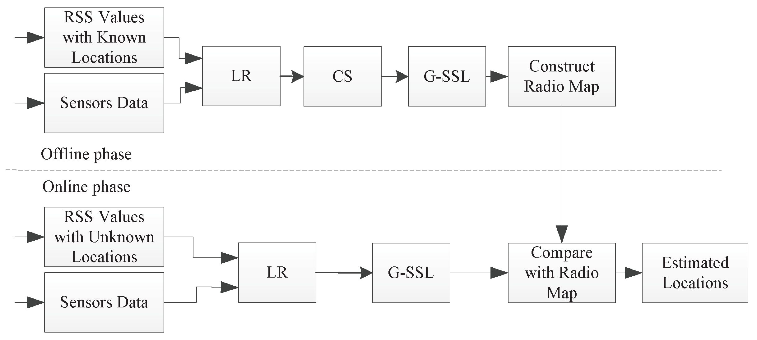
The proposed G-SSL-based RSS smoothing method for crowdsourcing is summarized in the system diagram shown in Figure 3. In the offline phase, since the actual coordinates of and are already known, the LR algorithm is used to obtain the uniform RSS values. Then the locations’ APs are calculated by CS method. At last the RSS values can be smoothed by G-SSL method. In the online phase, the data collected simultaneously from sensors on the mobile device can be used to estimate the relative displacement between and , that is, the distance . Then the collected RSS values are processed by the LR method. After that, the RSS values can be smoothed using the calculated distance . Finally, we get a more accurate positioning result.
4. Linear Regression Algorithm against Device Diversity Problem
In the existing experimental systems, the same device is used to collect the RSS values in both the offline phase and the online phase. However, when the crowdsourcing method is widely applied to the indoor localization systems, a large number of different mobile devices have been used in the establishment of the radio map. In the online phase, a variety of mobile devices are also used by the users which are different from the device used to build the radio map. In this section, the linear regression (LR) algorithm is proposed to solve the device diversity problem in RSS-based crowdsourcing localization system.
We define and are the signal space of different devices. Assume that the fingerprint belongs to is the nearest neighbor to the online point belongs to . As described above, although they were collected at close physical locations, the RSS values have obvious difference. In order to solve the device diversity problem, the relationship between different devices has to be studied. Therefore, these RSS values collected by different devices could be processed to make the in closer to . Mathematically
By learning f, the radio map build by the training device could be used to localize any other devices.
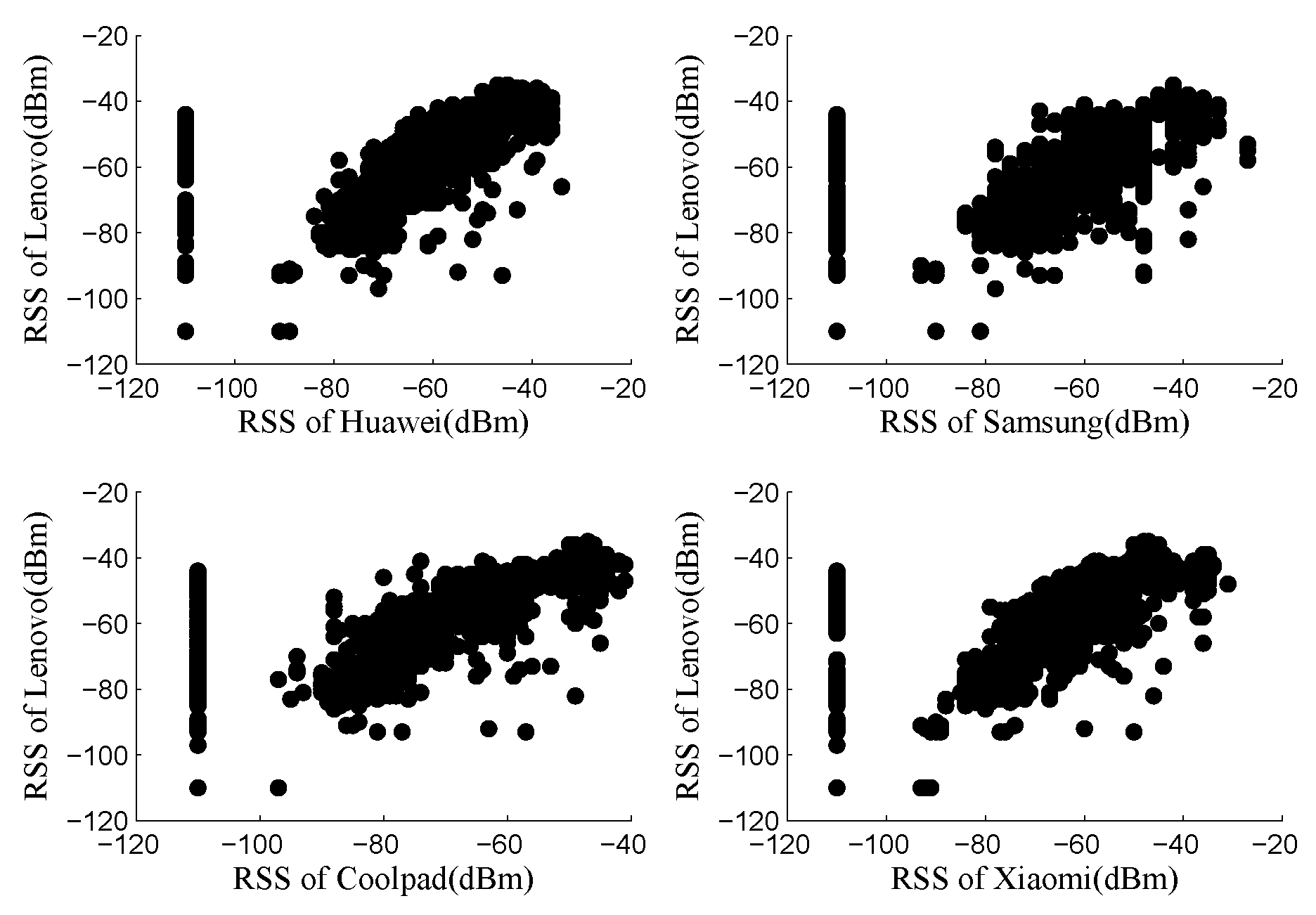
Aiming to explore the mapping function between RSS values collected by distinct devices, the comparison results of RSS values across different training/tracking devices are plotted in Figure 4. Every point on the figure represents RSS values from two different devices measured at the same location from the same AP at the same location. For example, the top right subplot in Figure 4 represents the RSS values measured by Lenovo laptop and Huawei mobile device. From Figure 4, we can get a linear correlation between the RSS values measured by different devices. Hence, the following linear regression method can be employed as the mapping function.
where are the coefficients in the mapping function.
4.1. Pre-Processing of RSS Values
In the typical WLAN localization scenario, the RSS values collected by the mobile device are subject to multiple sources of noise, such as multi-path fading and shadowing. To mitigate these RSS fluctuations, a large number of RSS measurements are collected from each AP at every location. Let be the set of RSS values collected at location l from the i-th AP. As shown in Figure 4, if we cannot receive any power from the AP, a value of dBm is used to denote the missing RSS value.
In order to obtain the high localization accuracy, the first step in localization system is to stabilize the collected RSS values prior to the localization process. Aiming to overcome the fluctuations, the average of the collected RSS values is calculated. In the calculation of the average value, the filled RSS values of could produce meaningless RSS values and will have a adverse impact. These filled RSS values could affect the localization process and produce erroneous location estimations. As a result, the average is calculated using the collected RSS values exclude the filled RSS values as the following equation:
where is an indicator function.
The average value is used to build the radio map in offline training phase and estimate the current location in online localization phase.
4.2. Linear Regression Algorithm against Device Diversity Problem
Before using the linear regression method, the parameters a and b in Equation 6 should be computed. Since the outliers appear in the collected RSS values frequently and seriously affect the performance of the linear least squares (LLS) algorithm, the fast least trimmed squares (FAST-LTS) algorithm is used in this paper.
When the number of measured RSS values is c, the FAST-LTS solution for linear regression with intercept is given by
where , and is norm 2 of a vector, are the ordered squared residuals: .
Given the h-subset of all nearest neighbors, the C-step is used to compute the a and b as follows [27]:
- compute and least squares regression estimator based on
- compute the residuals for
- sort the absolute values of these residuals,
- arrange the absolute values of the residuals in ascending order, let be a subset consisting of the nearest neighbors corresponding to the first h the absolute values of the residuals in the sequence
- compute and least squares regression estimator based on
Repeating C-step with numerous , a lot of regression coefficients will be gotten. The approximate solution is the coefficient corresponding to the least . After getting the regression coefficient a and b, is transformed as follows
where . As a result, both and belong to the same signal space, and a uniform radio map could be built using and in the offline training phase and a higher positioning accuracy could be obtained in online phase.
To verify the LR method, five distinct devices, namely Lenovo, Huawei, Samsung, Xiaomi and Coolpad, are used to collect RSS values at all RPs and the linear regression coefficients could be calculated based on the measured RSS values and the corresponding coordinates. When the regression coefficients are gotten, all the RSS values could be mapped into the same signal space by LR method and a uniform radio map could be built. Using the processed radio map, the user’s location will be estimated with a high accuracy in online phase.
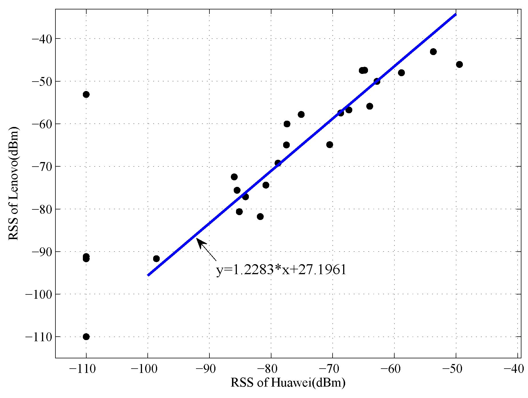
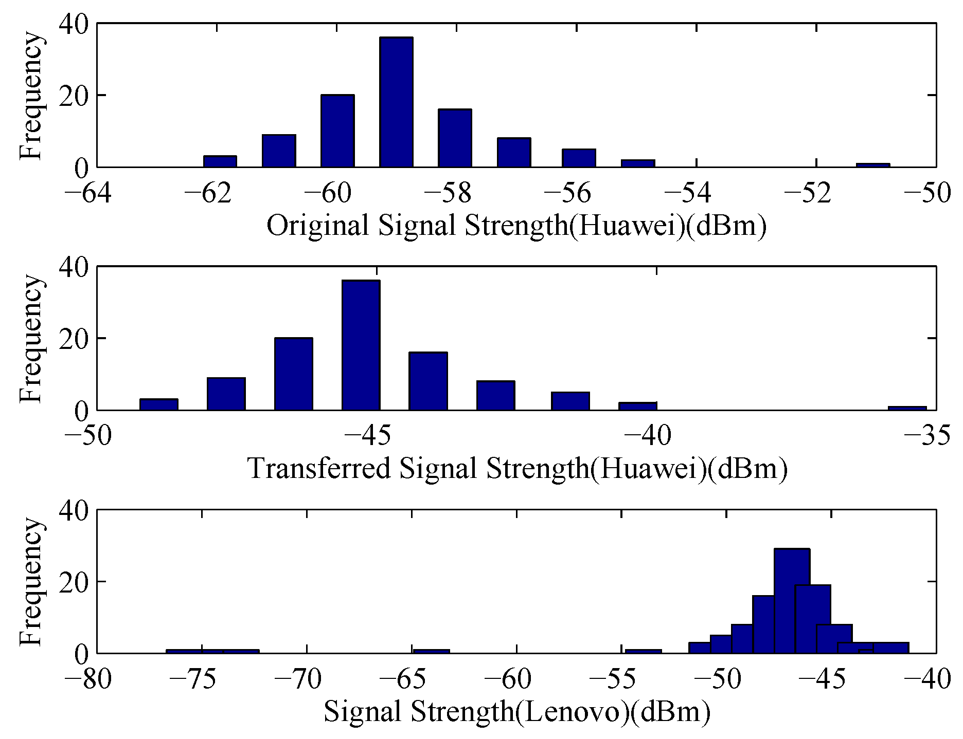
In our localization systems, we use the Lenovo device as the standard device, and all the RSS values collected by other devices are mapped into the signal space of Lenovo device. We take the (Huawei, Lenovo) pair as an example. As shown in Figure 5, the collected data are more stable after pre-processing of RSS values, and the linear regression coefficients could be calculated by LTS method. Using the coefficients, the RSS values collected by Huawei device could be mapped into the signal space of Lenovo device. We compare the original RSS values and the transferred RSS values collected by Lenovo device with the RSS values collected by the Lenovo device, the comparison result is shown in Figure 6. From the figure, we can see that the difference of signal distribution between different devices is reduced significantly. Accordingly, a uniform radio map can be built in the offline phase and the positioning performance could be improved in the online phase.
4.3. Automatic Device-Transparent Algorithm for Crowdsourcing Indoor Localization System
Based on the LR method, the device diversity problem can be solved. However, the LR method is applied to the premise that the coordinates of the RSS values are same. In offline training phase, the RSS values used to build the radio map have been labeled, so these RSS values meet the prerequisites for the LR method and the device diversity problem could be solved automatically. In online localization phase, the coordinates of the RSS values are unknown, which means the LR method cannot be used directly. Therefore, we use the correlation ratio computed from the Pearson Product-moment correlation coefficient to roughly label the RSS values collected by an unknown device.
where m is the number of APs, and are the RSS values measured from the k-th AP, is the average of the RSS values from the tracking device and is the mean of RSS values measured by the training device in a fingerprint.
The range of the absolute value of Pearson correlation ratio is where 1 indicates the highest linear correlation between RSS values and 0 indicates the least similarity. In the online phase, when the RSS vector is acquired, the similarity between the online point and all fingerprints in can be obtained by t. Given a threshold , we can get the set of nearest neighbor fingerprints in radio map for .
Based on the nearest neighbors in Equation (12), the RSS data collected in the online phase can be labeled roughly and the LR method proposed in the previous section is used to train the mapping function.
In summary, in the offline phase, because the coordinates of the collected RSS data are already known, the LR algorithm can be used to eliminate the device diversity problem directly. As a result, a uniform radio map can be built in the offline phase. In the online phase, the RSS values collected by the unknown device could be localized roughly by the Pearson correlation coefficient at the beginning. Then the RSS values can be mapped into the signal space of radio map using the LR algorithm. Finally, we can get a more accurate positioning result.
5. AP Localization Using Compressed Sensing Method
Typically, fingerprint-based localization methods do not rely on the location of the APs. In other words, the AP locations are assumed to be unknown. Nonetheless, better localization can be achieved if one could estimate the AP locations. Next, we discuss a compressed-sensing (CS)-based approach to estimate the AP locations.
Consider a set of N discrete locations throughout the indoor area. Suppose a set of M access points can be seen at each location. It is a practical assumption that the number of grid points is much larger than the number of access point in the indoor area i.e., . We will use this assumption to apply a CS-based method to recover the location of the APs.
Compressed Sensing is a signal processing technique that can efficiently reconstruct a signal by exploiting the sparsity and incoherence properties of the signal [28,29,30]. Assume corresponding to the i-th AP, we define a vector of size N. is a vector that shows the location of the AP by assigning a one to one the N element and zero for the rest of the element. For example, if then the location of the i-th AP is estimated to be the location of the n-th grid point in the indoor area. Concatenating all such vectors for all M APs results in a so-called index matrix, as,
According to the CS theory, rather than measuring the M-sparse signal or its sparse representation directly, compressive noisy RSS measurements in an ℓ-dimensional space are used. These compressive measurements are obtained by multiplying a random matrix by the original signal,
where
- are the compressive noisy RSS measurements.
- is the measurement matrix. Each row in this matrix represents the location of one RP, with an element of 1 to indicate the grid point at which the RP is located. Thus, only a few of RSS values are collected on the locations of RPs instead of measuring all the RSS values on the overall grid, which reduces the workload in the offline phase.
- is the sparsity basis on which the measured signals have sparse coefficients . In this matrix, indicates the RSS values collected at grid point i from the AP located at grip point j, for all and . Assume that the transmition power of an AP is . Then is calculated based on the empirical indoor propagation model of [20]:where d is the physical distance from the transmitter (AP) to the receiver.
- is the measurement noise.
The locations of the APs can be recovered by the following -minimization:
Unfortunately, solving (16) is both numerically unstable and NP-hard. Therefore, -minimization is used to recover the AP locations:
This is a convex optimization problem and various methods have been proposed to find the solution such as BP [31], OMP [32] and SP [33]. In this paper, we use OMP algorithm.
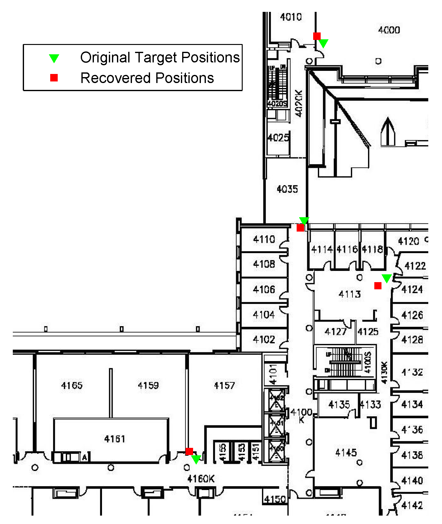
To evaluate the performance of the proposed CS-based AP localization algorithm, a few number of APs on the fourth floor of the Bahen Building at the University of Toronto have been localized. Figure 7 shows the AP localization results. As seen in the figure, all the AP locations are estimated with a high level of accuracy. Although the localization results contain some errors, it brings limited effect to our RSS smoothing method proposed later.
6. RSS Difference-Aware Graph-Based Semi-Supervised Learning RSS Smoothing Method
The G-SSL method tries to set the same value for and if the coordinates and at locations and are similar. However, since the distance between each RP and each of the unlabelled locations is known, we can use this information to estimate the expected difference in RSS based on the known locations of the APs and the radio propagation model. Thus, we define as the estimated RSS difference between and at location and . We change the smoothing constraint to reflect that the difference of estimated RSS values and should be close to . Accordingly, (4) can be written as:
6.1. Estimation of
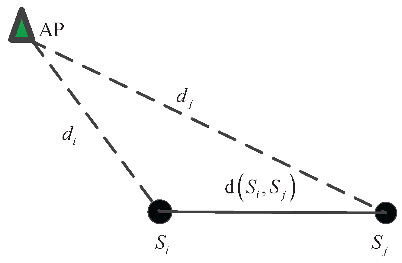
Consider one of the APs as shown in Figure 8. The location of the AP, , can be estimated using the CS-based method in [20]. We use the indoor signal propagation model in [34]. Therefore, the RSS value at location can be calculated as,
6.1.1. Offline Training Phase
In the offline training phase, the coordinates of RPs and , and , are already given in the radio map and the location of AP can be calculated precisely using the CS-based method. Thus, the Euclidean distance and between the RPs and AP can be obtained. Finally, the RSS difference can be calculated directly using (20).
6.1.2. Online Localization Phase
In the online localization phase, since the actual location of is unknown, cannot be calculated directly. However, can be estimated using inertial sensor data and step counting algorithms and can then be calculated. We can use (the mobile device moves towards AP) or (the mobile device moves away from AP) instead.
6.2. Finding the Optimal Solution
The cost function in (18) can be written as:
In order to find the optimal solution, we need to find the derivative of the cost function with respect to . Since the cost function of (21) is not convex, we use the gradient descent method to solve the optimization problem. Next, we derive the derivative for each part of the cost function in (21). The first part of (21) can be written as:
where is the RSS matrix and if the labels are not given, we use instead. is a Hermitian indication matrix where means that the corresponding i-th node in the graph is labelled and otherwise. Using (22), can be written as:
The second part of (21) can rearranged as:
where is the graph Laplacian and where for all . Differentiating yields,
The derivative of the third part of the cost with respect to is equal to 0. The last part of (21) is:
where . In order to find , first we find for . Using [34],
Since , . Therefore:
where and is obtained using:
where . Finally, in order to find the optimal solution, we set :
Using (23), (25) and (29):
In summary, to find the optimal solution, initialize . Then use an iterative procedure as follows: First, find as the solution of (31). Second, update based on the result of the first step and the definition of . Repeat the two steps until convergence.
6.3. Experimental Results
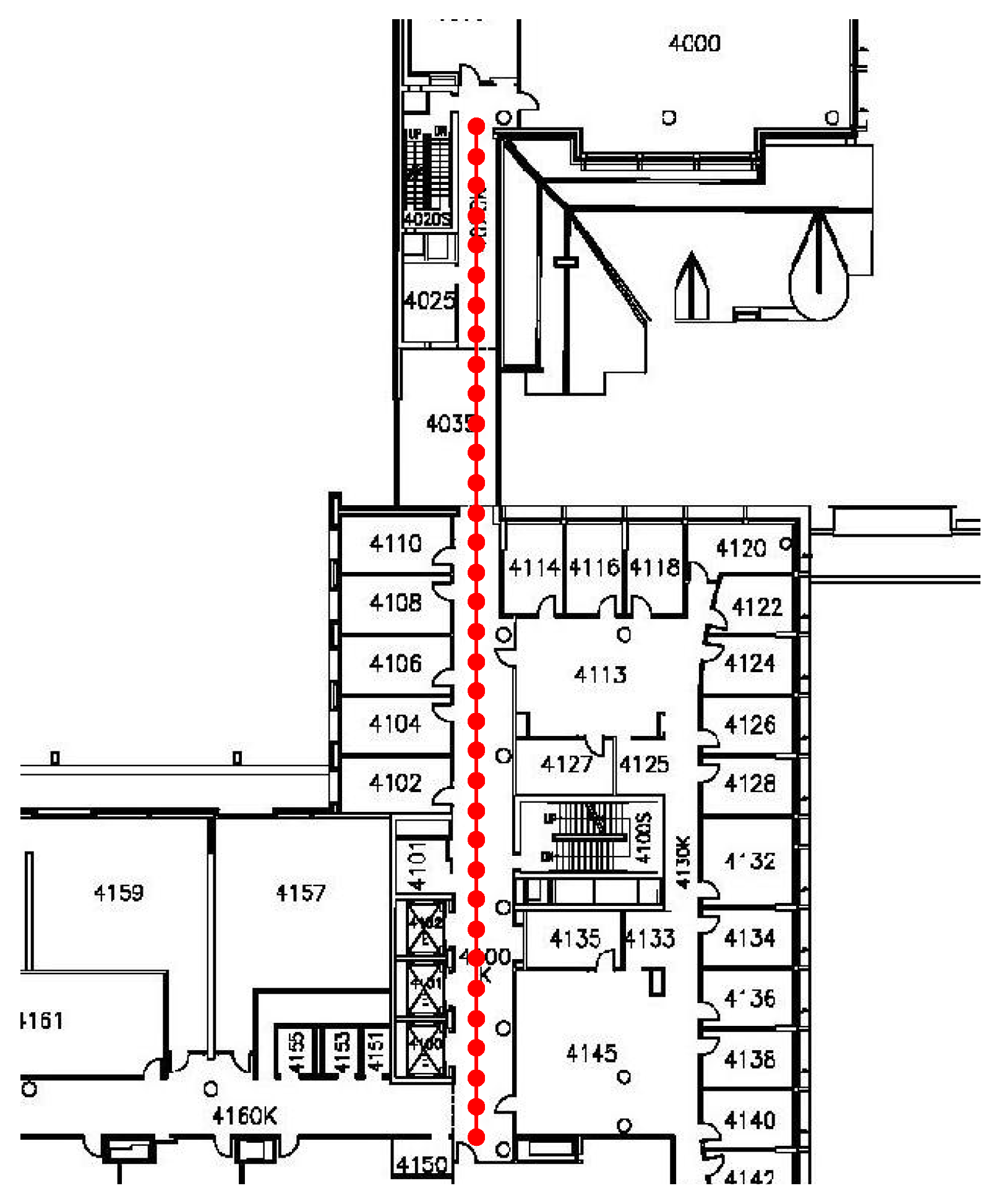
In order to verify our method, we collected RSS data from the 4th floor of the Bahen Building at the University of Toronto. The radio map was constructed using a step-counter-assisted RSS measurement method. Sensor information from the accelerometer is used to estimate the distance between the RPs. Using this system, a radio map consisting of 251 RPs throughout the entire 4th floor of the Bahen building has been created in less than 30 minutes. However, the resulting radio map has only 5 RSS measurements at each RP. Consequently, it is more error-prone compared to the traditionally generated radio maps in which for each RP hundreds of measurements are collected. The Proposed localization procedure is tested on a sequence of 35 test points collected on a path from Room 4000 (top of Figure 9) to Room 4148 (bottom of Figure 9).
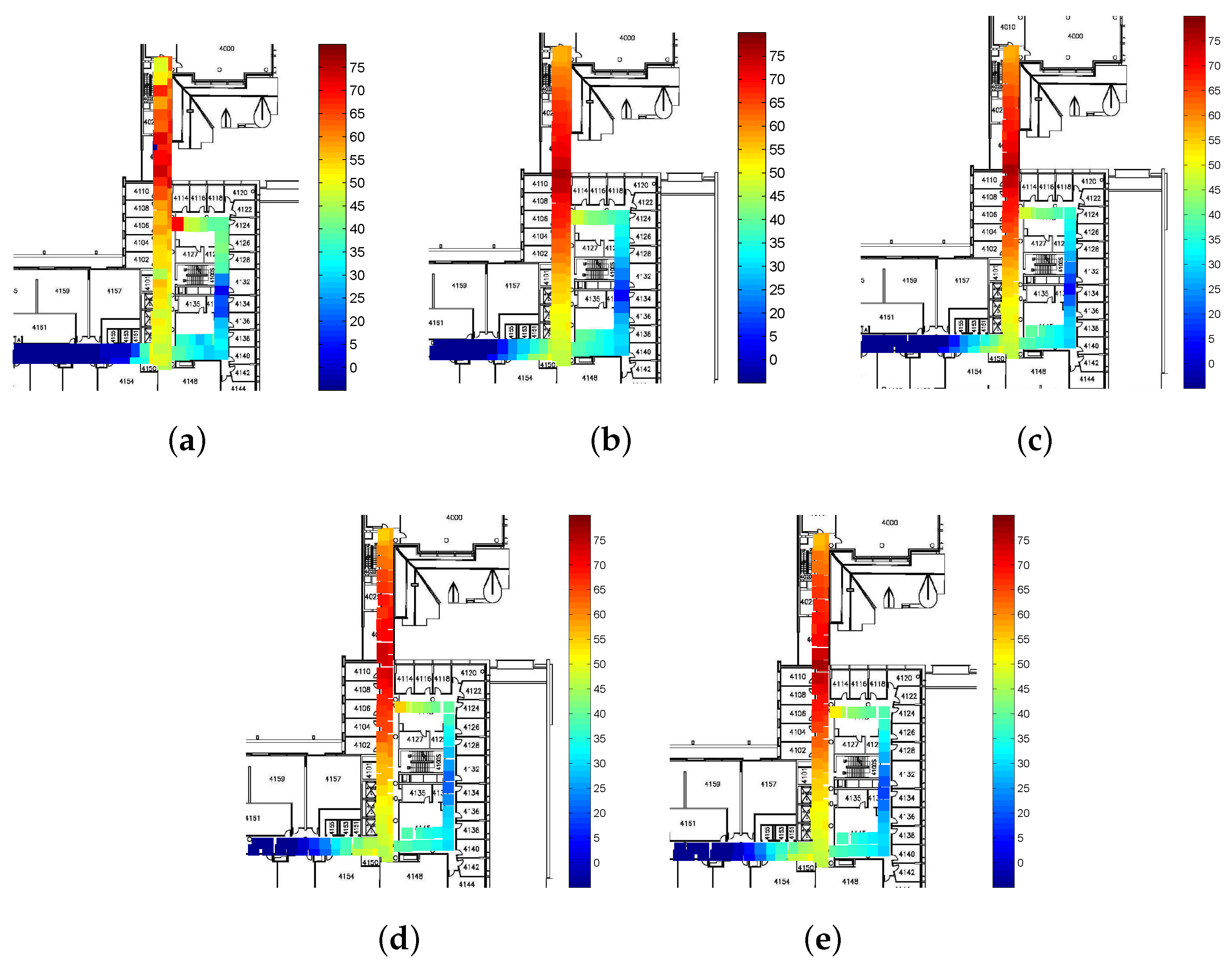
The RSS values from a single AP in the original radio map and the test points are shown in Figure 10a and Figure 11a respectively. As can be seen, although the RSS values are generally consistent with the signal propagation model, there are some large fluctuations at some RPs. To eliminate the negative effects caused by this fluctuation, the proposed RG-SSL method is applied to smooth the RSS values. In order to obtain more accurate results, 125 unlabelled data throughout the whole 4th floor of the Bahen Building are considered. Following steps are repeated until all the labelled points are smoothed:
- Set one of the labelled points as unlabelled.
- Use the rest of the labelled points, 125 unlabelled points and RG-SSL method to estimate the RSS value of the above unlabelled point.
As comparisons, the G-SSL method, SCTW method and SPORT method are also simulated in this paper. The simulation results are shown in Figure 10 and Figure 11. From Figure 10b and Figure 11b we can see that the RG-SSL method successfully smooths out the radio map and the effect of signal fluctuation is mitigated. Because most of the information in the radio map is abandoned in the SCTW algorithm, it cannot achieve the optimal result. In the SPORT algorithm, due to the variability of the parameters in the signal propagation model, we can obtain suboptimal solution of the RSS values rather than the best results. In the G-SSL algorithm, all the collected RSS values are used to correct the outliers, which leads to a better result. Furthermore, the RSS difference between different locations is used to improve the G-SSL method and the estimated RSS values are more accurate. As a result, although the radio map and the online RSS values are also smoothed by the other algorithms, the errors are larger than that in Figure 10b and Figure 11b, especially in the upper part of the corridor. The increasing errors in RSS values in the radio map and the online data will inevitably result in the increased localization errors.
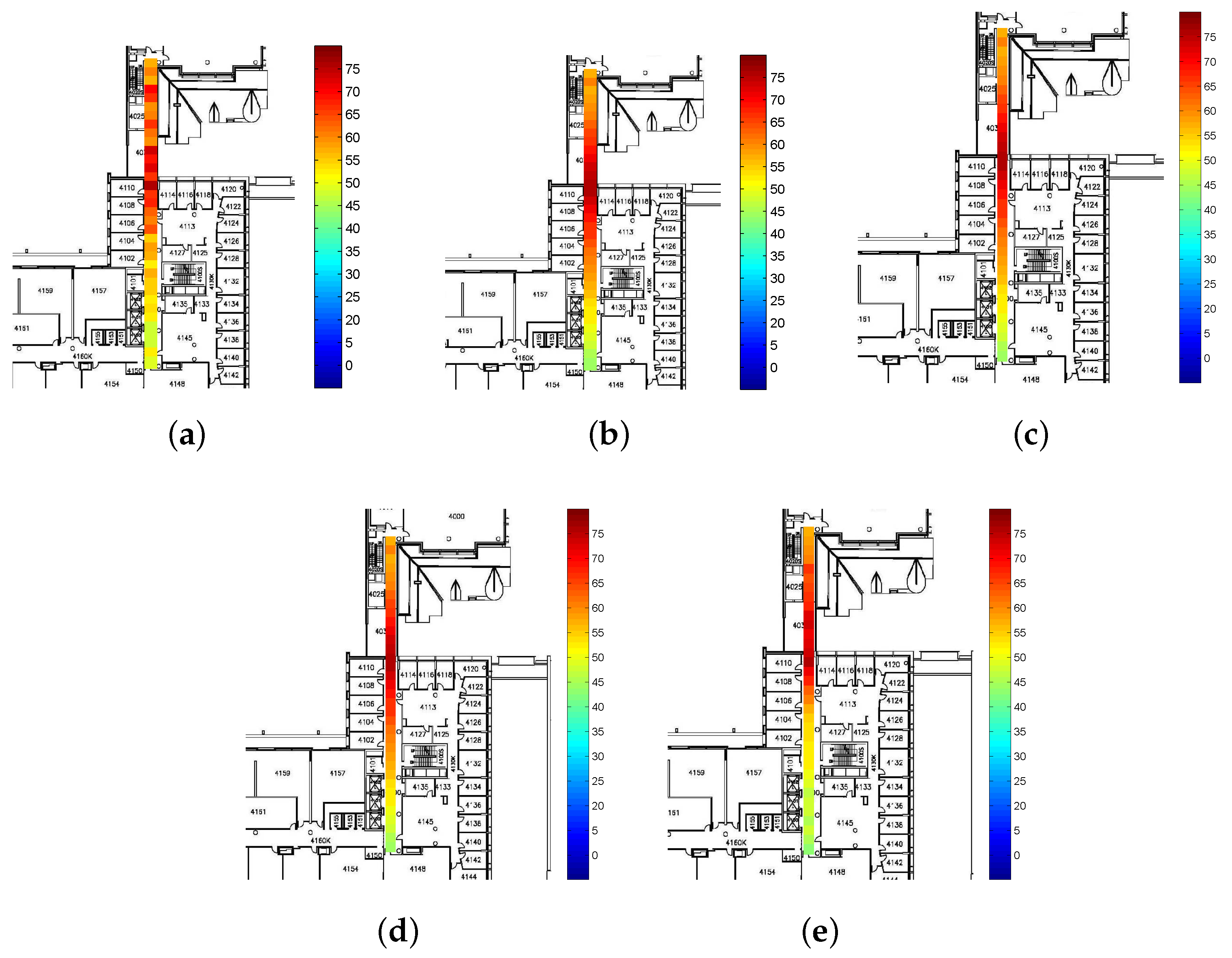
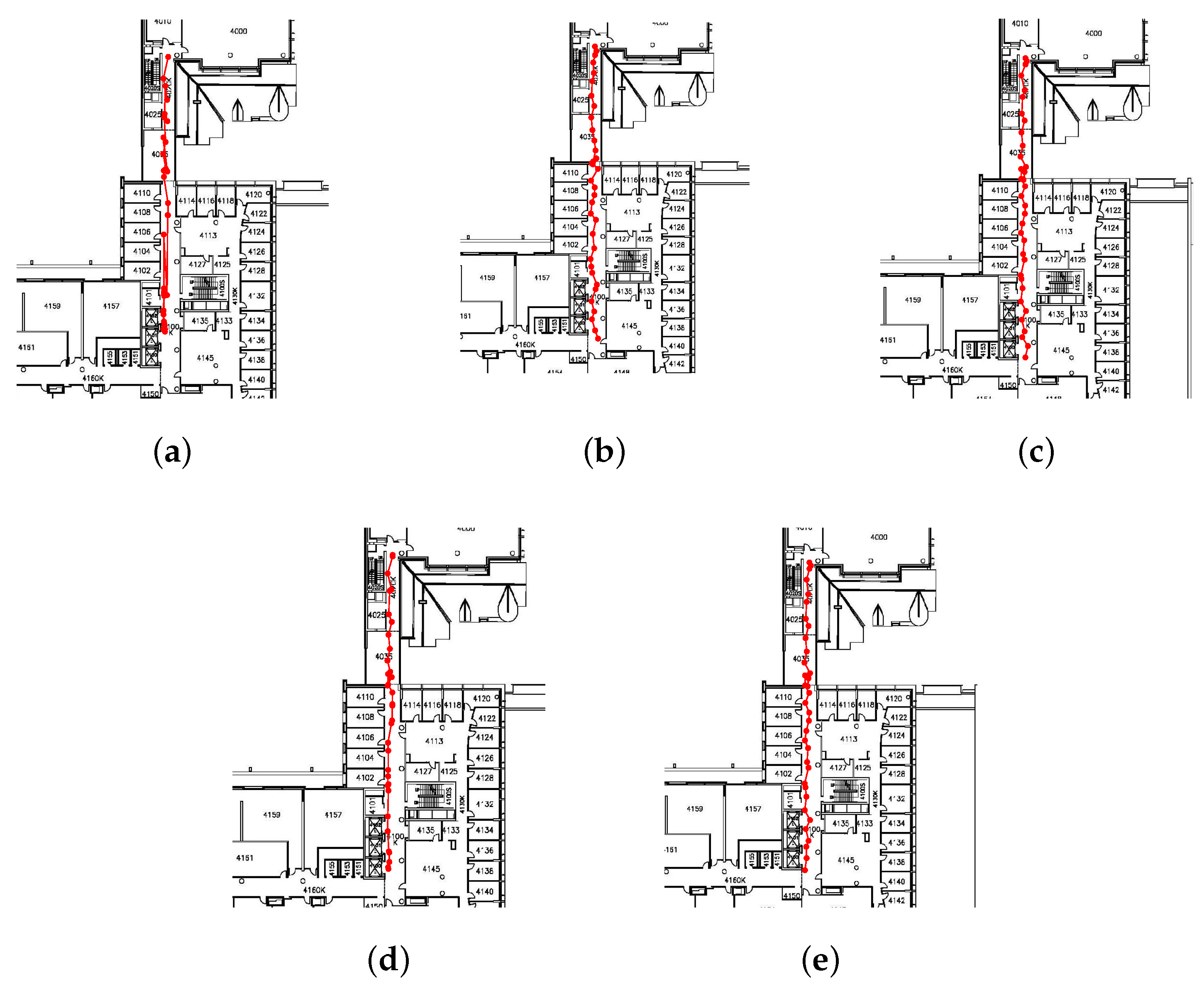
The localization result from directly using the original radio map and test point data are shown in Figure 12a. Compared with the actual locations in Figure 9, there are some significant errors in the localization results as certain distinct test points have been localized erroneously to a single location. The localization result using the modified radio map can be seen in Figure 12b–e. We see that the localization results are improved compared to the results in Figure 12a. Most of the test points were erroneously localized to one location in Figure 12a are now localized to correct distinct locations. These incorrect estimates were causing a large amount of localization error in the original method however are greatly reduced using both the RG-SSL method and the other methods. Clearly, the localization results of the proposed RG-SSL method are closer to actual locations than the results calculated by the other methods. Furthermore, the trajectory obtained in Figure 12b is clearly smoother than those in Figure 12c–e.
We can readily see the performance gain of the RG-SSL method in the cumulative distribution function (CDF) of the localization error for the RG-SSL method and the other methods, as shown in Figure 13 and Table 1. It is clear that the proposed localization method outperforms the other methods. As discussed above, the RSS values smoothed by RG-SSL are more accurate than those smoothed by the other algorithms, and the location accuracy is increased by 3.5% relative to G-SSL and SPORT, 9.8% compared to SCTW method and 20.6% relative to original data. The average localization error has been reduced from 2.89 m to 2.07 m, and notably, the maximum localization error has been reduced from 10 m to 4 m.
7. RSS Difference-Aware Sparse Graph-Based Semi-Supervised Learning Method and Experimental Results
7.1. Sparse Graph Construction for RG-SSL Using CS Method
Since the radio map is constructed using a step-counter-assisted RSS measurement method, the coordinate of each RP calculated by this method contains a lot of noise. In the proposed RG-SSL method, the heat-kernel function is used to construct the graph and calculate the edge weights based on the Euclidean distance. However, the Euclidean distance and consequently the weights are very sensitive to noise.
The accuracy of the generated graph will greatly affect the positioning performance. When the vertices in the graph are far away from each other, the graph weight is much smaller than the graph weight calculated for neighboring vertices. Therefore, the graph weight matrix is sparse. Since the CS method is robust to noisy data, we can use it to estimate the graph weight matrix [35]. As mentioned in Section 2, we denote the vertex set . Given the measurement matrix and the matrix for unknown reconstruction coefficients we can reconstruct a sparse from using:
where denotes the -norm. The -norm minimization is NP-hard. However, if the solution is sparse enough, the following convex -norm minimization can be used to solve the sparse representation problem:
Suppose the noise in the collected RSS is denoted by . Then,
where and . Thus the -norm minimization can be rewritten as:
For each in the vertex set, the measurement matrix is constructed as and is calculated using -norm minimization:
where is the i-th column of the matrix . Then the graph weights are obtained using:
where and denotes the j-th element of vector .
7.2. Experimental Results
Since the labels of all the vertices in the graph are necessary for sparse reconstruction of the graph weight matrix, CS method can only be used in the offline phase. The weighted matrices calculated by the heat-kernel function and CS method are shown in Figure 14a,b, respectively. Each pixel in the figure represents the weight value between two vertices and . A larger value of between vertex and means a stronger correlation between them. If the vertices around the vertex have strong correlations with the vertex , we can get a more accurate RSS estimates for the vertex . As we can see from Figure 14a, since the measurements are noisy, the weight matrix contains some errors. In the weight matrix, the weight values are very small between different vertices, which means the relationship between different vertices is very weak. Therefore, the information transferred between different vertices is inaccurate and the estimated RSS values using this weight matrix are not accurate enough. As a result, the localization accuracy is reduced by the inaccurate relationship between different locations.
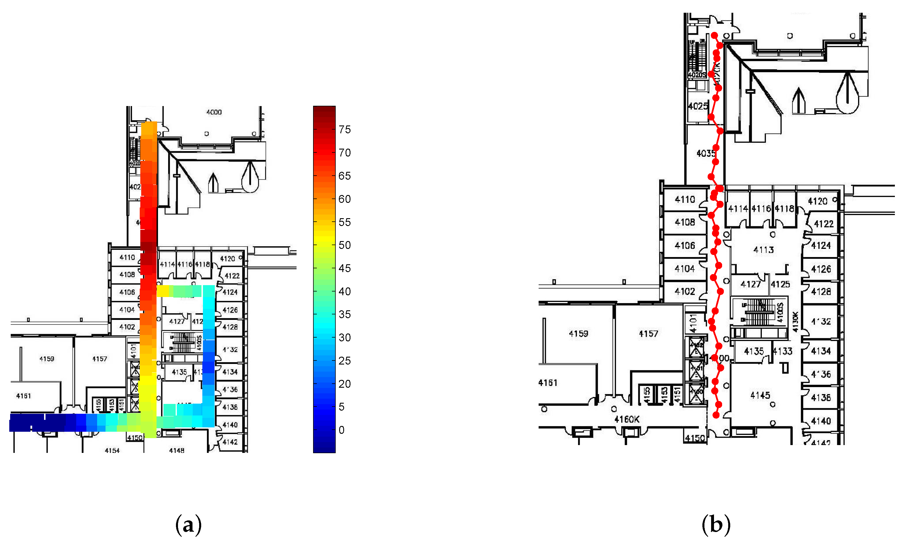
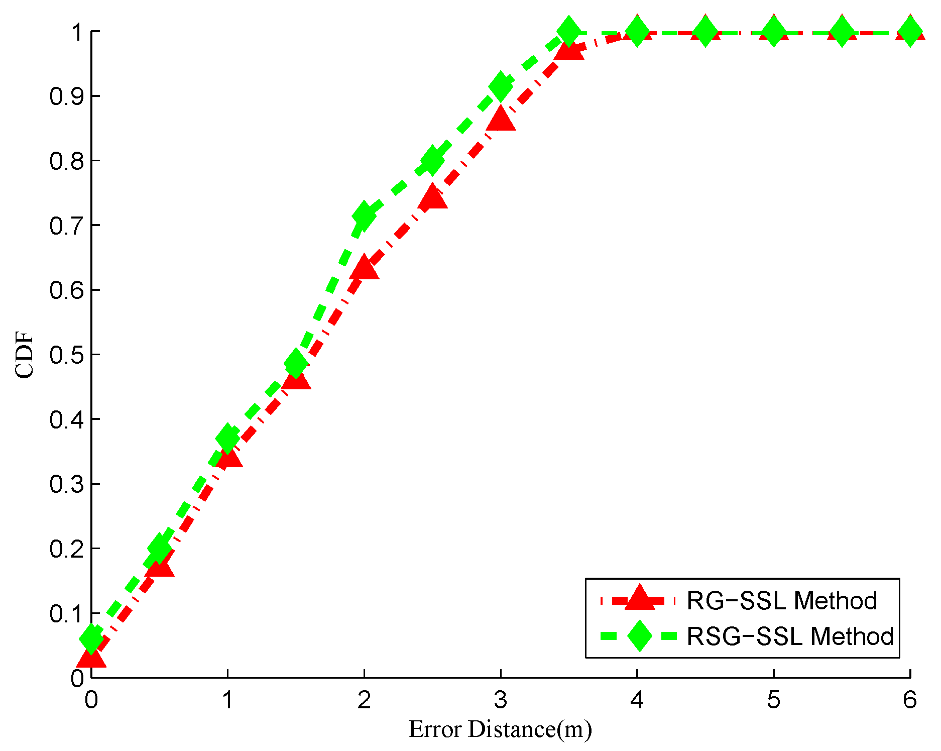
Due to the sparsity of the graph and robustness to noise, the weight matrix is recovered more precisely than the traditional heat-kernel function. The relationship between different vertices in Figure 14b is much clearer than Figure 14a. Comparing Figure 14b with Figure 14a, the graph weight values calculated by the CS method are much larger than those obtained using the heat-kernel. As a result, it is possible to get more useful information between different vertices using the matrix in Figure 14b. Therefore, the estimated RSS values are more accurate than those calculated by the heat-kernel as shown in Figure 15a,b. Based on the matrix calculated by the CS method, the localization results are more accurate in Figure 15b. From Figure 16 we can learn that the cumulative probability is 71.4% when the location error is 2 m and the localization accuracy is increased by 7.9% relative to RG-SSL, 11.5% relative to G-SSL and SPORT, 17.1% compared to SCTW algorithm. Thanks to the more accurate radio map, the maximum localization error has been further reduced to 3.5 m. Meanwhile, the average localization error has been reduced from 2.07 m to 1.98 m. In summary, the RSG-SSL algorithm is more robust to noise and has achieved a better performance than RG-SSL algorithm and much better than other algorithms. By using the RSG-SSL method, the localization accuracy is improved significantly in crowdsourcing WLAN indoor localization system. As a result, the localization system could provide us with much better service.
8. Conclusions
In this paper, the effect of noise and erroneous measurements caused by the crowdsourced data are reduced using the relationship between RSS values of different locations. The LR method is used to solve the device diversity problem automatically in crowdsourcing system at the beginning. After getting the uniform radio map, the RG-SSL method is proposed to improve the localization accuracy by smoothing the RSS values and using label propagation to better estimate the radio map. The relationship between the RSS values is represented using a weighted graph connecting different locations. Additionally, the RSS difference is introduced in the traditional G-SSL method to achieve a better performance. In order to obtain the RSS difference, a CS-based method is used to precisely localize the location of the APs. Noisy RSS values can be corrected using the proposed RG-SSL method, resulting in a higher localization accuracy. Due to the sparsity of the weighted graph in the G-SSL, the weighted graph is reconstructed more accurately by the CS method compared to the traditional heat-kernel function which is the idea of the proposed RSG-SSL method. The experimental results performed at the University of Toronto show that a smoothed radio map and online RSS values are obtained by RG-SSL method and the localization accuracy is improved. The RSG-SSL method applied in the offline phase also resulted in an improved performance.
Acknowledgments
This paper is supported by National Natural Science Foundation of China (61571162), Natural Science Foundation of Hei Longjiang Province China (F2016019), Postdoctoral Science-Research Development Foundation of Hei Longjiang Province China (LBH-Q12080), and Science and Technology Project of Ministry of China Public Security Foundation (2015GABJC38).
Author Contributions
Liye Zhang, Shahrokh Valaee, Yubin Xu and Lin Ma conceived the idea of the paper; Liye Zhang designed and performed the experiments; Shahrokh Valaee, Yubin Xu and Lin Ma analyzed the data; Liye Zhang wrote the paper; Shahrokh Valaee, Farhang Vedadi, Yubin Xu and Lin Ma revised the paper.
Conflicts of Interest
The authors declare no conflict of interest.
Abbreviations
The following abbreviations are used in this manuscript:
| MDPI | Multidisciplinary Digital Publishing Institute |
| DOAJ | Directory of open access journals |
| TLA | Three letter acronym |
| LD | linear dichroism |
References
- Sorour, S.; Lostanlen, Y.; Valaee, S.; Majeed, K. Joint indoor localization an radio map construction wiht limited deployment load. IEEE Trans. Mob. Comput. 2015, 14, 1031–1043. [Google Scholar] [CrossRef]
- Feng, C.; Valaee, S.; Au, A.W.S.; Tan, Z. Received-signal-strength-based indoor positioning using compressive sensing. IEEE Trans. Mob. Comput. 2012, 11, 1983–1993. [Google Scholar] [CrossRef]
- Gu, Y.; Lo, A.; Niemegeers, I. A survey of indoor positioning systems for wireless personal network. IEEE Commun. Surv. Tutor. 2009, 11, 13–32. [Google Scholar] [CrossRef]
- Alarifi, A.; Al-Salman, A.; Alsaleh, M.; Alnafessah, A.; Al-Hadhrami, S.; Al-Ammar, M.A.; Al-Khalifa, H.S. Ultra Wideband Indoor Positioning Technologies: Analysis and Recent Advances. Sensors 2016, 16, 707. [Google Scholar] [CrossRef] [PubMed]
- Feng, C.; Valaee, S.; Tan, Z. Localization of wireless sensors using compressive sensing for manifold learning. In Proceedings of the 2009 IEEE 20th International Symposium on Personal, Indoor and Mobile Radio Communications (PIMRC), Tokyo, Japan, 13–16 September 2009; pp. 2715–2719. [Google Scholar]
- Harle, R. A survey of indoor inertial positioning systems for pedestrians. IEEE Commun. Surv. Tutor. 2013, 15, 1281–1293. [Google Scholar] [CrossRef]
- Bahl, P.; Padmanabhan, V. Radar: An in-building RF-based user location and tracking system. In Proceedings of the 2000 Nineteenth Annual Joint Conference of the IEEE Computer and Communications Societies (INFOCOM), Tel Aviv, Israel, 26–30 March 2000; pp. 775–784. [Google Scholar]
- Kushki, A.; Plataniotis, K.N.; Venetsanopoulos, A.N. Kernel-based positioning in wireless local area networks. IEEE Trans. Mob. Comput. 2007, 6, 689–705. [Google Scholar] [CrossRef]
- Rai, A.; Chintalapudi, K.K.; Padmanabhan, V.N.; Sen, R. Zee: Zero-effort crowdsourcing for indoor localization. In Proceedings of the 18th Annual International conference on Mobile Computing Network, Istanbul, Turkey, 22–26 August 2012; pp. 293–304. [Google Scholar]
- Viel, B.; Asplund, M. Why is fingerprint-based indoor localization still so hard? In Proceedings of the 2014 IEEE International Conference on Pervasive Computing and Communications Workshops (PERCOM Workshops), Budapest, Hungary, 24–28 March 2014; pp. 443–448. [Google Scholar]
- Pan, J.J.; Pan, S.J.; Yin, J.; Ni, L.M.; Yang, Q. Tracking mobile users in wireless networks via semi-supervised colocalization. IEEE Trans. Pattern Anal. Mach. Intell. 2012, 34, 587–600. [Google Scholar] [CrossRef] [PubMed]
- Au, A.W.S.; Feng, C.; Valaee, S.; Reyes, S.; Sorour, S.; Markowitz, S.N.; Gold, D.; Gordon, K.; Eizenman, M. Indoor tracking and navigation using received signal strength and compressive sensing on a mobile device. IEEE Trans. Mob. Comput. 2013, 12, 2050–2062. [Google Scholar] [CrossRef]
- Redzic, M.; Brennan, C.; O’Connor, N. SEAMLOC: Seamless indoor localization based on reduced number of calibration points. IEEE Trans. Mob. Comput. 2014, 13, 1326–1337. [Google Scholar]
- Yang, S.; Dessai, P.; Verma, M.; Gerla, M. FreeLoc: Calibration-free crowdsourced indoor localization. In Proceedings of the 32nd IEEE International Conference on Computer Communications (INFOCOM), Turin, Italy, 14–19 April 2013; pp. 2481–2489. [Google Scholar]
- Wu, C.; Yang, Z.; Liu, Y. Smartphones based crowdsourcing for indoor localization. IEEE Trans. Mob. Comput. 2015, 14, 444–457. [Google Scholar] [CrossRef]
- Yu, N.; Xiao, C.; Wu, Y.; Feng, R. A Radio-Map Automatic Construction Algorithm Based on Crowdsourcing. Sensors 2016, 16, 504. [Google Scholar] [CrossRef] [PubMed]
- Kaemarungsi, K. Distribution of wlan received signal strength indication for indoor location determination. In Proceedings of the 1st International Symposium on Wireless Pervasive Computing, Phuket, Thailand, 16–18 January 2006; pp. 2952–2957. [Google Scholar]
- Zheng, V.W.; Pan, S.J.; Yang, Q.; Pan, J.J. Transferring Multi-device Localization Models using Latent Multi-task Learning. In Proceedings of the 23rd national conference on Artificial intelligence, Chicago, IL, USA, 13–17 July 2008; pp. 1427–1432. [Google Scholar]
- Tsui, A.W.; Chuang, Y.H.; Chu, H.H. Unsupervised Learning for Solving RSS Hardware Variance Problem in WiFi Localization. Mob. Netw. Appl. 2009, 14, 677–691. [Google Scholar] [CrossRef]
- Feng, C.; Valaee, S.; Tan, Z. Multiple Target Localization Using Compressive Sensing. In Proceedings of the 2009 IEEE Global Communications Conference (GLOBECOM), Honolulu, HI, USA, 30 November– 4 December 2009; pp. 1–6. [Google Scholar]
- Liu, X.D.; He, W.; Tian, Z.S. The improvement of RSS-based location fingerprint technology for cellular networks. In Proceedings of the 2012 International Conference on Computer Science and Service System (CSSS), Nanjing, China, 11–13 August 2012; pp. 1267–1270. [Google Scholar]
- Hasani, M.; Lohan, E.-S.; Sydanheimo, L.; Ukkonen, L. Path-loss model of embroidered passive RFID tag on human body for indoor positioning applications. In Proceedings of the 2014 IEEE RFID Technology and Applications Conference (RFID-TA), Tampere, Finland, 8–9 September 2014; pp. 170–174. [Google Scholar]
- Latif, S.; Memon, A.; Chawdhry, B.; Zielinski, R.; Khan, G. Accuracy Assessment of D-Model for Modeling Wall Attenuation in Indoor Environment. In Proceedings of the 2014 Sixth International Conference on Computational Intelligence, Communication Systems and Networks (CICSyN), Tetovo, Macedonia, 27–29 May 2014; pp. 71–76. [Google Scholar]
- Zhang, L.; Shahrokh, V.; Zhang, L.; Xu, Y.; Ma, L. Signal propagation-based outlier reduction technique (SPORT) for crowdsourcing in indoor localization using fingerprint. Proceedings of Personal, Indoor, and Mobile Radio Communications (PIMRC), 2015 IEEE 26th Annual International Symposium on, Hong Kong, China, 30 August–2 September 2015; pp. 2008–2013. [Google Scholar]
- Rahman Sakib, M.S.; Quyum, M.A.; Andersson, K.; Synnes, K.; Korner, U. Improving Wi-Fi based indoor positioning using Particle Filter based on signal strength. In Proceedings of the 2014 IEEE Ninth International Conference on Intelligent Sensors, Sensor Networks and Information Processing (ISSNIP), Singapore, 21–24 April 2014; pp. 1–6. [Google Scholar]
- Ma, L.; Xu, Y. Received signal strength recovery in green WLAN indoor positioning system using singular value threholding. Sensors 2015, 15, 1292–1311. [Google Scholar] [CrossRef] [PubMed]
- Rousseeuw, P.J.; Driessen, K.V. Computing LTS Regression for Large Data Sets. Data Min. Knowl. Discov. 2006, 12, 29–45. [Google Scholar] [CrossRef]
- Candès, E.J. Compressive sampling. In Proceedings of the international congress of mathematicians, Madrid, Spain, 22–30 August 2006; pp. 1433–1452. [Google Scholar]
- Baraniuk, R.G. Compressive sensing. IEEE Signal Proc. Mag. 2007, 24, 118–121. [Google Scholar] [CrossRef]
- Cande`s, E.J.; Wakin, M.B. An introdution to compressive sampling. IEEE Signal Proc. Mag. 2008, 25, 21–30. [Google Scholar] [CrossRef]
- Chen, S.S.; Donoho, D.L.; Saunders, M.A. Atomic decomposition by basis pursuit. SIAM J. Sci. Comput. 1998, 20, 33–61. [Google Scholar] [CrossRef]
- Tropp, J.; Gilbert, A. Signal Recovery from Random Measurements via Orthogonal Matching Pursuit. IEEE Trans. Inf. Theory 2008, 53, 4655–4666. [Google Scholar] [CrossRef]
- Dai, W.; Milenkovic, O. Subspace pursuit for compressive sensing signal reconstruction. IEEE Signal Proc. Mag. 2009, 55, 2230–2249. [Google Scholar] [CrossRef]
- Pourahmadi, V.; Valaee, S. Indoor Positioning and distance-aware graph-based semi-supervised learning method. In Proceedings of the 2012 IEEE Global Communications Conference (GLOBECOM), Anaheim, CA, USA, 3–7 December 2012; pp. 315–320. [Google Scholar]
- Cheng, B.; Yang, J.; Yan, S.; Fu, Y.; Huang, T.S. Learning with ℓ1-Graph for image analysis. IEEE Trans. Image Proc. 2010, 19, 858–866. [Google Scholar] [CrossRef] [PubMed]
Figure 1.
Histogram of 100 RSS values of a single AP measured at a location.
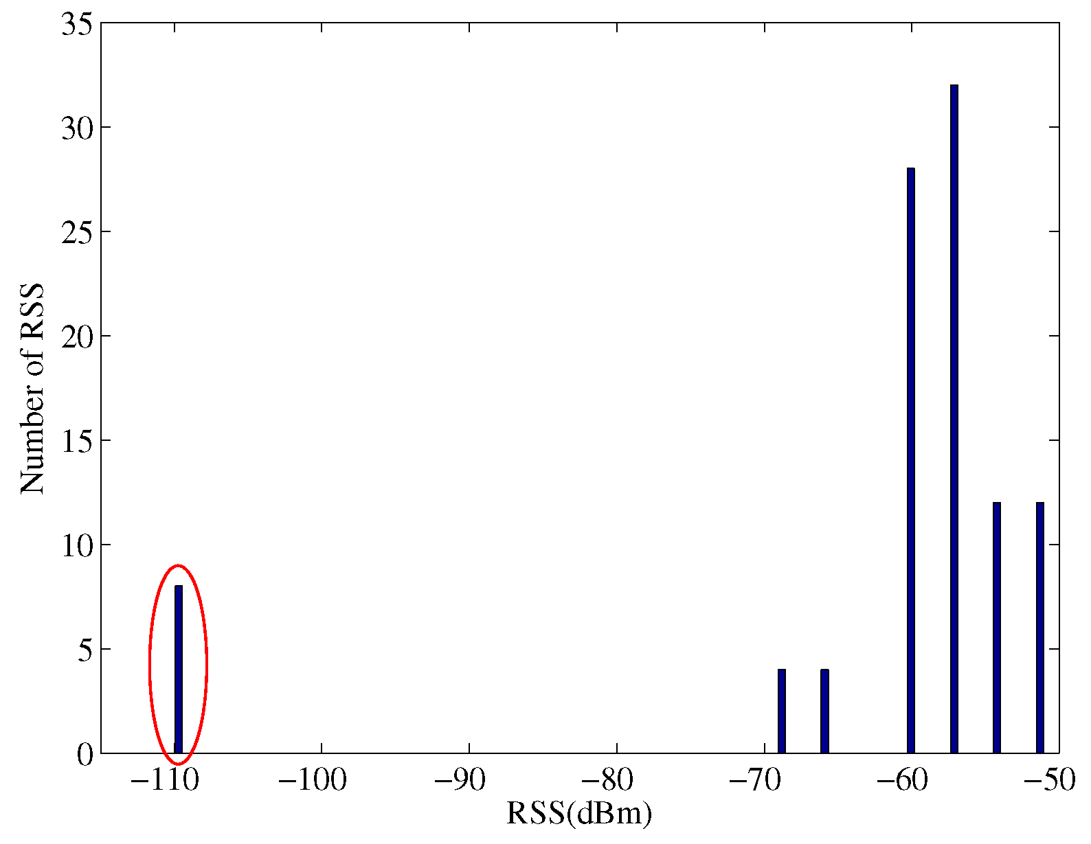
Figure 2.
RSS values of an AP over the corridor area of the fourth floor of the Bahen Building, University of Toronto.
Figure 2.
RSS values of an AP over the corridor area of the fourth floor of the Bahen Building, University of Toronto.
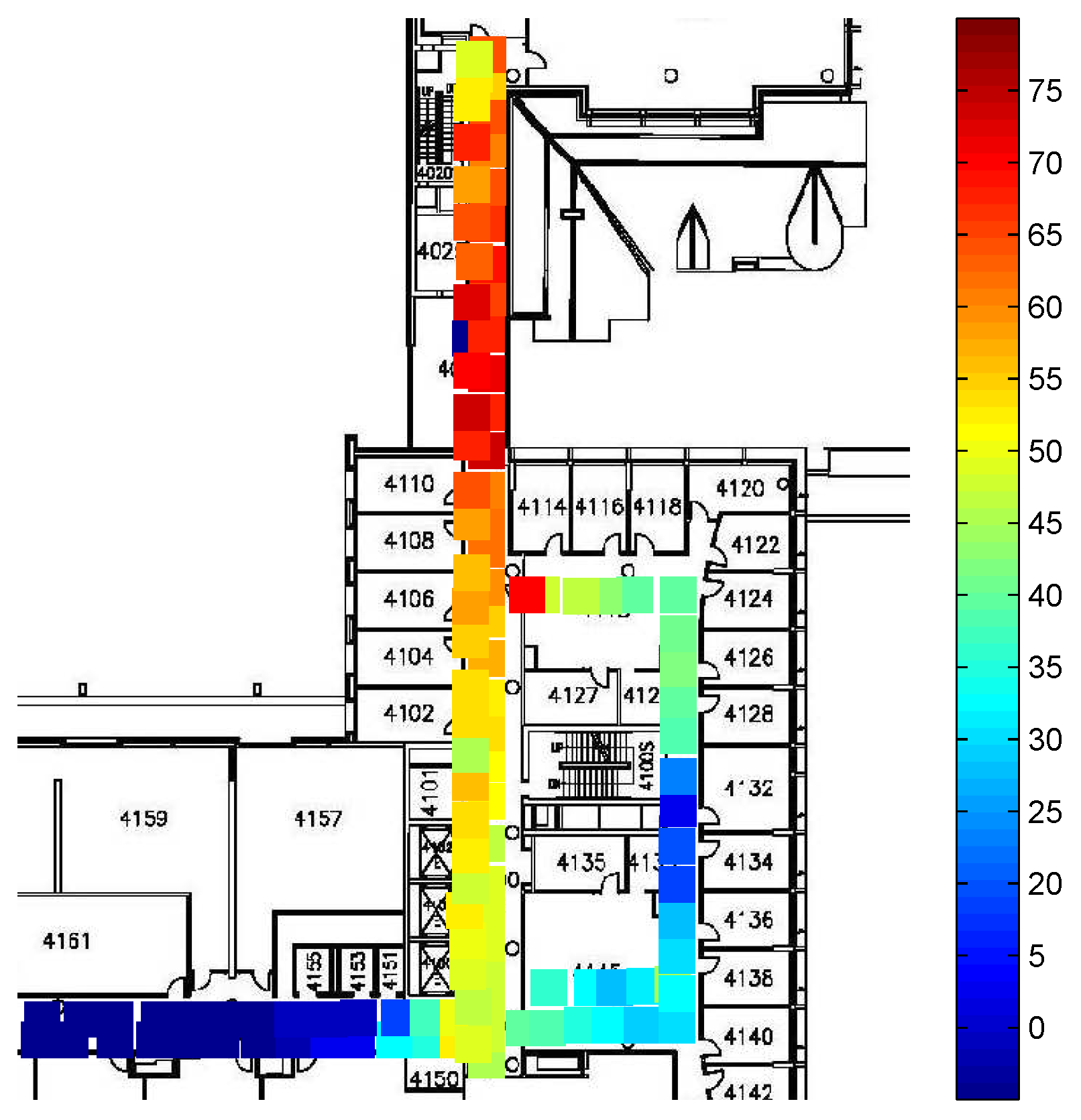
Figure 3.
The system view of the proposed G-SSL based Localization.

Figure 4.
Linear correlation between RSS values for different devices.

Figure 5.
Linear correlation between Lenovo and Huawei.

Figure 6.
Comparison of signal distribution.

Figure 7.
AP localization results using CS method.

Figure 8.
Mobile device is moving away from AP.

Figure 9.
Actual locations of test points.

Figure 10.
Comparison of signal distribution of radio map. (a) Original radio map (b) RG-SSL method (c) G-SSL method (d) SCTW method (e) SPORT method
Figure 10.
Comparison of signal distribution of radio map. (a) Original radio map (b) RG-SSL method (c) G-SSL method (d) SCTW method (e) SPORT method

Figure 11.
Comparison of signal distribution of test data. (a) Original radio map (b) RG-SSL method (c) G-SSL method (d) SCTW method (e) SPORT method
Figure 11.
Comparison of signal distribution of test data. (a) Original radio map (b) RG-SSL method (c) G-SSL method (d) SCTW method (e) SPORT method

Figure 12.
Comparison of localization results. (a) Original radio map (b) RG-SSL method (c) G-SSL method (d) SCTW method (e) SPORT method
Figure 12.
Comparison of localization results. (a) Original radio map (b) RG-SSL method (c) G-SSL method (d) SCTW method (e) SPORT method

Figure 13.
Cumulative distribution function of the localization error.
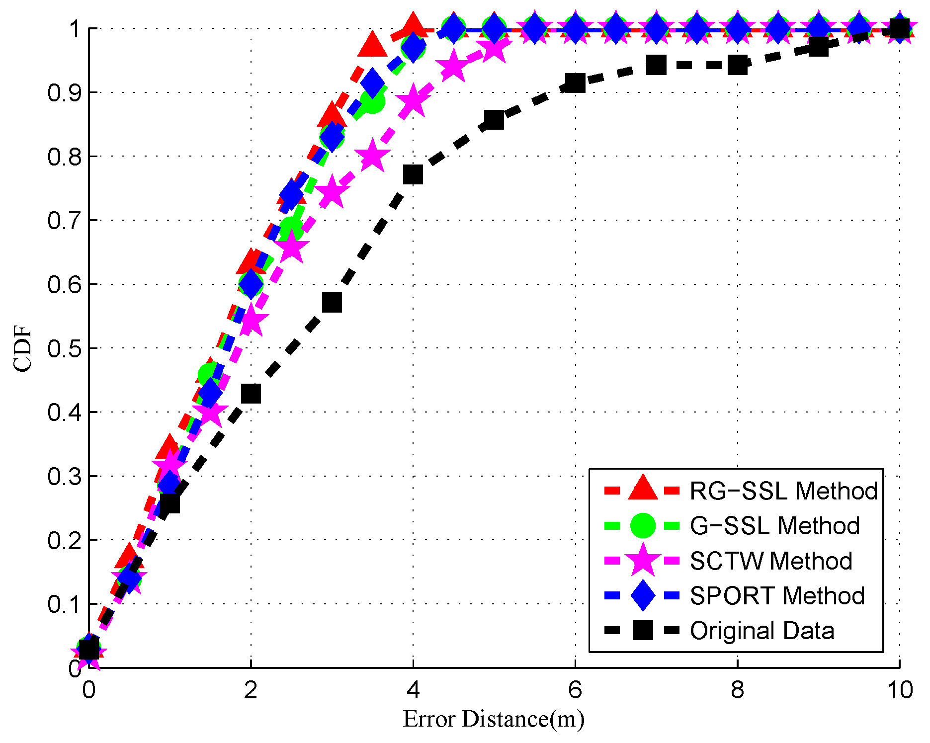
Figure 14.
Comparison of Weighted graph. (a) Weighted graph calculated by heat kernel method; (b) Weighted graph calculated by CS method.
Figure 14.
Comparison of Weighted graph. (a) Weighted graph calculated by heat kernel method; (b) Weighted graph calculated by CS method.
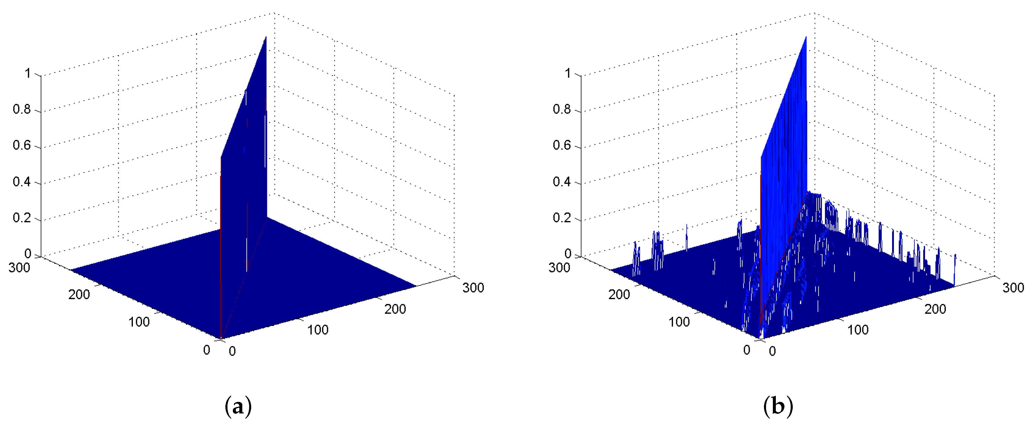
Figure 15.
Smoothed signal distribution of radio map and localization results using RSG-SSL. (a) Smoothed signal distribution of radio map; (b) Localization results.
Figure 15.
Smoothed signal distribution of radio map and localization results using RSG-SSL. (a) Smoothed signal distribution of radio map; (b) Localization results.

Figure 16.
Cumulative distribution function of localization error.


Table 1.
Comparison of different algorithms.
| Algorithm | Cumulative Probability (Location Error Is 2 m) | Average Error (m) | Maximum Error (m) |
|---|---|---|---|
| RG-SSL | 63.5% | 2.07 | 4 |
| G-SSL | 60% | 2.13 | 4.5 |
| SPORT | 60% | 2.15 | 4.5 |
| SCTW | 54.3% | 2.24 | 5.5 |
| Original data | 42.9% | 2.89 | 10 |
© 2017 by the authors. Licensee MDPI, Basel, Switzerland. This article is an open access article distributed under the terms and conditions of the Creative Commons Attribution (CC BY) license (http://creativecommons.org/licenses/by/4.0/).
Share and Cite
MDPI and ACS Style
Zhang, L.; Valaee, S.; Xu, Y.; Ma, L.; Vedadi, F. Graph-Based Semi-Supervised Learning for Indoor Localization Using Crowdsourced Data. Appl. Sci. 2017, 7, 467. https://doi.org/10.3390/app7050467
AMA Style
Zhang L, Valaee S, Xu Y, Ma L, Vedadi F. Graph-Based Semi-Supervised Learning for Indoor Localization Using Crowdsourced Data. Applied Sciences. 2017; 7(5):467. https://doi.org/10.3390/app7050467
Chicago/Turabian StyleZhang, Liye, Shahrokh Valaee, Yubin Xu, Lin Ma, and Farhang Vedadi. 2017. "Graph-Based Semi-Supervised Learning for Indoor Localization Using Crowdsourced Data" Applied Sciences 7, no. 5: 467. https://doi.org/10.3390/app7050467
Note that from the first issue of 2016, this journal uses article numbers instead of page numbers. See further details here.