Multi-Objective Climb Path Optimization for Aircraft/Engine Integration Using Particle Swarm Optimization


Propulsion Engineering Centre, School of Aerospace, Transport and Manufacturing, Cranfield University, Cranfield MK43 0AL, UK
*
Author to whom correspondence should be addressed.
Appl. Sci. 2017, 7(5), 469; https://doi.org/10.3390/app7050469
Submission received: 29 January 2017
/
Revised: 21 April 2017
/
Accepted: 26 April 2017
/
Published: 30 April 2017
(This article belongs to the Special Issue Gas Turbines Propulsion and Power)
Abstract
:In this article, a new multi-objective approach to the aircraft climb path optimization problem, based on the Particle Swarm Optimization algorithm, is introduced to be used for aircraft–engine integration studies. This considers a combination of a simulation with a traditional Energy approach, which incorporates, among others, the use of a proposed path-tracking scheme for guidance in the Altitude–Mach plane. The adoption of population-based solver serves to simplify case setup, allowing for direct interfaces between the optimizer and aircraft/engine performance codes. A two-level optimization scheme is employed and is shown to improve search performance compared to the basic PSO algorithm. The effectiveness of the proposed methodology is demonstrated in a hypothetic engine upgrade scenario for the F-4 aircraft considering the replacement of the aircraft’s J79 engine with the EJ200; a clear advantage of the EJ200-equipped configuration is unveiled, resulting, on average, in 15% faster climbs with 20% less fuel.
1. Introduction
Given the large investments required to develop new aero-engines, the costs and risks associated with such projects should be addressed as early as possible for a constructor to achieve market competitiveness and avoid the financial consequences of potentially unsuccessful designs. This is the fundamental principle that led to the introduction of the Techno-economic and Environmental Risk Assessment (TERA) software tools, which allow for management and modeling of various factors associated with a gas turbine’s operational lifecycle. The TERA concept was introduced by Cranfield University [1] and its current applications include engines for civil aviation, maritime propulsion and power generation.
Recognizing the important contribution of the propulsion system to the aircraft’s climb capabilities, in this article, a new methodology for assessing the climb performance of candidate aircraft–engine configurations is presented. This is based on a multi-objective climb path optimization search, which is used to construct Pareto fronts of solutions that minimize climb time and fuel consumption. These provide a graphical means of representing the aircraft’s climb potential and allow for comparisons between different aircraft configurations to be made.
Aircraft climb path optimization belongs to a family of trajectory optimization problems that were born out of the need to maximize the performance of air vehicles and/or reduce their operating cost and environmental impact. The pioneering work of Routowski [2] in the late 1950s may be considered as the starting point for work in this domain, later evolving to the Energy–Maneuverability Theory [3] which has contributed significantly to the quantification of aircraft performance. Though computationally inexpensive and relatively accurate, the limitations of this methodology were already evident by the late 1960s: The flyability of the optimal paths generated was not guaranteed, while simplifications associated with the method’s fundamental assumptions led, in many cases, to unavoidable deviations between actual and estimated results [4,5]. The gradual increase in the available computational resources and improvement of numerical algorithms led to the introduction of more sophisticated methods for aircraft trajectory optimization: optimal control theory and nonlinear programming have been used extensively in this scope [6,7,8,9,10]. Optimal control theory, when applied to a trajectory optimization problem, seeks an optimal control law; in other words, a sequence of control inputs that drives a given vehicle into a trajectory that minimizes a pre-defined cost function. Methods for solving optimal control problems include Dynamic Programming [11], which is restricted to small state dimensions; Indirect Methods, which use the necessary conditions of optimality to derive and numerically solve a boundary value problem; and Direct Methods, which discretize the original infinite-dimensional control problem to a finite-dimensional one and solve it using nonlinear programming techniques [12].
Genetic algorithms and, in general, population-based optimization schemes represent a more recent addition to the collection of methods for trajectory optimization [13,14,15,16,17,18,19,20]. Although the latter may not be considered computationally competitive with “traditional” optimal control methodology, they incorporate some fundamental advantages that have attracted scientific interest: The convergence of population-based methods is not affected by the smoothness or continuity of the functions being minimized; this feature is particularly suited to aerospace applications where, traditionally, tabular data are used for model construction. In the context of an aircraft–engine integration application as the one hereby considered, this does allow for a direct interface between the optimization code and the engine performance software to obtain estimates for thrust and fuel consumption, instead of resorting to simplified functional representations for the latter; in fact, when considering the detailed modeling of an aircraft powerplant, small discontinuities in these quantities and/or their derivatives are typical as a result of bleed valve, guide vane, nozzle, bleed and power extraction schedules. Furthermore, because of their very good global search capabilities and contrary to gradient-based optimization methods, population-based schemes do not require an initial guess by the user and can thus been applied to problems with solutions that are hard to estimate [15]. Combining the above with a simple and straightforward implementation leads to a significant reduction in the effort required for case setup and makes trajectory optimization accessible to users without the otherwise-necessary mathematical background or system knowledge. As a result, given the ever-increasing computational power that is available, the use of such schemes has become widespread over the last decades, replacing, in many cases, methods that are more traditional.
Yokoyama and Suzuki [15] developed a modified real-coded genetic algorithm for constrained trajectory optimization to be used for providing appropriate initial solutions to gradient-based direct trajectory optimization methods. The proposed algorithm was applied to a space vehicle’s reentry trajectory problem and produced solutions that approached the vicinity of the optimal solution. Pontani and Conway [16] applied the Particle Swarm Optimization (PSO) technique (an optimization method inspired by the social behavior of animals) to a series of space trajectory optimization cases and showed that the method is efficient, reliable and accurate in determining optimal trajectories for problems with a limited number of unknown parameters. Rahimi, Kumar and Alighanbari [17] reached the same conclusions while examining the application of PSO to spacecraft reentry trajectory optimization. Pontani, Ghosh and Conway [18] employed PSO to generate optimal multiple-burn rendezvous trajectories and used the solutions to initialize a gradient-based optimization process; good agreement between the results of the two methods was observed, demonstrating the effectiveness of the PSO scheme. Common features of all the approaches presented above are the use of a direct-shooting-equivalent problem formulation, employing parameterized curves to produce control time histories with a finite number of input variables and the implementation of constraints by means of penalty functions, selections that are dictated by the particular characteristics of the selected optimization schemes.
A rather interesting feature of population-based optimization algorithms that has recently been exploited in the field of trajectory optimization is their ability to handle multiple objectives in a single optimization run [19,20]; in a so-called multi-objective optimization case, instead of a single solution, the optimizer seeks for a set of solutions that correspond to the optimal compromises between contradicting targets; the latter form a front in the objective space, named the Pareto front. This capability partly compensates for the higher computational cost of population-based methods, since multiple runs of a comparable gradient-based optimization method are required to produce the same amount of solutions.
Considering the development of an aircraft/engine integration methodology that will address the climb performance of candidate aircraft/engine configurations, the use of a climb path optimization methodology was required, to allow for a “fair” comparison of configurations with different performance characteristics. In this context, a multi-objective formulation of the aircraft climb path optimization problem was deemed advantageous over a single-objective one because the generated Pareto fronts may better represent aircraft climb potential and allow for comparisons between different configurations to be made on a wider basis. Under this scope and given that the computational cost per simulation is rather small, a multi-objective, population-based optimization scheme was selected, also capable of being directly interfaced with the University’s engine performance software, to further simplify case setup; a user will only need to specify an engine geometry and a generic aircraft model to obtain results for the climb potential of their combination, allowing for the method to also be used for educational purposes. The authors’ intention is therefore not to present a climb path methodology that will compete with present gradient-based methods, but to introduce an easy-to-implement, non-mathematical, multi-objective formulation to the traditional climb path optimization problem to be used as a tool for aircraft–engine integration studies.
The well-tried and tested Multi-Objective Particle Swarm Optimization (MOPSO) method [21] is selected to conduct the intended multi-objective search for optimal climb paths because it combines simplicity with fine global search characteristics. Energy–Maneuverability (E-M) theory is exploited to increase the effectiveness of the search. This is achieved in two ways: Firstly, in place of producing control histories and contrary to similar methods, the optimizer uses Bezier splines to construct candidate flight paths in the form of curves in the Altitude (h)–Mach number (M) plane. Since the general form of these paths can be easily predicted by E-M, this facilitates the selection of the design parameters. To avoid limiting the optimizer’s degrees of freedom by inserting equality constraints to satisfy the aircraft state equations, a path-tracking technique for guidance in the h-M plane based on the Carrot Chasing guidance scheme [22] is introduced and used to fly an aircraft model into the designed trajectories. Secondly, a two-level optimization scheme is employed to boost convergence: An initial low-level optimization run is performed using E-M as a low-cost, low-fidelity approximate of the actual objective functions; its solutions are used to initialize a second, high-level optimization run, which employs a simulation to accurately assess the outcome of candidate flight paths. Better initialization has a positive effect on the algorithm’s convergence speed and leads to improved results for a given number of fitness function evaluations.
To demonstrate a practical application of the proposed method on a realistic aircraft–engine integration scenario, a model of the F-4 Phantom II is selected as the reference airframe for this application. This represents an aircraft type still in operational service, a fact that is combined with a wide database of aerodynamic and performance data [3,4,23,24] that have become available during the aircraft’s long operational career: On the basis of the latter, a reasonably accurate representation of the aircraft may be constructed. Throttle-dependent forces are also included to account for installation effects and allow for a more accurate integrated engine representation. Cranfield University’s in-house gas turbine performance code, Turbomatch, is used to construct engine models, outputting thrust, air mass flow, nozzle pressure ratio and specific fuel consumption. Turbomatch comprises several pre-programmed modules, which correspond to models of individual gas turbine components. They can be called up to simulate the action of the different components of the engine, resulting finally in the output of engine thrust or power, specific fuel consumption, etc. Its modularity, which is supported by the implementation of generic component maps, enables the detailed design of any gas turbine configuration. The validity of the aircraft performance model produced is assessed against published performance data [24].
The structure of this article is as follows. Section 2 presents a general description of the aircraft model, the procedure for the generation of climb paths and the proposed path tracking method. These are followed, in Section 3, by a stability analysis for the latter and an assessment of simulation results against published performance data of the aircraft. Section 4 describes the two-level optimization approach adopted and compares its performance with that of an equivalent single-level scheme. Finally, in Section 5, a test application of the developed methodology is presented, comparing the performance of the aircraft’s original J79 engine with that of the EJ200 in a hypothetical engine upgrade scenario
2. Methodology
Most studies that use population-based methods to solve optimal control problems employ parameterized curves to produce control time histories with a finite number of input variables, without exceeding the optimization algorithm’s search capabilities [15,16,17,18]. Although this approach is advantageous in terms of reducing the problem’s dimensionality, it requires some knowledge of the general shape of the time history, which, in many practical problems, can be hard to define [16]. This also applies to the aircraft climb path optimization problem, though in this case, the shape of optimal trajectories may be approximated quite well by application of E-M theory. Consequently, to exploit this information and solve the problem of solution parameterization, a direct-collocation-equivalent formulation considering the optimization of trajectories in the state domain appears to be the best approach; consistency with aircraft dynamics can be ensured by imposing equality constraints corresponding to the aircraft state equations. However, there are two fundamental difficulties associated with such a selection: Firstly, as shown by related studies [25,26], equality constraints limit the search capability of population-based optimization schemes. Secondly and most importantly, E-M solutions are trajectories in the Altitude (h)–Mach number (M) plane that cannot be directly translated to state trajectories because of the absence of the time parameter; in practice, a simulation-based approach needs to be adopted, in which an aircraft model alters between Altitude and Mach number-based guidance logic to fly into a particular trajectory [4]. Switching between the two guidance laws is case-dependent and needs to be programmed by hand, rendering it unsuitable for an optimization application.
Considering the above, in this article, a simulation-based optimization approach is proposed, in which the optimizer seeks for optimal trajectories in the h-M plane and uses Bezier splines to form candidate solutions. The latter are evaluated by means of an aircraft model which is flown into the designed trajectories using a proposed path-tracking scheme for “automated” guidance in the h-M plane. A complete description of the proposed methodology is given in the following sub-sections.
2.1. Aircraft Model
An aircraft state-space model [27] was developed and used as a platform to assess the performance of candidate trajectories. In order to cut down on the simulation’s computational intensity, the simplest possible representation was selected, comprising only four states , directly related to the intended climb performance studies. The resulting model can be generically described as a single-Degree-of-Freedom (DOF) navigation, two-DOF point mass aircraft state-space model, augmented with a mass state so as to account for engine fuel burn. The exact formulas for the aircraft state equations are given in Equations (1)–(6), expressed with respect to an earth coordinate system.
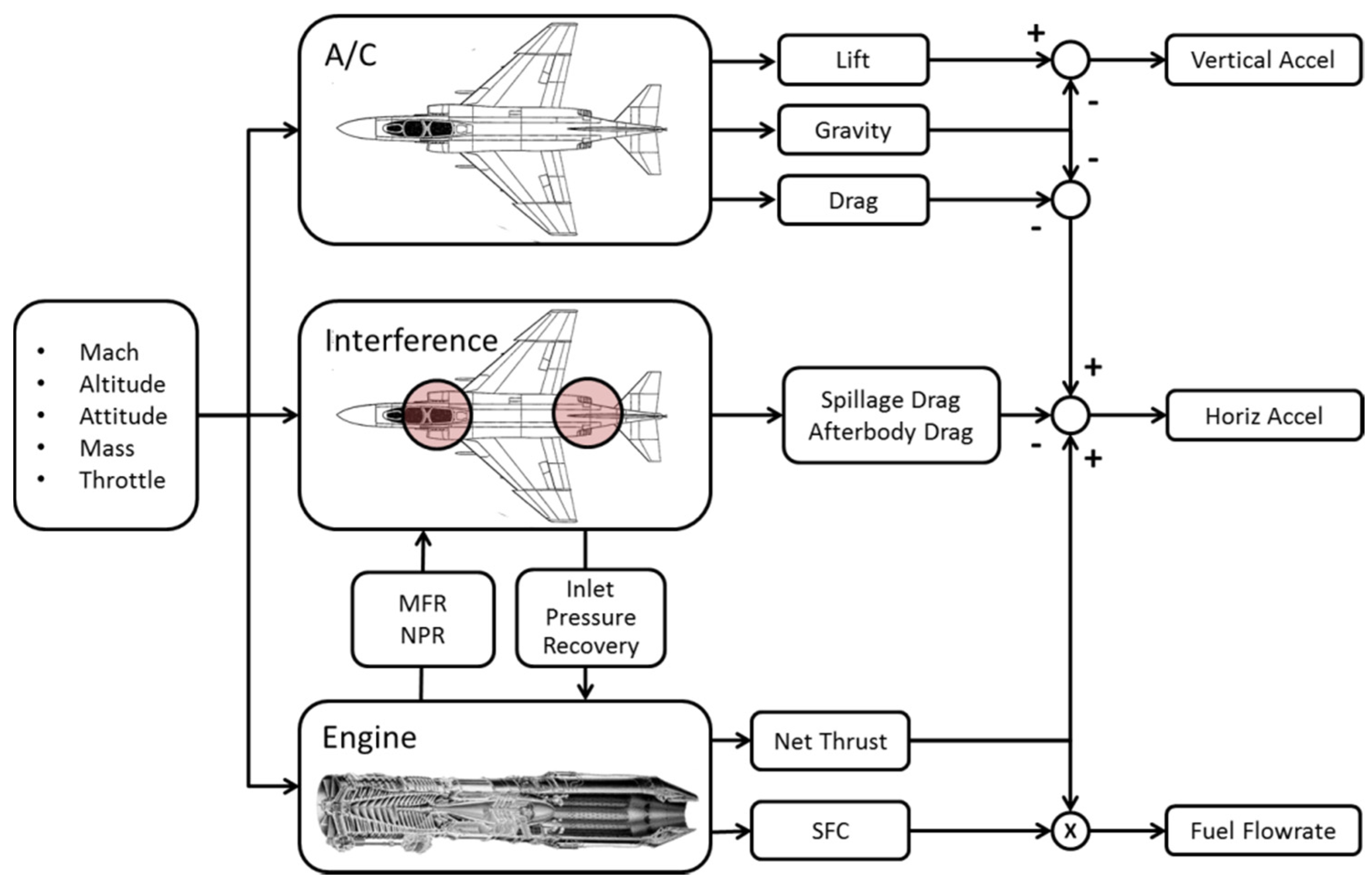
Modeling was based upon published aerodynamic and mass data for the F-4 aircraft [23,24], combined with Cranfield University’s in-house gas turbine performance code, Turbomatch, which was used to construct models for the aircraft’s engines, outputting Thrust (T), air Mass Flow (MF), Nozzle Pressure Ratio (NPR) and Specific Fuel Consumption (SFC). Turbomatch is a software based Gas Turbine performance simulation tool developed by the Propulsion Engineering Centre at Cranfield University [28]. The tool is a 0-D performance simulation code, featuring OD and transient simulation as well [29]. Turbomatch comprises several pre-programmed modules, which correspond to thermodynamic models of components. They are called up to evaluate the engine output, i.e., thrust or power, specific fuel consumption, etc. Its modularity, which is supported by the implementation of generic component maps, enables the detailed design of any gas turbine configuration. Inlet pressure recovery was modeled as a function of Mach number, as per MIL-E-5007D [30]. Throttle-dependent forces were also included to account for installation effects: The experimental data of References [31,32] were used to construct surrogate models for spillage and afterbody drag respectively. A schematic representation of the general model arrangement is depicted in Figure 1.
For the simulation runs, a constant throttle setting was assumed, in accordance with standard practice in aircraft climb sequences [24,33]. A variable-throttle approach (one that considers the sequence of throttle inputs as a problem variable), as adopted in other studies, would be computationally demanding for the detailed engine representation required for aircraft–engine integration applications, since engine transient response would need to be modeled and is anyway impractical for a real-world scenario, being too complicated to be executed by a human pilot. Flight path angle control was used to control the aircraft’s climb rate and airspeed to fly commanded paths in the Pressure Altitude (h)–Mach Number (M) plane. The exact guidance logic employed is addressed in Section 2.3. Flight path angle rate saturation was implemented to the model to represent the aircraft’s maximum lift capability and structural strength (Equations (3) and (5))
2.2. Generation of Climb Paths
To exploit the fact that the general form of optimal trajectories in the h-M plane can be estimated using E-M theory, in the present study, Bezier splines [34] were selected for the generation of climb paths in the form of two-dimensional curves in this plane. These are parametric curves built around polynomial expressions, known as the Bernstein polynomials. A Bezier curve of order n is defined by a set of control points, through , under the formula:
The selection of Bezier splines to construct flight paths is justified by a number of advantages over other curve-fitting approaches:
- Complex curve geometries may be generated using a small number of control variables.
- Boundary conditions may be easily applied.
- Bezier splines allow for the representation of non-functional relations between h and M, which may be generated by combinations of accelerated climbs/descents with zoom climb-type maneuvers.
- The curves produced are directional, a feature that can be exploited by the aircraft’s path-tracking guidance logic.
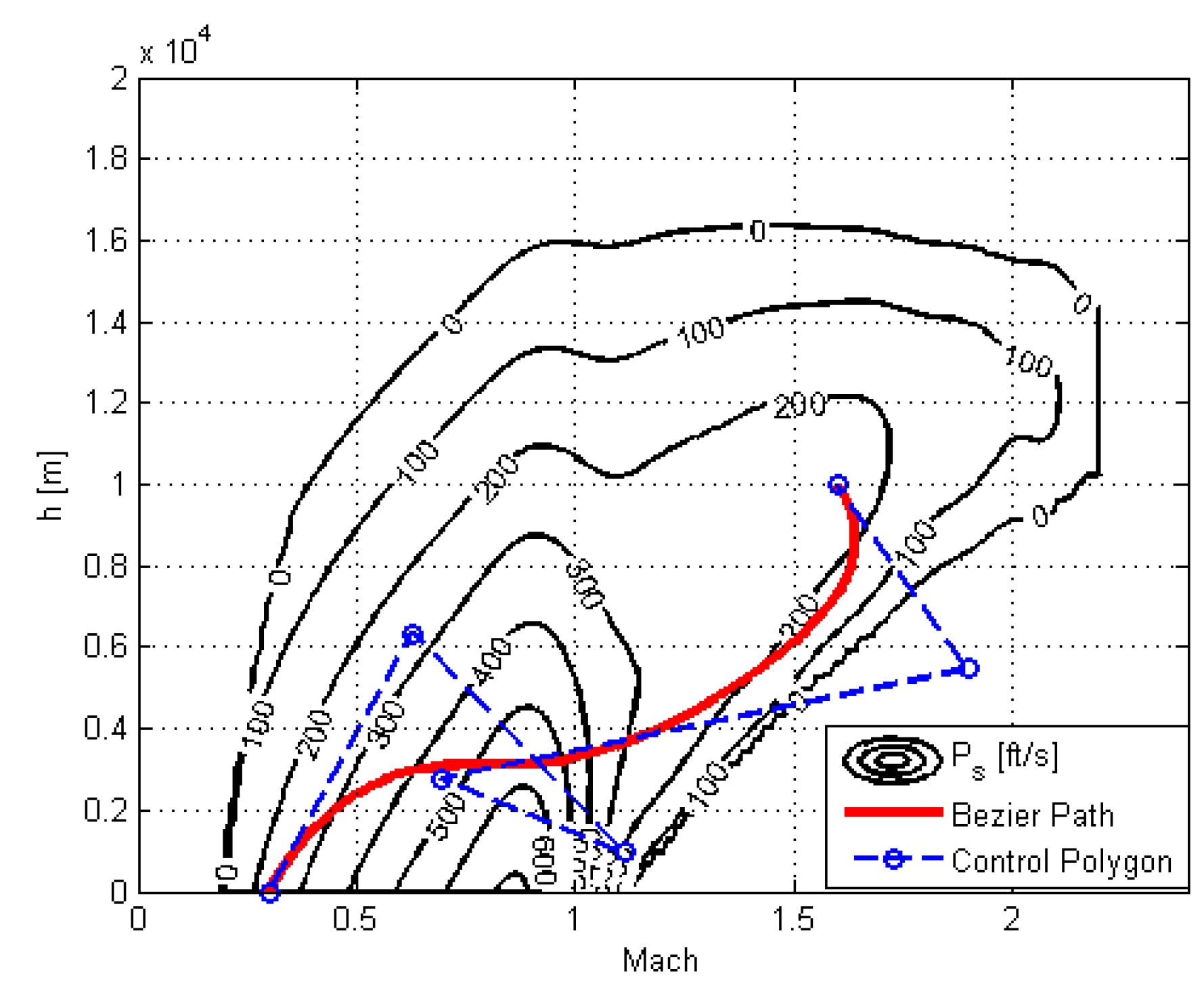
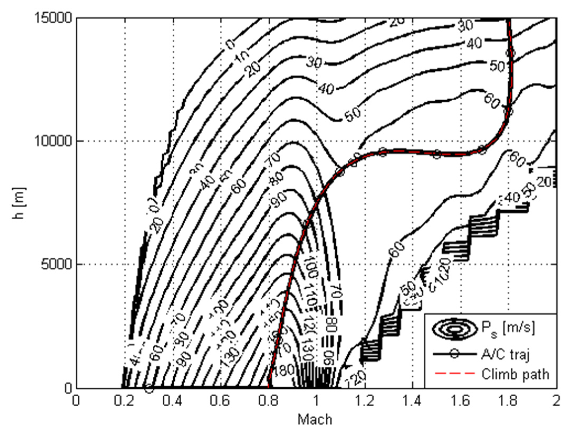
An example of a Bezier-spline-generated climb path is shown in Figure 2, plotted over contours of Specific Excess Power.
An acceptable climb path should have positive values of altitude along its entire length; depending on the splines’ degrees of freedom, this may lead to an excessive number of rejected (or penalized) solutions during the optimization run. With a view to reducing the amount of unacceptable solutions without affecting the optimizer’s performance, in place of an inequality path constraint, the resulting negative values were simply forced to zero. Hence,
2.3. Guidance
2.3.1. Aircraft Control
Assuming a constant throttle setting, the aircraft’s rate of climb and airspeed may be simultaneously controlled by properly adjusting its flight path angle. From the definitions of Specific Energy () and Specific Excess Power () [3]:
Using the chain rule:
Combining Equations (11) and (12),
Knowing that , Equation (13) becomes:
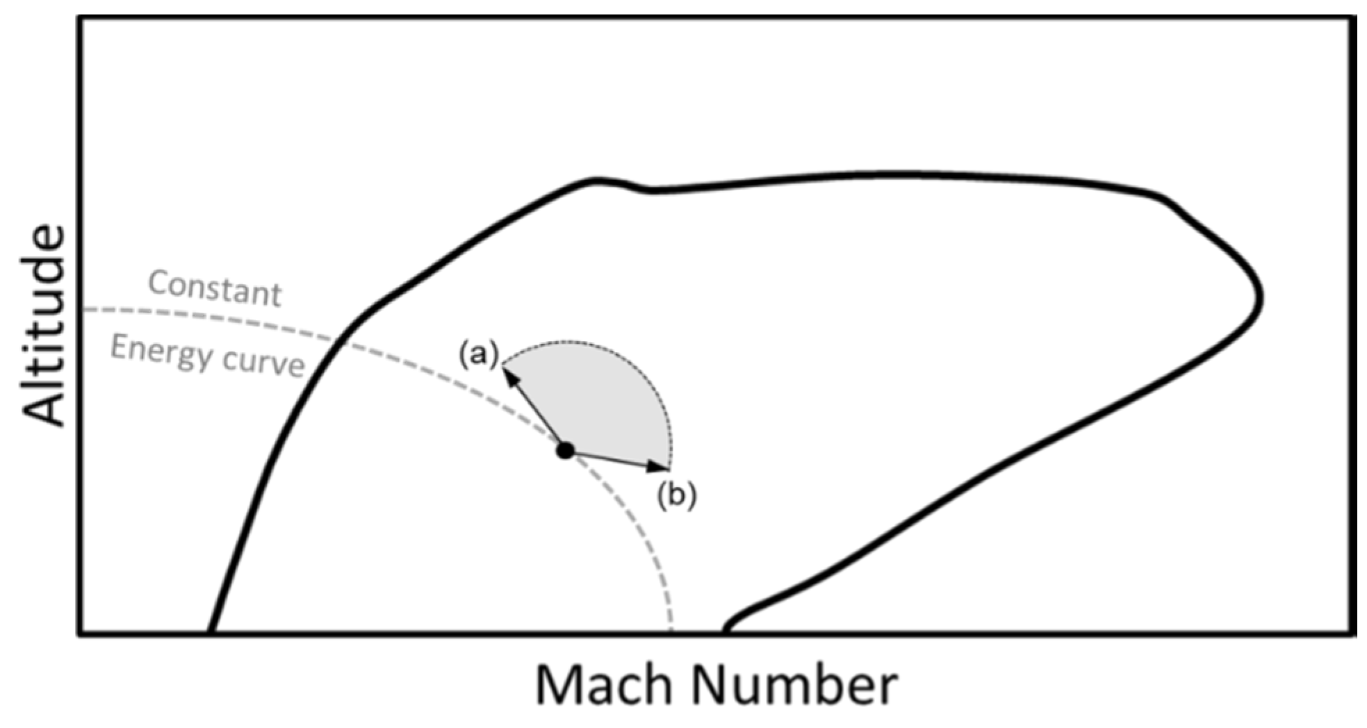
It is thus possible to fly in a particular direction in the H-M plane only by controlling the aircraft’s flight path angle. Limitations, however, do exist:
For :
The limiting value corresponds to the aircraft climbing vertically.
Equivalently, for :
the limiting value corresponding to a vertical dive.
Both limitations are presented graphically in Figure 3, the shaded area denoting the range of physically possible transitions in the h-M plane.
2.3.2. Path Tracking
In order to evaluate the specified climb paths, a non-linear path-tracking guidance method was developed and used to guide the aircraft model in the h-M space. This was inspired by the Carrot Chasing algorithm [22], adapted to match the particular characteristics of the examined guidance problem.
From the derivation of the previous sub-section, it was shown that, subject to some limitations, it is possible to fly in a particular direction in the h-M plane by properly adjusting the aircraft’s flight path angle. Hence, a transition from an initial state (0) to new state (1) can be realized by setting the flight path angle to a value so that , being the angle formed between the states’ relative position vector and the M axis (Figure 4). Consequently, instead of controlling the rate of rotation of the vehicle’s velocity vector, as in typical guidance applications, direct control over the direction of displacement in the h-M plane is available. Based on this feature and the Carrot Chasing guidance scheme, a methodology for path tracking in the h-M plane was developed. This is presented schematically in Figure 5.
Let C represent an arbitrary curve in the h-M plane, the vehicle’s current position and the projection of on C. A reference point is generated on C, at a distance downstream of . The direction of the vehicle’s displacement vector is defined as:
Point is equivalent to the Virtual Target Point used in the Carrot Chasing path tracking algorithm and is generated by means of numerical integration over curve C so as to appear at a fixed curve length downstream of .
The path tracking methodology hereby presented was evaluated over a wide variety of flight paths, displaying very good overall performance in following the specified trajectories (Figure 6).
3. Validation
3.1. Stability Analysis of the Proposed Path Tracking Method
In this Section, a study of the stability characteristics of the proposed path-tracking method is conducted over a circular trajectory of radius R. Results may be generalized for any curve C by setting R equal to the local curvature of C. In order to focus on the performance of the path-tracking algorithm aircraft dynamics have been neglected; it is hereby assumed that the aircraft reproduces all commands instantaneously and without error. Figure 7 illustrates the system geometry for the examined case.
For a path with fixed curvature:
Consequently,
The rate of change of cross-track error equals
From the triangle :
From Equations (20) and (21), knowing that , are constant:
which is the system’s state-space model. For equilibrium, the system’s state vector must remain invariable. Consequently:
Combining Equations (19), (21) and (23) yields
which corresponds to a point inside the circle where becomes normal to , as shown in Figure 7.
Some steady-state cross-track error is thus unavoidable, given that a positive value of is required for path-tracking; this, however, may become negligible if angle is set at an adequately small value, i.e., .
Angle is bounded in the interval , consequently, from Equations (19) and (21), is also bounded:
From Equation (22), f is monotonous for , as a synthesis of monotonous functions:
Let , and a Lyapunov-candidate function . Then:
Using Equation (26)
Therefore, is asymptotically stable for all possible values of .
3.2. Aircraft Model Validation
As for any performance model, an assessment of its outputs was required in order to check the validity of the produced predictions. Performance data from the aircraft’s operating manual [24] were used under this scope: The optimal climb sequences listed in the latter for both maximum and military power settings were simulated and results were compared with the respective data for an aircraft AUM of 18,000 kg.
Figure 8 shows the trajectories followed during the two simulation runs. Results for Time To Climb (TTC) and Fuel To Climb (FTC) are compared with the respective estimates from the flight manual in Table 1 and Table 2. In both cases, the level of agreement achieved (average RMS error was 2.987%) was deemed sufficient for the intended application of the model.
4. Optimization Approach
4.1. Multi-Objective Particle Swarm Optimization (MOPSO)
Particle Swarm Optimization (PSO), first introduced in [35], accounts for a population-based optimization algorithm inspired by the social behavior of animals. The baseline PSO algorithm combines simplicity with fine search capabilities: A population (swarm) of n particles is initialized at random positions within a search space of dimension D, assigned with random velocities . At the end of each step of the PSO algorithm, positions of all particles are updated, using the following set of equations:
For particle i, step j and search variable k:
where stands for the position of the global best, namely, the best-so-far solution discovered by the swarm; stands for the position of the particle’s personal best which represents the best-so-far solution discovered by the particle itself; are constants (named social factor, cognitive factor and inertia weight respectively); , are random numbers uniformly distributed in [0,1]; k = 1,…, D where D is the number of search variables.
As with most similar algorithms, a variety of multi-objective variants of PSO have been proposed expanding the method’s capabilities to handle multiple objectives in a single optimization run [36]. Among these, the Multi-Objective Particle Swarm Optimization (MOPSO) introduced in [21] represents one of the most popular approaches and has been adopted for this study. The method retains the basic features of PSO, its principal difference with the latter lying in the selection of the global best: Instead of a single position in search space, the global best is chosen from an external repository containing the members of the updated Pareto front by means of a roulette wheel selection scheme weighted in accordance with the local density of the front. The procedure comprises the following steps:
- 5.
- The objective space is divided into hypercubes and the number of non-dominated solutions contained into each hypercube is calculated.
- 6.
- Each non-empty hypercube is assigned with a fitness values inversely proportional to the number of non-dominated solutions it contains, through the formula:
- 7.
- Using fitness values , a roulette wheel selection is conducted to select the hypercube from which the global best will be taken. The probability of hypercube being selected is:
- 8.
- The global best position is picked at random from the solutions contained within the chosen hypercube.
4.2. Two-Level PSO-Based Approach to Aircraft Climb Path Optimization
Criticism over population-based optimization methods mainly focuses on the excessive number of fitness function evaluations required for locating the optimal solutions: Although these methods are very capable of conducting a global search in the optimization domain, in applications where the computational cost per evaluation is considerable, the optimization turnaround time becomes excessive. For a preset number of fitness function evaluations, in some cases this results in sub-optimal, non-converged solutions. To remedy this problem, two options are generally available:
- A reduction in the number of design variables.
In this article, in order to introduce a computationally competitive climb path optimization methodology, both strategies were adopted: As specified in Section 2, Bezier splines were used for the generation of climb paths, reducing design variables to the coordinates of a finite number of control points, rather than solving the original highly dimensional optimal control problem; the use of a parameterized curve is a common feature with other, similar methods, however, these are hereby used to design trajectories and not control sequences, facilitating the selection of inputs. Furthermore, E-M predictions are used as a surrogate model of the actual cost functions in a proposed two-level optimization strategy. This focuses on reducing the turnaround time of the simulation-based optimization run by pre-evaluating the problem in the E-M domain: An initial low-level optimization run is performed using E-M as a low-cost, low-fidelity approximate of the actual objective functions. TTC and FTC are obtained from numerical integration of the quantities:
along candidate flight paths, accounting for fuel flow rate.
Whereas “traditional” E-M considers trajectory optimization only in terms of time and fuel burn, it is evident that a simple modification of Equation (33) (in particular, a replacement of with another appropriate measure) can be used to generate cost functions for other quantities that have recently attracted scientific interest, such as noise and pollutant emissions. For reasons of simplicity, in the present study, however, the analysis is restricted to minimum time and fuel trajectories, which are more suited to the military aircraft/engine integration application that is presented.
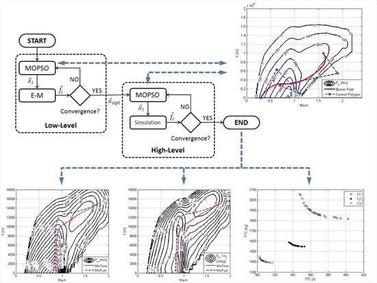
Solutions generated at the first level are used to initialize a second, high-level optimization run which employs the aircraft simulation to accurately assess the outcome of candidate flight paths. In both levels, the MOPSO algorithm is used to conduct the search. The flowchart of the process is shown in Figure 9.
The performance of the two-level optimization scheme was compared with that of standard MOPSO in a climb path optimization problem with 8 design variables (4 control points × 2 coordinates per point) using a population of 20 particles. After some trial and error analysis, PSO constants were set at and . For the two-level optimization case, an initial low-level run of 300 iterations was specified. Start conditions were set at M = 0.8, h = 0 m and end conditions at M = 1.8, h = 14,000 m. The hypervolume indicator [39] was used to compare the convergence speed of the two methods. In a two-objective problem, this equals the area of the objective space formed between the origin and a user-defined “nadir” point (for our study, this was set at (800, 2500)) that is dominated by the Pareto front.
In order to address the randomness of the PSO, 10 optimization runs were performed for each method. The averaged convergence histories are shown in Figure 10 and the mean and standard deviation values of the final solutions are included in Table 3. These indicate that the proposed approach displayed consistently faster convergence over the basic MOPSO method, which is initialized using a homogeneous random distribution of the particles in the design space. As expected, the injected optimal solutions from the E-M calculations were sub-optimal when evaluated by means of the aircraft simulation; the average hypervolume of the injected front was rather low when compared to the converged solutions and was equaled by MOPSO after only a few iterations. Despite this, the large number of well-placed solutions that were injected to the initial population did consistently boost convergence speed, leading to better fronts for a given amount of fitness function evaluations (Figure 11).
5. Application
As an example application of the proposed methodology, a hypothetical engine upgrade scenario is examined. This considers a replacement of the aircraft’s original J79 turbojet engine with the EJ200 low-bypass turbofan, which has a similar design air mass flow rate.
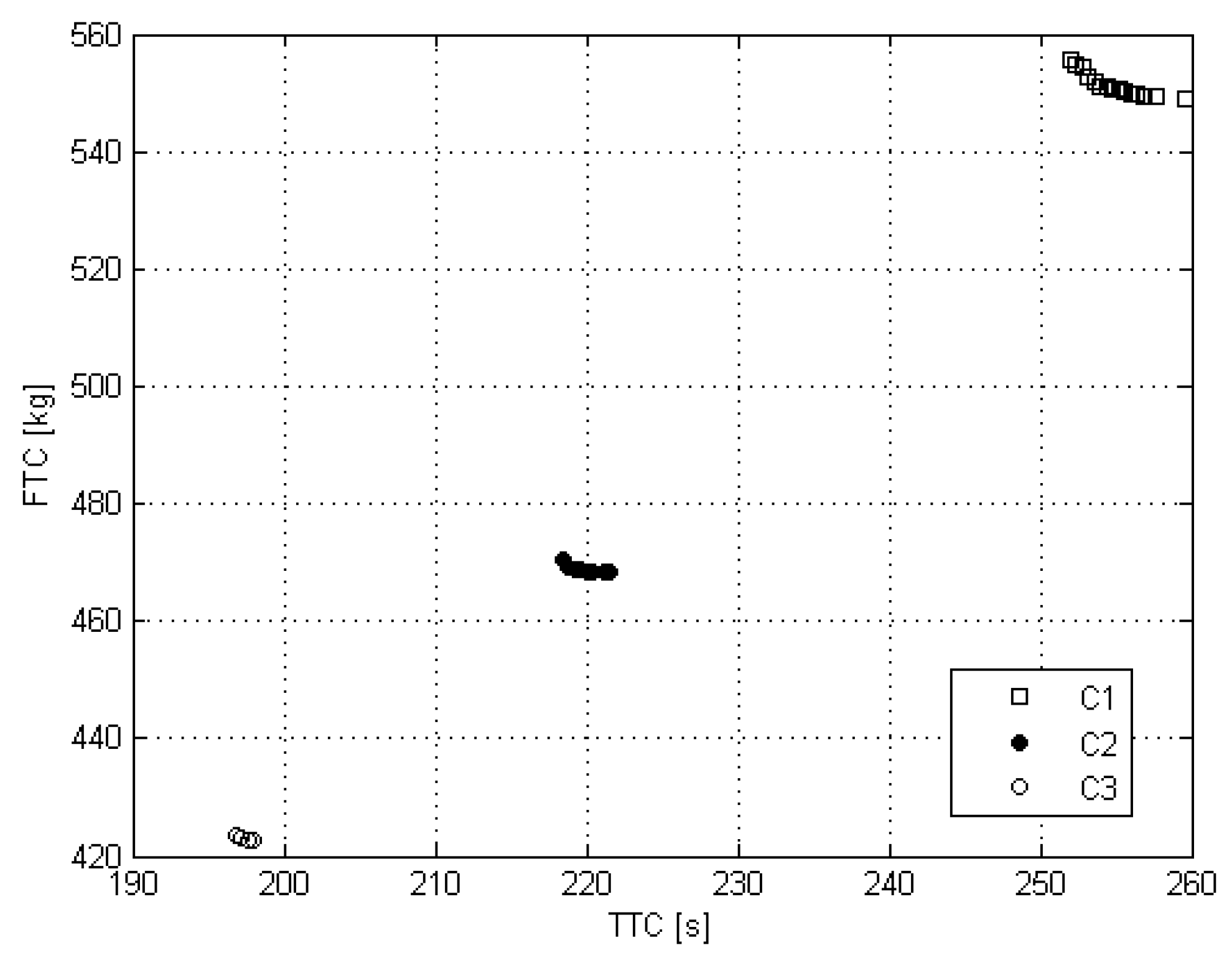
Under this scope, the climb performance of three aircraft–engine configurations is examined using the proposed multi-objective climb path optimization methodology. A summary of their specifications is given in Table 4. Configuration C1 is the original aircraft configuration, while configurations C2 and C3 correspond to EJ200-equipped variants. Configuration C2 shares the same AUM with configuration C1, assuming that, as a result of the reduced weight of the EJ200 engines, the airframe’s weight is allowed to increase with the addition of extra equipment or internal fuel. Configuration C3 shares the shame airframe and internal fuel weight with Configuration C1, resulting in a reduced aircraft AUM.
To assess the performance of the above configurations, two test cases are evaluated, their details being provided in Table 5. Case A examines a typical subsonic mission climb scenario, where an aircraft, after takeoff, uses a military (maximum, non-afterburning) thrust setting to climb to the optimum cruise altitude. Case B, on the other hand, considers a maximum power supersonic climb, to be encountered in a supersonic, point-intercept-type mission.
A population of 20 particles was selected and run for 300 low-level and 100 high-level iterations in all test cases. Four control points were employed for the test runs of Case A and six for the runs of Case B, corresponding to eight and twelve design variables, respectively. In both cases, PSO constants were set at and . Results are presented in Figure 12, Figure 13, Figure 14 and Figure 15 for Case A and Figure 16, Figure 17, Figure 18 and Figure 19 for Case B. For reasons of clarity, only flight paths corresponding to minimum-time and minimum-fuel solutions are shown, intermediate flight paths being bounded within them.
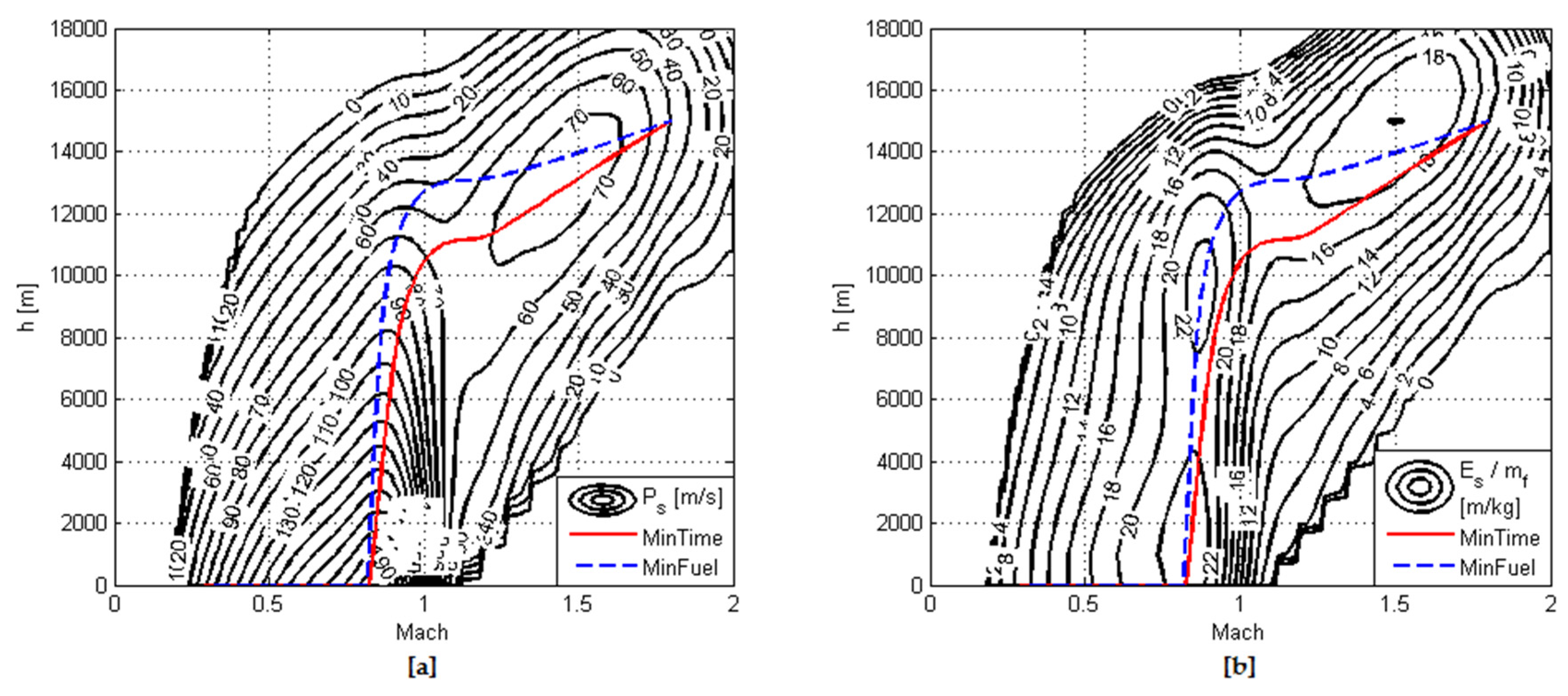
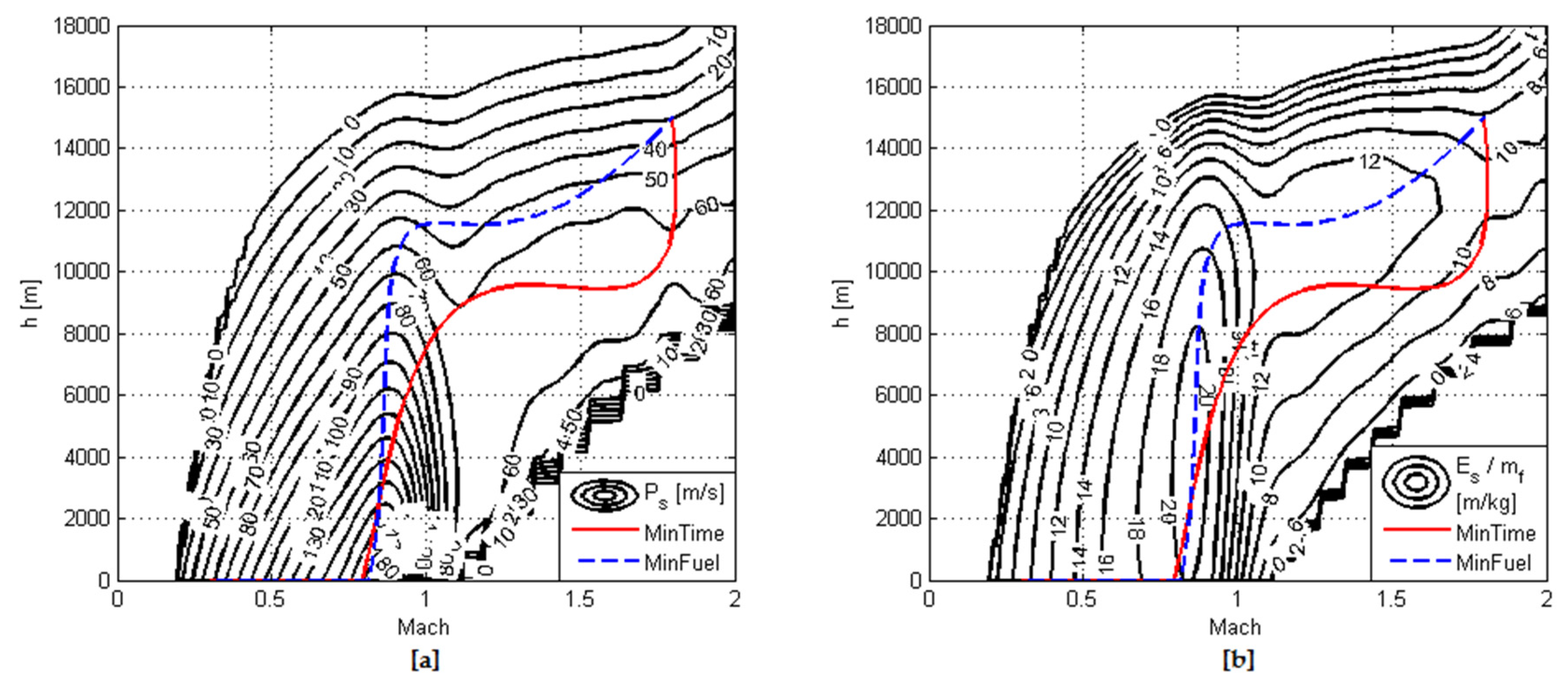
A qualitative assessment of the resulting trajectories indicates that these are in agreement with related theoretical estimates and published results [2,3,4,5,9]: All paths begin with a level acceleration at sea level where the aircraft has its maximum acceleration capability. In the subsonic climb case, this is followed by an accelerated climb that follows the peaks of the Specific Excess Power (for the minimum-time climb) and Energy Efficiency (for the minimum-fuel climb) contours up to the specified end conditions; this is a good indication for the accuracy of the generated solutions, since the optimizer, by definition, uses no information about the gradients of the respective functions. In the supersonic climb case, the tracking of contours usually results in a dive occurring in the transonic region. In minimum-fuel climb paths, climbs begin at lower subsonic Mach numbers than in the respective minimum time paths, trajectories being shifted towards higher altitudes for improved efficiency. In general, in all cases and in accordance with the results of Reference [4], the resulting paths look like “smoothed” versions of E-M paths. This is because E-M solutions do not take into account the energy loss during maneuvers and assume that the transition between equal energy levels may be realized instantaneously; if the latter are considered, climb path optimization becomes a tradeoff between accurate tracking of contours and avoidance of intense maneuvers.
As far as the performance of the examined configurations is concerned; an inspection of Figure 12 and Figure 16 denotes a clear advantage of the EJ200-equipped configurations. In the subsonic climb case; an average 14.5% reduction in fuel consumption was combined with 13.7% reduction in time to climb with respect to the aircraft’s original configuration at an equal aircraft AUM (Configuration C2). The above values were further increased to 23.6% and 22.7%, respectively, if the weight reduction resulting from the reduced engine weight were considered (Configuration C3). A similar picture was observed in the supersonic climb test results: The average reduction in fuel consumption was 17.3% for configuration C2 and 25.3% for configuration C3 accompanied by a 6.7% and 18.9% reduction in climb time, respectively.
A comparison of the maximum power Specific Excess Power and Energy Efficiency contours of the three examined configurations unveils the different performance characteristics of the engines examined: The EJ200 is a low-bypass turbofan engine with a higher static thrust than the J79 turbojet. This accounts for an acceleration and efficiency advantage of the former over most of the aircraft’s envelope, particularly at high altitude and low-to-medium Mach numbers. On the contrary, because of its turbojet cycle, the J79 has better performance at medium altitudes in the transonic Mach number range, gradually expanding to the entire altitude range as the Mach number further increases. In Case B, this results in smaller differences in TTC between configuration C1 and configurations C2 and C3 compared to the results of Case A (Figure 12 and Figure 16). The different performance characteristics of the two engines also become evident by comparing the minimum-time supersonic climb trajectories of configurations C2 and C3 with that of configuration C1. The J79-equipped configuration (C1) favors an acceleration at medium altitude in the transonic regime, followed by a zoom climb to reach the specified altitude (Figure 17), whereas the EJ200-equipped configurations (C2 and C3) use a subsonic climb to high altitude followed by an accelerated supersonic climb to the desired conditions (Figure 18 and Figure 19). On the contrary, minimum-fuel supersonic climb trajectories are similar for both engines, which lead to a rather “broad” front of optimal solutions for configuration C1 (Figure 16) compared to the respective results for configurations C2 and C3. The same, to a smaller degree, also apply to the results of the subsonic climb case, as may be observed in Figure 12, Figure 13, Figure 14 and Figure 15: The greater “distance” between minimum-fuel and minimum-time trajectories for configuration C1 leads to greater variations in FTC and TTC among members of the resulting front. Consequently, this constitutes an additional advantage of the EJ200-equipped configurations since the relative coincidence between minimum-time and minimum-fuel climb paths minimizes the compromises required (in fuel when climbing for the minimum time and the reverse) in each climb case. As a general conclusion, the characteristics of the low-bypass turbofan cycle appear to be better suited to typical aircraft mission requirements, leading to faster climbs with less fuel consumption. On the other hand, the regions where the performance of the turbojet is dominant are of little operational interest, a fact that is justified by the evolution of military aircraft engines since the development of the J79 in the late 1950s.
6. Conclusions
Population-based schemes represent a rather recent addiction to the collection of methods for aircraft trajectory optimization that, despite their rather high computational cost, combine extreme simplicity with robustness and are therefore accessible to a larger number of users. In this article, the authors considered the development of an easy-to-implement, non-mathematical, multi-objective formulation to the traditional climb path optimization problem to be used as a tool for aircraft–engine integration studies. This was built upon a combination of a simulation-based optimization scheme using the Multi-Objective Particle Swarm Optimization method with “traditional” Energy–Maneuverability theory. The combination of the two methods was shown to output better results than any of the methods individually.
As part of the proposed optimization methodology, and to avoid inserting equality constrained that would limit the optimizer’s search capability, a new variant of the Carrot Chasing guidance method was introduced and used to guide the aircraft model through specified trajectories in the Altitude (h)–Mach (M) plane. Tested on a wide variety of possible trajectories, the proposed guidance method was found to produce very accurate path tracking.
The performance of the developed methodology was demonstrated in a test application, which compared the performance of J79- and EJ200-equipped variants of an F-4-like aircraft, in a hypothetical engine upgrade scenario. Pareto fronts of solutions that minimize climb time and fuel consumption were generated using the proposed optimization scheme and used to compare the performance of the different aircraft/engine configurations. Results denoted a clear advantage of the EJ200-equipped configurations in both subsonic and supersonic climb conditions: on average, 15% faster climbs were achieved with 20% less fuel consumption. As expected, the characteristics of the low-bypass turbofan cycle were found to be better suited to aircraft mission requirements, while the regions where the performance of the turbojet was dominant were of little operational interest; a point that is justified by the evolution of military aircraft engines since the development of the J79.
As a concluding remark, it is important to note that, if an actual engine replacement for an F-4 fleet were to be examined, various other factors would need to be considered, such as the costs for engine purchase and airframe modification, the overall gain in mission performance and the fleet’s remaining operational life. Such issues are out of the scopes of the presented methodology and will be addressed in future studies by the authors, as part of the synthesis of a TERA module for military aircraft applications.
Author Contributions
Aristeidis Antonakis and Pericles Pilidis developed the optimization methodology, conceived and designed the experiments; Aristeidis Antonakis created the aircraft performance model and performed the experiments; Theoklis Nikolaidis created the engine performance models, reviewed and analyzed the data; Aristeidis Antonakis drafted the paper; Pericles Pilidis and Theoklis Nikolaidis reviewed the draft paper and added changes for final publication.
Conflicts of Interest
The authors declare no conflict of interest.
Nomenclature
| a | speed of sound |
| AUM | All-Up Mass |
| c | commanded |
| CD0 | zero-lift drag coefficient |
| CL | lift coefficient |
| D | drag |
| DOF | Degrees Of Freedom |
| Es | specific energy |
| E-M | Energy–Maneuverability |
| FTC | Fuel To Climb |
| g | gravitational acceleration |
| h | altitude |
| k | induced drag coefficient |
| L | lift |
| M | Mach number |
| m | mass |
| nz | load factor |
| Ps | specific excess power |
| S | wing area |
| SFC | Specific Fuel Consumption |
| T | thrust |
| TTC | Time To Climb |
| V | velocity |
| γ | flight path angle |
| ρ | air density |
| τ | time constant |
References
- Ogaji, S.; Pilidis, P.; Hales, R. TERA—A Tool for Aero-engine Modelling and Management. In Proceedings of the 2nd World Congress on Engineering Asset Management and the 4th International Conference on Condition Monitoring, Harrogate, UK, 11–14 June 2007. [Google Scholar]
- Rutowski, E. Energy Approach to the General Aircraft Performance Problem. J. Aeronaut. Sci. 1954, 21, 187–195. [Google Scholar] [CrossRef]
- Boyd, J.; Christie, T.; Gibson, J. Energy-Maneuverability; AD372287; Eglin AFB: Valparaiso, FL, USA, 1966. [Google Scholar]
- Johnson, D. Evaluation of Energy Maneuverability Procedures in Aircraft Flight Path Optimization and Performance Estimation; AD754909; Wright Patterson Air Force Base: Dayton, OH, USA, 1972. [Google Scholar]
- Takahashi, T. Optimal Climb Trajectories through Explicit Simulation. In Proceedings of the 15th AIAA Aviation Technology, Integration and Operations Conference, Dallas, TX, USA, 22–26 June 2015. [Google Scholar]
- Betts, J. A Survey of Numerical Methods for Trajectory Optimization. J. Guid. Control Dyn. 1998, 21, 193–207. [Google Scholar] [CrossRef]
- Ong, S. Sequential Quadratic Programming Solutions to Related Aircraft Trajectory Optimization Problems. Ph.D. Thesis, Iowa State University, Ames, IA, USA, 1992. [Google Scholar]
- Chircop, K.; Zammit-Mangion, D.; Sabatini, R. Bi-Objective Pseudospectral Optimal Control Techniques for Aircraft Trajectory Optimization. In Proceedings of the 28th International Congress of the Aeronautical Sciences, Brisbane, Australia, 23–28 September 2012. [Google Scholar]
- Pierson, B.; Ong, S. Minimum-Fuel Aircraft Transition Trajectories. Math. Comput. Model. Int. J. 1989, 12, 925–934. [Google Scholar] [CrossRef]
- Karelahti, J.; Virtanen, K. Automated Solution of Realistic Near-Optimal Aircraft Trajectories using Computational Optimal Control and Inverse Simulation. In Proceedings of the AIAA Guidance, Navigation and Control Conference and Exhibit, Hilton Head, SC, USA, 20–23 August 2007. [Google Scholar]
- Bertsekas, D. Dynamic Programming and Optimal Control; Athena Scientific: Belmont, MA, USA, 1995; Volume 1. [Google Scholar]
- Von Stryk, O.; Bulirsch, R. Direct and Indiret Methods for Trajectory Optimization. Ann. Oper. Res. 1995, 37, 357–373. [Google Scholar] [CrossRef]
- Holub, J.; Foo, J.; Kilivarapu, V.; Winer, E. Three Dimensional Multi-Objective UAV Path Planning using Digital Pheromone Particle Swarm Optimization. In Proceedings of the 53rd AIAA/ASME/ASCE/AHS/ASC Structures, Structural Dynamics and Materials Conference, Honolulu, HI, USA, 23–26 April 2012. [Google Scholar]
- Bower, G.; Kroo, I. Multi-Objective Aircraft Optimization for Minimum Cost and Emissions over Specific Route Networks. In Proceedings of the 26th International Congress of the Aeronautical Sciences, Anchorage, AK, USA, 14–19 September 2008. [Google Scholar]
- Yokoyama, N.; Suzuki, S. Modified Genetic Algorithm for Constrained Trajectory Optimization. J. Guid. Control Dyn. 2005, 28, 139–144. [Google Scholar] [CrossRef]
- Pontani, M.; Conway, B. Particle Swarm Optimization applied to Space Trajectories. J. Guid. Control Dyn. 2010, 33, 1429–1441. [Google Scholar] [CrossRef]
- Rahimi, A.; Kumar, K.D.; Alighanbari, H. Particle Swarm Optimization applied to Spacecraft Reentry Trajectory. J. Guid. Control Dyn. 2013, 36, 307–310. [Google Scholar] [CrossRef]
- Pontani, M.; Ghosh, P.; Conway, B. Particle Swarm Optimization of Multiple-Burn Rendezvous Trajectories. J. Guid. Control Dyn. 2012, 35, 11192–11207. [Google Scholar] [CrossRef]
- Othman, N.; Kanazaki, M. Development of Multiobjective Trajectory-Optimization Method and its Application to Improve Aircraft Landing. Aerosp. Sci. Technol. 2016, 58, 166–177. [Google Scholar] [CrossRef]
- Vavrina, M.; Howell, K. Multiobjective Optimization of Low-Thrust Trajectories Using a Genetic Algorithm Hybrid. In Proceedings of the AAS/AIAA Space Flight Mechanics Meeting, Pittsburgh, PA, USA, 9–13 August 2009. [Google Scholar]
- Coello, C.; Lechunga, M. MOPSO: A proposal for multiple objective particle swarm optimization. In Proceedings of the 2002 Congess on Evolutionary Computation, part of the 2002 IEEE World Congress on Computational Intelligence, Honolulu, HI, USA, 12–17 May 2002. [Google Scholar]
- Sujit, P.; Saripalli, S.; Sousa, J. An Evaluation of UAV Path Following Algorithms. In Proceedings of the 2013 European Control Conference, Zurich, Switzerland, 17–19 July 2013. [Google Scholar]
- Heffley, R.; Wayne, F. Aircraft Handling Qualities Data; NASA CR-2144; NASA: Washington, DC, USA, 1972.
- US Department of the Navy. NATOPS Flight Manual Navy Model RF-4B Aircraft; US Department of the Navy: Washington, DC, USA, 1965.
- Hu, X.; Eberhart, R. Solving Constrained Nonlinear Optimization Problems with Particle Swarm Optimization. In Proceedings of the 6th World Multiconference on Systemics, Cybernetics and Informatics, Orlando, FL, USA, 14–18 July 2002. [Google Scholar]
- Parsopoulos, K.; Vrahatis, M. Particle Swarm Optimization for Constrained Optimization Problems. In Intelligent Techologies-Theory and Applications: New Trends in Intelligent Technologies, Frontiers in Artificial Intelligence and Applications Series; IOS Press: Amsterdam, The Netherlands, 2002; Volume 76, pp. 214–220. [Google Scholar]
- Cook, M. Flight Dynamics Principles, 2nd ed.; Elsevier: Oxford, UK, 2007. [Google Scholar]
- Macmillan, W. Development of a Modular Type Computer Program for the Calculation of Gas Turbine Off-Design Performance. Ph.D. Thesis, Cranfield Institute of Technology, Cranfield, UK, 1974. [Google Scholar]
- Nikolaidis, T. The TURBOMATCH 2.0 Scheme for Gas Turbine Performance Calculations. Unpublished Software Manual; Cranfield University: Cranfield, UK, 2015. [Google Scholar]
- US Department of Defence. MIL-E-5007: Engines, Aircraft, Turbojet and Turbofan, General Specification for; US Department of Defence: Washington, DC, USA, 1973.
- Dobson, M. The External Drag of Fuselage Side Intakes: Rectangular Intakes with Compression Surfaces Vertical; C.P. No 1269; ARC: Bedford, UK, 1974. [Google Scholar]
- Glasgow, E.; Santman, D.; Miller, L. Experimental and Analytical Determination of Integrated Airframe Nozzle Performance; AD904747; Wright-Patterson Air Force Base: Dayton, OH, USA, 1972. [Google Scholar]
- US Department of Defence. MIL-STD-3013: Glossary of Definitions, Ground Rules and Mission Profiles to Define Air Vehicle Performance Capability; US Department of Defence: Washington, DC, USA, 2003.
- Farin, G. Curves and Surfaces for CAGD: A Practical Guide, 5th ed.; Morgan-Kaufmann: San Francisco, CA, USA, 2002. [Google Scholar]
- Kennedy, J.; Eberhart, R. Particle swarm optimization. In Proceedings of the IEEE International Conference on Neural Networks, Piscataway, NJ, USA, 27 November–1 December 1995. [Google Scholar]
- Reyes-Sierra, M.; Coello, C. Multi-objective particle swarm optimizers: A survey of the state-of-the-art. Int. J. Comput. Intell. Res. 2006, 2, 287–308. [Google Scholar]
- Kontoleontos, E.; Asouti, V.; Giannakoglou, K. An Asynchronous Metamodel-Assisted Memetic Algorithm for CFD-based Shape Optimization. Eng. Optim. 2012, 44, 157–173. [Google Scholar] [CrossRef]
- Antonakis, A.; Giannakoglou, K. Optimization of Military Aircraft Engine Maintenance subject to Engine Part Shortages using Asynchronous Metamodel-Assisted Particle Swarm Optimization and Monte-Carlo Simulations. Int. J. Syst. Sci. Oper. Logist. 2017, 1–14. [Google Scholar] [CrossRef]
- Zitzler, E.; Brockhoff, D.; Thiele, L. The Hypervolume Indicator Revisited: On the Design of Pareto-compliant Indicators via Weighted Integration. In Proceedings of the Evolutionary Multi-Criterion Optimization (EMO 2007), Matsushima, Japan, 5-8 March 2007. In Lecture Notes in Computer Science; Obayashi, S., Deb, K., Poloni, C., Hiroyasu, T., Murata, T., Eds.; Springer: Berlin, Heidelberg, 2007; Volume 4403, pp. 862–876. [Google Scholar]
Figure 1.
Schematic representation of the aircraft–engine model structure.

Figure 2.
Climb path (red) generated using a Bezier spline, plotted over Specific Excess Power contours. The spline’s control points are shown in blue.
Figure 2.
Climb path (red) generated using a Bezier spline, plotted over Specific Excess Power contours. The spline’s control points are shown in blue.

Figure 3.
Schematic representation of feasible transitions in the h-M plane by means of flight path angle control (shaded area). Limits (a) and (b) correspond to a vertical climb and a vertical descent, respectively.
Figure 3.
Schematic representation of feasible transitions in the h-M plane by means of flight path angle control (shaded area). Limits (a) and (b) correspond to a vertical climb and a vertical descent, respectively.

Figure 4.
Condition to achieve a transition from state (0) to state (1) in the h-M plane
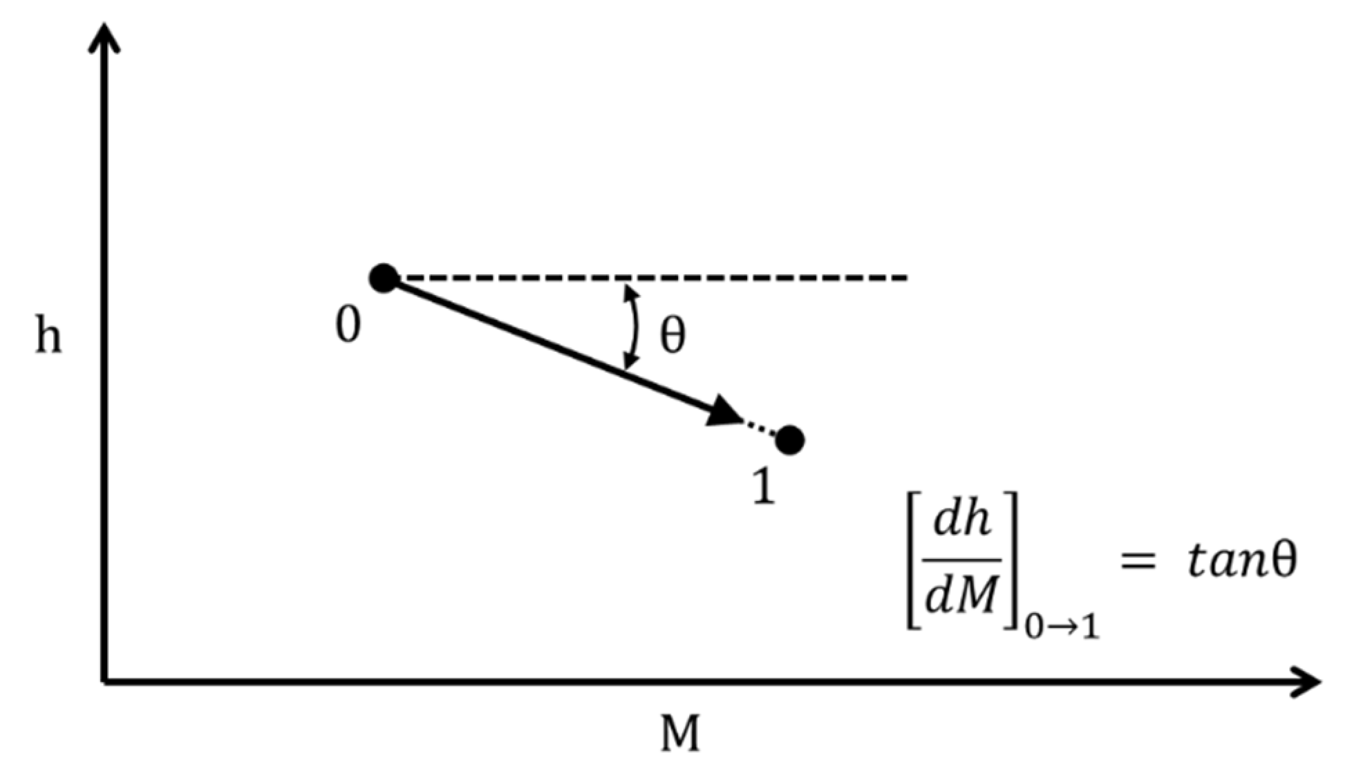
Figure 5.
Schematic representation of the proposed path-tracking method.
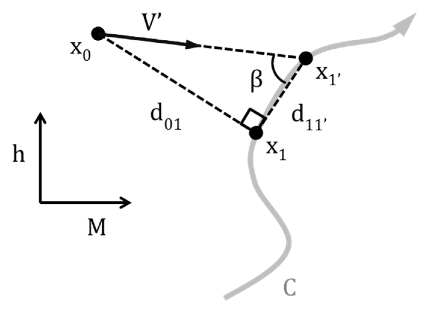
Figure 6.
Path tracking in a supersonic climb example. The climb path is shown in red and the aircraft’s trajectory in black, empty circles corresponding to aircraft position at equal time intervals. The climb path is plotted over contours of Specific Excess Power, expressed in m/s.
Figure 6.
Path tracking in a supersonic climb example. The climb path is shown in red and the aircraft’s trajectory in black, empty circles corresponding to aircraft position at equal time intervals. The climb path is plotted over contours of Specific Excess Power, expressed in m/s.

Figure 7.
System geometry for a circular path.
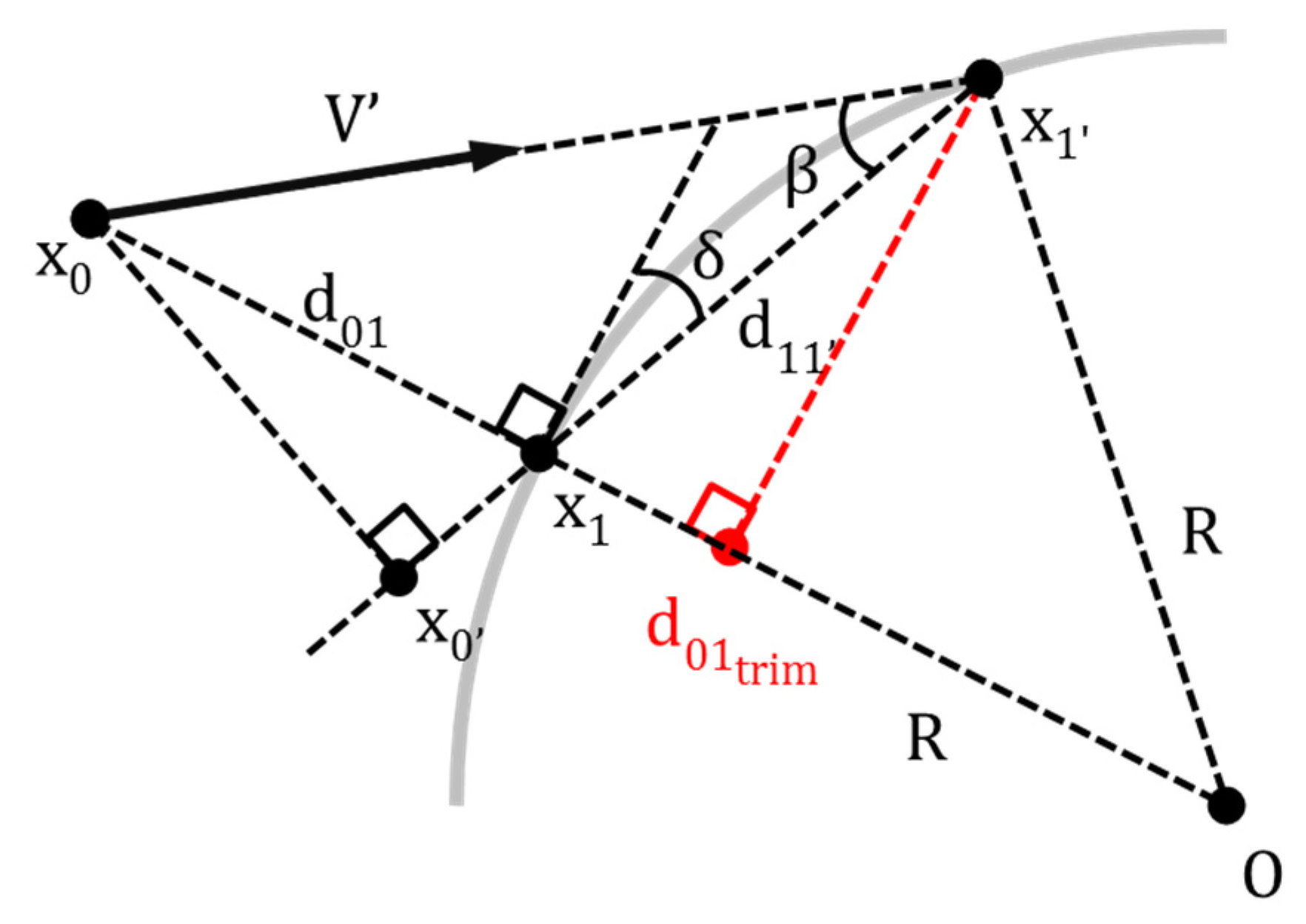
Figure 8.
Altitude (h)–Mach number (M) plots of the climb paths used for simulation validation for: military (a); and maximum (b) power settings. The climb paths are plotted over contours of Specific Excess Power, expressed in m/s.
Figure 8.
Altitude (h)–Mach number (M) plots of the climb paths used for simulation validation for: military (a); and maximum (b) power settings. The climb paths are plotted over contours of Specific Excess Power, expressed in m/s.
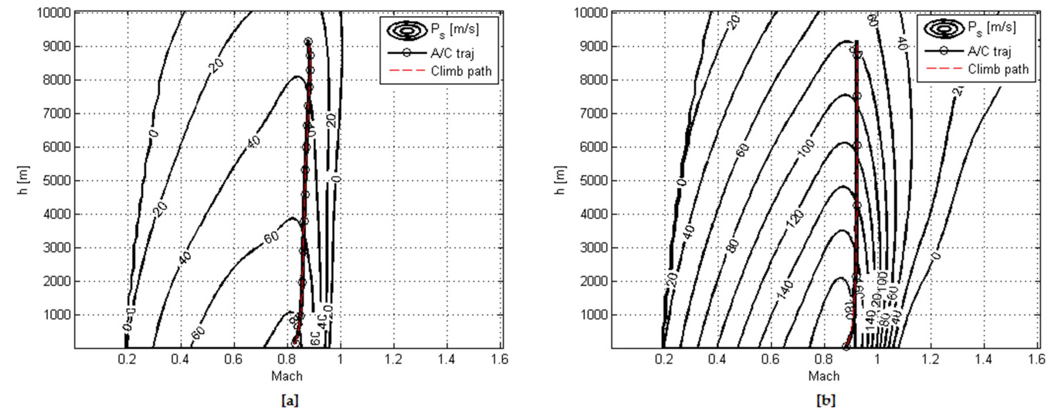
Figure 9.
Flowchart of the proposed two-level optimization scheme.
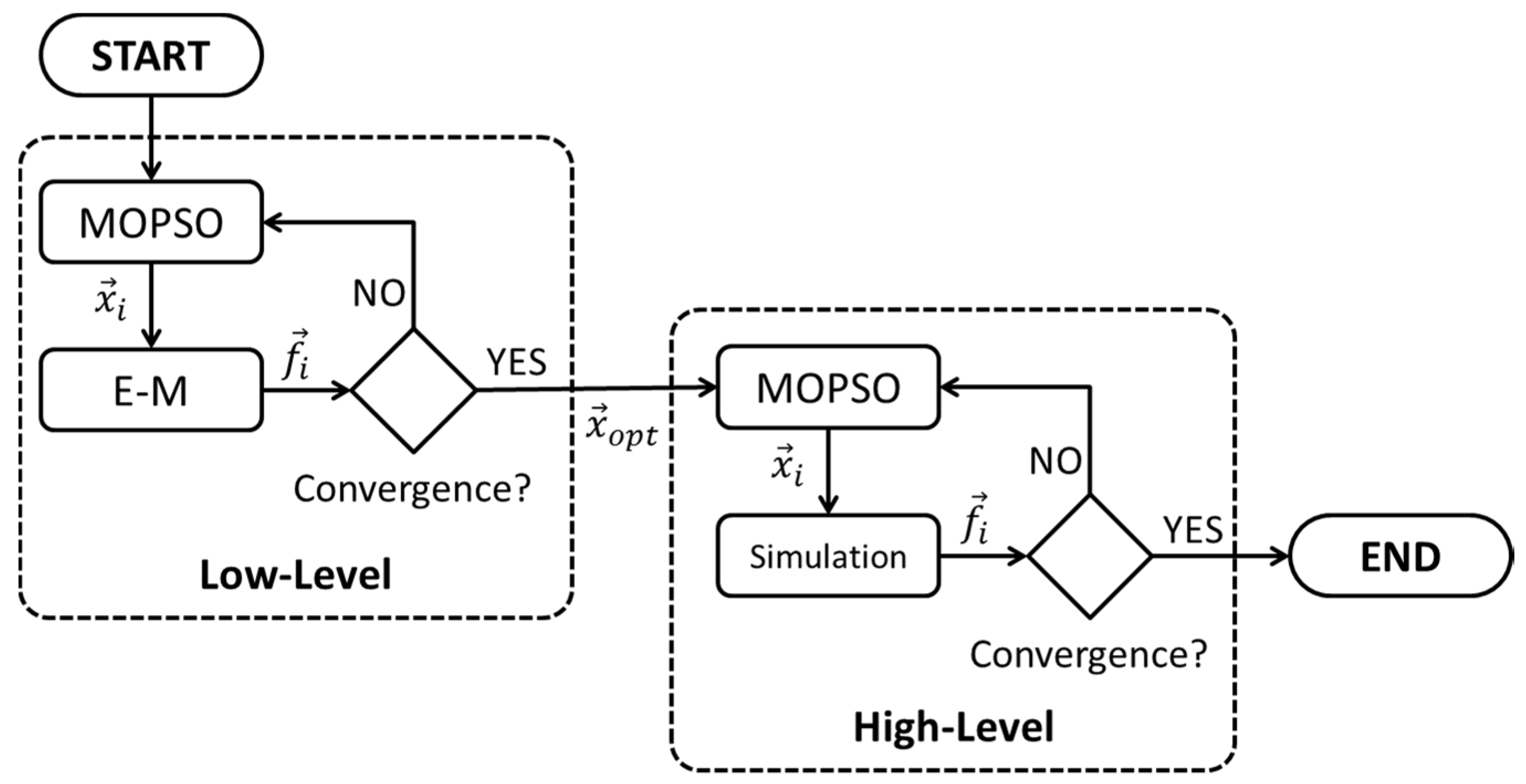
Figure 10.
Convergence of the proposed 2-level MOPSO vs. standard MOPSO in a supersonic climb path optimization problem, using a population of 20 particles; results are averaged from 10 two-objective optimization runs. Iteration counts for the two-level method have been shifted to account for the computational cost of the low-level optimization run. The hypervolume indicator quantifies the part of the objective space (up to a user-defined “nadir” point) dominated by the Pareto front. Higher indicator values correspond to better-placed and/or better-populated fronts.
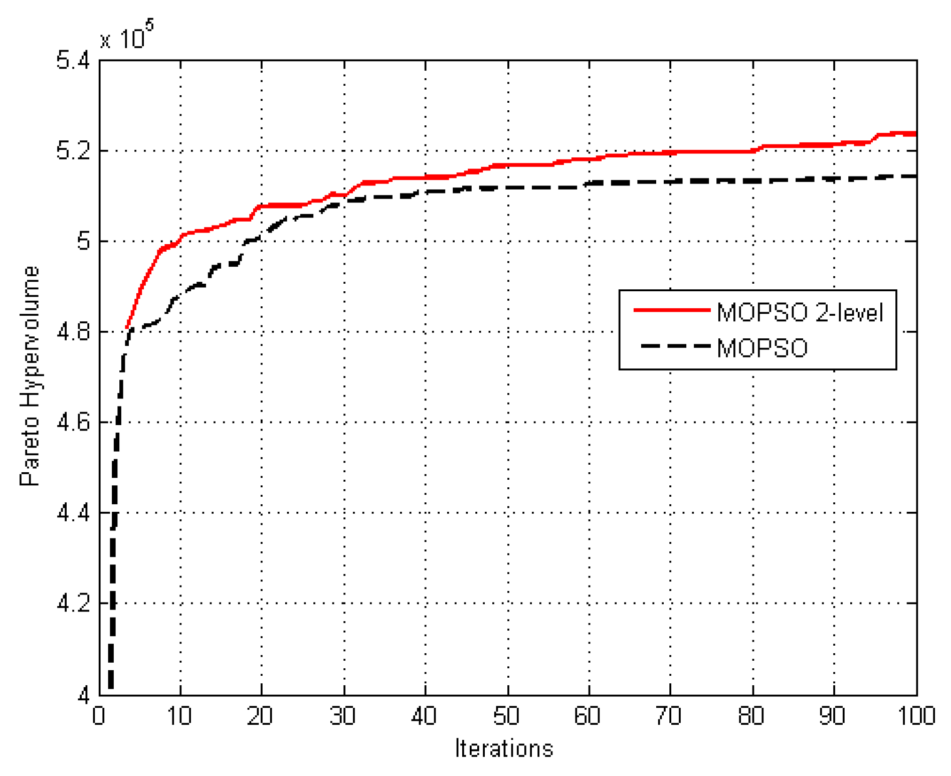
Figure 11.
Pareto front produced by the proposed two-level MOPSO vs. standard MOPSO after 100 iterations, using a 20-particle population.
Figure 11.
Pareto front produced by the proposed two-level MOPSO vs. standard MOPSO after 100 iterations, using a 20-particle population.

Figure 12.
Case A; comparison of fronts of non-dominated solutions obtained for Configurations C1, C2 and C3.
Figure 12.
Case A; comparison of fronts of non-dominated solutions obtained for Configurations C1, C2 and C3.

Figure 13.
Case A, Configuration C1; Minimum Time and Minimum Fuel climb paths, plotted over contours of: Specific Excess Power (m/s) (a); and Energy Efficiency (m/kg) (b).
Figure 13.
Case A, Configuration C1; Minimum Time and Minimum Fuel climb paths, plotted over contours of: Specific Excess Power (m/s) (a); and Energy Efficiency (m/kg) (b).
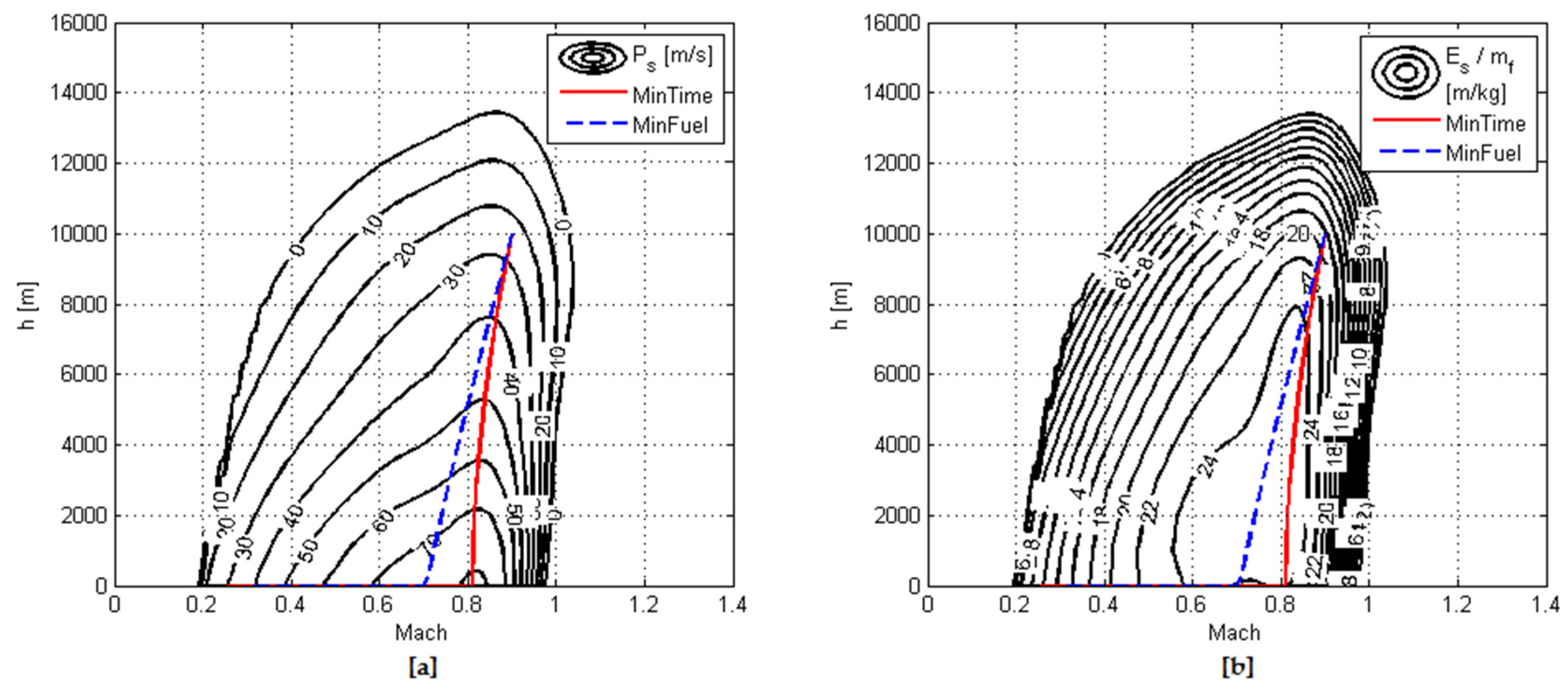
Figure 14.
Case A, Configuration C2; Minimum Time and Minimum Fuel climb paths, plotted over contours of: Specific Excess Power (m/s) (a); and Energy Efficiency (m/kg) (b).
Figure 14.
Case A, Configuration C2; Minimum Time and Minimum Fuel climb paths, plotted over contours of: Specific Excess Power (m/s) (a); and Energy Efficiency (m/kg) (b).
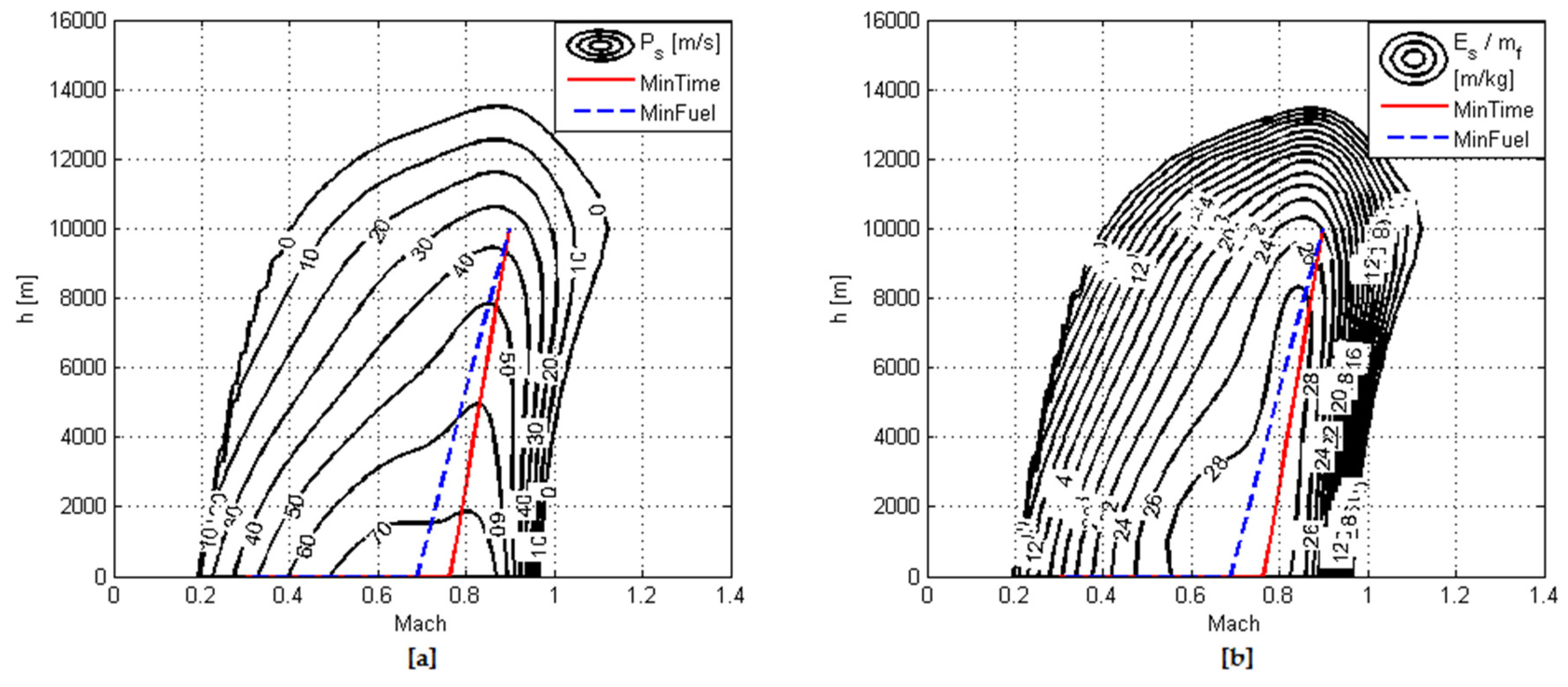
Figure 15.
Case A, Configuration C3; Minimum Time and Minimum Fuel climb paths, plotted over contours of: Specific Excess Power (m/s) (a); and Energy Efficiency (m/kg) (b).
Figure 15.
Case A, Configuration C3; Minimum Time and Minimum Fuel climb paths, plotted over contours of: Specific Excess Power (m/s) (a); and Energy Efficiency (m/kg) (b).
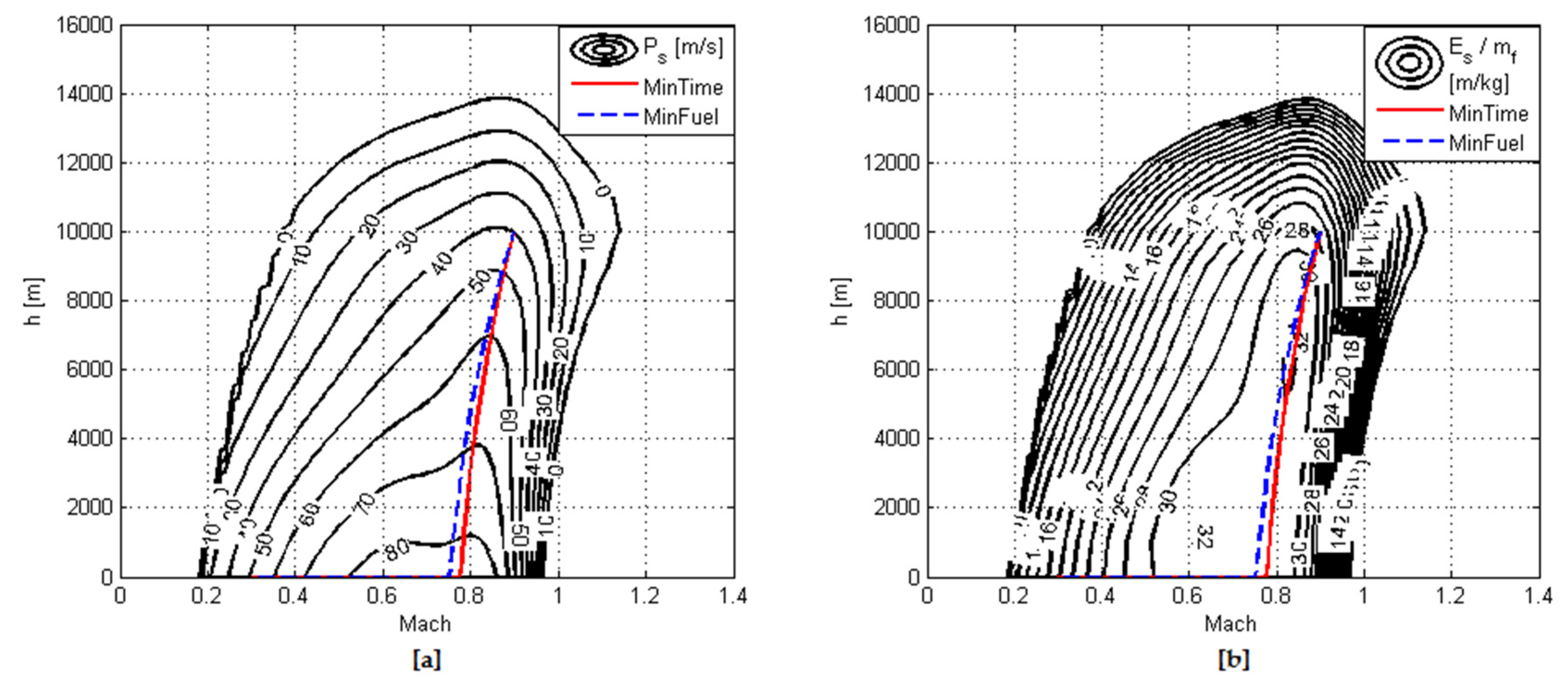
Figure 16.
Case B; comparison of fronts of non-dominated solutions obtained for Configurations C1, C2 and C3.
Figure 16.
Case B; comparison of fronts of non-dominated solutions obtained for Configurations C1, C2 and C3.
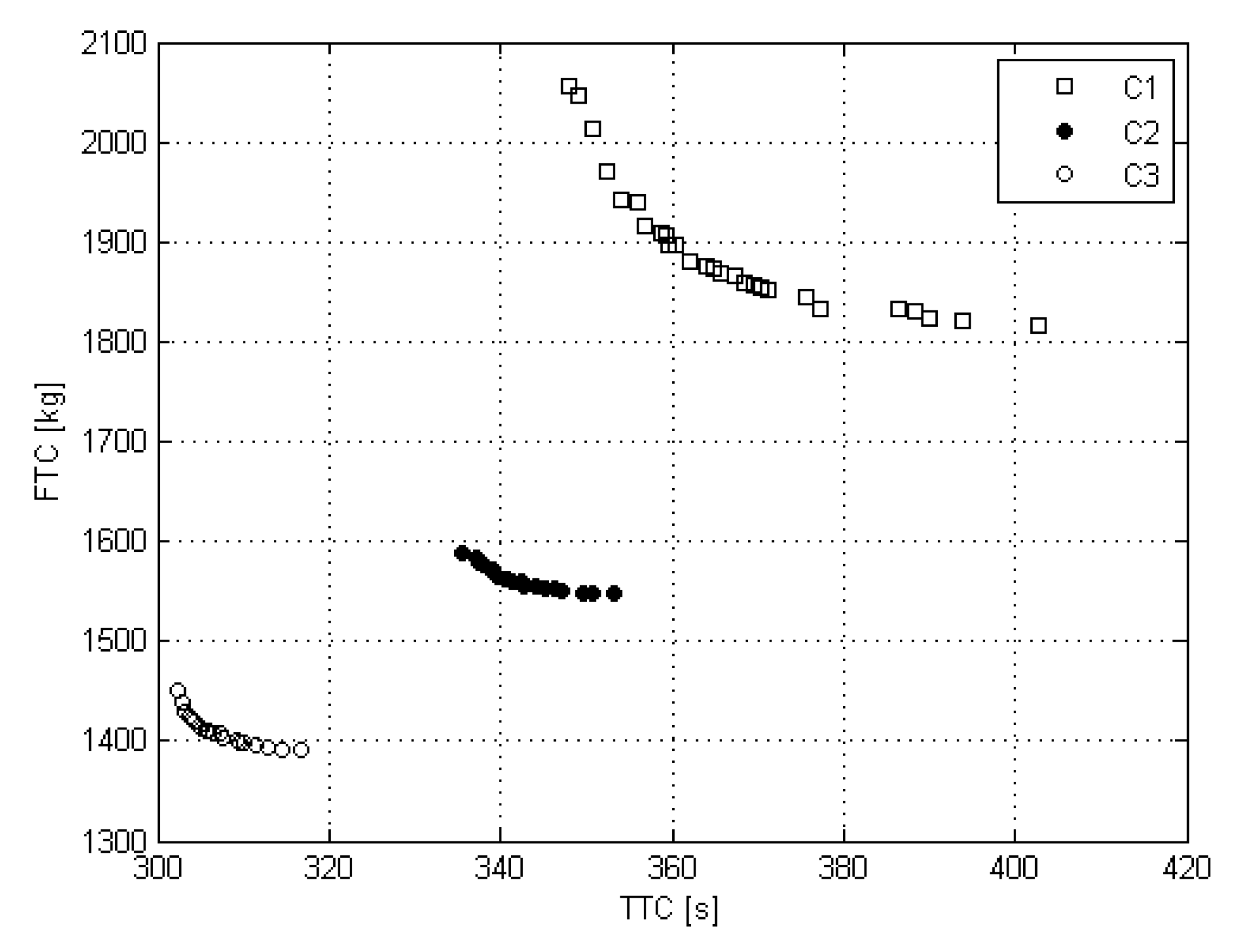
Figure 17.
Case B, Configuration C1; Minimum Time and Minimum Fuel climb paths, plotted over contours of: Specific Excess Power (m/s) (a); and Energy Efficiency (m/kg) (b).
Figure 17.
Case B, Configuration C1; Minimum Time and Minimum Fuel climb paths, plotted over contours of: Specific Excess Power (m/s) (a); and Energy Efficiency (m/kg) (b).

Figure 18.
Case B, Configuration C2; Minimum Time and Minimum Fuel climb paths, plotted over contours of: Specific Excess Power (m/s) (a); and Energy Efficiency (m/kg) (b).
Figure 18.
Case B, Configuration C2; Minimum Time and Minimum Fuel climb paths, plotted over contours of: Specific Excess Power (m/s) (a); and Energy Efficiency (m/kg) (b).
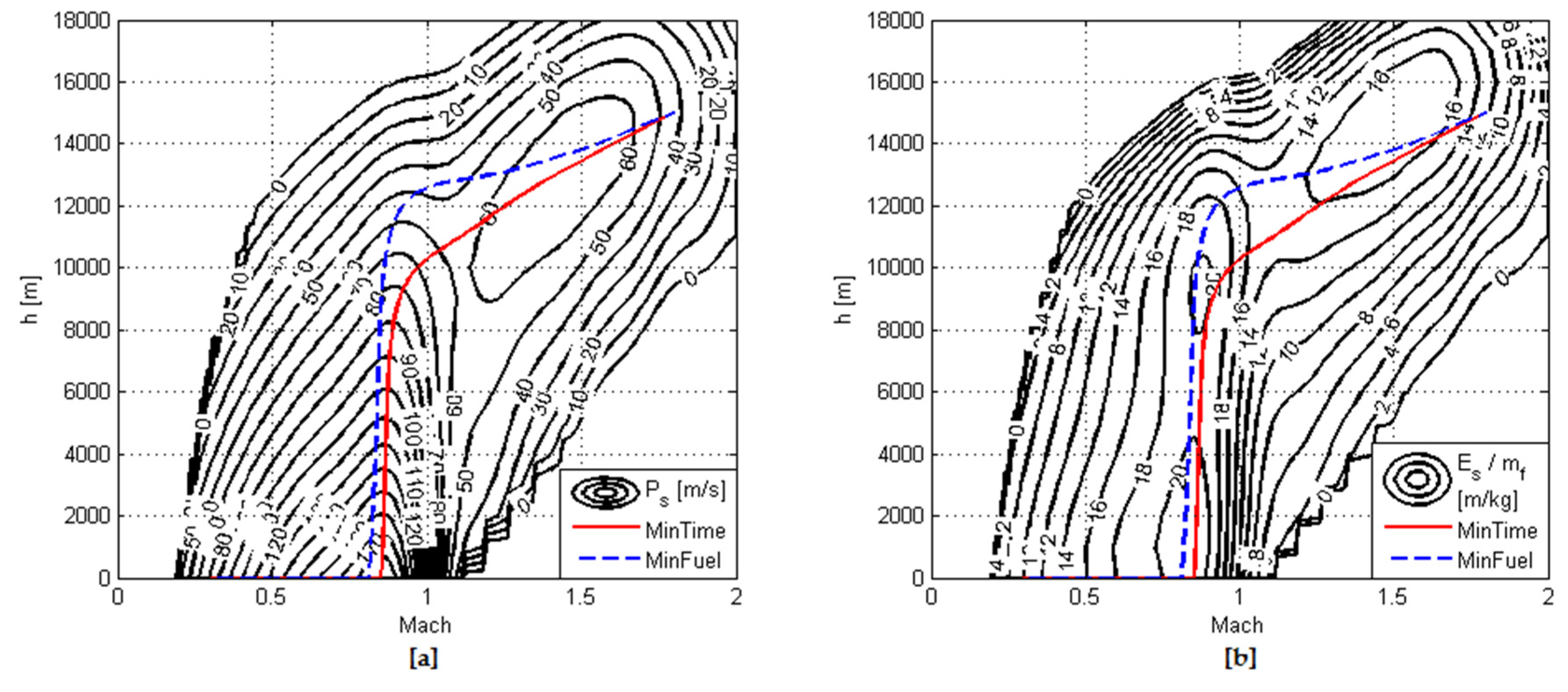
Figure 19.
Case B, Configuration C3; Minimum Time and Minimum Fuel climb paths, plotted over contours of: Specific Excess Power (m/s) (a); and Energy Efficiency (m/kg) (b).
Figure 19.
Case B, Configuration C3; Minimum Time and Minimum Fuel climb paths, plotted over contours of: Specific Excess Power (m/s) (a); and Energy Efficiency (m/kg) (b).

Table 1.
Comparison of simulation results with data from the aircraft’s flight manual for a climb with military power setting for an aircraft AUM of 18,000 kg.
Table 1.
Comparison of simulation results with data from the aircraft’s flight manual for a climb with military power setting for an aircraft AUM of 18,000 kg.
| Altitude [ft] | Time To Climb [min] | Fuel To Climb [kg] | ||||
|---|---|---|---|---|---|---|
| Sim | Manual | %Error | Sim | Manual | %Error | |
Table 2.
Comparison of simulation results with data from the aircraft’s flight manual for a climb with maximum power setting for an aircraft AUM of 18,000 kg.
Table 2.
Comparison of simulation results with data from the aircraft’s flight manual for a climb with maximum power setting for an aircraft AUM of 18,000 kg.
| Altitude [ft] | Time To Climb [min] | Fuel To Climb [kg] | ||||
|---|---|---|---|---|---|---|
| Sim | Manual | %Error | Sim | Manual | %Error | |
Table 3.
Convergence of the proposed 2-level MOPSO vs. standard MOPSO after 100 iterations; Statistics have been derived from 10 optimization runs for each method.
Table 3.
Convergence of the proposed 2-level MOPSO vs. standard MOPSO after 100 iterations; Statistics have been derived from 10 optimization runs for each method.
| Method | Hypervolume Indicator | |
|---|---|---|
| Mean | Std. Dev. | |
| - | ||
Table 4.
Specifications of the examined configurations.
| Configuration | Engine Type | Mass [kg] | ||
|---|---|---|---|---|
| Airframe + Fuel | Engines | Total | ||
Table 5.
Test case specifications.
| Case | Thrust Setting | Start | End | ||
|---|---|---|---|---|---|
| Mach | Alt [m] | Mach | Alt [m] | ||
© 2017 by the authors. Licensee MDPI, Basel, Switzerland. This article is an open access article distributed under the terms and conditions of the Creative Commons Attribution (CC BY) license (http://creativecommons.org/licenses/by/4.0/).
Share and Cite
MDPI and ACS Style
Antonakis, A.; Nikolaidis, T.; Pilidis, P. Multi-Objective Climb Path Optimization for Aircraft/Engine Integration Using Particle Swarm Optimization. Appl. Sci. 2017, 7, 469. https://doi.org/10.3390/app7050469
AMA Style
Antonakis A, Nikolaidis T, Pilidis P. Multi-Objective Climb Path Optimization for Aircraft/Engine Integration Using Particle Swarm Optimization. Applied Sciences. 2017; 7(5):469. https://doi.org/10.3390/app7050469
Chicago/Turabian StyleAntonakis, Aristeidis, Theoklis Nikolaidis, and Pericles Pilidis. 2017. "Multi-Objective Climb Path Optimization for Aircraft/Engine Integration Using Particle Swarm Optimization" Applied Sciences 7, no. 5: 469. https://doi.org/10.3390/app7050469
Note that from the first issue of 2016, this journal uses article numbers instead of page numbers. See further details here.