
Separation Control on a Bridge Box Girder Using a Bypass Passive Jet Flow


1
School of Civil Engineering, Northeast Forestry University, Harbin 150040, China
2
Key Lab of Smart Prevention and Mitigation of Civil Engineering Disasters of the Ministry of Industry and Information Technology, Harbin Institute of Technology, Harbin 150090, China
3
Key Lab of Structures Dynamic Behavior and Control of Ministry of Education, Harbin Institute of Technology, Harbin 150090, China
*
Author to whom correspondence should be addressed.
Appl. Sci. 2017, 7(6), 501; https://doi.org/10.3390/app7060501
Submission received: 2 March 2017
/
Revised: 6 May 2017
/
Accepted: 9 May 2017
/
Published: 24 May 2017
Abstract
:In the present study, a bypass passive jet flow control method was proposed to mitigate unsteady wind loads and to manipulate the flow field around a single box girder of a bridge. With a geometric ratio of 1:125, the single box girder model was determined using the cross-section of the Great Belt East Bridge. During the experiments, one test model without control was adopted, while five different test models with different suction/jet configurations were employed to analyze the effects of the control method and to reveal the underlying mechanism of different control schemes. The incoming wind speed was fixed to 12 m/s and the wind attack angles were changed from −20° to 20°, resulting in a corresponding Reynolds number of Re = 0.28 × 10⁵–0.74 × 10⁵ based on the different attack angles. A six-component force balance, a set of digital sensor array (DSA) pressure transducers, and a particle image velocimetry (PIV) system was used to measure the aerodynamic forces, pressure distributions, and flow fields around the test models to evaluate the control effectiveness of different control cases. Detailed flow structures are presented and discussed for two test cases when the angles of attack are +15° and −20°. The effects of control on the aerodynamic forces were first investigated to determine and select the best one out of five control cases. The pressure distributions on the surface of the test model without control and the best control case were then compared to evaluate the control effectiveness of the pressure gradient and the fluctuating pressure coefficients. The flow fields around the test models demonstrate that the bypass passive jet flow control could decrease vortex strength, delay flow separation, and change recirculation region and size. The results of the aerodynamic forces, pressure distributions, and flow fields indicate that the bypass passive jet flow control method results in effective control.
1. Introduction
Long-span bridges are usually adopted to allow people to cross rivers or straits, and have been widely built throughout the whole world. In particular, a considerable amount of large-span bridges (i.e., suspension bridges and cable-stayed bridges) have been constructed or are under construction in China, with the rapid development of the economy in the last three decades. However, with an increase in span, long-span bridges become more flexible and more prone to vibrating under unsteady wind loads. Although the cross-section of a single box girder is generally designed to be similar to a streamline, the alternating vortex shedding from the upper and lower surfaces of the girder cannot be completely eliminated and will probably result in vortex-induced vibrations (VIVs) [1].
There can be different behaviors of frequent VIVs in long-span bridges because of differences in the cross-sections of the main girders [2,3,4]. However, unsteady vortex shedding from the girders should be mainly responsible for the occurrence of VIVs. Larsen et al. [5] performed a field investigation on the VIV of the Great Belt East Bridge (Storebælt Suspension Bridge) in Denmark. This bridge was often observed to vibrate in low wind speeds of 4–12 m/s, with the single mode vibrations of a relatively large amplitude excited by vortex shedding. Fujino and Yoshitaka [6] observed a significant vibration due to vortex shedding on the Trans-Tokyo Bay Crossing Bridge. The first-mode VIV with a maximum amplitude exceeding 50 cm peaked at the wind speed of 16–17 m/s. Li et al. [7] conducted a field measurement on the Xihoumen Suspension Bridge, which is the longest suspension bridge in China. The investigation results indicated that the VIV occurred more frequently at a low wind speed range of 6–10 m/s, with the wind direction being nearly perpendicular to the bridge axial line. As mentioned in the above three bridges, the VIVs of these long-span bridges occurred at wind speeds of 4–17 m/s, which was a frequent in-situ wind speed range at these bridges. It could be concluded that the VIVs will frequently appear at low speeds if there are no control measures implemented on these bridges.
Two kinds of control strategies (i.e., active and passive control methods) have been developed to mitigate the wind-induced vibrations of long-span bridges. Larsen et al. [8] designed tuned mass dampers (TMDs) to control the potential wind-induced vibrations of the Great Belt East Bridge. The time-domain simulation results indicated that the girder and TMD responses did not exceed the maximum allowable values. The TMDs were then applied to control the VIVs of the Rio-Niterói Bridge in Rio de Janeiro, Brazil [9,10]. The numerical simulation results showed that the TMDs under active control had a better performance in reducing and controlling the responses of the VIVs. Zhang et al. [11] employed an active span-wise suction method to control the vortex shedding from the test models of the Great Belt East Bridge.
The alternative approach was the passive aerodynamic method, which employed accessory components on the bridges, such as guide vanes [5] and wing plates [12,13] to improve aerodynamic performance. It was found that the guide vanes were effective in suppressing vortex-induced vertical oscillations of the suspension bridge of the Great Belt Bridge, as reported in Larsen et al. [5]. In addition, the airflow around the main girder could be modified by attaching or adjusting some non-structural parts (such as railings, parapets, maintenance rails and collision barriers) with specific shapes at the specific positions of the main girder [14,15]. El-Gammal et al. [16] used the span-wise sinusoidal perturbation method (SPPM) module in both the leading and trailing edges of the plate girder bridge. The experimental results indicated that VIV responses could be dramatically suppressed with higher wave steepness.
Based on the research findings by Baek and Karniadakis [17] and Chen et al. [18], a bypass passive jet flow control method was proposed to control the flow field around the test models of the Great Belt East Bridge in the present study. Different from the study of Baek and Karniadakis [17] and Chen et al. [18], the challenge of the present flow control is that the connected channel set in the bridge deck has a relatively longer length with a larger fluid resistance than that of the circular cylinder; moreover, the present flow control need be beneficial in manipulating the separated flow of the bridge deck at different angles of attack. Therefore, it is necessary to investigate the underlying mechanism of bypass passive jet flow control for a bridge deck. The control principles of this method are described as follows. First, the suction/jet holes were set at a region close to the leading/trailing edges of the test models, respectively, with the suction holes connected to the jet holes through the bypass channels. The incoming airflow entered from the suction holes, progressed through the channels, and then blew out from the jet hole into the wake flow. Thus, the flow would be modified and the aerodynamic effects changed.
2. Experiment Setup and Model Configuration
2.1. Model Configuration
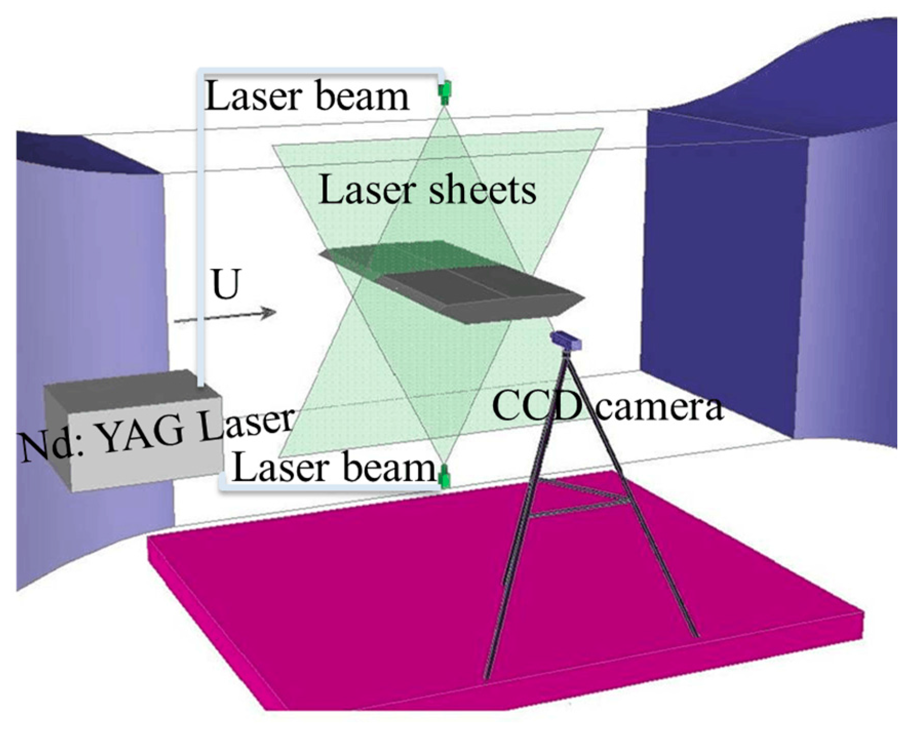
The experiment was conducted in a small-scale closed-circuit wind tunnel, i.e., SMC-WT1 (Harbin Institute of Technology, Harbin, China) at the Joint Laboratory of Wind Tunnel and Wave Flume, Harbin Institute of Technology. The test section was made of transparent plexiglass with a cross-section of 505 mm × 505 mm and length of 1050 mm, as shown in Figure 1. The wind speed can be continuously adjusted from 0 to 25 m/s with minimum steps of 0.05 m/s, and the turbulence intensity of the incoming airflow is less than 0.4%.
The Great Belt East Bridge in Denmark is the third longest suspension bridge in the world with a main span of 1624 m. The cross-section of the main girder is a single box with a width and height of 31.0 m and 4.34 m, respectively. With a relatively small aspect ratio (width/height), VIVs excited by the vortex shedding excitation at a low wind speed range of 4–12 m/s was observed in this bridge [5]. Therefore, the main girder of the Great Belt East Bridge was chosen for the research objective in the present experimental study. A high-precision 3D printing technology was employed to manufacture a segment model of the main girder by using a PLA (polylactic acid) plastic material. A geometric scale ratio of 1:125 was determined, although it was relatively smaller because of the limitation of the test section size. Scaling the model by a factor of 125 has an impact on the Reynolds number of the flow. As reviewed by Larose and D’Auteuil [19], the Reynolds number sensitivity of the aerodynamics of bluff bodies with sharp edges and concluded that ignoring the Reynolds number effect of bluff bodies such as box-like bridge decks can lead to systematic errors. Larsen et al. [20] conducted an investigation on the vortex characteristics of a twin box bridge section at different Reynolds numbers. In our group, the Reynolds number effects of twin-box girders have always been a hot topic. A recent report can be found in Li et al. [21].It should be mentioned that we could never reach the real Reynolds number level in the atmospheric boundary layer wind tunnel, due to the limitations of test section and the maximum wind speed. We also noticed that the Reynolds number was much smaller in comparison with real bridges. However, the present study focuses on the fundamental side, and we aim to reveal the flow characteristics around the scaled models with and without control. For the segment model, the accessory members of the single box girder bridge were neglected and the slope of the upper surface was considered as shown in Figure 2.
Figure 2a shows the geometric information for the cross-section of the segment model, where the width and height are 248.0 mm and 34.7 mm, respectively, according to the geometric scale ratio. The dimension of the segment model in the span-wise direction is 480.0 mm, due to the size limitation of the test section. With this relatively small aspect ratio, the vortex shedding of the test segment model will be easily observed, and the potential vortex-induced vibration can be controlled when the alternating vortex shedding is suppressed. In the present study, a bypass passive jet flow control method was proposed to manipulate the vortex shedding in the test model.
Five test models with bypass passive jet flow control are shown in Figure 2b–f, respectively. The test models for the five control cases have the same external dimensions as Case 0 (Figure 2a). To transport the airflow from the positive side to the negative pressure region and ensure that the upper surface of the girder is not affected, suction/jet holes were only manufactured on the leading/trailing edges of the test models, respectively, which were connected by the hollow channels. As shown in Figure 2e, the height of the connected channel is 2.5 mm, the thickness of the wall is 1.5 mm, and the height of the suction/jet hole is one tenth of the cross-sectional height of the test model (i.e., 3.47 mm). The three suction/jet holes are equidistantly-distributed on the leading and trailing edges of the lower surface. The suction/jet holes of the upper surface are set on the center of the leading/trailing edges of the lower surface, respectively. Combined with Figure 2b–f, the five proposed control schemes are listed in Table 1.
In order to evaluate the effectiveness of the control for the five different control schemes, a non-dimensional suction/jet momentum coefficient Jsuc was defined in the present study as follows:
where N = 1–3 is the suction/jet hole number on the leading or trailing edge of the lower surface in the cross-section; n = 16 is the suction/jet hole number along the span-wise direction; HUsuc is the height of the suction/jet hole on the upper surface; HLsuc is the height of the suction/jet hole on the lower surface; Lsuc is the length of the suction/jet hole; H is the height of the cross-section of the test model; and L is the span-wise length along the test model.
The suction/jet momentum coefficients for the five control cases and Case 0 are listed in Table 1.
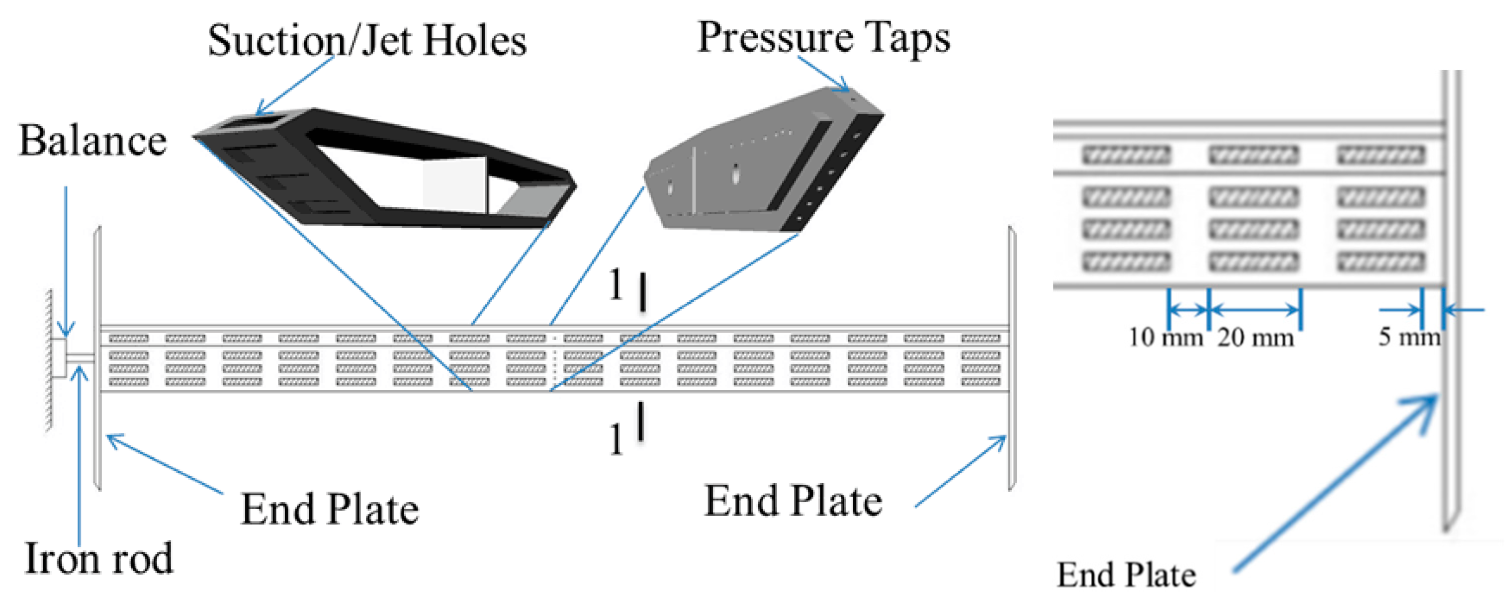
Figure 3 provides a view of the model from the downstream side. Two end plates were installed on both ends of the model to avoid the effects of having free ends and to improve the accuracy of the test results. The length of the suction/jet holes is 20 mm in the span-wise direction, the distance between two neighboring suction/jet holes is 10 mm along the span-wise direction, while the suction/jet holes at both ends are 5 mm from the edge of the model.
2.2. Experimental Setup for Aerodynamic Force Measurements
A six-component force balance (Model Gamma SI-600-60, ATI Industrial Automation) was employed to obtain the values for all aerodynamic forces (i.e., lift, drag and moment of the test models, Figure 3). The force balance was mounted on a frame outside the wind tunnel using a threaded iron rod. The sampling frequency and time of the force balance were set to 1000 Hz and 90 s, respectively.
The lift, drag, and moment coefficients (i.e.,, and can be obtained by applying aerodynamic forces to the test models at different wind attack angles, as follows:
where = 12 m/s is the wind speed of the incoming airflow, which is calculated by the static pressure and total pressure tested by a Pitot tube; B is the width of the test model; is the air density, which was chosen as ; and , and are the drag, lift, and moment per unit length, respectively.
2.3. Experimental Setup for Pressure Measurements
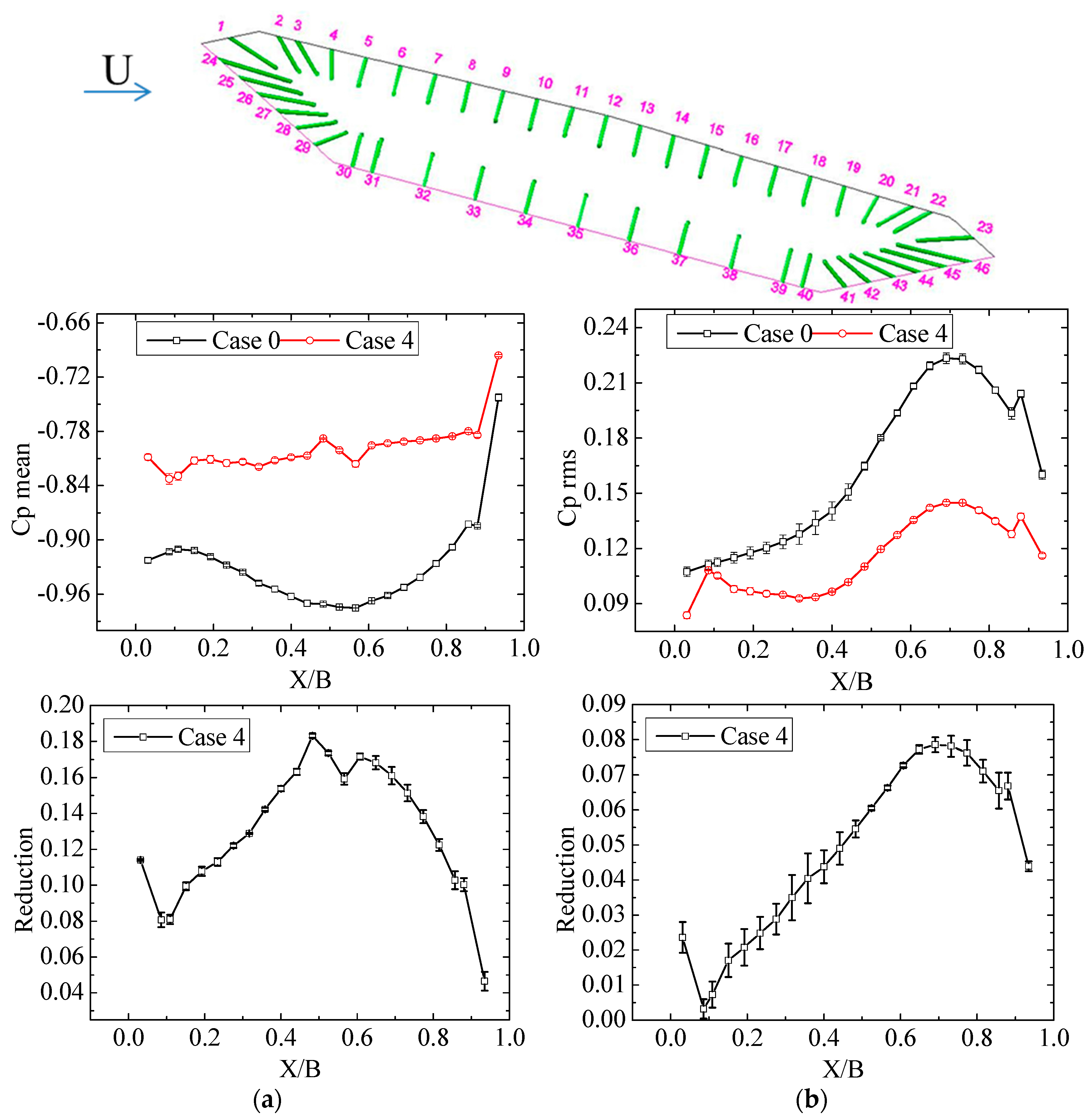
The pressure measurement section was located at the center of the test model (Figure 3). In the present study, 46 taps were arranged around the pressure measurement section (Figure 4). The pressure taps were connected to three units of digital sensor arrays (DSA3217, Scanivalve Corp®, Liberty Lake, WA, USA) by using polyvinyl chloride (PVC) tubes for pressure data acquisition. These PVC tubes had an internal diameter of 0.9 mm and a length of 0.5 m. The precision of the DSA 3217 Model is ±0.05% of the full-scale range (±10 inches of H2O). During the surface pressure measurements, the sampling frequency and time of each pressure tap were set as 312.5 Hz and 32 s, respectively. Based on the work of Irwin et al. [22] and Chen et al. [18], it can be expected that there are relatively small and negligible effects of the tubing system on the pressure measurements for the present test cases, such as the amplitude, attenuation and the phase lag of the instantaneous pressure signals. However, the blockage ratios were 6.67–17.85%, which correspond to the wind attack angle range of 0–20° in the current study. The solid blockage and the wake blockage effects of the test models on the pressure measurements were corrected, as suggested by Barlow et al. [23].
The pressure coefficients distributed around the surface of the test models can be obtained by the pressure measurement system as follows:
where is the surface static pressure on the test model and is the static pressure at the inlet of the test section.
2.4. Experimental Setup for PIV Measurements
In addition to the aerodynamic forces with a six-component force balance and the surface pressure measurements with the DSA pressure transducers, a particle imaging velocimetry (PIV) technique was employed to characterize the flow characteristics of the test models with and without control. The laser plane was located at the center of the seventh row of suction/jet holes, which were numbered from right to left in the span-wise direction (Figure 3). The experimental setup of PIV measurements is illustrated in Figure 1.
During the PIV measurements, the incoming airflow was seeded with 1–5 µm oil droplets by using a droplet generator. It was checked whether the seeding particles mixed thoroughly and uniformly or not (i.e., homogeneous seeding) during the experiments. The seeding density was found to be adequate for interrogation with interrogation regions of 32 × 32 pixels. This kind of particle seeding has been a long established method. Identical fog machines, oils, and set-ups have been used in a number of previous studies (e.g., [18,24,25,26,27]). In addition, as proposed in Samimy and Lele [28], that particle response could be well characterized by , the ratio of particle response time to the flow time scale (Stokes’ number), and only particles with > 0.05 were found to misrepresent the flow features. In the present experiment, is estimated as: , which is less than 0.05. Therefore, we believe the particle movement is able to represent the fluid velocity.
Illumination was provided by a double-pulsed Nd:YAG laser (Vlite 200, Beamtech Optronics Co., Ltd., Beijing, China), which emitted two pulses of 200 mJ at the wavelength of 532 nm with a repetition rate of 2 Hz. The laser sheet was generated by a set of mirrors as well as spherical and cylindrical lenses, which can shape the emitting laser beam. In the measured region, the thickness of the laser sheet was about 1.0 mm. Using two independent laser arms, two laser sheets generated by one laser were manipulated to illuminate both the upper and lower sides of the test models. The laser energy was divided into two parts. This system was elaborately designed and carefully examined by the laser manufacturer. When the center of the target plane was about 1050 mm away from the lens of the laser arms, the laser energy reached the maximum. A 14-bit (1600 × 1200 pixels) CCD (charge-coupled device) camera (pco.1600, PCO AG., Kelheim, Germany) was used to record images for the PIV measurements. The CCD camera and double-pulsed Nd:YAG lasers were connected to a workstation (host computer) via a Digital Delay Generator (Model 575-8C, Berkeley Nucleonics, San Rafael, CA, USA), which controlled the timing of the laser illumination and the image acquisition. The CCD camera was carefully aligned and was perpendicular to the laser planes using the spirit level.
Instantaneous velocity vectors can be obtained by frame-to-frame cross-correlation operation of the images obtained by the PIV system. The MATLAB codes to process the PIV images were developed by the third author and Hui Hu of Iowa State University [18,24,26,29]. There was another post-processing step for filtering/deletion of spurious vectors after image processing. However, the experimental results were maintained high-quality, as the valid vectors are mostly calculated to be about 98% in the present experiment.
In the cross-correlation operation, a 32 × 32 pixel interrogation window was adopted, with the interrogation window overlapped by 50%. When the instantaneous velocity vector (u, v) in the flow field was determined, the corresponding span-wise vorticity could be calculated. In each case, the mean velocity, turbulent kinetic energy (), swirling strength, separation point, and other flow field characteristics were then obtained from instantaneous PIV measurements. Three-hundred pairs of images were collected for each case during the experiments. The image had a physical area of 338 mm × 254 mm. The interrogation window was 32 × 32 pixels, corresponding to an area of 7 mm × 7 mm. Since an effective overlap of 50% of the interrogation windows was adopted in PIV image processing, the resultant spatial resolution was 3.5 mm × 3.5 mm for the PIV measurements. In this experiment, the uncertainty of instantaneous velocity measurements was about 5.43%.
3. Results and Discussion
3.1. Analysis of Aerodynamic Coefficients
After acquiring the aerodynamic forces by a six-component force balance, the mean values (i.e., Cl_mean, Cd_mean, and Cm_mean) and the fluctuations (i.e., Cl_rms, Cd_rms, and Cm_rms) of the instantaneous aerodynamic force coefficients were obtained through statistical analysis. In the present study, Cd_mean was measured to be 0.061 at a wind attack angle of 0°, which is close to the result of 0.064 from Taylor et al. [4] and the numerical simulation result of 0.060 from Frandsen [30].
Figure 5 shows the mean values of the lift, drag, and moment coefficients for all test models at wind attack angles ranging from −20° to 20°. The reduction of aerodynamic coefficients is defined as:
When reduction is close to zero, it means this modification has little effect on the Case 0 model. For the mean drag coefficient, the five control cases are close to the Case 0, although there is a small difference at a large negative attack angle (e.g., −20°). With respect to the mean lift coefficient, control cases 2–5 achieved a small reduction while the Case 1 had no distinct change compared with the Case 0 at negative attack angles. For this mean lift coefficient, the control cases 2–4 also had a reduction, while control cases 1 and 5 were close to Case 0 at positive attack angles. For the mean moment coefficient at negative attack angles, control cases 2–5 achieved a decrease and Case 1 had no noticeable change in comparison with Case 0. At positive attack angles, Case 5 was close to Case 0, while the other control cases achieved a distinct decrease.
Figure 6 illustrates the fluctuations (RMSs: root-mean-square values) of the lift, drag, and moment coefficients for all test models at the wind attack angle range of [−20°, 20°]. At a large negative attack angle (e.g., −20°), the control effectiveness of the five control cases is [17.91%, 70.16%, 71.41%, 83.73%, 18.81%]; [16.32%, 66.73%, 68.65%, 93.15%, 6.59%]; and [4.13%, 59.45%, 61.52%, 65.28%, 25.22%] for the lift, drag, and moment coefficient RMSs, respectively. Control cases 2–4 had a large decrease in the RMSs of the aerodynamic coefficients, while Case 4 had the best control effectiveness. Cases 1 and 5 had a small control effectiveness, because the suction/jet holes were only located on the upper or lower surfaces.
For Case 0 at positive attack angles, the peaks appear at the angle of 15° for the lift and drag coefficients, with the maximum value occurring at the angle of 10°. For the peak value suppression at the angle of 15°, the control effectiveness of the five control cases is [7.04%, 19.29%, 12.38%, 23.25%, 8.53%]; [9.32%, 15.65%, 9.09%, 18.76%, 5.91%]; and [15.00%, 24.98%, 25.57%, 25.55%, 7.37%] for the lift, drag, and moment coefficient RMSs, respectively. Control cases 3 and 4 are better than the other control cases. Combining the control effectiveness at the angles of −20° and 15°, Case 4 should be the best control case.
Following this, the integral of the Cm_mean along a wind attack angle from −20° to 20° was performed to evaluate the work done by the moment (Table 2). The results indicate that control cases 2–4 had smaller values compared to Case 0, while Case 4 had the smallest value, which indicates the best control effectiveness.
According to the above analysis, further pressure distributions and flow structures around the test models will focus on the best control case (Case 4) at two larger wind angles of −20° and 15°. The control philosophy in the present study was to form a communicating channel between the windward and leeward surface of the test model and to generate a passive jet into the wake. The transportation capability of flow between windward decides the flow control effectiveness. With more holes being manufactured, the fluid transporting capacity was more powerful and the interaction between the jet vortex and wake flow was enhanced. Similar findings have been discussed in Chen et al. [18] and Gao et al. [31].
3.2. Analysis of Surface Pressure Distributions
Figure 7 shows comparisons of the distributions of the mean and fluctuating pressure coefficients around the test models with and without control at a negative wind attack angle of −20°. As shown in Figure 7a, the mean pressure coefficients on the upper surface of Case 0 and Case 4 are close to each other. Furthermore, the pressure gradients are positive and the flow will not separate from the upper surface. For Case 0, the fluctuating pressure coefficients are smaller on the windward side on the upper surface, as shown in Figure 7b. In the region near the trailing edge of the upper surface, the fluctuating pressure coefficients were relatively larger, which may be induced by the interaction between the alternating wake flows from the upper and lower surfaces. The fluctuating pressure coefficients on the upper surface of the test model in control Case 4 were slightly lower compared to Case 0.
At the negative attack angle of −20°, the flow separation is mainly located on the lower surface. On the windward side of the lower surface, the adverse pressure gradient region of the Case 4 is wider than the Case 0 (Figure 7c), resulting in decreased fluctuating pressure coefficients in this region compared to the Case 0 results (Figure 7d). However, on the leeward side of the lower surface, the pressure gradients of Case 4 are decreased and the fluctuating pressure coefficients obtain a great reduction in comparison with Case 0 (Figure 7c,d). Combining the fluctuating pressure coefficients on the whole lower surface, the total aerodynamic force coefficients (i.e., the lift, drag, and moment coefficients) should be greatly reduced in the Case 4, which has also been validated by the results in Figure 6.
Figure 8 presents the comparisons of the distributions of the mean and fluctuating pressure coefficients around the test models with and without control at a positive wind attack angle of 15°. At this angle, the flow separation is mainly located on the upper surface. On the leeward side of the upper surface, there is a large decrease in mean pressure coefficients and the adverse pressure gradient obtains an obvious reduction (Figure 8a). Following this, there is a dramatic decrease in fluctuating pressure coefficients of Case 4 compared to Case 0 results, as shown in Figure 8d.
The results shown in Figure 8c,d are similar to those in Figure 7a,b. The mean pressure coefficient distributions of Case 0 and Case 4 are close to each other. The fluctuating pressure coefficients are slightly smaller than the results of Case 0, as shown in Figure 8c,d.
Combining the results in Figure 7 and Figure 8, it was found that the control Case 4 has less influence on the surface without a flow separation and greater effects on the surface with a flow separation. The control Case 4 can greatly decrease the adverse pressure gradient and fluctuating pressure coefficients. The reason mainly includes two aspects: first, the main flow on the surface without a flow separation will have the same movement direction as the jet flow. Therefore, the jet flow will hardly prevent or influence the main flow. Secondly, it is important to consider the main flow on the surface with a flow separation. In particular, the main flow has a reverse direction with the jet flow in the separation region. Thus, the interaction between the jet flow with the main flow will greatly influence the pressure distributions.
3.3. Analysis of PIV Experimental Results
As described above, a PIV system was used to measure the flow field to further understand the underlying mechanism of the bypass passive jet flow control. Similar to the analysis of the pressure distribution, the PIV experimental results also focus on Case 4 and Case 0 under two wind attack angles of −20° and 15°.
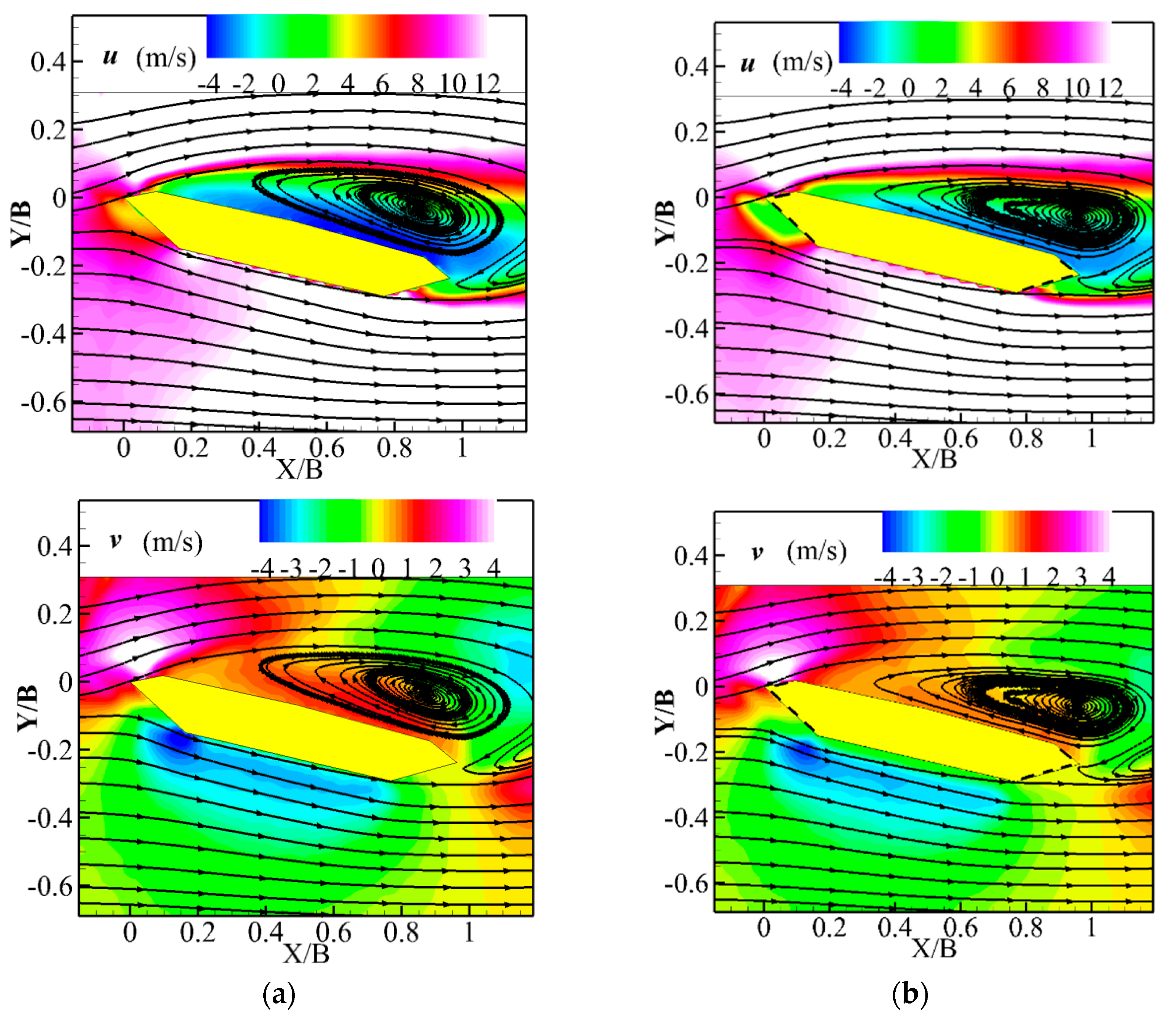
Figure 9 and Figure 10 plot the mean value of u and v distributions around test model. The positive u value denotes an in-flow direction and positive v the upward direction. When the angle of wind attack is −20°, the mean u and v distributions are plotted in Figure 9a,b. It can be seen that the negative u on lower surface and wake flow in Case 4 is smaller than in Case 0, and the positive v on lower surface wake flow in Case 4 is also smaller than in Case 0. This is due to the passive jet formed by Case 4 into the wake. The jet flow interacts with the backward flow and results in a modification to the wake flow of Case 0.
When the wind attack angle is 15°, the mean u and v distributions are plot in Figure 10a,b. It is shown that negative u on upper surface and wake flow in Case 4 is smaller than Case 0, and positive v on upper surface wake flow in Case 4 is also smaller than Case 0. The reason remains the same.
At the wind attack angle of −20°, the instantaneous and time-averaged flow fields are shown in Figure 11. A reverse vortex structure formed on the upper and lower surfaces of the test model of Case 0, which can be seen in Figure 11a. The vortex structure of the upper surface separated from the upper tail of the test model, while the vortex structure of the lower surface separated from the lower leading edge of the test model. The detachment of the unsteady wake vortex structure on the upper and lower surfaces of the model will result in obvious changes in the surface pressure around the model structure. In particular, this happens in the area of flow separation on the lower surface of the test model, as indicated by the surface pressure measurement results given in Figure 7c. For Case 4, the results of the vortex structure around the test model were similar to Case 0, as shown in Figure 11b. However, the vortex strength of Case 4 is lower than that of Case 0, while the wake width is decreased. This is consistent with the fluctuating pressure coefficient distributions, as shown in Figure 7d.
The time-averaged flow fields of both cases are given in Figure 11c,d, respectively. The turbulence kinetic energy (TKE) in the flow fields around the model can be used to indicate the instability of the surface pressure of the bridge model [29], which in turn can represent the instability of the aerodynamic forces in the model. Therefore, TKE values in the flow fields around the test model were used as an indicator to assess the efficiency of the bypass passive jet flow control in this study. It was found that TKE distribution values in the wake of Case 4 are much lower than those in the model without control. Therefore, there will be reduced fluctuations in the aerodynamic forces, which is consistent with the above pressure and aerodynamic measurement results. Moreover, the recirculation region of Case 4 was suppressed to a smaller size.
Figure 12 shows results of the test models at the angle of 15° that are similar to those at the angle of −20°. In comparison with the Case 0 results, TKE values are greatly reduced and the recirculation regions are obviously smaller in size.
As for the two-dimensional incompressible flow, the vorticity in the z direction can be written as:
where x and y are the coordinates along the downstream direction and vertical flow direction. According to Equation (5), both the vortex motion and the shearing motion are identified by the vorticity in the flow, the vortex forming and shedding locations cannot be clearly identified to represent the flow. To get rid of the shearing motions, we used the imaginary part of the complex eigenvalue of the velocity gradient tensor to distinctly visualize vortices [32]. Since the two-dimensional flow velocity fields are obtained through the PIV measurements, the full velocity gradient tensor cannot be formed, and we can only set up a two-dimensional form of the velocity gradient tensor [33] as:
We conducted a detailed experiment focusing on the wake flow behind the test model to investigate the formation of passive jet flow. Here, we adopted swirling strength as the indicator to reveal the jet vortex, as shown in Figure 13a and Figure 14a. It should be noted that the measurement resolution increased to 1.4 mm × 1.4 mm in this case. It can be observed that there are streamlines being evacuated out from the bypass system into the model wake, as shown in Figure 13 and Figure 14.
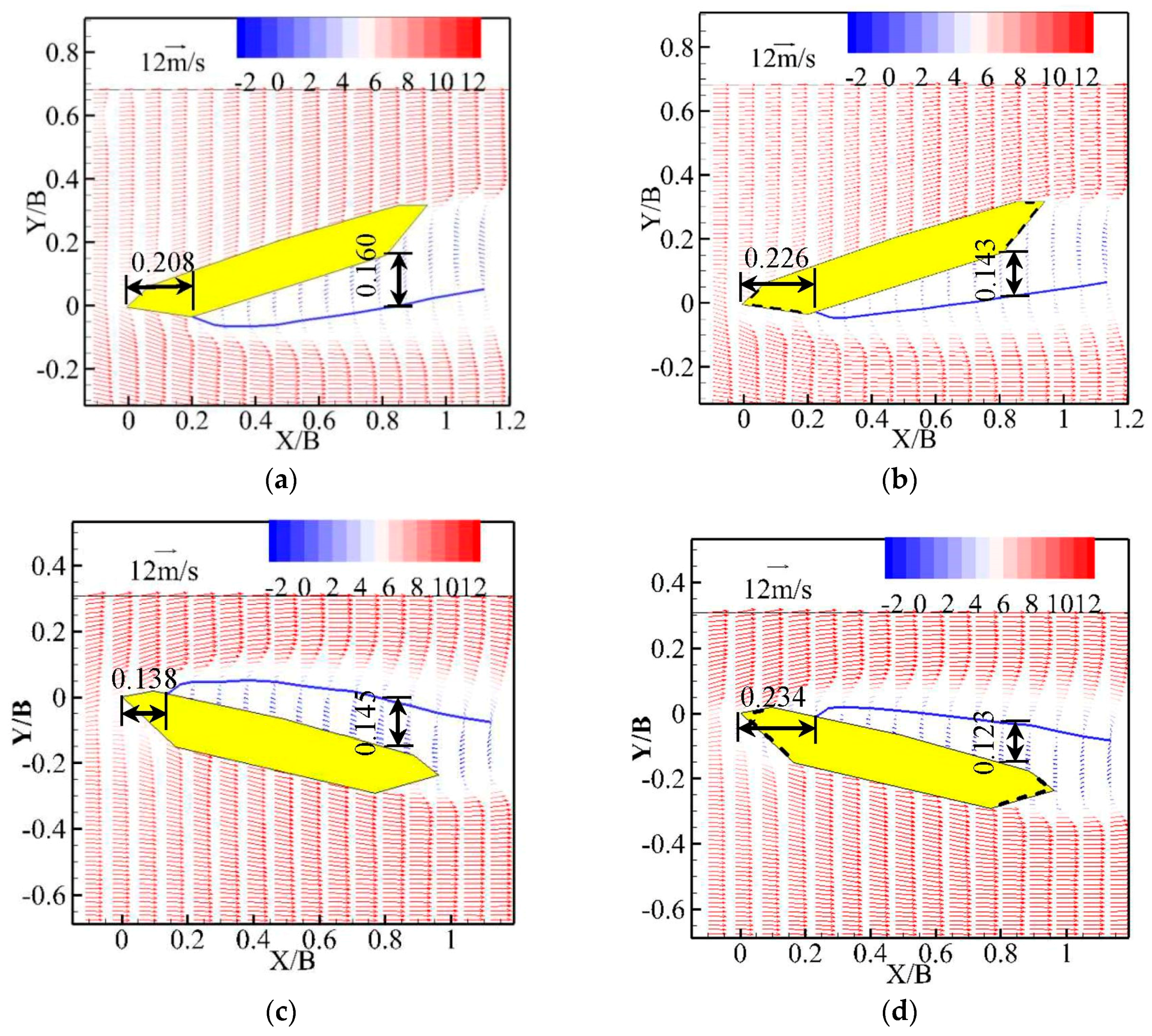
The quantitative analysis of the separation points and the recirculation sizes was then performed, with results shown in Figure 15. The size of the recirculation region is not obvious according the streamlines and vortices; therefore, we conducted an analysis of the velocity profiles near the model surfaces. The blue solid line in Figure 15 in the revised manuscript represents the zero point line of the velocity distribution, and the velocity in the horizontal direction of the position of the model surface separation point is zero. According to these blue lines, we determined the separation points of the flow from the model surfaces. Moreover, the distances between the blue lines and the model surface will reflect the size changes of the recirculation regions. Because 99 × 74 vectors are shown in the fields, the uncertainty may increase by an additional 1/99 × 100% = 1% in the horizontal direction and 1/74 × 100% = 1.4% in the vertical direction under the resolution of PIV measurements. When the wind attack angle was −20°, the flow separation point was X/B = 0.208 away from the leading point for Case 0, while it was delayed to X/B = 0.226 for Case 4. When the wind attack angle was 15°, the flow separation point was X/B = 0.138 for Case 0 before being dramatically pushed down to X/B = 0.234. Then, the recirculation region sizes were quantitatively analyzed when the wind angle was −20°. This quantitative analysis found that the X/B was fixed to 0.8, and the heights of the recirculation regions were 0.160 and 0.143 for Case 0 and Case 4, respectively. The height of the recirculation region was reduced from 0.145 to 0.123 at the angle of 15°. This is consistent with the force and pressure measurement results.
3.4. Discussion of the Results
According to the above analysis of the aerodynamic coefficients, pressure coefficients, and the flow fields around the test models, the present bypass passive jet flow method is effective at different wind attack angles, particularly at larger wind attack angles. It is suggested that this method can achieve a better control effectiveness for the bridge flutter, which will be further investigated in an elastic test model. The model scale is set as 1:125 in the present study, which means that large-scale model tests should be conducted to validate this method in the near future.
The present experimental study has validated the effectiveness of the bypass passive jet flow control on the bridge girder. However, the spacing of the suction/jet holes in the span-wise direction of the single box girder is fixed, and it does not indicate whether the control effect of the present configuration is the best. Therefore, a study focusing on the effects of the spacing ratio is currently being undertaken to facilitate this flow control method being used in engineering applications, and the results will be reported in the near future.
4. Conclusions
In the present study, the control effectiveness of a bypass passive jet flow control on the aerodynamic forces, pressure distributions, and flow field characteristics was examined. Using the connected channels to transport the airflow from the leading side to the trailing side, a good control effectiveness was then achieved by the case with all suction/jet holes on upper and low surfaces opened. Some conclusions were obtained through the present study as follows:
The aerodynamic force measurement results show that the suction/jet holes both set on the upper and lower surfaces are beneficial for control. When the suction/jet holes on the upper and lower surfaces are all opened, the bypass flow control exhibits the best effectiveness.
The pressure distributions indicate that the bypass passive jet flow has less influence on the surface without a flow separation and greater effects on the surface with a flow separation. More opened suction/jet holes can greatly decrease the adverse pressure gradient and fluctuating pressure coefficients.
The flow field characteristics measured by PIV show that the bypass passive jet flow can dramatically decrease the TKE level, delay the flow separation, compress the wake region and reduce the size of the recirculation.
Acknowledgments
This research work is funded by the National Natural Science Foundation of China (NSFC51578188, 51378153, 51008093, 51161120359 and 91215302) and the Fundamental Research Funds for the Central Universities (HIT. BRETIII. 201512).
Author Contributions
W.-L.C. is the project director (PD) and principal investigator (PI). L.-Q.Z., G.-B.C. and W.-L.C. conceived and designed the experiments; L.-Q.Z., G.-B.C. and D.-L.G. performed the experiments. The authors contributed jointly to analyzing the data, discussion and preparing the paper.
Conflicts of Interest
The authors declare no conflict of interest.
References
- Ehsan, F.; Scanlan, R.H. Vortex-induced vibrations of flexible bridges. J. Eng. Mech. 1990, 116, 1392–1411. [Google Scholar] [CrossRef]
- Larsen, A.; Walther, J.H. Aeroelastic analysis of bridge girder sections based on discrete vortex simulations. J. Wind Eng. Ind. Aerodyn. 1997, 67, 253–265. [Google Scholar] [CrossRef]
- Larsen, A. Advances in aeroelastic analyses of suspension and cable-stayed bridges. J. Wind Eng. Ind. Aerodyn. 1998, 74–76, 73–90. [Google Scholar] [CrossRef]
- Taylor, Z.J.; Gurka, R.; Kopp, G.A. Geometric effects on shedding frequency for bridge sections. In Proceedings of the 11th Americas conference on wind engineering, San Juan, Puerto Rico, 22–26 June 2009. [Google Scholar]
- Larsen, A.; Esdahl, S.; Andersen, J.E.; Vejrum, T. Storebaelt suspension bridge-vortex shedding excitation and mitigation by guide vanes. J. Wind Eng. Ind. Aerodyn. 2000, 88, 283–296. [Google Scholar] [CrossRef]
- Fujino, Y.; Yoshitaka, Y. Wind-induced vibration and control of Trans-Tokyo Bay Crossing Bridge. J. Struct. Eng. 2002, 128, 1012–1025. [Google Scholar] [CrossRef]
- Li, H.; Laima, S.J.; Ou, J.P.; Zhao, X.F.; Zhou, W.S.; Yu, Y.; Li, N.; Liu, Z.Q. Investigation of vortex-induced vibration of a suspension bridge with two separated steel box girders based on field measurements. Eng. Struct. 2011, 33, 1894–1907. [Google Scholar] [CrossRef]
- Larsen, A.; Svensson, E.; Andersen, H. Design aspects of tuned mass dampers for the Great Belt East Bridge approach spans. J. Wind Eng. Ind. Aerodyn. 1995, 54–55, 413–426. [Google Scholar] [CrossRef]
- Andersen, L.; Birch, N.W.; Hansen, A.H.; Skibelund, J.O. Response analysis of tuned mass dampers to structures exposed to vortex loading of Simiu-Scanlan Type. J. Sound. Vib. 2001, 239, 217–231. [Google Scholar] [CrossRef]
- Battista, R.C.; Pfeil, M.S. Reduction of vortex-induced oscillations of Rio–Niterói Bridge by dynamic control devices. J. Wind Eng. Ind. Aerodyn. 2000, 84, 273–288. [Google Scholar] [CrossRef]
- Zhang, H.F.; Xin, D.B.; Ou, J.P. Wake control of vortex shedding based on spanwise suction of a bridge section model using Delayed Detached Eddy Simulation. J. Wind Eng. Ind. Aerodyn. 2016, 155, 100–114. [Google Scholar] [CrossRef]
- Bakis, K.N.; Massaro, M.; Williams, M.S.; Limebeer, D.J.N. Aeroelastic control of long-span suspension bridges with controllable winglets. Struct. Control Health Monit. 2016, 23, 1417–1441. [Google Scholar] [CrossRef]
- Wang, Q.; Liao, H.L.; Li, M.S.; Ma, C. Influence of aerodynamic configuration of a streamline box girder on bridge flutter and vortex-induced vibration. J. Mod. Transp. 2011, 19, 261–267. [Google Scholar] [CrossRef]
- Bruno, L.; Mancini, G. Importance of Deck Details in Bridge Aerodynamics. Struct. Eng. Int. 2002, 12, 289–294. [Google Scholar] [CrossRef]
- Zhou, R.; Yang, Y.X.; Ge, Y.J.; Priyan, M.; Damith, M. Practical countermeasures for the aerodynamic performance of long-span cable-stayed bridges with open decks. Wind Struct. 2015, 21, 223–239. [Google Scholar] [CrossRef]
- El-Gammal, M.; Hangan, H.; King, P. Control of vortex shedding-induced effects in a sectional bridge model by spanwise perturbation method. J. Wind Eng. Ind. Aerodyn. 2007, 95, 663–678. [Google Scholar] [CrossRef]
- Baek, H.; Karniadakis, G.E. Suppressing vortex-induced vibrations via passive means. J. Fluid Struct. 2009, 25, 848–866. [Google Scholar] [CrossRef]
- Chen, W.L.; Gao, D.L.; Yuan, W.Y.; Li, H.; Hu, H. Passive jet control of flow around a circular cylinder. Exp. Fluids 2015, 56, 201. [Google Scholar] [CrossRef]
- Larose, G.L.; D’Auteuil, A. On the Reynolds number sensitivity of the aerodynamics of bluff bodies with sharp edges. J. Wind Eng. Ind. Aerodyn. 2006, 94, 365–376. [Google Scholar] [CrossRef]
- Larsen, A.; Savage, M.; Lafrenière, A.; Hui, M.C.H.; Lansen, S.V. Investigation of vortex response of a twin box bridge section at high and low Reynolds numbers. J. Wind Eng. Ind. Aerodyn. 2008, 96, 934–944. [Google Scholar] [CrossRef]
- Li, H.; Laima, S.J.; Jing, H. Reynolds number effects on aerodynamic characteristics and vortex-induced vibration of a twin-box girder. J. Fluid Struct. 2014, 50, 358–375. [Google Scholar] [CrossRef]
- Irwin, H.P.A.H.; Cooper, K.R.; Girard, R. Correction of distortion effects caused by tubing systems in measurements of fluctuating pressures. J. Wind Eng. Ind. Aerodyn. 1979, 5, 93–107. [Google Scholar] [CrossRef]
- Barlow, B.; Rae, H.; Pope, A. Low-Speed Wind Tunnel Testing, 3rd ed.; Wiley: New York, NY, USA, 1999; pp. 330–375. [Google Scholar]
- Hu, H.; Koochesfahani, M.M. Thermal Effects on the Wake of a Heated Circular Cylinder Operating in Mixed Convection Regime. J. Fluid Mech. 2011, 685, 235–270. [Google Scholar] [CrossRef]
- Liu, Y.; Chen, W.L.; Bond, L.; Hu, H. An Experimental Study on the Characteristics of Wind-driven Surface Water Film Flows by Using a Multi-Transducer Ultrasonic Pulse-Echo Technique. Phys. Fluids 2017, 29, 012102. [Google Scholar] [CrossRef]
- Tian, W.; Ozbay, A.; Hu, H. Effects of Incoming Surface Wind Conditions on the Wake Characteristics and Dynamic Wind Loads Acting on a Wind Turbine Model. Phys. Fluids 2014, 26, 125108. [Google Scholar] [CrossRef]
- Yuan, W.Y.; Laima, S.J.; Chen, W.L.; Li, H.; Hu, H. Investigation on the vortex-and-wake-induced vbiration of a separated-box bridge girder. J. Fluid Struct. 2017, 70, 145–161. [Google Scholar] [CrossRef]
- Samimy, M.; Lele, S.K. Motion of particles with inertia in a compressible free shear layer. Phys. Fluids 1991, 3, 1915–1923. [Google Scholar] [CrossRef]
- Chen, W.L.; Li, H.; Hu, H. An experimental study on a suction flow control method to reduce the unsteadiness of the wind loads acting on a circular cylinder. Exp. Fluids 2014, 55, 1707. [Google Scholar] [CrossRef]
- Frandsen, J.B. Comparison of numerical prediction and full-scale measurements of vortex induced oscillations. In Proceedings of the 4th International Colloquium on Bluff Body Aerodynamics and Applications, Ruhu-University of Bochum, Bochum, Germany, 11–14 September 2000. [Google Scholar]
- Gao, D.L.; Chen, W.L.; Li, H.; Hu, H. Flow around a circular cylinder with slit. Exp. Therm. Fluid Sci. 2017, 82, 287–301. [Google Scholar] [CrossRef]
- Zhou, J.; Adrian, R.J.; Balachandar, S.; Kendall, T.M. Mechanisms for generating coherent packets of hairpin vortices in channel flow. J. Fluid Mech. 1999, 387, 353–396. [Google Scholar] [CrossRef]
- Chen, W.L.; Li, H.; Hu, H. An experimental study on the unsteady vortices and turbulent flow structures around twin-box-girder bridge deck models with different gap ratios. J. Wind Eng. Ind. Aerodyn. 2014, 132, 27–36. [Google Scholar] [CrossRef]
Figure 1.
A sketch view of the test section.

Figure 2.
Geometry information of the cross-section of the segment models and five control schemes (unit: mm). (a) Case 0; (b) Case 1; (c) Case 2; (d) Case 3; (e) Case 4; (f) Case 5.
Figure 2.
Geometry information of the cross-section of the segment models and five control schemes (unit: mm). (a) Case 0; (b) Case 1; (c) Case 2; (d) Case 3; (e) Case 4; (f) Case 5.
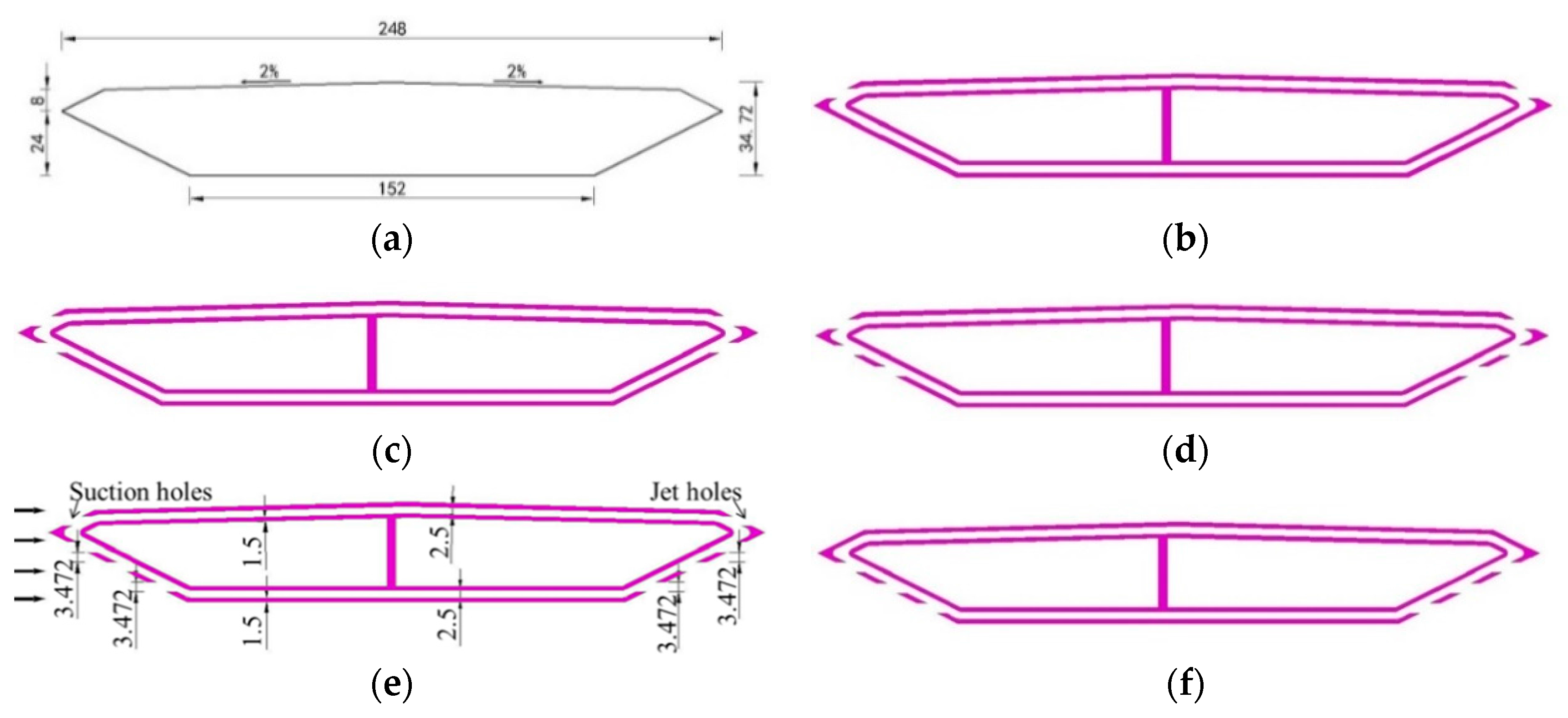
Figure 3.
View of the model from the downstream direction.

Figure 4.
The distribution of pressure measurement taps.
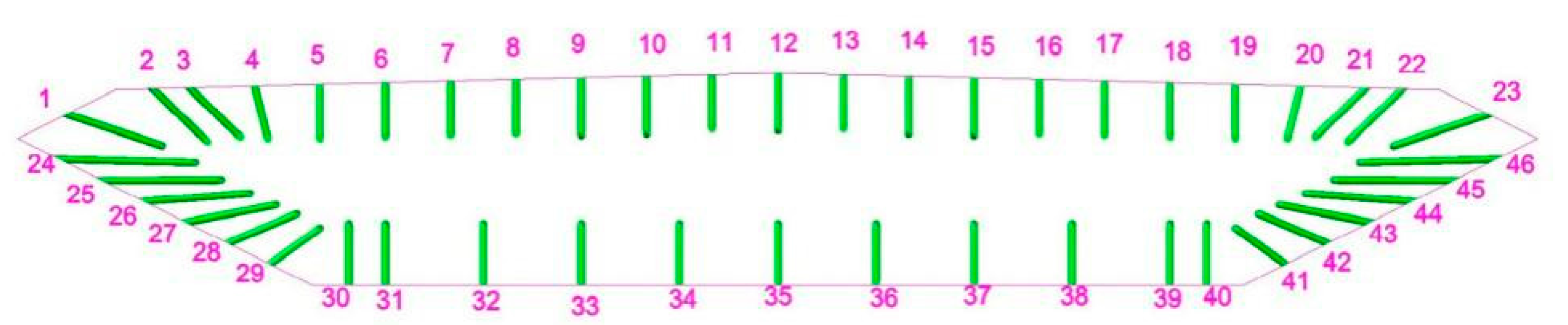
Figure 5.
Comparison of mean aerodynamic force coefficients between five control cases and Case 0 at different wind attack angles. (a) Cl_mean; (b) Cd_mean; (c) Cm_mean.
Figure 5.
Comparison of mean aerodynamic force coefficients between five control cases and Case 0 at different wind attack angles. (a) Cl_mean; (b) Cd_mean; (c) Cm_mean.
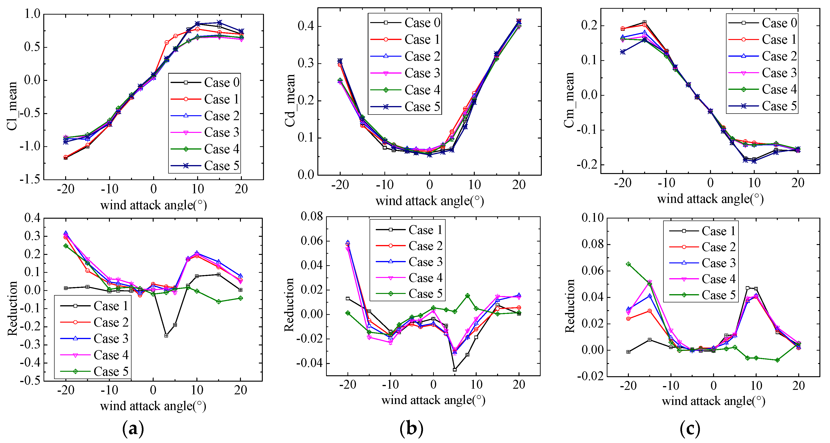
Figure 6.
Comparison of aerodynamic force coefficient fluctuations between five control cases and Case 0 at different wind attack angles. (a) Cl_rms; (b) Cd_rms; (c) Cm_rms.
Figure 6.
Comparison of aerodynamic force coefficient fluctuations between five control cases and Case 0 at different wind attack angles. (a) Cl_rms; (b) Cd_rms; (c) Cm_rms.
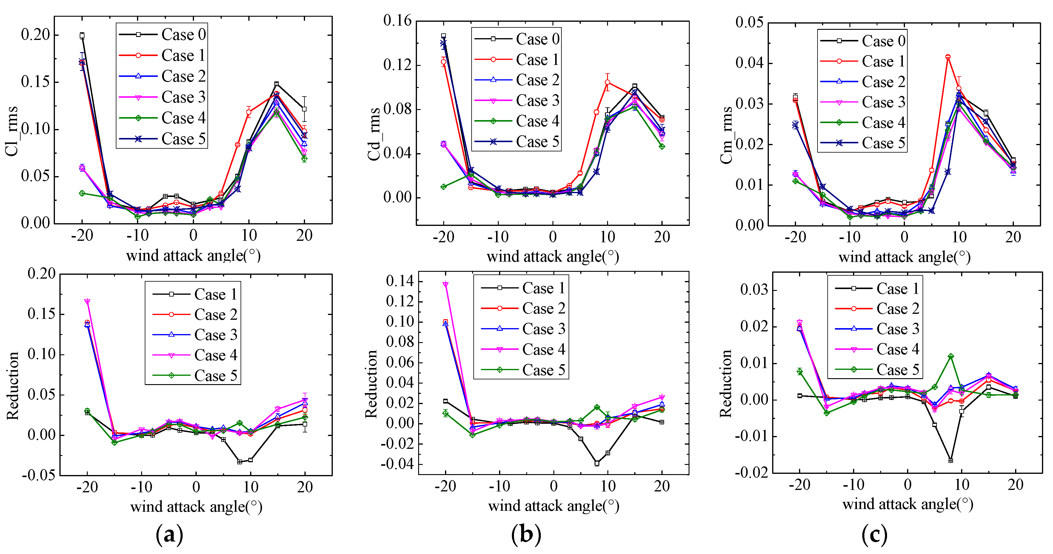
Figure 7.
Distributions of mean and RMS (root-mean-square) values of pressure coefficients at the wind attack angle of −20°: (a,b) are the upper surface and (c,d) are the lower surface.
Figure 7.
Distributions of mean and RMS (root-mean-square) values of pressure coefficients at the wind attack angle of −20°: (a,b) are the upper surface and (c,d) are the lower surface.
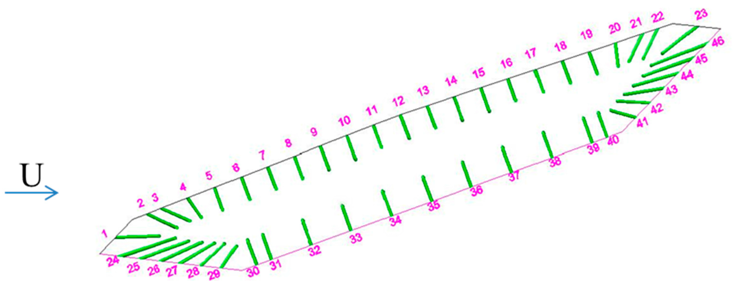
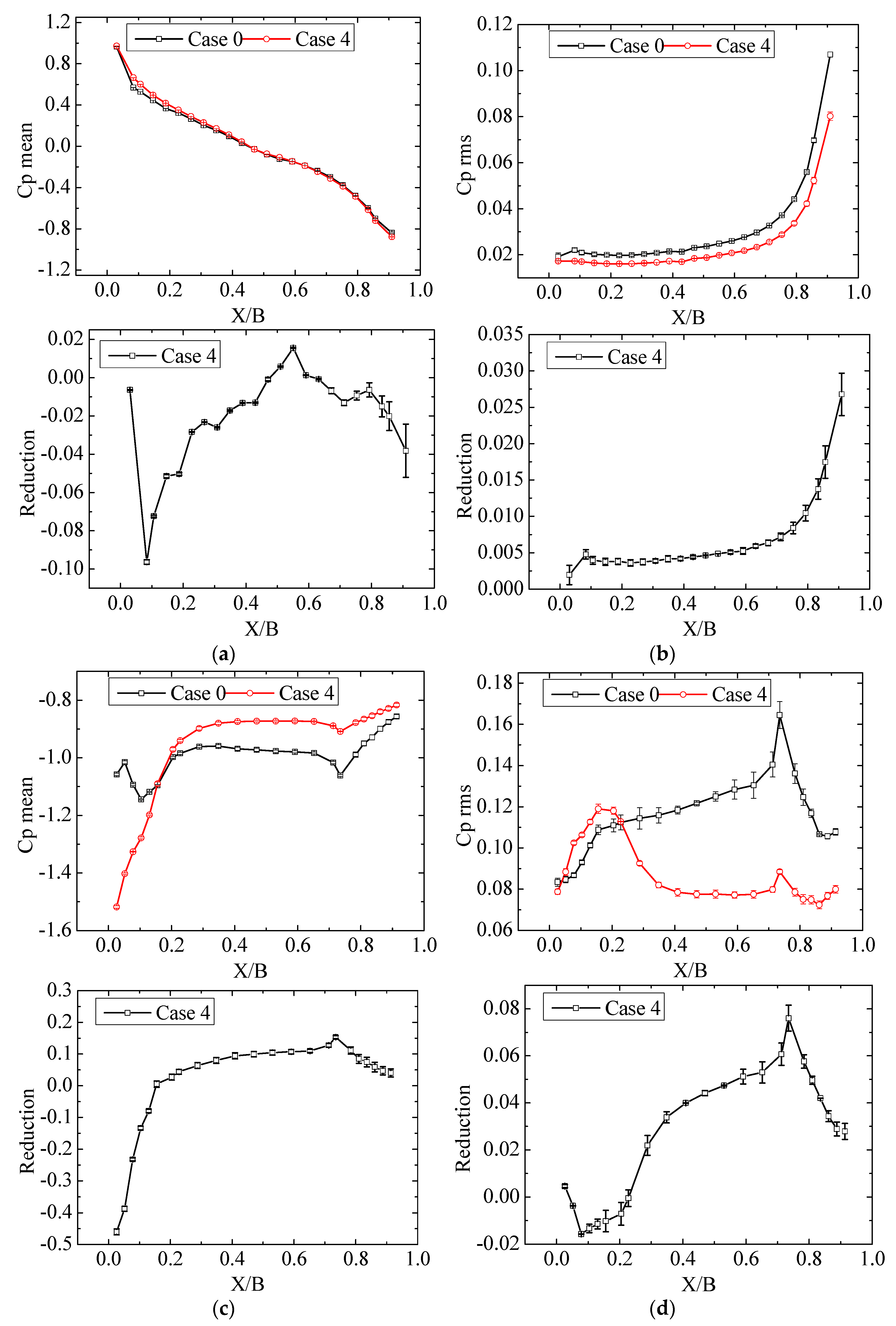
Figure 8.
Distributions of mean and RMS values of pressure coefficient at the wind attack angle of 15°: (a,b) are the upper surface and (c,d) are the lower surface.
Figure 8.
Distributions of mean and RMS values of pressure coefficient at the wind attack angle of 15°: (a,b) are the upper surface and (c,d) are the lower surface.


Figure 9.
The particle imaging velocimetry (PIV) measurement results for Case 0 and by-pass jet control at wind attack angle of −20°. (a) Case 0; (b) Case 4.
Figure 9.
The particle imaging velocimetry (PIV) measurement results for Case 0 and by-pass jet control at wind attack angle of −20°. (a) Case 0; (b) Case 4.
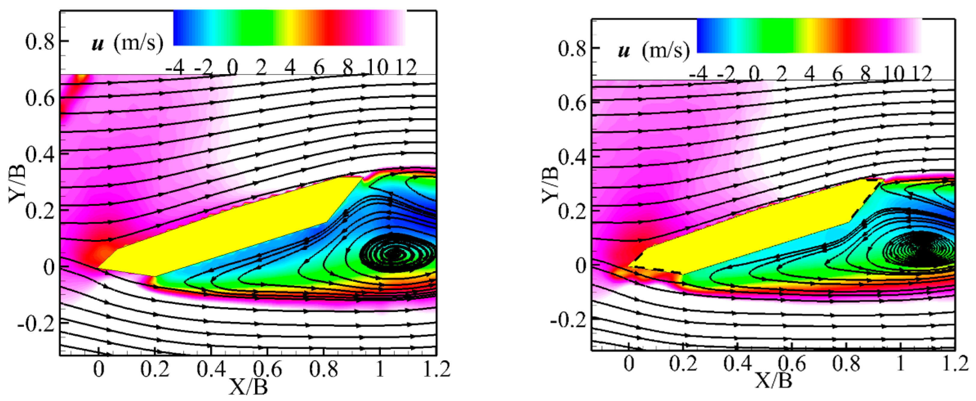
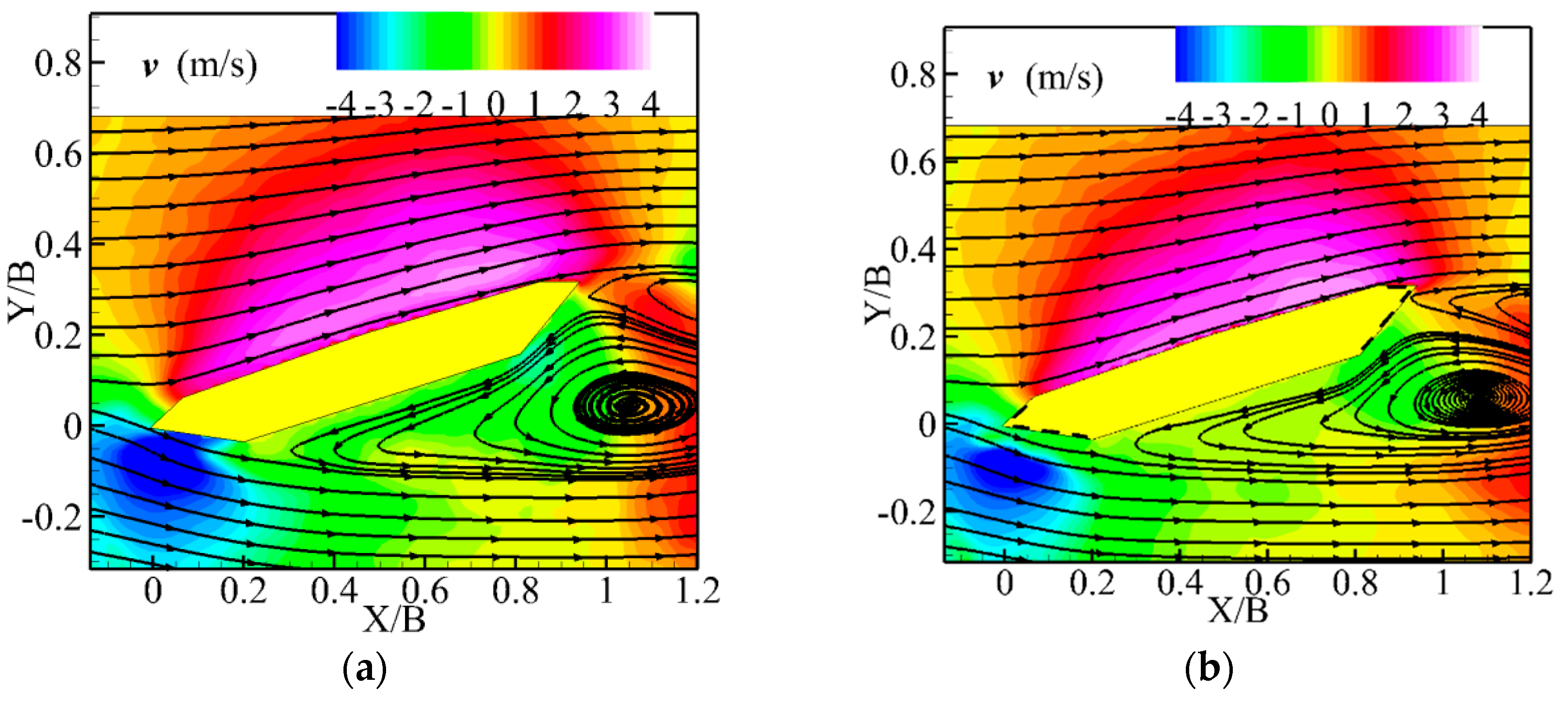
Figure 10.
The PIV measurement results for Case 0 and by-pass jet control at wind attack angle of 15°. (a) Case 0; (b) Case 4.
Figure 10.
The PIV measurement results for Case 0 and by-pass jet control at wind attack angle of 15°. (a) Case 0; (b) Case 4.

Figure 11.
The PIV measurement results for Case 0 and bypass jet control at a wind attack angle of −20°. (a) Instantaneous flow field of Case 0; (b) Instantaneous flow field of Case 4; (c) Time-averaged flow field of Case 0; (d) Time-averaged flow field of Case 4. TKE: turbulence kinetic energy.
Figure 11.
The PIV measurement results for Case 0 and bypass jet control at a wind attack angle of −20°. (a) Instantaneous flow field of Case 0; (b) Instantaneous flow field of Case 4; (c) Time-averaged flow field of Case 0; (d) Time-averaged flow field of Case 4. TKE: turbulence kinetic energy.
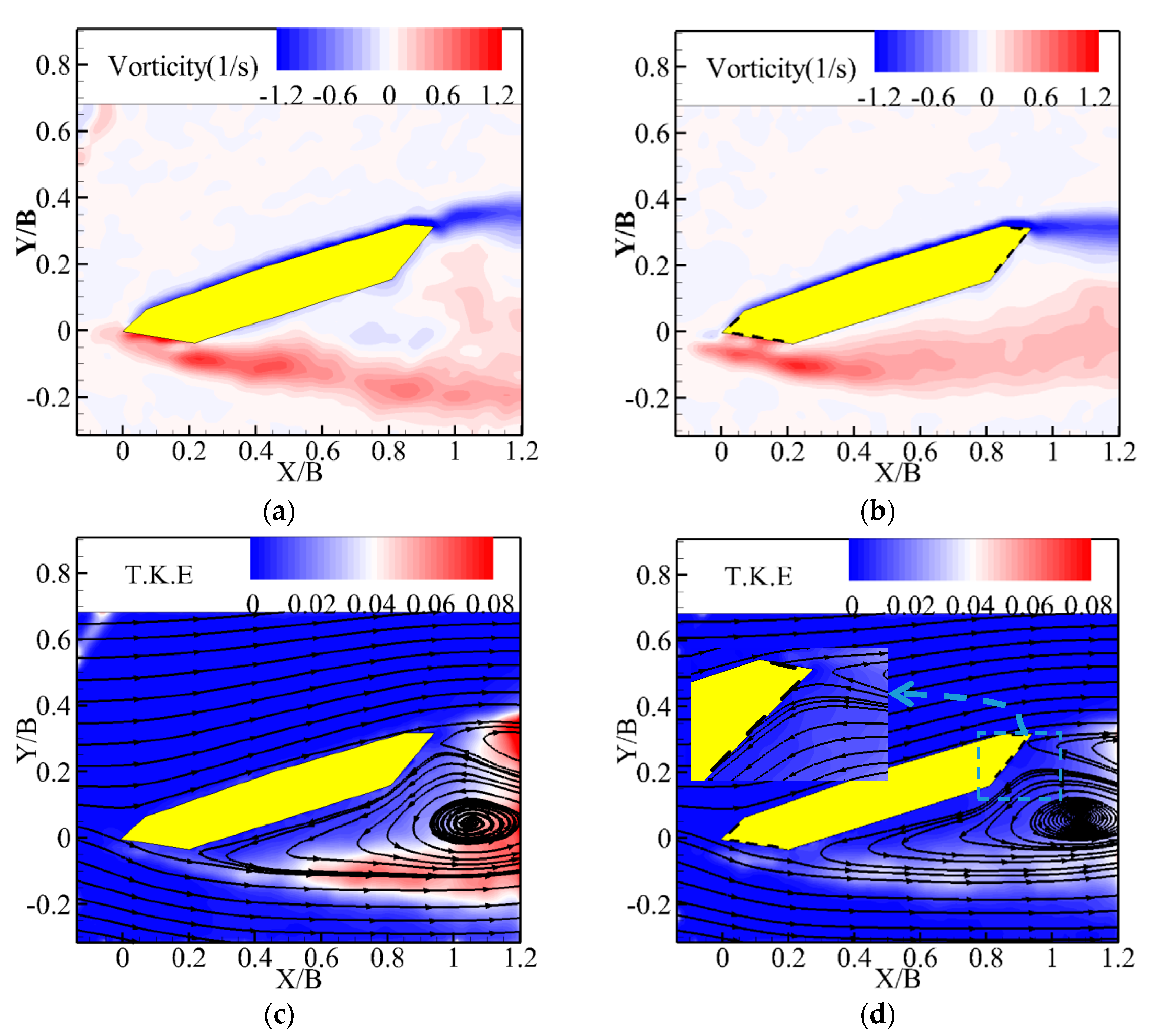
Figure 12.
Instantaneous and time-averaged flow fields for Case 0 and bypass jet control at a wind attack angle of 15°. (a) Instantaneous flow field of Case 0; (b) Instantaneous flow field of Case 4; (c) Time-averaged flow field of Case 0; (d) Time-averaged flow field of Case 4.
Figure 12.
Instantaneous and time-averaged flow fields for Case 0 and bypass jet control at a wind attack angle of 15°. (a) Instantaneous flow field of Case 0; (b) Instantaneous flow field of Case 4; (c) Time-averaged flow field of Case 0; (d) Time-averaged flow field of Case 4.
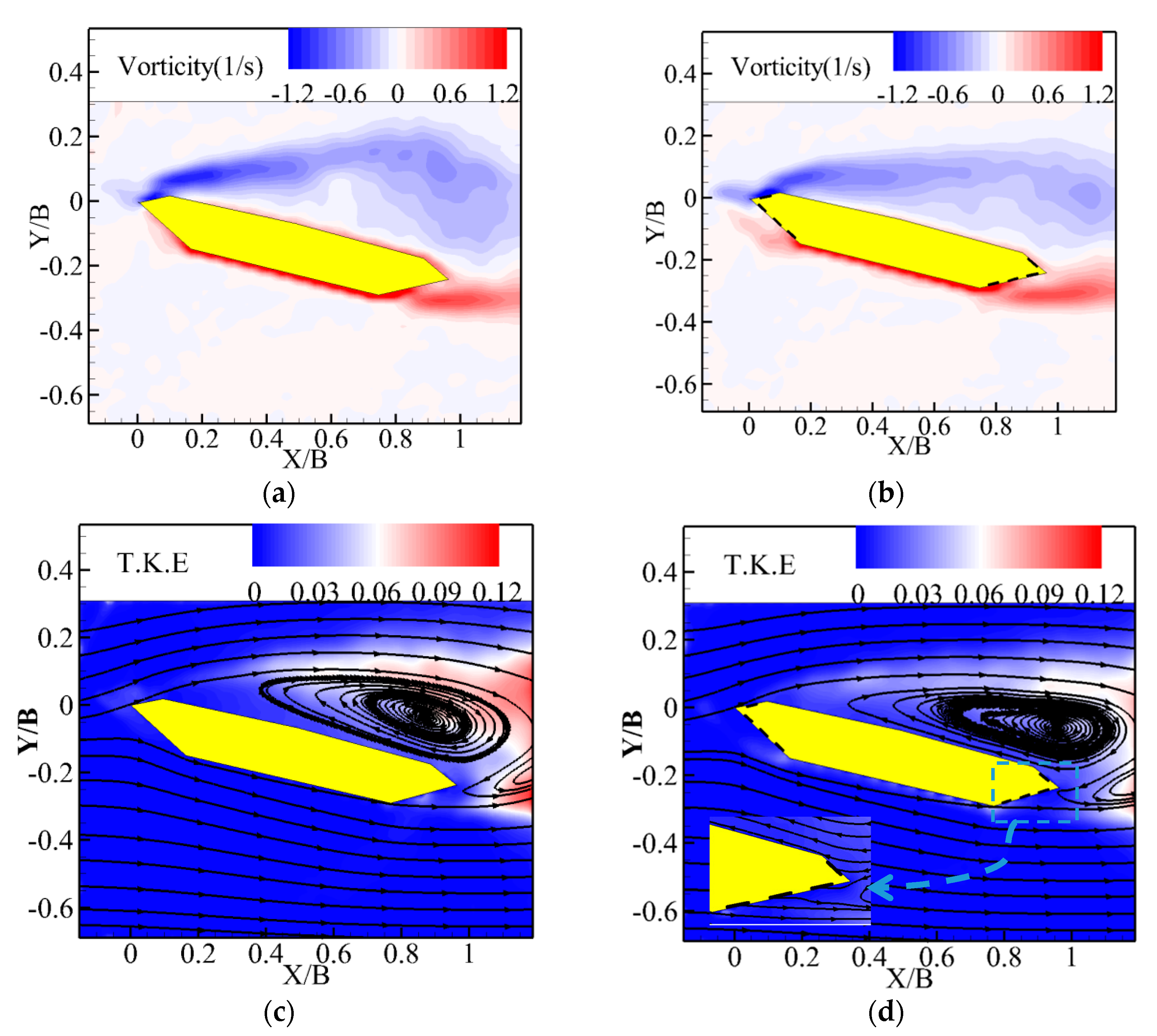
Figure 13.
The instantaneous and time-averaged flow fields for the by-pass jet control at wind attack angle of 15°. (a) Instantaneous flow field of Case 4; (b) Time-averaged flow field of Case 4.
Figure 13.
The instantaneous and time-averaged flow fields for the by-pass jet control at wind attack angle of 15°. (a) Instantaneous flow field of Case 4; (b) Time-averaged flow field of Case 4.
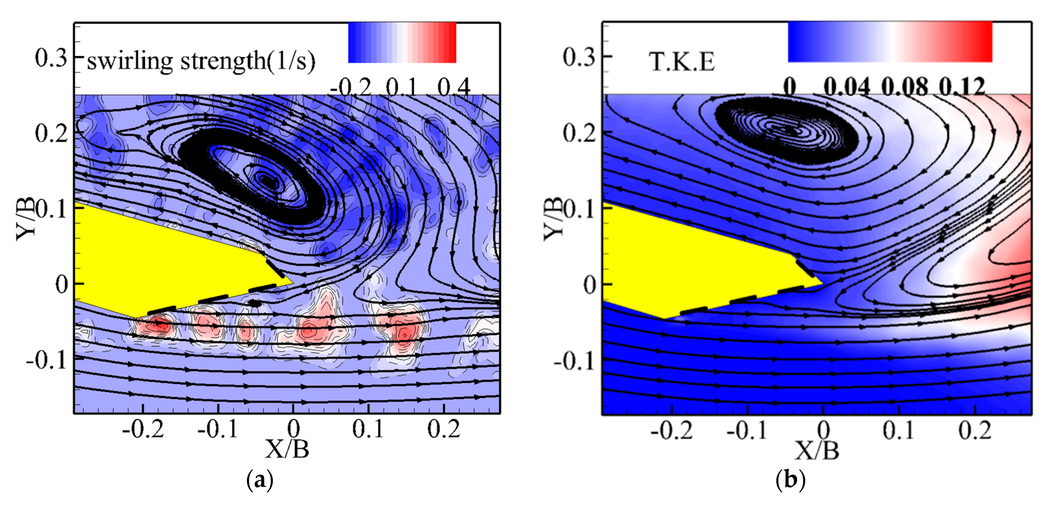
Figure 14.
The instantaneous and time-averaged flow fields for the by-pass jet control at wind attack angle of −20°. (a) Instantaneous flow field of Case 4; (b) Time-averaged flow field of Case 4.
Figure 14.
The instantaneous and time-averaged flow fields for the by-pass jet control at wind attack angle of −20°. (a) Instantaneous flow field of Case 4; (b) Time-averaged flow field of Case 4.
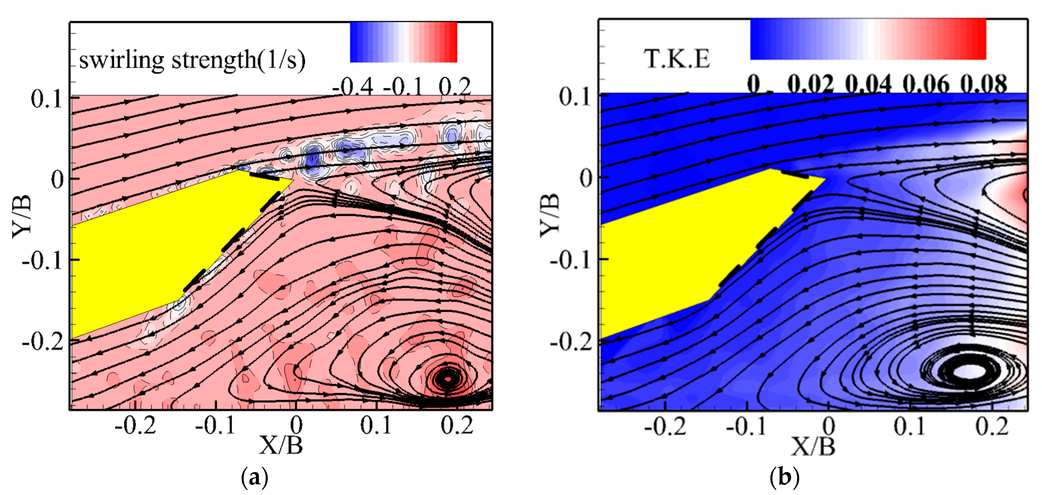
Figure 15.
Velocity profiles for the Case 0 and bypass jet control. (a) Case 0 at wind attack angle −20°; (b) Case 4 at wind attack angle −20°; (c) Case 0 at wind attack angle 15°; (d) Case 4 at wind attack angle 15°.
Figure 15.
Velocity profiles for the Case 0 and bypass jet control. (a) Case 0 at wind attack angle −20°; (b) Case 4 at wind attack angle −20°; (c) Case 0 at wind attack angle 15°; (d) Case 4 at wind attack angle 15°.


Table 1.
Control schemes of the test models.
| Control Case | Suction/Jet Holes on US | First Row of Suction/Jet Holes on LS | Second Row of Suction/Jet Holes on LS | Third Row of Suction/Jet Holes on LS | Jsuc |
|---|---|---|---|---|---|
| Case 0 | closed | closed | closed | closed | 0 |
| Case 1 | open | closed | closed | closed | 0.0667 |
| Case 2 | open | open | closed | closed | 0.1333 |
| Case 3 | open | open | open | closed | 0.2000 |
| Case 4 | open | open | open | open | 0.2667 |
| Case 5 | closed | open | open | open | 0.2000 |
Note: US = upper surface and LS = lower surface.
Table 2.
Integral of Cm_mean along the wind attack angle.
| Control Case | Case 0 | Case 1 | Case 2 | Case 3 | Case 4 | Case 5 |
|---|---|---|---|---|---|---|
| Cm_mean * (attack angle) | 5.26 ± 0.017 | 4.80 ± 0.003 | 4.65 ± 0.007 | 4.58 ± 0.006 | 4.48 ± 0.004 | 4.88 ± 0.002 |
* Cm_mean (attack angle) is the integral of Cm_mean along the wind attack angle.
© 2017 by the authors. Licensee MDPI, Basel, Switzerland. This article is an open access article distributed under the terms and conditions of the Creative Commons Attribution (CC BY) license (http://creativecommons.org/licenses/by/4.0/).
Share and Cite
MDPI and ACS Style
Zhang, L.-Q.; Chen, G.-B.; Chen, W.-L.; Gao, D.-L. Separation Control on a Bridge Box Girder Using a Bypass Passive Jet Flow. Appl. Sci. 2017, 7, 501. https://doi.org/10.3390/app7060501
AMA Style
Zhang L-Q, Chen G-B, Chen W-L, Gao D-L. Separation Control on a Bridge Box Girder Using a Bypass Passive Jet Flow. Applied Sciences. 2017; 7(6):501. https://doi.org/10.3390/app7060501
Chicago/Turabian StyleZhang, Liang-Quan, Guan-Bin Chen, Wen-Li Chen, and Dong-Lai Gao. 2017. "Separation Control on a Bridge Box Girder Using a Bypass Passive Jet Flow" Applied Sciences 7, no. 6: 501. https://doi.org/10.3390/app7060501
Note that from the first issue of 2016, this journal uses article numbers instead of page numbers. See further details here.