
Low Frequency Interactive Auralization Based on a Plane Wave Expansion


Institute of Sound and Vibration Research, University of Southampton, SO17 1BJ, UK
*
Author to whom correspondence should be addressed.
†
Current address: Faculty of Engineering, Universidad de San Buenaventura Medellín, Cra 56C No 51-110, 050010 Medellín, Colombia.
Appl. Sci. 2017, 7(6), 558; https://doi.org/10.3390/app7060558
Submission received: 2 March 2017
/
Revised: 12 May 2017
/
Accepted: 23 May 2017
/
Published: 27 May 2017
(This article belongs to the Special Issue Spatial Audio)
Abstract
:This paper addresses the problem of interactive auralization of enclosures based on a finite superposition of plane waves. For this, room acoustic simulations are performed using the Finite Element (FE) method. From the FE solution, a virtual microphone array is created and an inverse method is implemented to estimate the complex amplitudes of the plane waves. The effects of Tikhonov regularization are also considered in the formulation of the inverse problem, which leads to a more efficient solution in terms of the energy used to reconstruct the acoustic field. Based on this sound field representation, translation and rotation operators are derived enabling the listener to move within the enclosure and listen to the changes in the acoustic field. An implementation of an auralization system based on the proposed methodology is presented. The results suggest that the plane wave expansion is a suitable approach to synthesize sound fields. Its advantage lies in the possibility that it offers to implement several sound reproduction techniques for auralization applications. Furthermore, features such as translation and rotation of the acoustic field make it convenient for interactive acoustic renderings.
1. Introduction
Auralization is a subject of great interest in different areas because it enables the generation of an audible perception of the acoustic properties of a specific environment [1]. It is a powerful technique because it allows the sound field to be rendered according to the characteristics of the medium, which has applications in the evaluation and understanding of the physical phenomenon under consideration. For room acoustics, auralization provides a convenient tool for experimental tests, subjective evaluations, virtual reality and architectural design.
A significant feature that enhances the auralization technique is the generation of interactive environments in which the listener can move within the enclosure. This is achieved by synthesizing the acoustic field in real time according to the properties of the room and the source-receiver paths. Several approaches have been proposed in the scientific literature to generate interactive auralizations based on Geometrical Acoustics (GA) [2,3,4,5,6]. Nevertheless, at low frequencies, the assumptions required for GA are not generally satisfied, which requires the use of different techniques, such as the numerical solution of the wave equation. The Finite Element Method (FEM) [7], the Boundary Element Method (BEM) [8] and the Finite Difference Time Domain (FDTD) method [9] are some of the techniques commonly used to estimate room impulse responses. However, the computational cost required by these approaches to predict the solution constrains their use for real-time applications.
Despite the significant computational cost of the above methods, some alternatives have been formulated to generate interactive environments based on wave propagation. Mehra et al. proposed the use of the equivalent source method for the rendering of acoustic fields of large and open scenes in real time [10]. Although the approach allows for the reconstruction of the sound field in real time, limitations related to static sound sources or the inclusion of the Doppler effect have to be overcome. The inclusion of the directivity of sound sources and listeners using a spherical harmonic representation has also been proposed by the same author to extend the versatility of the methodology [11]. Another approach proposed by Raghuvanshi [12] simulates the synthesis and propagation of sound. The solution method, denoted as Adaptive Rectangular Decomposition (ARD), permits real-time computation providing a platform for interactive auralizations. The main advantages of the method are the use of dynamic listener/sources and its ability to simulate large complex 3D scenes. Alternatively, Savioja presented a different strategy to predict acoustic fields in real time [13]. The numerical solver corresponds to an FDTD model running over GPUs using parallel computing techniques. The results indicate that this methodology allows the simulation up to 1.5 kHz in moderate size domains. Dynamic listener and multiple sources are also possible based on this processing scheme.
A different approach to interactive auralizations based on the numerical solution of the wave equation is to encode spatial information from the predicted acoustic pressure data. Translation and rotation of the acoustic field can be then achieved by the application of mathematical operators. Southern et al. [14] proposed a method to obtain a spherical harmonic representation of FDTD simulations. The approach uses the the Blumlein difference technique to create a higher order directivity pattern from two adjacent lower orders. This is achieved by approximating the gradient of the pressure as the difference between two neighbouring pressure points on the grid where the solution was computed. The rotation of the acoustic field can be easily computed by a rotation matrix, whereas the translation can be recreated by an interpolation process between spatial impulse responses [15]. Sheaffer et al. [16] suggested the formulation of an inverse problem to generate a spherical harmonic representation of acoustic fields predicted using FDTD. A binaural rendering is achieved based on the relation between spherical harmonics, plane waves and HRTFs.
An implementation of a Plane Wave Expansion (PWE) is carried out in the current study as an alternative methodology to generate an interactive auralization from predicted acoustic numerical data. The methodology has been evaluated by using FE results, but can readily be implemented using other numerical methods. The approach is based on the concept that the acoustic pressure at each node of the mesh can be understood as the output of a virtual omnidirectional microphone. By using the data from the mesh, it is possible to create a virtual microphone array, which, with the implementation of an inverse method, allows for the estimation of complex amplitudes of a set of plane waves that synthesize the desired acoustic field. The use of an inverse method to generate a plane wave expansion from predicted pressure data was previously studied by Støfringsdal and Svensson for 2D cases [17]. An extension of their work is presented in this paper to the 3D case.
Based on a plane wave representation, mathematical operators can be implemented to enable interactive features for auralization applications. The translational movement of the listener can be generated by the translation of the plane wave expansion [18,19]. In terms of the listener’s rotation, a spherical harmonic transformation can be used to rotate the acoustic field [20]. A rotation in the plane wave domain is achieved by the implementation of a VBAP algorithm. Nevertheless, experiments conducted by Murillo [21] suggest that the spherical harmonic transformation is more accurate for this specific application.
A complete framework for an interactive auralization based on a plane wave representation is presented in this article. The processing chain involves the use of an inverse method to extract spatial information from FE simulations, the use of translation and rotation operators, the combination of real-time audio processing with a visual interface and binaural rendering to reproduce the acoustic field. The proposed approach is evaluated by testing it within a real-time auralization system as a reference case. This auralization system allows us to emulate interactively wave phenomena, such as the modal behaviour of the enclosure or acoustic diffraction. The remaining parts of the paper are organized as follows: The mathematical foundations of the plane wave expansion and the derivation of the translation and rotation operators are reviewed in Section 2. The implementation of an inverse method to generate a plane wave representation of the predicted acoustic fields is presented in Section 3. In Section 4, a real-time auralization system is developed, which allows for the evaluation of the proposed approach. The discussion and evaluation of the results are considered in Section 5. Finally, conclusions of the current work are presented in Section 6.
2. Mathematical Foundations
A particular solution of the homogeneous Helmholtz equation for a singular radian frequency is given by a complex pressure field , which corresponds to a plane wave arriving in the direction of a unit vector with an arbitrary complex amplitude q and wavenumber k. The vector identifies the position where the acoustic pressure is evaluated, and the symbol “·” represents the scalar product operation. The plane wave approximation is appropriate at a large distance from the acoustic source, where the curvature of the wave can be ignored. In a similar way, an acoustic field that satisfies the homogeneous Helmholtz equation can be represented by means of a Plane Wave Expansion (PWE) as:
in which is the evaluation point, indicates the different incoming directions of the plane waves, is the amplitude density function and is the unitary sphere [19]. The synthesis of acoustic fields based on a plane wave representation is a common approach [16,17] being adaptable to several audio reproduction techniques. Binaural reproduction is performed by the convolution of the plane waves with the HRTFs according to the direction of arrival [22]. The relation and transformation between the PWE, Ambisonics and wave field synthesis are presented in [23]. Furthermore, mathematical operators to translate [18,19] and rotate [20] the acoustic field are available, which makes this sound field representation convenient for interactive applications. The disadvantage of this method is that the assumption of plane waves makes the approach suitable for sound fields generated by sources located at a large distance from the listener. In addition, the implementation of an infinite number of plane waves is not feasible, and the use of discrete wave directions generates artefacts in the sound field reconstruction.
2.1. Translation of the Acoustic Field
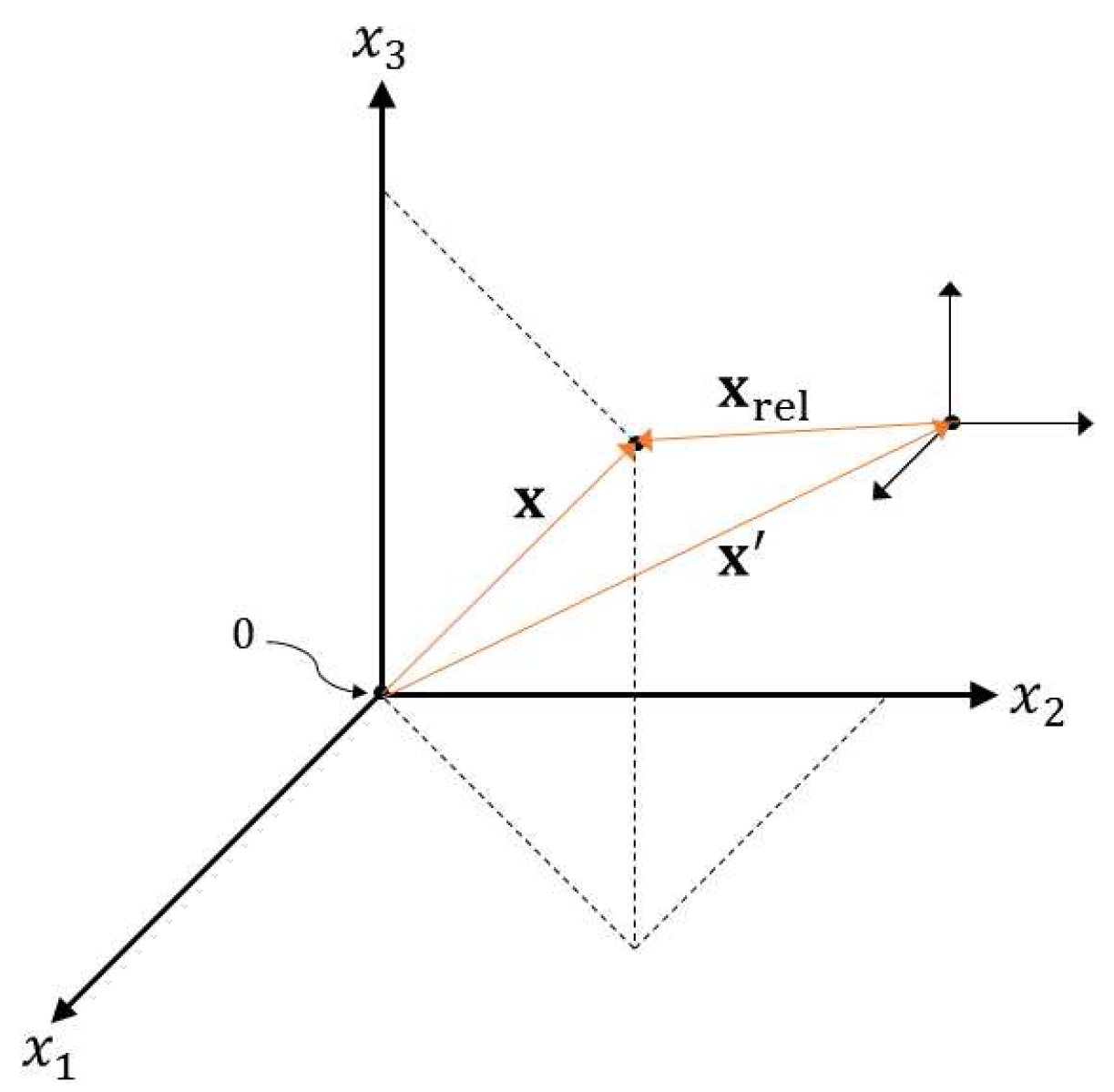
Figure 1 shows the vector , which identifies the origin of a relative coordinate system corresponding to the centre of the listener’s head. The vector defines the same point in space in the relative coordinate system as is identified by the vector in absolute coordinates.
The sound field translation operator is derived by considering two plane wave expansions of the same sound field, but centred at different points in space, specifically at the origin of the absolute and relative coordinate systems. In this case, the difference between the two plane wave expansions is given by the plane wave amplitude densities and , respectively. Therefore, the objective is to express one density in terms of the other. This is achieved by expanding as , leading to:
Equation (2) indicates that is the translation operator for the plane wave expansion from the origin to . Its equivalence in the time domain can be easily found by using the shifting property of the Fourier transform:
2.2. Rotation of the Acoustic Field
A spherical harmonic transformation of the plane wave expansion can be performed based on the Jacobi–Anger relation [24]. From the spherical harmonic representation, the rotation can be generated by the implementation of a rotation matrix. The derivation of a sound field rotation operator in the spherical harmonic domain proceeds as follows. A rotation in the azimuthal plane by can be expressed as:
Equation (7) indicates that the azimuthal rotation of the sound field can be performed by taking the product of the complex spherical harmonic coefficients and a complex exponential whose argument depends on the angle of rotation. An inverse spherical harmonic transformation can be implemented to return to the plane wave domain after the rotation has been carried out.
3. Plane Wave Expansion from Finite Element Data
Although the plane wave expansion is an integral representation, for the implementation of the method, Equation (1) is discretized into a finite number of L plane waves, namely:
where corresponds to the portion of the unit sphere that is associated with the plane wave l. The discretization of Equation (1) is performed by using a predefined uniform distribution of L plane waves over a unit sphere [25]. Based on a finite plane wave expansion, an inverse method can be implemented to estimate a discrete set of plane waves whose complex amplitudes synthesize the target acoustic field. To that end, the acoustic pressure calculated with the FEM at a specific location of the domain can be understood as corresponding to the output of an omnidirectional microphone. The combination of acoustic pressures at discrete points generates a virtual microphone array that is used to extract spatial information of the sound field. Based on that information, the amplitude of each plane wave is determined by the inversion of the transfer function matrix between the microphones and the plane waves [26]. This principle is explained as follows: the complex acoustic pressure predicted with the FE model at M virtual microphone positions is denoted in vector notation as:
where is the acoustic pressure at the m-th virtual microphone. Likewise, the complex amplitudes of L plane waves used to reconstruct the sound field are represented by the vector:
Finally, the transfer function that describes the sound propagation from each plane wave to each virtual microphone is arranged in matrix notation as:
in which . Consequently, the relationship between the plane wave amplitudes and the virtual microphone signals is:
The amplitude of the plane waves is calculated by solving Equation (11) for . This is carried out in terms of a least squares solution, which minimizes the sum of the squared errors between the reconstructed and the target sound field [26]. In the case of an overdetermined problem (more virtual microphones than plane waves), the error vector can be expressed as:
where is the pressure reconstructed by the plane wave expansion and is the target pressure from the FE model. The least squares solution is achieved by the minimization of a cost function in which indicates the Hermitian transpose. The minimization of the cost function is given by [26]:
in which is the Moore–Penrose pseudo-inverse of the propagation matrix [26].
The use of a finite number of plane waves leads to artefacts in the sound field reconstruction. Ward and Abhayapala [27] proposed the following relation between the area of accurate reconstruction, the number of plane waves and the frequency of the field:
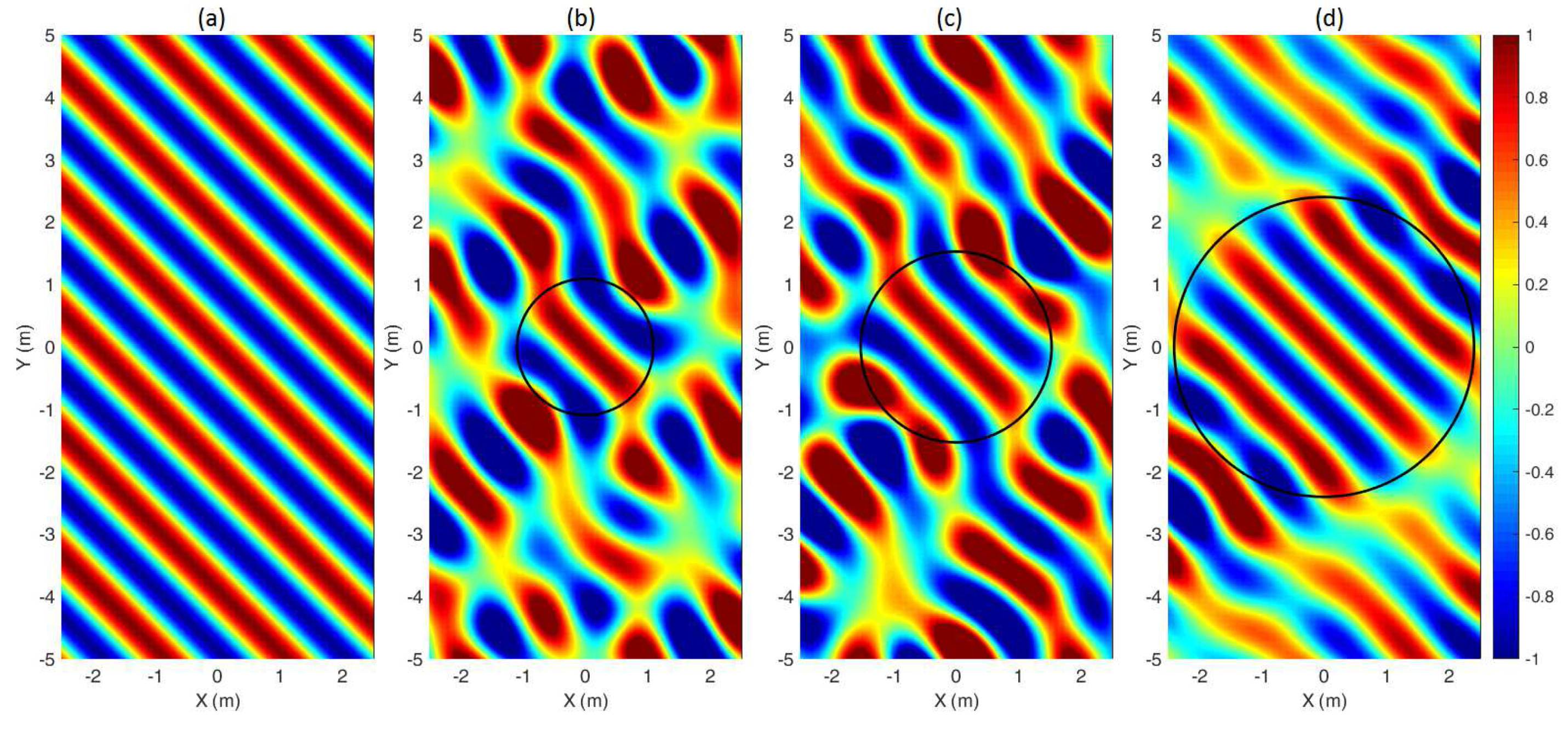
in which L is the number of plane waves, indicates the round operator, is the wavelength and R is the radius of a sphere within which the reconstruction is accurate. Numerical simulations have been performed to evaluate the effects of discretizing the plane wave expansion. Figure 2 shows the real part of the target and the reconstructed acoustic pressure (Pa) in a cross-section of the domain using 36, 64 and 144 plane waves in the expansion. The frequency of the field corresponds to 250 Hz. The black circle displayed in the figure represents the area of accurate reconstruction predicted by solving Equation (14) for R.
Figure 2 indicates that the region in which the reconstruction is accurate increases when a higher number of uniformly-distributed plane waves is considered in the expansion. Good agreement was found between the radius predicted by Equation (14) and the area where the reconstruction is correct. A preliminary analysis was performed to establish the size of the microphone array and the number of plane waves required to generate an inverse matrix whose condition number is smaller than . The condition number is defined as the ratio between the largest and the smallest singular value of the propagation matrix . It has been shown in [26] that the stability of the solution provided by the inverse method is determined by the condition number; therefore, high values of this parameter indicate that errors in the model, such as noise or non-linearity of the system, will affect the result for significantly. The criterion of a condition number smaller than was motivated due to the fact that the data come from numerical simulations, which are free from measurement noise. Although the model is still affected by numerical inaccuracies, the level of this type of noise is expected to be much lower than in the case of measured noise.
Firstly, a simple incoming plane wave of 63 Hz (, ) in free field was selected as a target. The sound field was analytically calculated in a rectangular domain of dimensions (5 m, 10 m, 3 m) and captured by four different virtual cube arrays with linear dimensions of 1.2 m, 1.6 m, 2 m and 2.4 m, respectively. The spatial resolution between microphones corresponded to 0.2 m. A frequency of 63 Hz was selected as a reference since the condition number decreases with frequency, and 63 Hz therefore provides a reasonable lower threshold. Table 1 shows the condition number of matrix for different sizes of the array and numbers of planes waves uniformly distributed over a unit sphere [25].
As expected, the condition number decreases as the size of the array increases. The reason for that may be attributed to the wavelength of the plane wave, which is approximately 5.4 m at this frequency, and a larger array captures more information of the sound field. Regarding the number of plane waves, the results suggest that increasing its number does not improve the situation, instead it increases the condition number significantly. This can be explained because at 63 Hz, there is not enough information in the sound field that is captured by the virtual microphone array; therefore, additional plane waves only make the inversion of the propagation matrix more difficult. In addition, the use of a higher number of plane waves makes the method computational expensive due to the number of convolutions that must be performed in real time. An optimal relation of 64 plane waves, a microphone array of 1.6 m in length with virtual microphone spacing of 0.2 m (729 microphone positions) was found at 63 Hz. This spatial resolution (0.2 m) yields an aliasing frequency of ≈850 Hz, which is sufficient for the range of the FE simulations. This high frequency limit is calculated based on the Nyquist theorem for sampling signals [28].
3.1. Reference Case
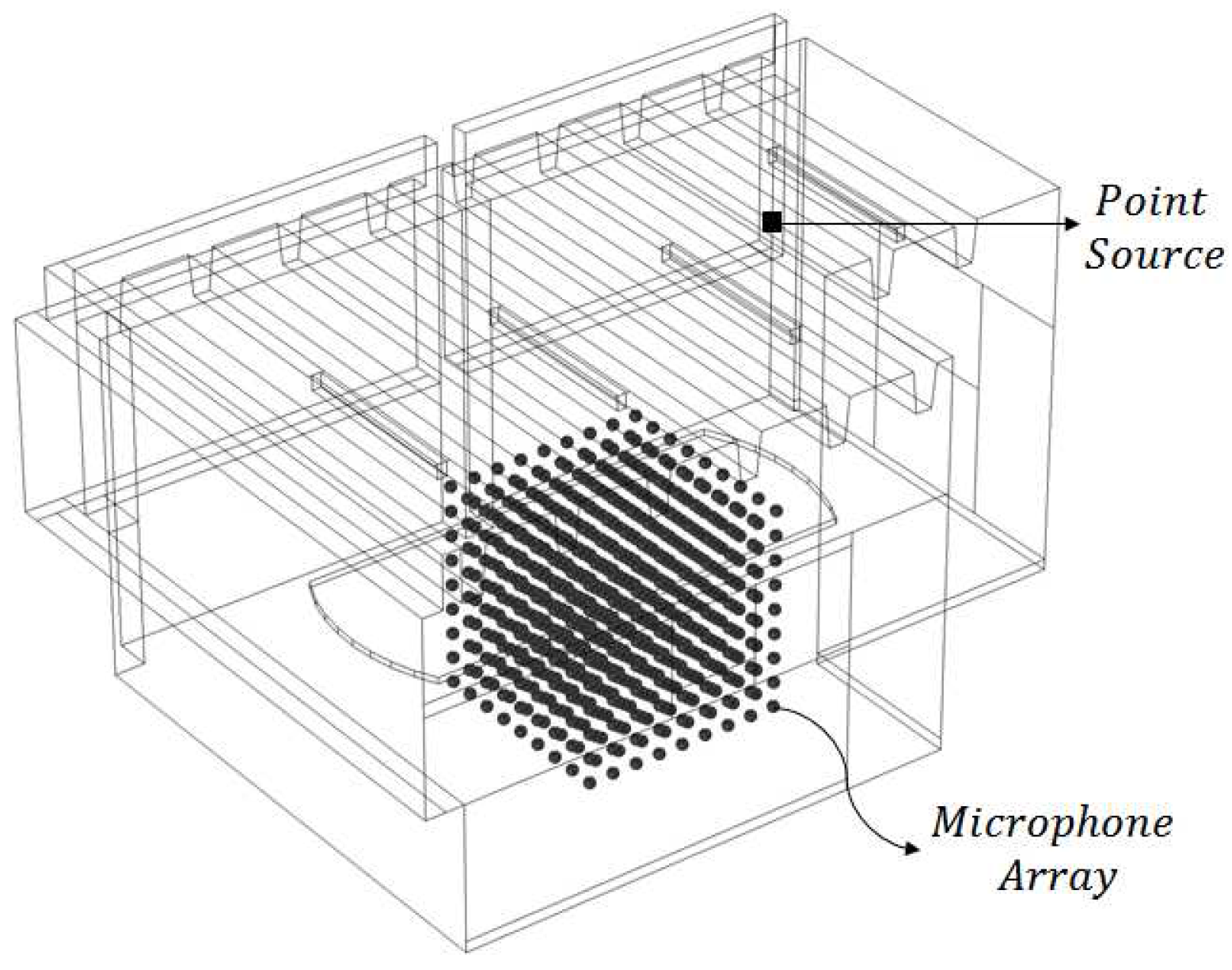
A typical meeting room (No. 4079 in Building 13 at the Highfield Campus of the University of Southampton) was selected as a reference case. It is an L-shaped room with a volume of approximately 88 m. FE simulations were conducted using the commercial package COMSOL v5.1 (COMSOL Inc., Stockholm, Sweden). The reader is referred to [21] for a detailed description of the simulation procedure, i.e., the characterization of the acoustic source, the geometric model of the enclosure, the boundary conditions and the measurements carried out to validate the predictions. Figure 3 shows a model of the enclosure identifying the location of the virtual microphone array.
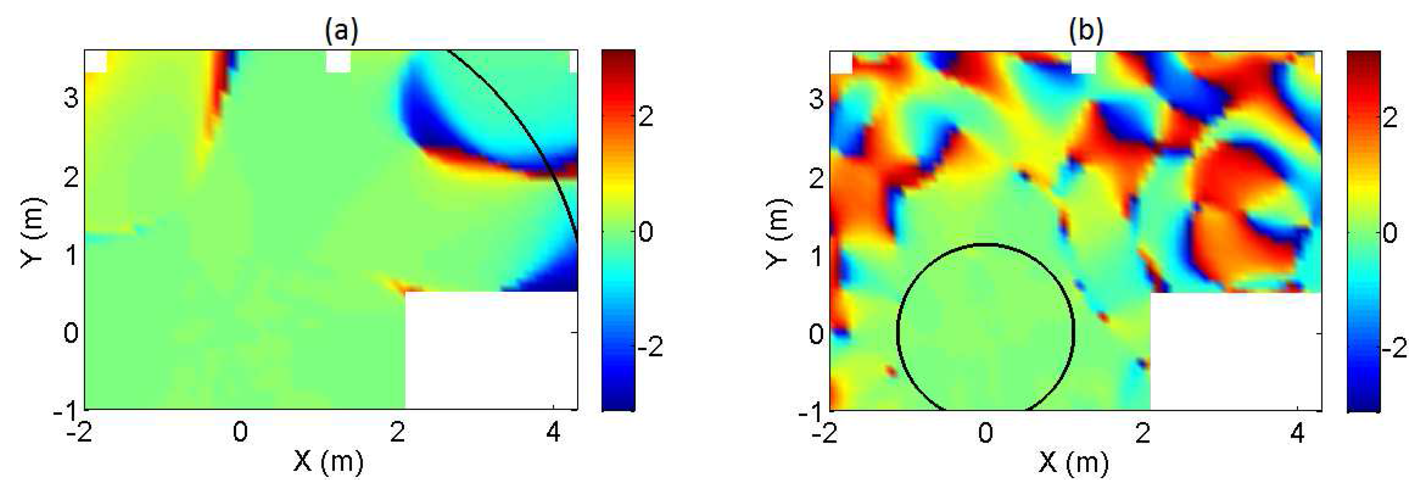
Two types of figures are presented to assess the performance of the inverse method. The first shows a comparison between the real parts of the target (numerical) and reconstructed acoustic pressures (Pa) over a cross-section of the domain (1.6 m). The second type of figure plots the absolute and phase components of the error between the target and reconstructed pressure fields, defined as:
amplitude error:
phase error:
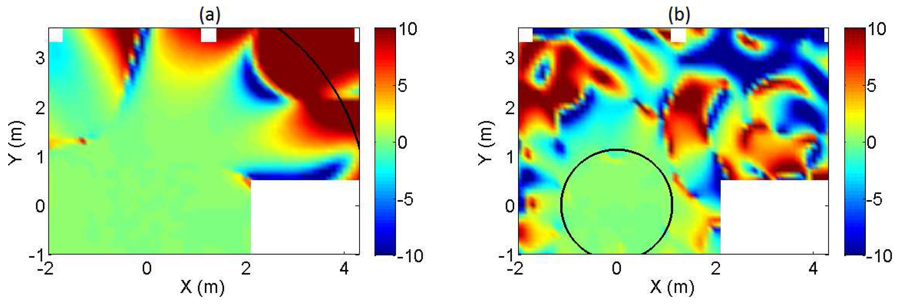
where is the reconstructed pressure, is the target pressure, indicates the complex conjugate operator and ∠ represents the phase of a complex number. The amplitude error gives insight about whether the reconstructed acoustic field is louder or quieter compared to the target one. The phase error indicates the phase differences between the reconstructed and target acoustic fields. Figure 4 and Figure 5 show the synthesized acoustic pressure at two frequencies (63 Hz and 250 Hz). The dotted black square represents the position of the microphone array.
Figure 4 and Figure 5 indicate that the inverse method is able to predict quite well a plane wave expansion whose complex amplitudes synthesize the computed sound field even in small rooms and at low frequencies where the plane wave propagation assumption is not completely satisfied. As expected, the reconstruction is accurate around the virtual microphone array. The corresponding acoustic errors are presented in Figure 6 and Figure 7, respectively.
These indicate that the area of accurate reconstruction depends on the frequency of the acoustic field, being more extensive at low frequencies. In terms of defining a radius within which the reconstruction is accurate, the acoustic errors show good agreement with Equation (14), represented by the circular arc in Figure 6 and Figure 7, only for the higher frequency of 250 Hz. At the lower frequency, 63 Hz, the area is overestimated. This relates to the presence of the walls. At the lower frequency, the homogeneous Helmholtz equation is not satisfied within the radius predicted by Equation (14) since the walls of the room intrude into this region acting as reflective boundaries and playing a role similar to acoustic sources.
3.1.1. Regularization in the Formulation of the Inverse Problem
A well-established technique to improve the stability of the solutions of inverse methods is the use of regularization in the inversion of the propagation matrix [29,30]. Tikhonov regularization is used for this purpose. It is based on the concept of changing the cost function by the inclusion of an additional term [26], that is:
where is the regularization parameter. The minimization of the cost function of Equation (17) is given by [26]:
Equation (17) indicates that the minimization of the cost function takes into account the sum of the squared errors between the reconstructed and target acoustic pressure and, in addition, the sum of the squared norm of plane wave amplitude vector. Figure 8, Figure 9, Figure 10 and Figure 11 show the results obtained for the reference problem when Tikhonov regularization is applied. The value of , which is given in each case, was calculated as:
in which is the spectral norm (the largest singular value) of the propagation matrix and is an arbitrary constant whose value is selected between and .
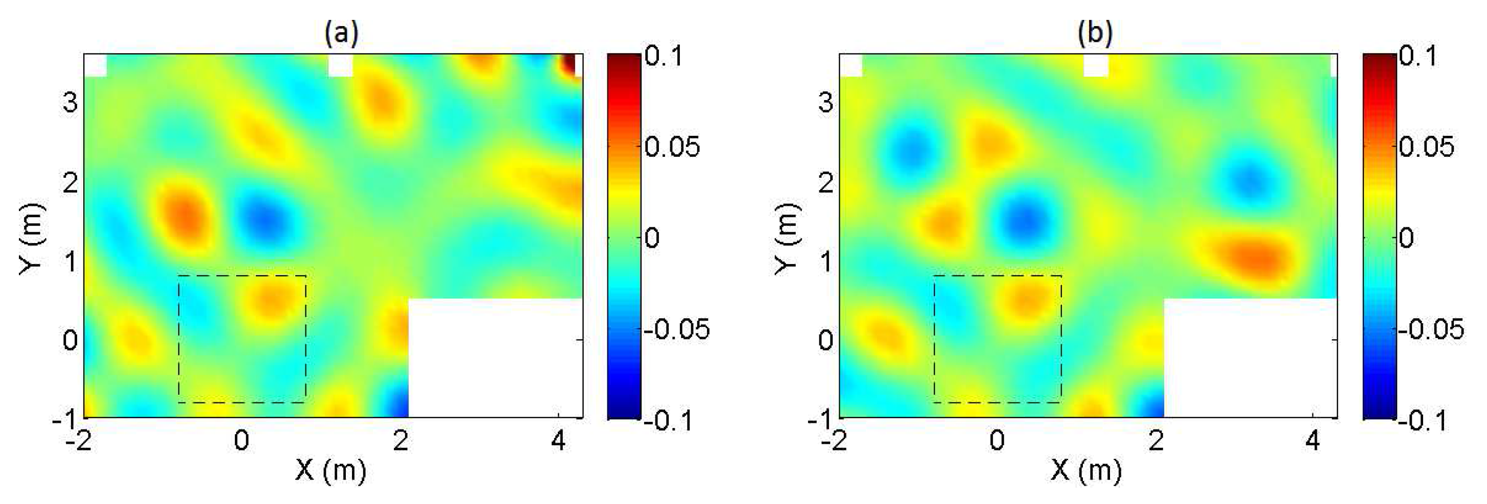
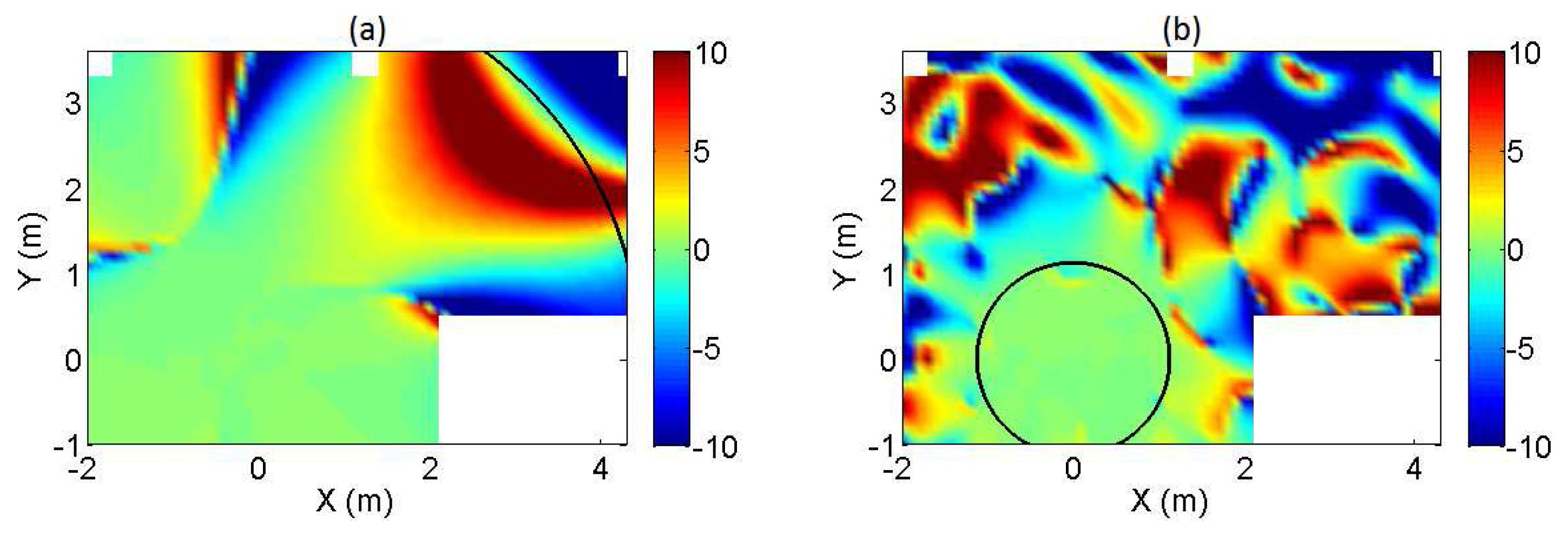
Figure 8, Figure 9, Figure 10 and Figure 11 indicate that the implementation of regularization reduces the area of accurate reconstruction at 63 Hz compared to the non-regularized case. In contrast, regularization does not have a significant effect in the sound field reconstruction at 250 Hz. This can be explained because the condition number at this frequency is low (45.9), and regularization therefore has little effect on the inversion of the matrix . Nevertheless, according to Figure 6 and Figure 10, the amplitude of the acoustic field tends to be quieter for the regularized case at 63 Hz. This particular result is convenient for an interactive auralization system because the translation operator can lead to a zone with high acoustic pressure if no regularization is applied, which affects the stability and robustness of the implementation.
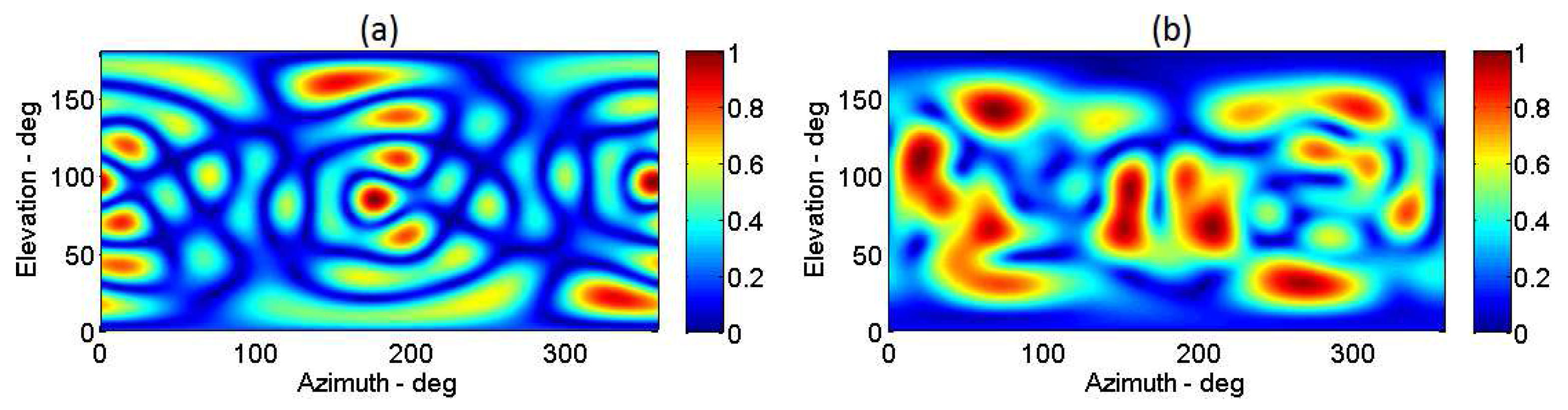
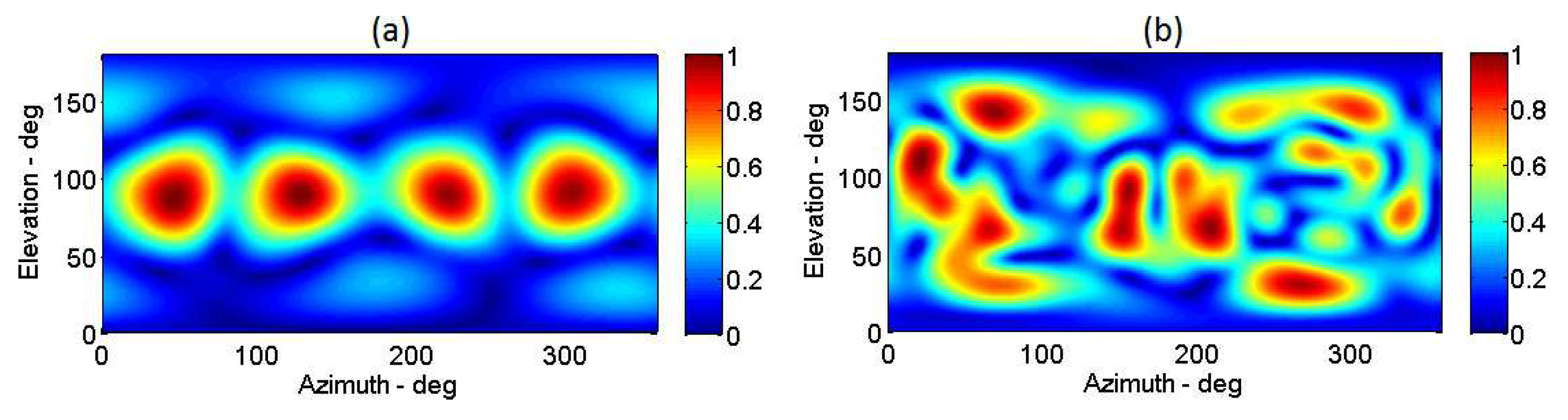
An additional analysis of the energy distribution of the plane wave density was conducted to evaluate the effects of regularization in the formulation of the inverse problem. Figure 12 and Figure 13 show an interpolated distribution of the complex amplitude of the plane waves. This is plotted in two dimensions by unwrapping the unit sphere onto a 2D plane whose axes represent the elevation and azimuth angle in degrees. The total energy of the plane wave expansion is calculated from the expression:
in which is the complex amplitude of the l-th plane wave. This value is noted in the figure captions.
These figures indicate that regularization has an important effect on the spatial distribution of the energy of the plane wave density at 63 Hz. For this frequency, a more concentrated directional representation was found when regularization is implemented. Figure 14 shows the energy of each plane wave component for the regularized and non-regularized solution. A significant reduction in the energy of the plane waves is evident in the regularized case (up to four orders of magnitude). This result suggest that the use of regularization leads to a more efficient solution in terms of the energy used to reconstruct the acoustic field.
4. Real-Time Implementation of an Auralization System
An interactive auralization system based on the plane wave expansion was developed. The system allows for real-time acoustic rendering of enclosures by using synthesized directional impulse responses calculated in advance. Due to the pre-computation of the PWE, the proposed auralization system enables interactive features such as translation and rotation of the listener within the enclosure. However, changes in the boundary conditions or modifications of the acoustic source in terms of its directivity and spatial location are not included at this stage without recalculating the PWE. The maximum frequency simulated was 447 Hz, which is sufficient to auralize the modal behaviour of the enclosure. The time required to recalculate the PWE depends on the volume of the enclosure and the maximum frequency computed in the FE solution. For this reference case, the computation time is about one day using six nodes per wavelength on a standard desktop computer with 32 GB of RAM and Intel i7 processor. A high-pass filter (cut-off at 20 Hz) and a low-pass filter (cut-off 355 Hz) were applied to reduce the ripples produced by the truncation of the data. The proposed auralization system combines a real-time acoustic rendering with a graphical interface based on a video game environment.
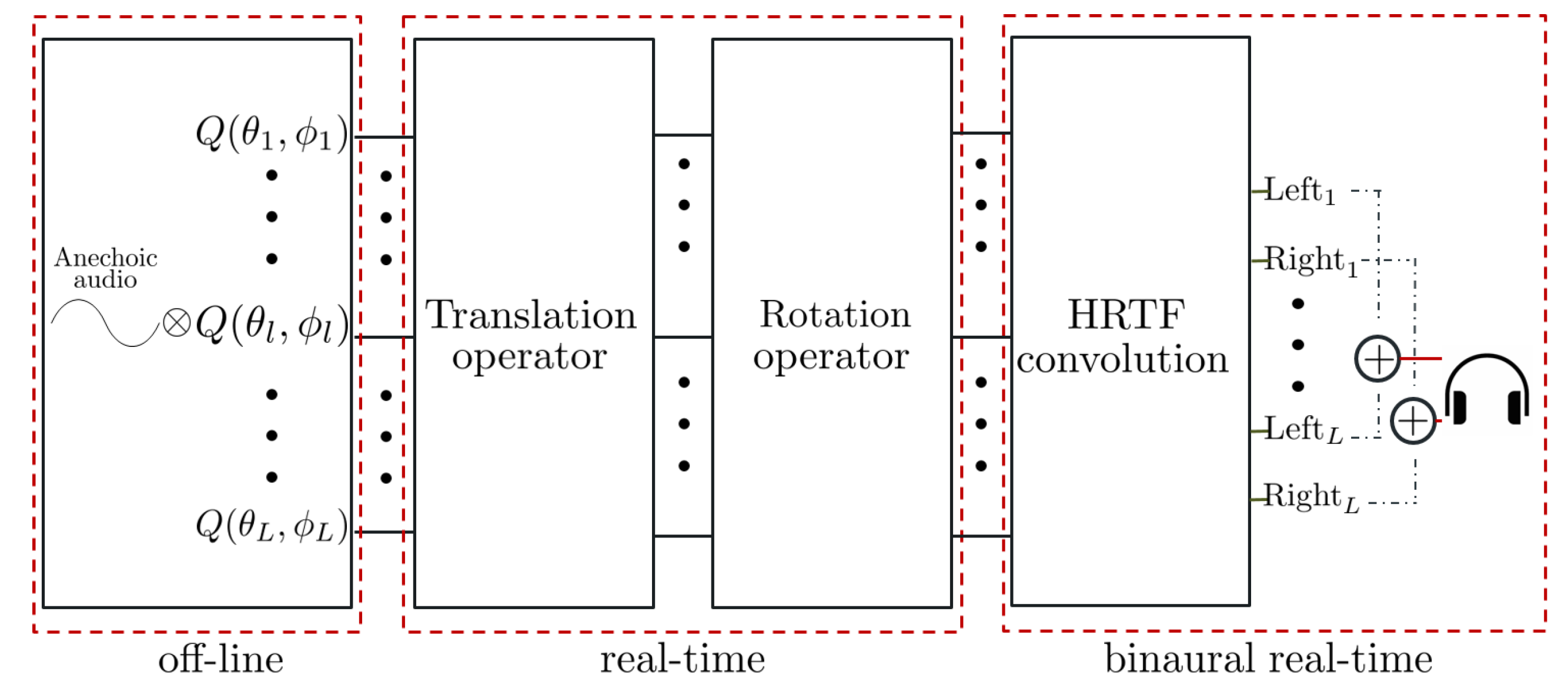
Figure 15 shows the general architecture of the signal processing chain. It is composed of four main blocks. The first block is the convolution of anechoic audio material with a plane wave expansion. The second module refers to the implementation of the translation operator in the plane wave domain. The third block corresponds to the application of a rotation operator in the spherical harmonic domain, and finally, the last stage is the sound reproduction using a headphone-based binaural system with non-individual equalization. The implementation has been made using the commercial packages Max v.7.2 and Unity v.5.0. Max is a visual programming language oriented toward audio and video processing. In contrast, Unity is a programming language dedicated to video game development. It was used in the current research to create a graphical interface for the interactive auralization.
4.1. Translation of the Acoustic Field
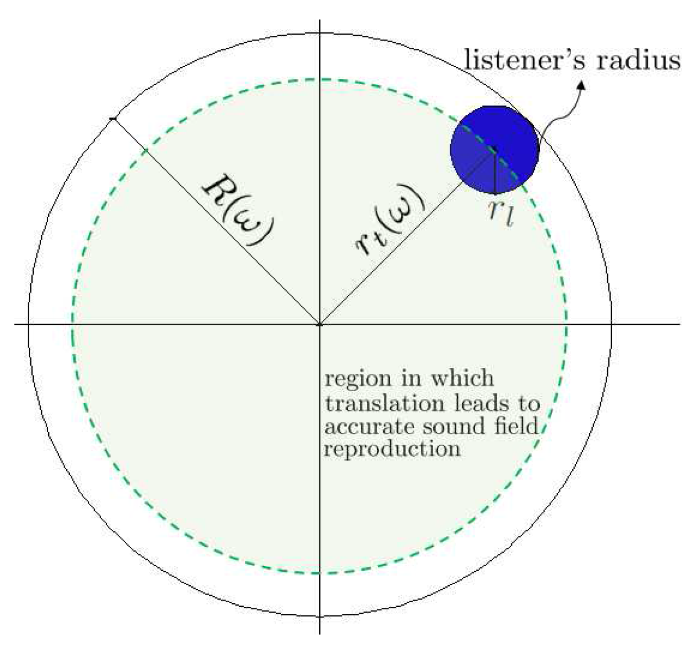
It is important to point out that the reconstructed field will be exact for the target field if an integral plane wave expansion (Equation (1)) is used for the synthesis. This outcome means that the translation operator will lead to the correct field regardless of the location where the translation is intended. However, if the plane wave expansion is approximated by a finite sum, as in Equation (8), the reconstructed field will contain errors, and the translation operator will lead to the correct field only in the area where the discretized plane wave expansion matches the target field. An indication of the amount of translation that can be applied before noticeable sound artefacts occur can be estimated from Equation (14) as:
where is the translation distance, L is the number of plane waves used for the synthesis, is the wavelength and is the radius of the listener’s head (e.g., 0.1 m) where it is desirable that the sound field is reproduced accurately. Indeed, must be taken into consideration in order to preserve the binaural cues. An example of the translation radius is given in Figure 16, in which .
4.2. Rotation of the Acoustic Field
Although sound field rotation can be generated by interpolating HRTFs, this methodology has the limitation that it is restricted to binaural reproduction only. The use of a spherical harmonic representation to rotate the acoustic field is suitable for several audio reproduction techniques, which increases the flexibility of the proposed approach. In general, the implementation of the rotation in the auralization system using a spherical harmonic transformation can be divided into three main steps: the encoding, rotation and decoding stages, respectively. The general concept can be defined as the encoding of each of the directional impulse responses into a finite number of spherical harmonic coefficients, the application of the rotation and, finally, the return to the plane wave domain again through a decoding process. Nevertheless, to reduce the computational cost required by the generation of the rotation in the acoustic field, the encoding stage is computed by using as an input the difference between the angles of the directional impulse responses and the rotation angle, rather than by multiplying the spherical harmonic coefficients by a rotation operator. Figure 17 shows the signal processing chain for the rotation operator.
One relevant consideration on the use of this approach is the number of audio files to be processed in real time (). Due to the very large amount of operations, the number of spherical harmonic coefficients was limited to the fifth order (36 coefficients) for the encoding and decoding stages. The encoding is performed using real-valued spherical harmonics [31], which are calculated from their complex pairs. As a consequence of the reduced order used for rotation, the area of accurate reconstruction is reduced following the relation . In order to preserve the translation area, the translation operator is applied before the rotation. In this case, the area reduction given by the lower spherical harmonic order does not reduce the region where the translation operator accurately reconstructs the target field. This means that the outcome of the rotation operation has only to be accurate in the radius corresponding to the listener’s head (). The truncation of the spherical harmonic series up to fifth order is sufficient to cover the listener’s radius for the frequency range considered.
4.3. Graphical Interfaces
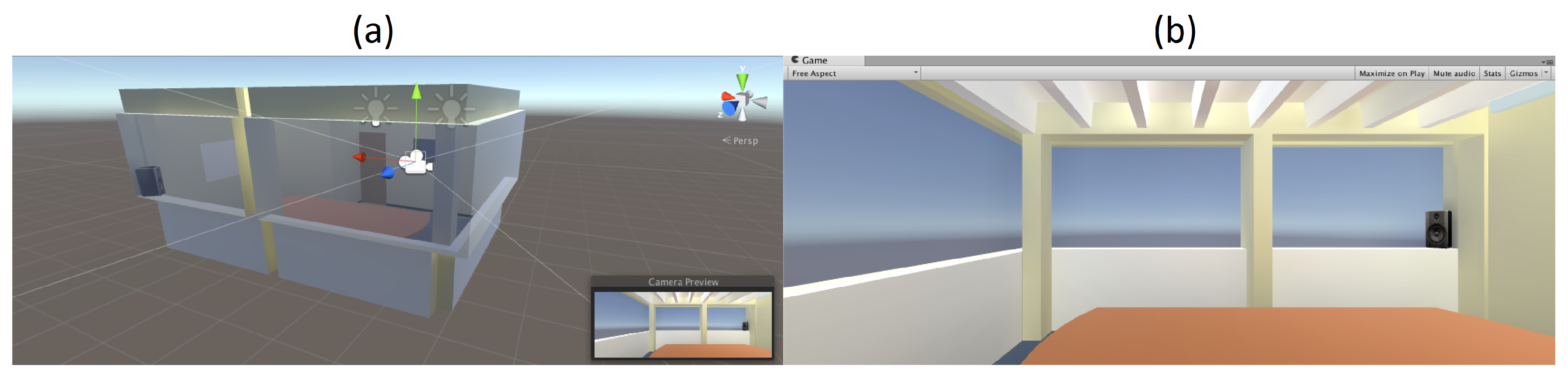
A virtual environment was created in Unity to generate a platform where the listener can move using a first-person avatar and hear the changes in the acoustic field based on its relative position with respect to the enclosure. This is achieved by sending from Unity to Max the location and orientation of the avatar. The interaction between these two software packages was achieved using the Max-Unity Interoperability Toolkit [32]. Figure 18 illustrates the model made in Unity to generate the interactive auralizations.
5. Evaluation of the Auralization System
A series of experiments to assess the accuracy of the sound field reconstruction given by the proposed method is presented. For this, the real-time implementation in Max was used to record the synthesized acoustic field at different positions of the enclosure. Two types of analysis were performed: monaural (based on omnidirectional signals) and a spatial evaluation based on first order B-format signals. The procedure consisted of recording the output signals from the real-time auralization system implemented in Max and comparing them to numerical references from the FE model.
5.1. Monaural Analysis
A comparison of the predicted omnidirectional frequency responses at different receiver positions was carried out. This was performed by rendering the sound field in real time using the auralization system developed in Max. The omnidirectional frequency responses from the auralization system were obtained by adding all of the directional impulse responses corresponding to the different L plane waves used to represent the field and recording the total output after the rotation stage. This information is compared to omnidirectional frequency responses that were synthesized individually at the receiver locations. These omnidirectional references do not use the directional information of the plane wave expansion. They correspond to the frequency response of omnidirectional receivers obtained directly from the FE solution. The use of the numerical information as a reference is due to the lack of measurements and spatial information across the enclosure to evaluate different positions.
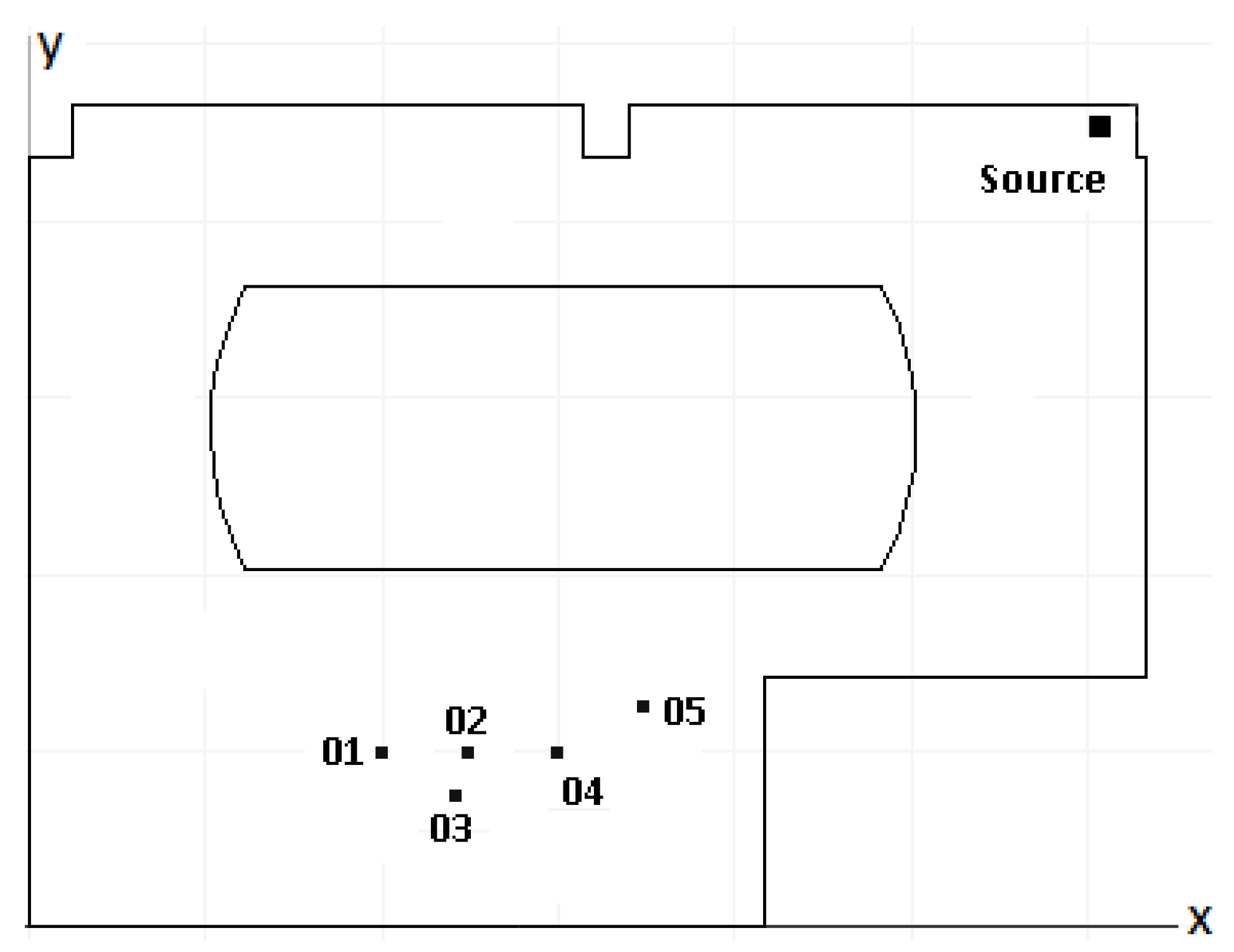
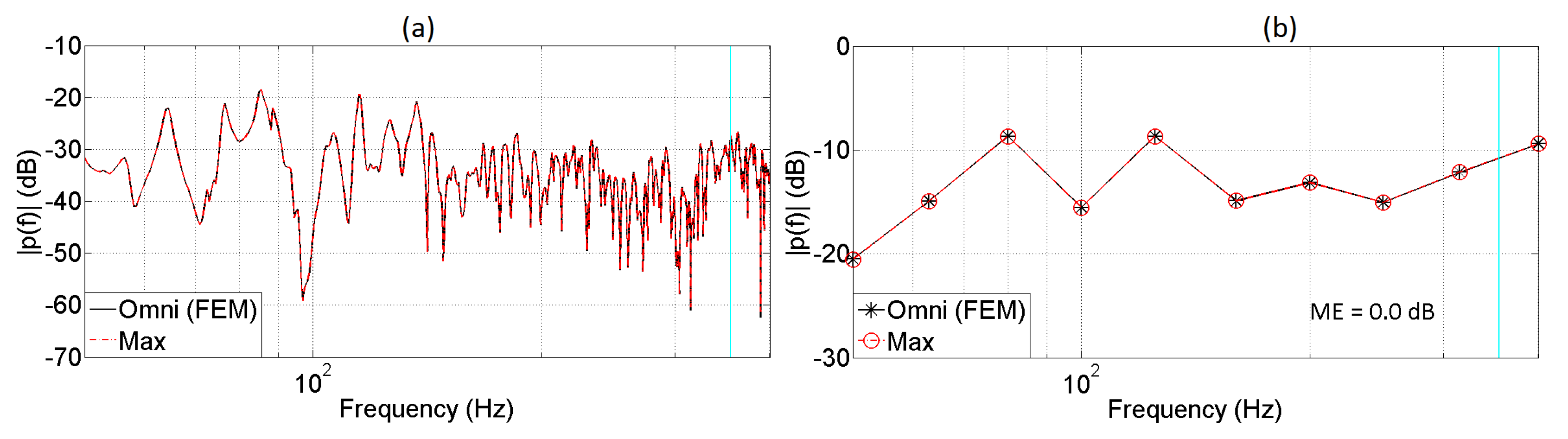
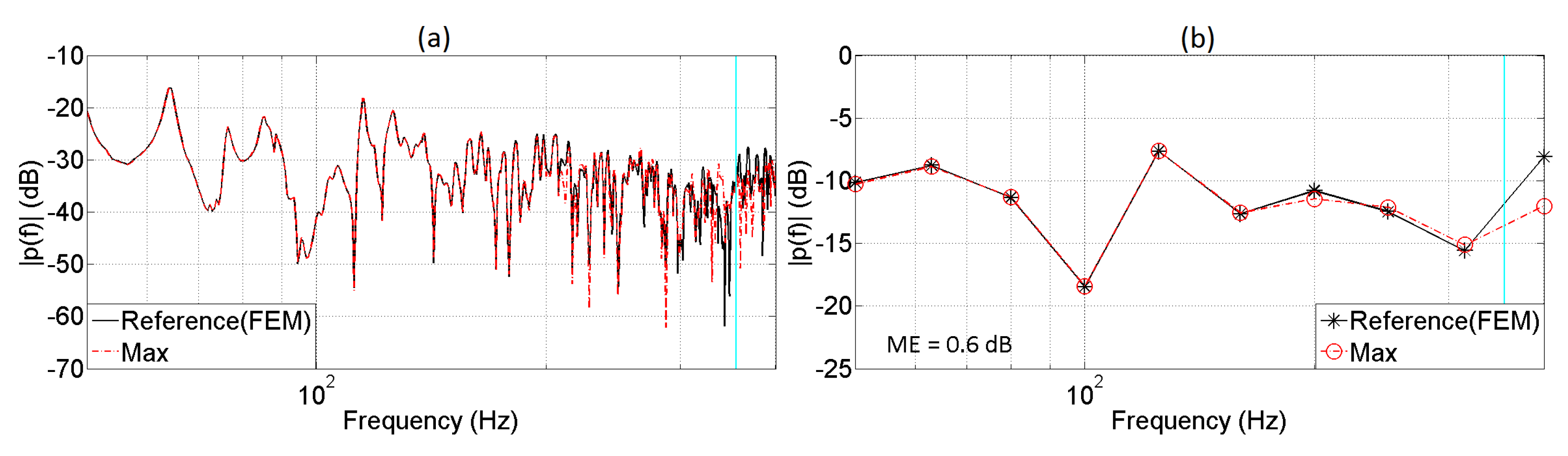
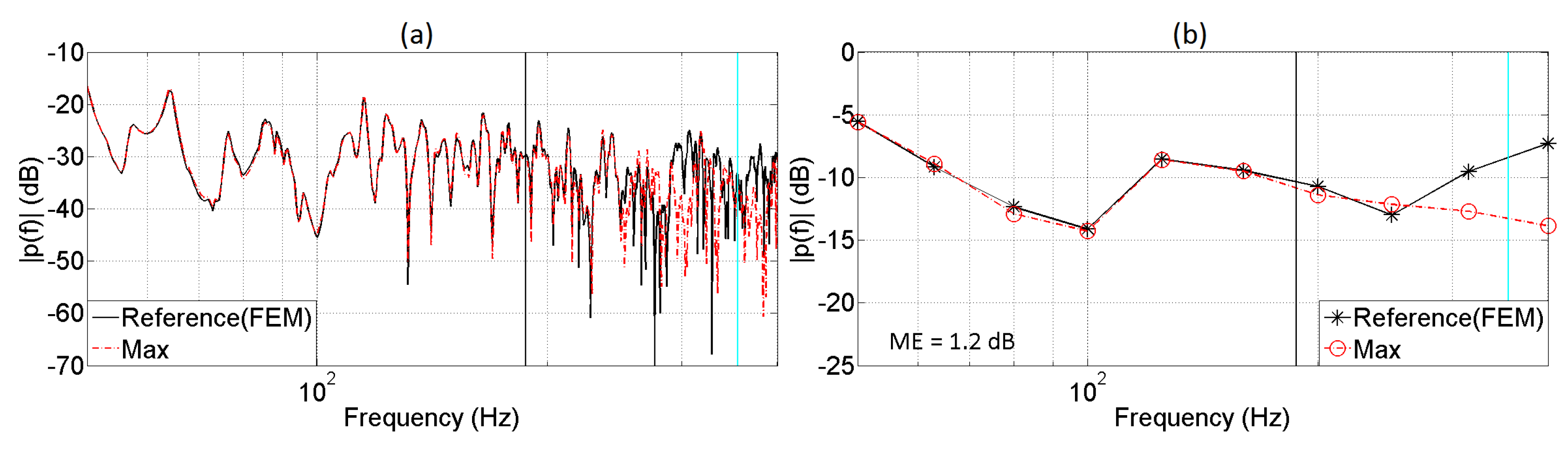
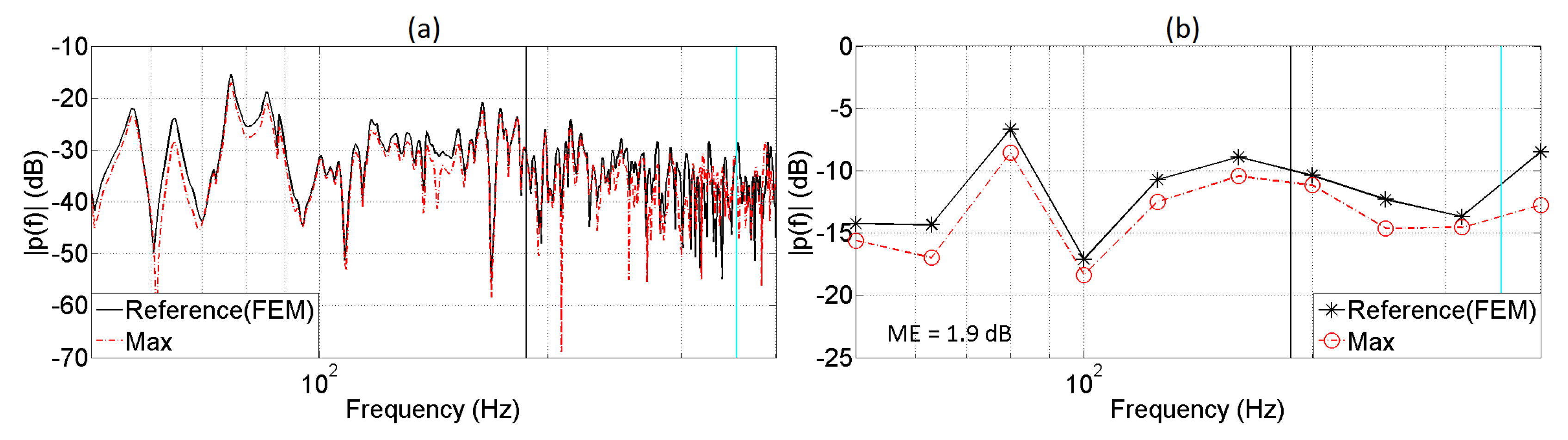
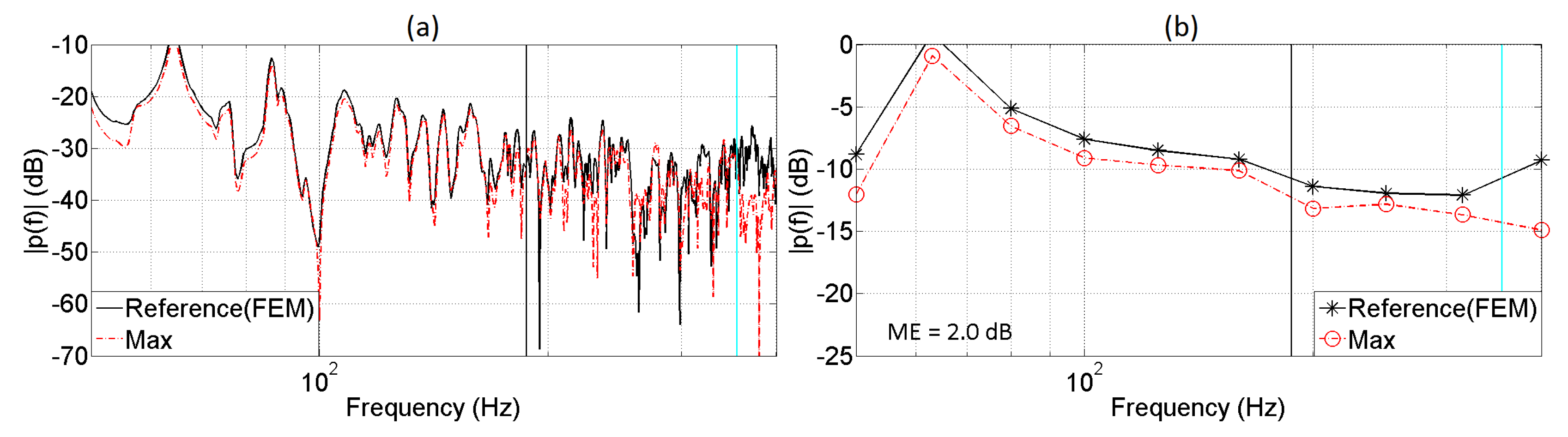
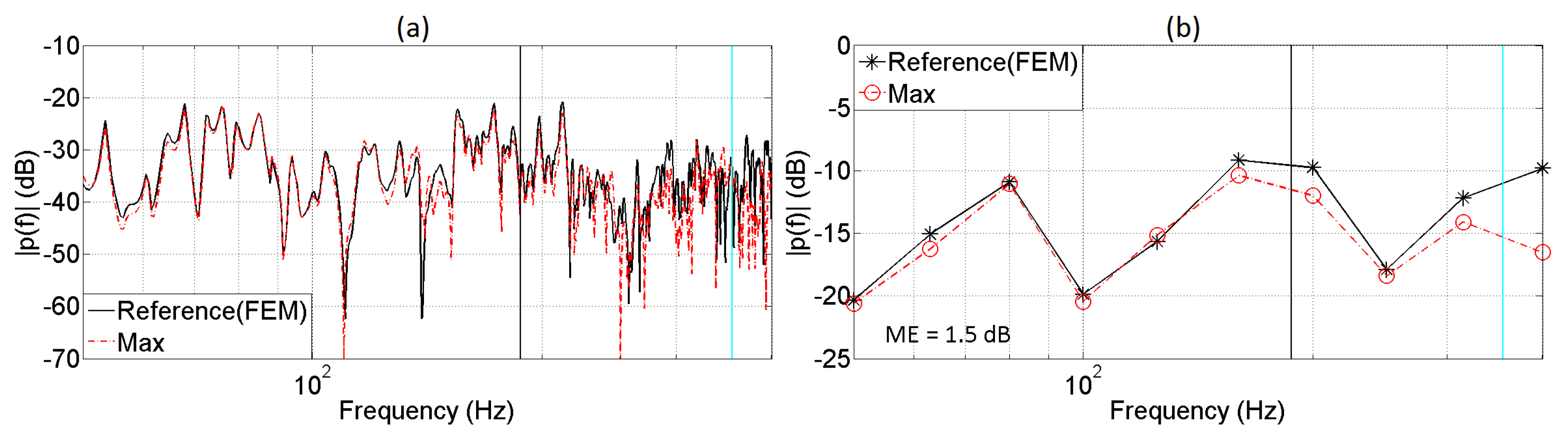
Five receivers’ positions were selected as shown in Figure 19. The central point of the expansion corresponds to Location 01. The predicted frequency responses in narrow band and in 1/3 octave band resolution for each receiver are illustrated in Figure 20, Figure 21, Figure 22, Figure 23 and Figure 24. The vertical cyan line indicates the cut-off frequency (355 Hz) of the low-pass filter, and the vertical black line indicates the maximum frequency below which the translation is expected to provide accurate results. The maximum frequency was estimated by solving Equation (14) for R. This was done taking into account the distance between the central point of the expansion and each receiver’s position. The mean error displayed in the figures was selected as a metric, and it is defined as:
in which n is the number of 1/3 octave frequency bands and and are the predicted and reference energy of the acoustic pressure in the 1/3 octave band i, respectively. This error is based on an equal contribution from all of the 1/3 octave bands, being analogous to a model in which pink noise is used as the input signal. It was created to provide insight into how dissimilar on average the reconstructed field is from the reference one. A summary of the mean errors according to the receiver location is presented in Table 2.
The results indicate that the changes in the modal response of the enclosure are correctly predicted by the translation operator. Furthermore, the figures show good accuracy in the sound field reconstruction up to the frequencies predicted by Equation (14) as long as these frequencies are below the cut-off frequency. The differences found at this frequency range may arise from three causes: the implementation of integer delays in Max, the numerical accuracy used by Max to perform mathematical operations (summing the directional impulse responses) and the application of regularization in the inverse problem, which decreases the matching between the radius of validity and the effective area where the reconstruction is accurate.
5.2. Spatial Analysis
In the previous section, the auralization system was evaluated in terms of its accuracy in reconstructing the acoustic pressure at different reference locations. Although this provides useful insight into the performance of the method, it does not give any information about the spatial characteristics of the synthesized sound field. This aspect was investigated by assessing the ability of the system to accurately reconstruct the zero and first order terms in the spherical harmonic expansion of the sound field, as described by Equation (4), often referred to as Ambisonics B-format signals. An accurate reconstruction of the zero and first order sound fields at the listening position implies an accurate reproduction of binaural localization cues at low frequencies [33]. Nevertheless, this approach is a preliminary analysis, and further investigation is required.
The B-format reference signals were estimated by the implementation of an inverse method according the formulation proposed by the authors [34]. For this, virtual microphone arrays were used to sample the FE data at the positions where the B-format signals were intended to be synthesized. The B-format signals from the auralization system were obtained by recording the output of the rotation module (see Figure 15), which is based on a spherical harmonic transformation. The zero and first order components were recorded and compared to the numerical references.
The B-format consists of four signals, which correspond to an omnidirectional (zero order) and three orthogonal dipoles (first order). They are refereed to in the Ambisonics literature as W, X, Y and Z, respectively. The analysis of the B-format signals was carried out at Receivers 2 and 5. These were chosen because they corresponded to the locations where the best and worst agreement was found in terms of the mean errors for the monaural evaluation. The frequency responses in the narrow band and in the 1/3 octave band resolution of the reference and synthesized B-format signals are illustrated in Figure 25, Figure 26, Figure 27, Figure 28, Figure 29, Figure 30, Figure 31 and Figure 32. A summary of the mean errors according to the B-format component is presented in Table 3.
A comparison of the mean errors indicates that the field at Receiver 2 has smaller errors values than at Receiver 5. This is expected as the distance to the central point of the expansion of Receiver 2 is smaller. Regarding the B-format signals, the outcomes show that the reconstruction is more accurately performed for the W signals. In this case, a very good agreement between the frequency response synthesized by the auralization system and the reference signal was found up to the frequency established by Equation (14). For the remaining coefficients, the match is not as good as the zero order, but with good agreement in terms of the envelope of the frequency response.
6. Conclusions
A framework for the generation of an interactive auralization of an enclosure based on a plane wave expansion has been presented. This acoustic representation not only allows for interactive features, such as the translation and rotation of sound fields, but is also compatible with several sound reproduction techniques, such as binaural rendering, Ambisonics, WFS and VBAP. The directional impulse responses corresponding to this plane wave representation were predicted by means of the finite element method.
An analysis of the reconstruction of the sound field in terms of monaural and B-format signals indicates that the interactive auralization system based on a plane wave representation is able to synthesize the acoustic field at low frequencies correctly, making it suitable for the auralization of enclosures, whose sound field is characterized by a modal behaviour.
The suitability of inverse methods to estimate the amplitude of a set of plane waves that reconstruct a target field has been proven. This technique is useful to extract directional information from data obtained from FE simulations. However, the discretization of the integral representation into a finite number of plane waves limits the spatial accuracy of the sound field reconstruction. The extent of the region in which the synthesis is accurate depends on the number of plane waves and the frequency of the field.
The use of Tikhonov regularization has three main effects on the sound field representation. The first is that the energy of the plane wave density used for the synthesis of the sound fields is considerably lower than for the non-regularized solution. The second consequence is that the energy distribution of the plane wave density is much more directionally concentrated. The last effect is a reduction of the area where the sound field reconstruction is accurate compared to the non-regularized solution. Nevertheless, the implementation of regularization is convenient for an interactive auralization system because the translation operator can generate zones with high acoustic pressure if no regularization is applied.
Future work will include the combination of finite element and geometrical acoustic results to extend the method outlined here to middle and high frequencies.
The code developed for the interactive system can be download from “https://drive.google.com/file/d/0BwuuNpQpY5UKZ2htSW9JbXN5OVU/view?usp=sharing”.
Author Contributions
The current paper is the result of the research conducted by Diego Mauricio Murillo Gómez for the degree of doctor of philosophy at the Institute of Sound and Vibration Research, University of Southampton. Filippo Maria Fazi and Jeremy Astley were the supervisors; their contributions correspond to the advice, support and review at all stages of the research.
Conflicts of Interest
The authors declare no conflict of interest.
Abbreviations
The following abbreviations are used in this manuscript:
| GA | Geometrical Acoustics |
| FEM | Finite Element Method |
| BEM | Boundary Element Method |
| FDTD | Finite Difference Time Domain |
| GPU | Graphics Processor Unit |
| PWE | Plane Wave Expansion |
| WFS | Wave Field Synthesis |
| VBAP | Vector-Based Amplitude Panning |
References
- Vorländer, M. Auralization, 1st ed.; Springer: Berlin, Germany, 2010. [Google Scholar]
- Savioja, L.; Huopaniemi, T.; Lokki, T.; Vaananen, R. Creating Interactive Virtual Acoustic Environments. J. Audio Eng. Soc. 1999, 47, 675–705. [Google Scholar]
- Funkhouser, T.; Tsingos, N.; Carlbom, I.; Elko, G.; Sondhi, M.; West, J.; Pingali, G.; Min, P.; Ngan, A. A beam tracing method for interactive architectural acoustics. J. Acoust. Soc. Am. 2004, 115, 739–756. [Google Scholar] [CrossRef] [PubMed]
- Noisternig, M.; Katz, B.; Siltanen, S.; Savioja, L. Framework for Real-Time Auralization in Architectural Acoustics. Acta Acust. United Acust. 2008, 94, 1000–1015. [Google Scholar] [CrossRef]
- Chandak, A.; Lauterbach, C.; Taylor, M.; Ren, Z.; Manocha, D. AD-Frustum: Adaptive Frustum Tracing for Interactive Sound Propagation. IEEE Trans. Vis. Comput. Graph. 2008, 14, 1707–1714. [Google Scholar] [PubMed]
- Taylor, M. RESound: Interactive Sound Rendering for Dynamic. In Proceedings of the 17th International ACM Conference on Multimedia 2009, Beijing, China, 19–24 October 2009; pp. 271–280. [Google Scholar]
- Astley, J. Numerical Acoustical Modeling (Finite Element Modeling). In Handbook of Noise and Vibration Control, 1st ed.; Crocker, M., Ed.; John Wiley & Sons: Hoboken, NJ, USA, 2007; Chapter 7; pp. 101–115. [Google Scholar]
- Herrin, D.; Wu, T.; Seybert, A. Boundary Element Method. In Handbook of Noise and Vibration Control, 1st ed.; Crocker, M., Ed.; John Wiley & Sons: Hoboken, NJ, USA, 2007; Chapter 8; pp. 116–127. [Google Scholar]
- Botteldooren, D. Finite-Difference Time-Domain Simulation of Low-Frequency Room Acoustic Problems. J. Acoust. Soc. Am. 1995, 98, 3302–3308. [Google Scholar] [CrossRef]
- Mehra, R.; Raghuvanshi, N.; Antani, L.; Chandak, A.; Curtis, S.; Manocha, D. Wave-Based Sound Propagation in Large Open Scenes using an Equivalent Source Formulation. ACM Trans. Graph. 2013, 32, 19. [Google Scholar] [CrossRef]
- Mehra, R.; Antani, L.; Kim, S.; Manocha, D. Source and Listener Directivity for Interactive Wave-Based Sound Propagation. IEEE Trans. Vis. Comput. Graph. 2014, 20, 495–503. [Google Scholar] [CrossRef] [PubMed]
- Raghuvanshi, N. Interactive Physically-Based Sound Simulation. Ph.D. Thesis, University of North Carolina, Chapel Hill, NC, USA, 2010. [Google Scholar]
- Savioja, L. Real-Time 3D Finite-Difference Time-Domain Simulation of Low and Mid-Frequency Room Acoustics. In Proceedings of the 13th Conference on Digital Audio Effects, Graz, Austria, 6–10 September 2010. [Google Scholar]
- Southern, A.; Murphy, D.; Savioja, L. Spatial Encoding of Finite Difference Time Domain Acoustic Models for Auralization. IEEE Trans. Audio Speech Lang. Process. 2012, 20, 2420–2432. [Google Scholar] [CrossRef]
- Southern, A.; Wells, J.; Murphy, D. Rendering walk-through auralisations using wave-based acoustical models. In Proceedings of the 17th European Signal Processing Conference, Glasgow, UK, 24–28 August 2009; pp. 715–716. [Google Scholar]
- Sheaffer, J.; Maarten, W.; Rafaely, B. Binaural Reproduction of Finite Difference Simulation Using Spherical Array Processing. IEEE Trans. Audio Speech Lang. Process. 2015, 23, 2125–2135. [Google Scholar] [CrossRef]
- Støfringsdal, B.; Svensson, P. Conversion of Discretely Sampled Sound Field Data to Auralization Formats. J. Audio Eng. Soc. 2006, 54, 380–400. [Google Scholar]
- Menzies, D.; Al-Akaidi, M. Nearfiled binaural synthesis and ambisonics. J. Acoust. Soc. Am. 2006, 121, 1559–1563. [Google Scholar] [CrossRef]
- Winter, F.; Schultz, F.; Spors, S. Localization Properties of Data-based Binaural Synthesis including Translatory Head-Movements. In Proceedings of the Forum Acusticum, Krakow, Poland, 7–12 September 2014. [Google Scholar]
- Zotter, F. Analysis and Synthesis of Sound-Radiation with Spherical Arrays. Ph.D. Thesis, University of Music and Performing Arts, Graz, Austria, 2009. [Google Scholar]
- Murillo, D. Interactive Auralization Based on Hybrid Simulation Methods and Plane Wave Expansion. Ph.D. Thesis, Southampton University, Southampton, UK, 2016. [Google Scholar]
- Duraiswami, R.; Zotkin, D.; Li, Z.; Grassi, E.; Gumerov, N.; Davis, L. High Order Spatial Audio Capture and Its Binaural Head-Tracked Playback Over Headphones with HRTF Cues. In Proceedings of the 119th Convention of the Audio Engineering Society, New York, NY, USA, 7–10 October 2005. [Google Scholar]
- Fazi, F.; Noisternig, M.; Warusfel, O. Representation of Sound Fields for Audio Recording and Reproduction. In Proceedings of the Acoustics 2012, Nantes, France, 23–27 April 2012; pp. 1–6. [Google Scholar]
- Williams, E. Fourier Acoustics, 1st ed.; Academic Press: London, UK, 1999. [Google Scholar]
- Fliege, J. Sampled Sphere; Technical Report; University of Dortmund: Dortmund, Germany, 1999. [Google Scholar]
- Nelson, P.; Yoon, S. Estimation of Acoustic Source Strength By Inverse Methods: Part I, Conditioning of the Inverse Problem. J. Sound Vib. 2000, 233, 639–664. [Google Scholar] [CrossRef]
- Ward, D.; Abhayapala, T. Reproduction of a Plane-Wave Sound Field Using an Array of Loudspeakers. IEEE Trans. Audio Speech Lang. Process. 2001, 9, 697–707. [Google Scholar] [CrossRef]
- Herlufsen, H.; Gade, S.; Zaveri, H. Analyzers and Signal Generators. Handbook of Noise and Vibration Control, 1st ed. Crocker, M., Ed.; John Wiley & Sons: Hoboken, NJ, USA, 2007; Chapter 40. 101–115. [Google Scholar]
- Kim, Y.; Nelson, P. Optimal Regularisation for Acoustic Source Reconstruction by Inverse Methods. J. Sound Vib. 2004, 275, 463–487. [Google Scholar] [CrossRef]
- Yoon, S.; Nelson, P. Estimation of Acoustic Source Strength By Inverse Methods: Part II, Experimental Investigation of Methods for Choosing Regularization Parameters. J. Sound Vib. 2000, 233, 665–701. [Google Scholar] [CrossRef]
- Poletti, M. Unified description of Ambisonics using real and complex spherical harmonics. In Proceedings of the Ambisonics Symposium 2009, Graz, Austria, 25–27 June 2009; pp. 1–10. [Google Scholar]
- Department of Music. Virginia Tech-School of Performing Arts. 2016. Available online: http://disis.music.vt.edu/main/index.php (accessed on 25 February 2017).
- Menzies, D.; Fazi, F. A Theoretical Analysis of Sound Localisation, with Application to Amplitude Panning. In Proceedings of the 138th Convention of Audio Engineering Society, Warsaw, Poland, 7–10 May 2015; pp. 1–5. [Google Scholar]
- Murillo, D.; Fazi, F.; Astley, J. Spherical Harmonic Representation of the Sound Field in a Room Based on Finite Element Simulations. In Proceedings of the 46th Iberoamerican Congress of Acoustics 2015, Valencia, Spain, 21–23 September 2015; pp. 1007–1018. [Google Scholar]
Figure 1.
Vector is represented as in the relative coordinate system .

Figure 2.
Reconstructed acoustic field using different numbers of plane waves in the expansion. (a) target field; (b) reconstructed field ; (c) reconstructed field ; (d) reconstructed field .
Figure 2.
Reconstructed acoustic field using different numbers of plane waves in the expansion. (a) target field; (b) reconstructed field ; (c) reconstructed field ; (d) reconstructed field .

Figure 3.
Model of the reference room model.

Figure 4.
Target (a) and reconstructed (b) field of the reference room, 63 Hz.
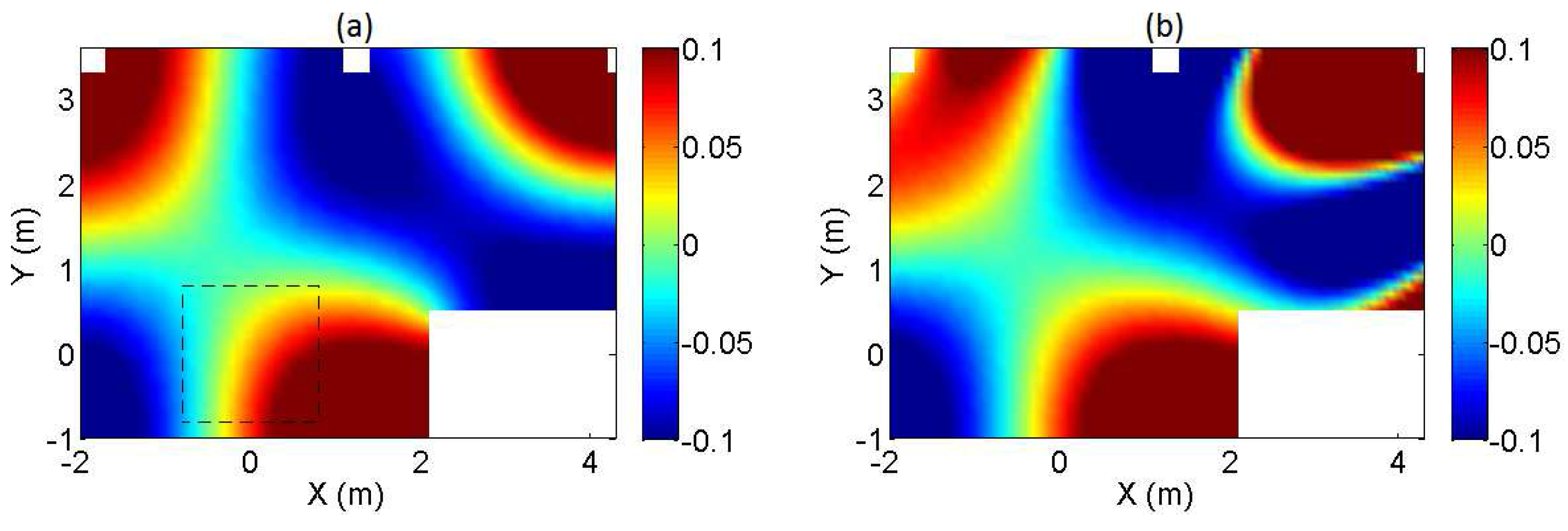
Figure 5.
Target (a) and reconstructed (b) field of the reference room, 250 Hz.
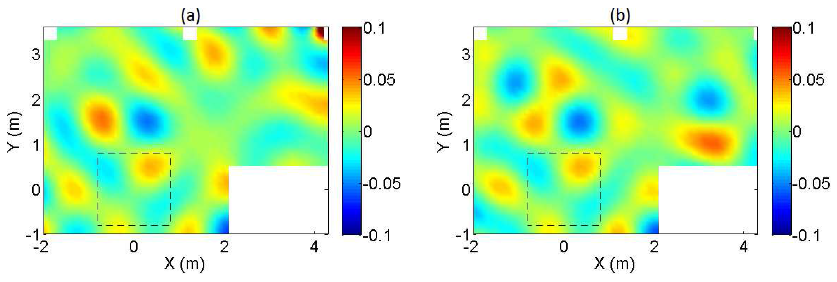
Figure 6.
Amplitude error of the reference room at 63 Hz (a) and 250 Hz (b).

Figure 7.
Phase error of the reference room at 63 Hz (a) and 250 Hz (b).

Figure 8.
Target (a) and reconstructed (b) field of the reference room, regularized .
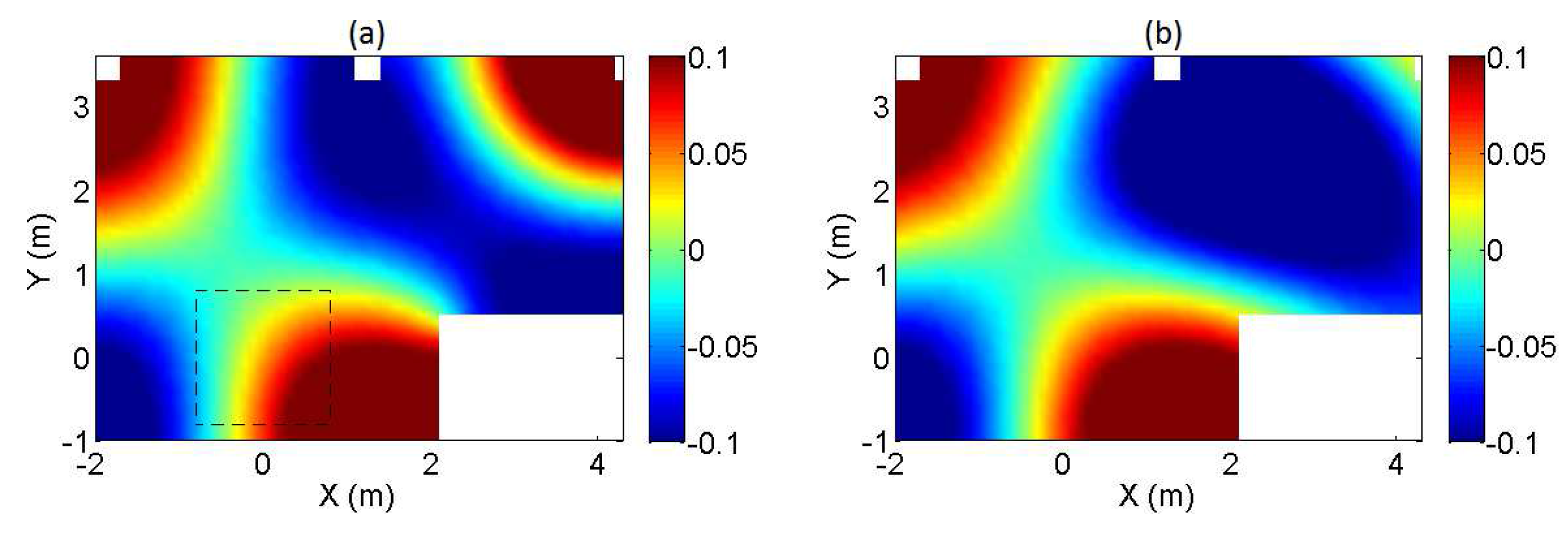
Figure 9.
Target (a) and reconstructed (b) field of the reference room, regularized .

Figure 10.
Amplitude error of the reference room at 63 Hz (a) and 250 Hz (b), regularized .

Figure 11.
Phase error of the reference room at 63 Hz (a) and 250 Hz (b), regularized .
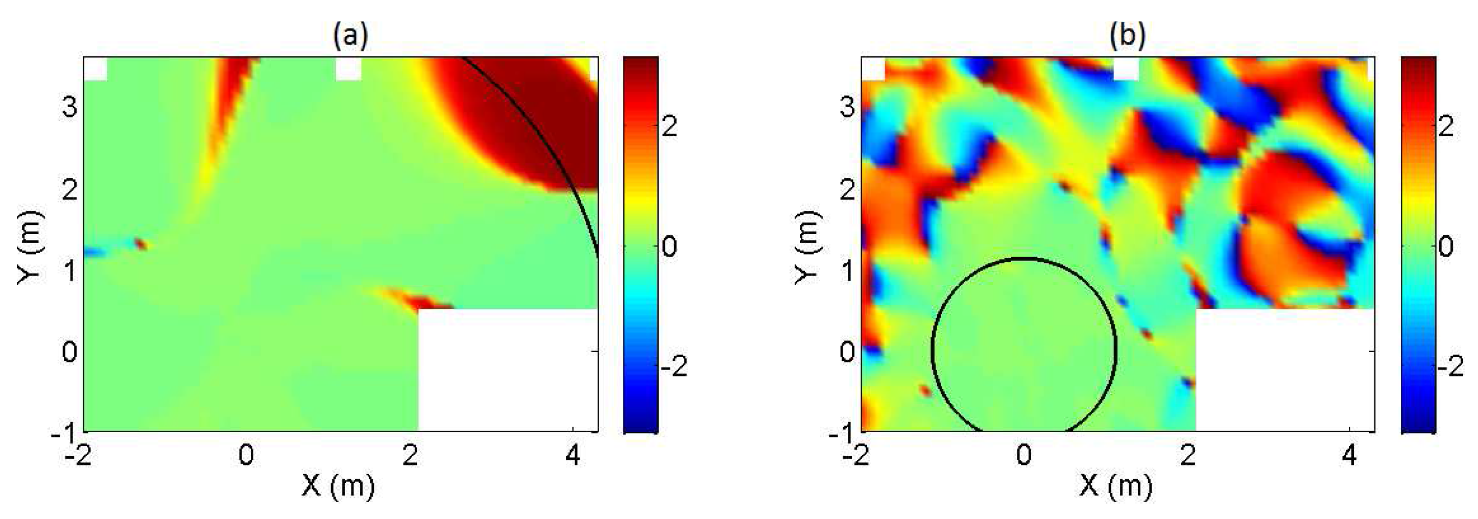
Figure 12.
Normalized amplitude PWE at 63 Hz (a) and 250 Hz (b), non-regularized, (63) = 26.11, (250) = .
Figure 12.
Normalized amplitude PWE at 63 Hz (a) and 250 Hz (b), non-regularized, (63) = 26.11, (250) = .

Figure 13.
Normalized amplitude PWE at 63 Hz (a) and 250 Hz (b), regularized , (63) = , (250) = .

Figure 14.
Comparison of the complex amplitude of the plane wave expansion.
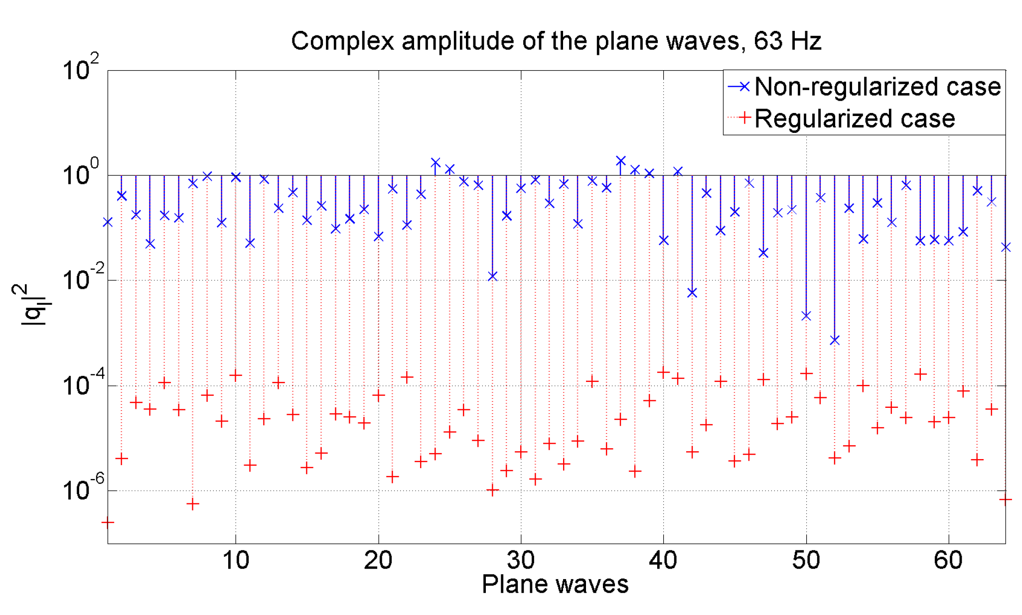
Figure 15.
General architecture for a real-time auralization based on the plane wave expansion.

Figure 16.
Region of accurate translation given by the PWE.

Figure 17.
Rotation scheme.
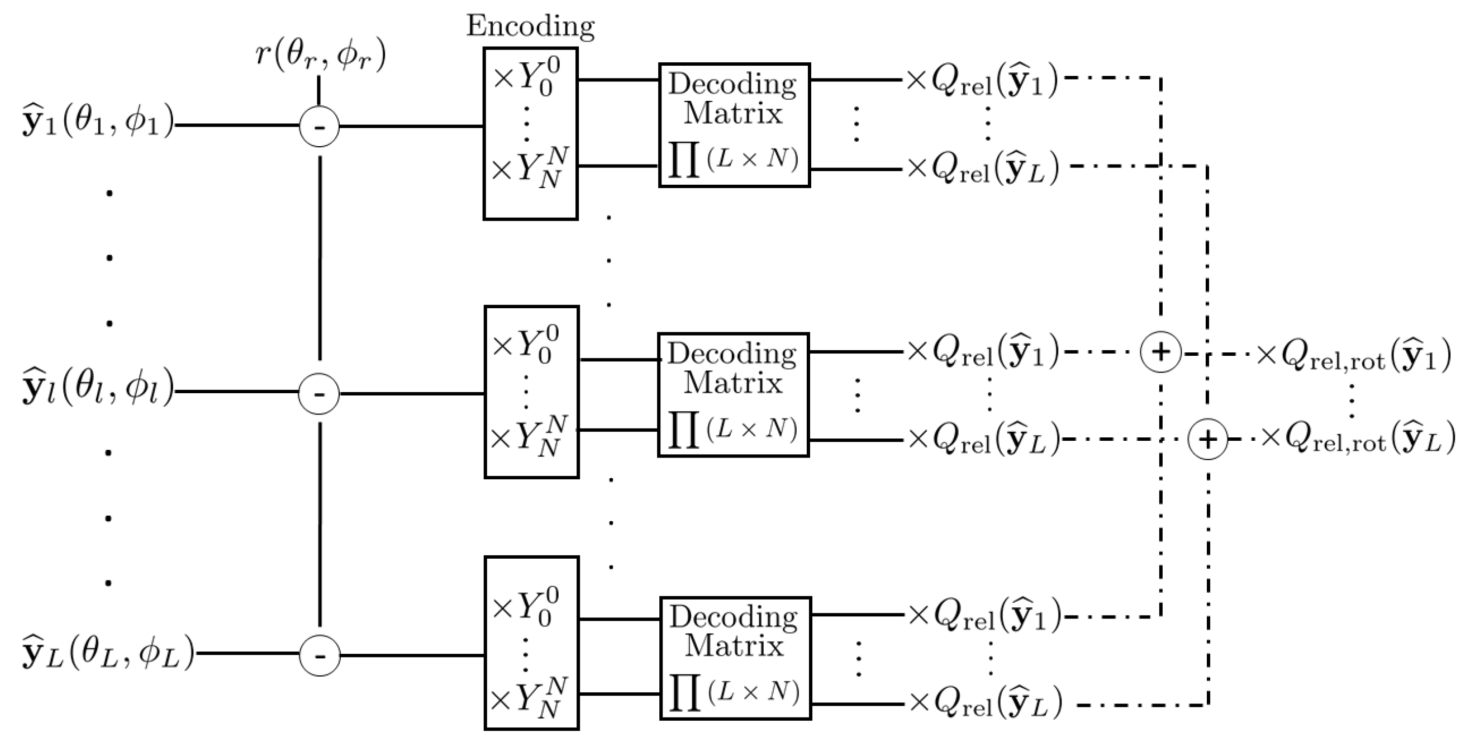
Figure 18.
Room model created in Unity. Exterior (a) and interior (b) view of enclosure.

Figure 19.
Listener positions selected to evaluate the auralization system.

Figure 20.
Comparison of full (a) and 1/3 octave band (b) frequency responses. PWE and omnidirectional room impulse response (FEM) at reference Position 1.
Figure 20.
Comparison of full (a) and 1/3 octave band (b) frequency responses. PWE and omnidirectional room impulse response (FEM) at reference Position 1.

Figure 21.
Comparison of full (a) and 1/3 octave band (b) frequency responses. Translated PWE and omnidirectional room impulse response (FEM) at translated Position 2.
Figure 21.
Comparison of full (a) and 1/3 octave band (b) frequency responses. Translated PWE and omnidirectional room impulse response (FEM) at translated Position 2.
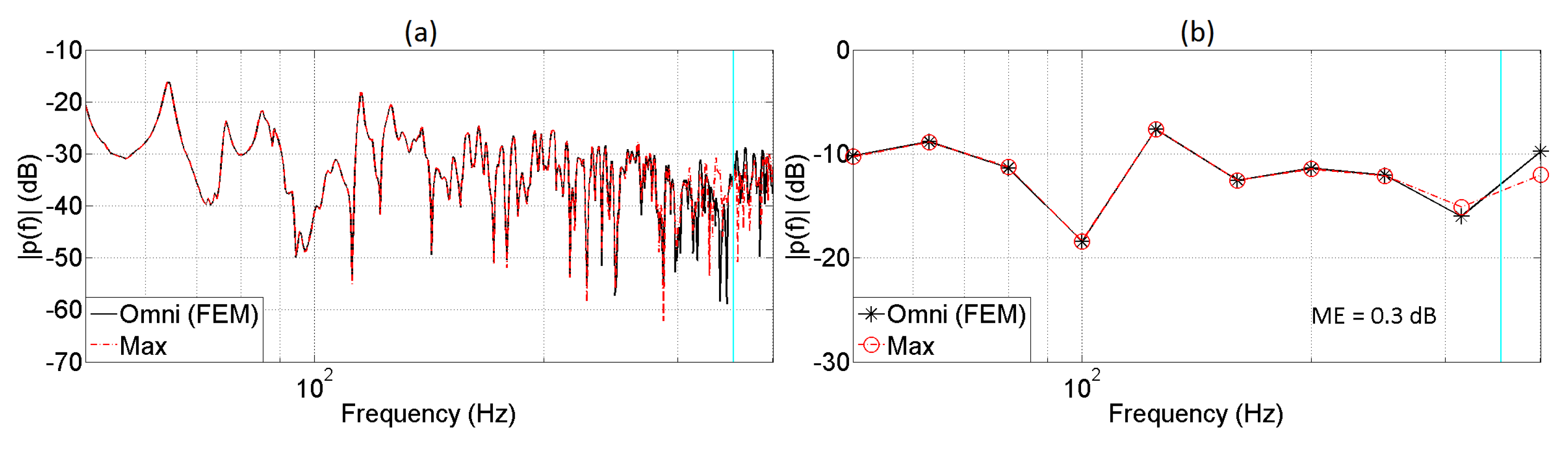
Figure 22.
Comparison of full (a) and 1/3 octave band (b) frequency responses. Translated PWE and omnidirectional room impulse response (FEM) at translated Position 3.
Figure 22.
Comparison of full (a) and 1/3 octave band (b) frequency responses. Translated PWE and omnidirectional room impulse response (FEM) at translated Position 3.
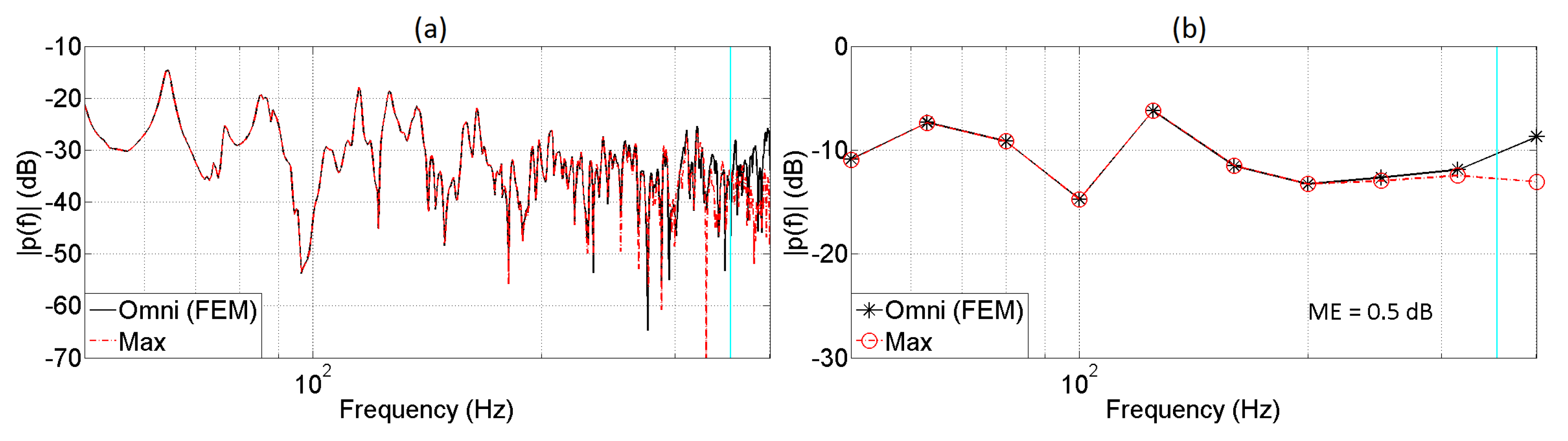
Figure 23.
Comparison of full (a) and 1/3 octave band (b) frequency responses. Translated PWE and omnidirectional room impulse response (FEM) at translated Position 4.
Figure 23.
Comparison of full (a) and 1/3 octave band (b) frequency responses. Translated PWE and omnidirectional room impulse response (FEM) at translated Position 4.
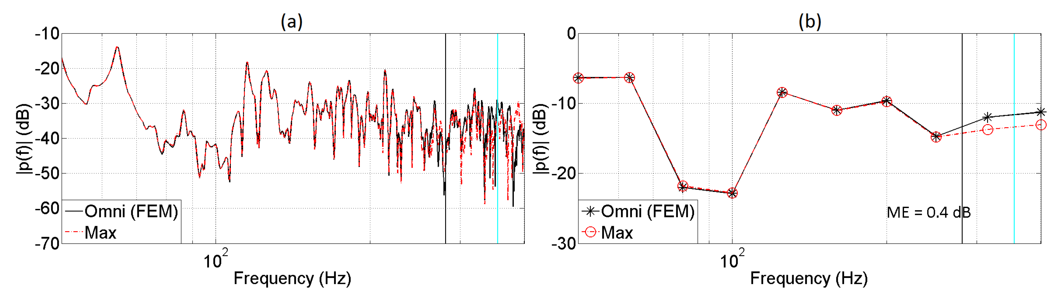
Figure 24.
Comparison of full (a) and 1/3 octave band (b) frequency responses. Translated PWE and omnidirectional room impulse response (FEM) at translated Position 5.
Figure 24.
Comparison of full (a) and 1/3 octave band (b) frequency responses. Translated PWE and omnidirectional room impulse response (FEM) at translated Position 5.
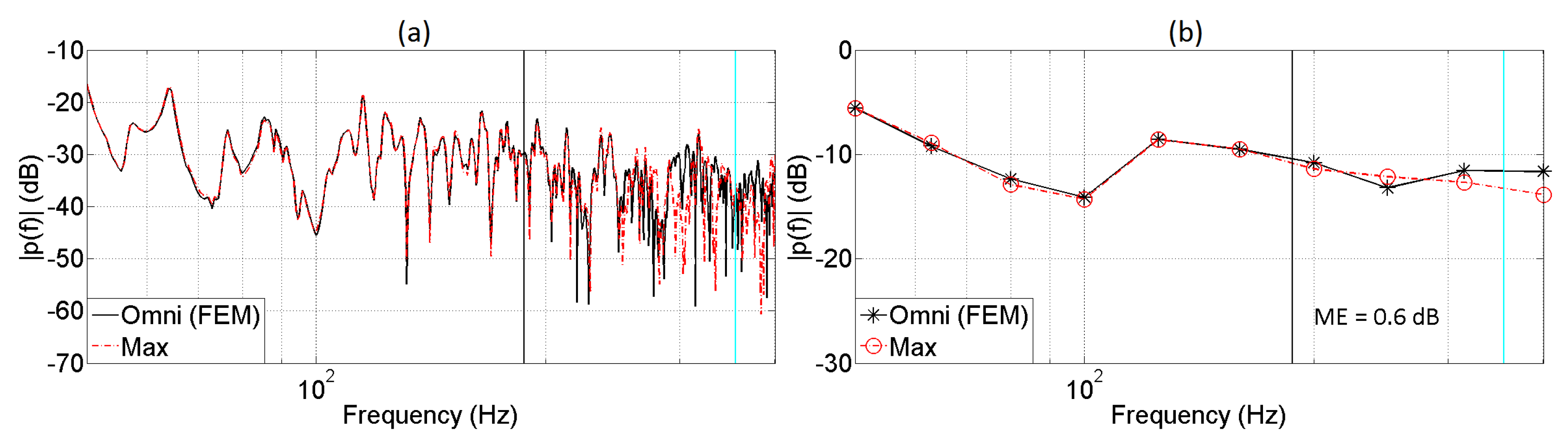
Figure 25.
Comparison of full (a) and 1/3 octave band (b) frequency responses. Translated PWE (W) and reference (W) at translated Position 2.
Figure 25.
Comparison of full (a) and 1/3 octave band (b) frequency responses. Translated PWE (W) and reference (W) at translated Position 2.

Figure 26.
Comparison of full (a) and 1/3 octave band (b) frequency responses. Translated PWE (X) and reference (X) at translated Position 2.
Figure 26.
Comparison of full (a) and 1/3 octave band (b) frequency responses. Translated PWE (X) and reference (X) at translated Position 2.
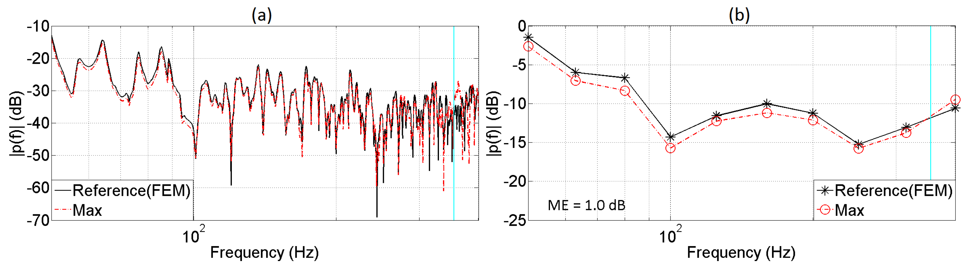
Figure 27.
Comparison of full (a) and 1/3 octave band (b) frequency responses. Translated PWE (Y) and reference (Y) at translated Position 2.
Figure 27.
Comparison of full (a) and 1/3 octave band (b) frequency responses. Translated PWE (Y) and reference (Y) at translated Position 2.
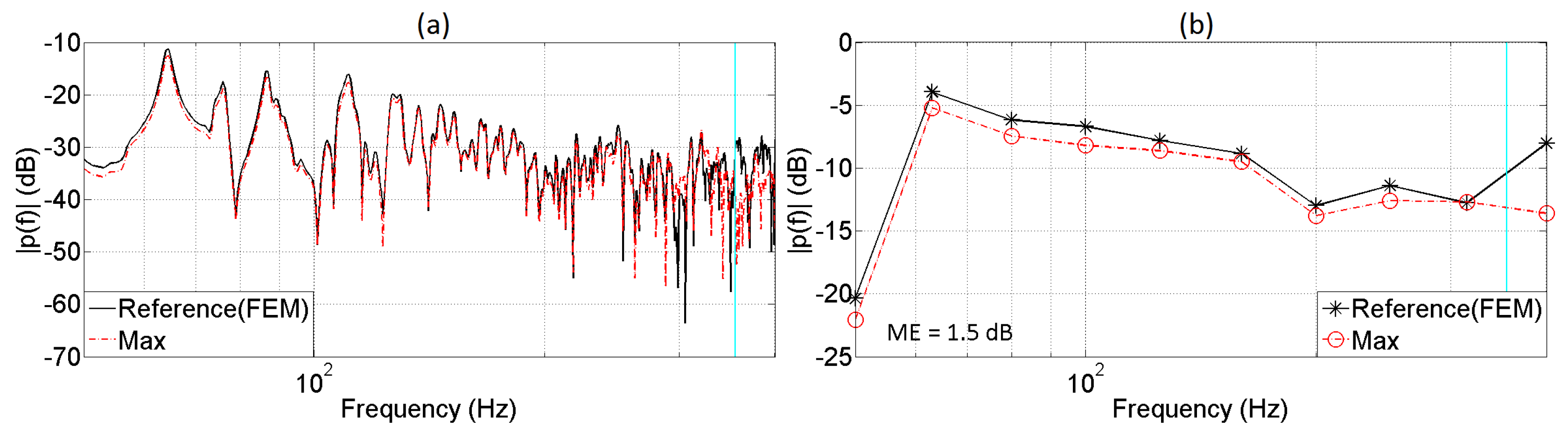
Figure 28.
Comparison of full (a) and 1/3 octave band (b) frequency responses. Translated PWE (Z) and reference (Z) at translated Position 2.
Figure 28.
Comparison of full (a) and 1/3 octave band (b) frequency responses. Translated PWE (Z) and reference (Z) at translated Position 2.
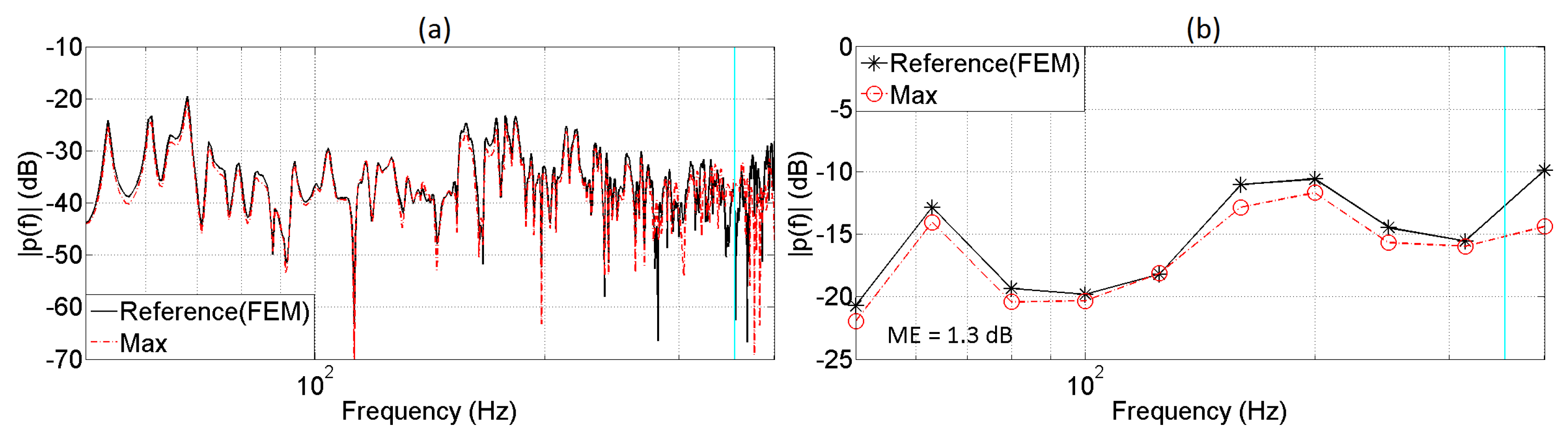
Figure 29.
Comparison of full (a) and 1/3 octave band (b) frequency responses. Translated PWE (W) and reference (W) at translated Position 5.
Figure 29.
Comparison of full (a) and 1/3 octave band (b) frequency responses. Translated PWE (W) and reference (W) at translated Position 5.

Figure 30.
Comparison of full (a) and 1/3 octave band (b) frequency responses. Translated PWE (X) and reference (X) at translated Position 5.
Figure 30.
Comparison of full (a) and 1/3 octave band (b) frequency responses. Translated PWE (X) and reference (X) at translated Position 5.

Figure 31.
Comparison of full (a) and 1/3 octave band (b) frequency responses. Translated PWE (Y) and reference (Y) at translated Position 5.
Figure 31.
Comparison of full (a) and 1/3 octave band (b) frequency responses. Translated PWE (Y) and reference (Y) at translated Position 5.

Figure 32.
Comparison of full (a) and 1/3 octave band (b) frequency responses. Translated PWE (Z) and reference (Z) at translated Position 5.
Figure 32.
Comparison of full (a) and 1/3 octave band (b) frequency responses. Translated PWE (Z) and reference (Z) at translated Position 5.


Table 1.
Condition number of the matrix as a function of the size of the microphone array and the number of plane waves.
Table 1.
Condition number of the matrix as a function of the size of the microphone array and the number of plane waves.
| Length of the Array | |||
|---|---|---|---|
| 1.2 m (343 mics) | |||
| 1.6 m (729 mics) | |||
| 2 m (1331 mics) | |||
| 2.4 m (2197 mics) |
Table 2.
Mean errors at different receiver locations. The distance to the central point of the expansion and the maximum frequency at which achieving an accurate reconstruction is expected are reported.
Table 2.
Mean errors at different receiver locations. The distance to the central point of the expansion and the maximum frequency at which achieving an accurate reconstruction is expected are reported.
| Receiver | Distance (m) | Frequency (Hz) | ME (dB) |
|---|---|---|---|
| 2 | 0.5 | ≈562 | 1.5 |
| 3 | 0.5 | ≈562 | 1.7 |
| 4 | 1 | ≈281 | 1.9 |
| 5 | 1.5 | ≈187 | 2.0 |
Table 3.
Mean errors in the B-format signals for the interactive auralization at different receiver locations.
Table 3.
Mean errors in the B-format signals for the interactive auralization at different receiver locations.
| Receiver | W (dB) | X (dB) | Y (dB) | Z (dB) | Average (dB) |
|---|---|---|---|---|---|
| 2 (0.5 m) | 0.6 | 1.0 | 1.5 | 1.3 | 1.1 |
| 5 (1.5 m) | 1.2 | 1.9 | 2.0 | 1.5 | 1.7 |
© 2017 by the authors. Licensee MDPI, Basel, Switzerland. This article is an open access article distributed under the terms and conditions of the Creative Commons Attribution (CC BY) license (http://creativecommons.org/licenses/by/4.0/).
Share and Cite
MDPI and ACS Style
Gómez, D.M.M.; Astley, J.; Fazi, F.M. Low Frequency Interactive Auralization Based on a Plane Wave Expansion. Appl. Sci. 2017, 7, 558. https://doi.org/10.3390/app7060558
AMA Style
Gómez DMM, Astley J, Fazi FM. Low Frequency Interactive Auralization Based on a Plane Wave Expansion. Applied Sciences. 2017; 7(6):558. https://doi.org/10.3390/app7060558
Chicago/Turabian StyleGómez, Diego Mauricio Murillo, Jeremy Astley, and Filippo Maria Fazi. 2017. "Low Frequency Interactive Auralization Based on a Plane Wave Expansion" Applied Sciences 7, no. 6: 558. https://doi.org/10.3390/app7060558
Note that from the first issue of 2016, this journal uses article numbers instead of page numbers. See further details here.