Prediction of Maximum Story Drift of MDOF Structures under Simulated Wind Loads Using Artificial Neural Networks

Abstract

The aim of this paper is to investigate the prediction of maximum story drift of Multi-Degree of Freedom (MDOF) structures subjected to dynamics wind load using Artificial Neural Networks (ANNs) through the combination of several structural and turbulent wind parameters. The maximum story drift of 1600 MDOF structures under 16 simulated wind conditions are computed with the purpose of generating the data set for the networks training with the Levenberg–Marquardt method. The Shinozuka and Newmark methods are used to simulate the turbulent wind and dynamic response, respectively. In order to optimize the computational time required for the dynamic analyses, an array format based on the Shinozuka method is presented to perform the parallel computing. Finally, it is observed that the already trained ANNs allow for predicting adequately the maximum story drift with a correlation close to 99%.

1. Introduction

The maximum story drift of Multi-Degree of Freedom (MDOF) structures under wind loads is an important parameter for the structural design; however, for structural engineers, the estimation of this parameter by dynamic analysis could be impractical. The dynamic analysis of structures is complex and it requires real wind speed records, which are not available in most of the cases. Several studies suggest that the use of spectral density models are adequate to simulate the velocity field of the turbulent wind [1,2,3]. Due to the complexity of obtaining synthetic wind records and the dynamic structural response, the engineers have used non-complex methods such as the equivalent static analysis, which tries to consider the dynamic effects of the turbulent wind supported by the use of the well-known dynamic amplification factor [4]. Some modifications and improvements to the equivalent static method, originally presented by Davenport [5], have been proposed by different authors [6,7]. Although these methods are not complex, they require several calculation steps in order to estimate variables such as power spectral density, background response, resonant response and others. The use of a prediction model that adequately represents a considerable amount of structures under wind loads could be useful. Nowadays, thanks to advances in computer hardware and software, Artificial Neural Networks (ANNs) have proven to be computational models capable of being applied in tasks as prediction, classification, data processing, robotic and engineering problems [8,9,10,11]. For this reason, the aim of this study is to evaluate the efficiency of ANNs as computational models for prediction of the maximum story drift of MDOF structures in terms of regional wind speeds, terrain categories and structural characteristics such as height, slenderness ratio, fundamental period, distributed mass and stiffness ratio. The Newmark method is employed to resolve the differential equation of motion. This method is frequently used in numerical evaluation of the dynamic response of structures [12,13,14]. The wind loads applied in the dynamic analyses are generated from synthetic records obtained by spectral representation with the well-known Shinozuka method [15], which has been shown to give the best results in terms of overall quality of the signal [16]. The dynamic responses of a considerable amount of MDOF structures are used to build a database about the maximum story drift related to structural characteristics and wind conditions. This database is employed to the training processes of ANNs with the Levenberg–Marquardt (LM) method, which is a standard technique for solving nonlinear least squares problems [17]. The LM method is an optimization procedure with features of stable and fast convergence [18]. The training process is applied in ANN models known as multilayer perceptrons that consist of neurons located in multiple layers and interconnected to form a network with forward propagation (Figure 1a). The multilayer perceptron approach resolve problems that are not linearly separable, which is the main limitation of the standard linear perceptron method. Hecht-Nielsen [8] proved that one hidden layer of neurons suffices to model any solution surface of practical interest. In this paper, some multilayer perceptron models with different amounts of neurons in a single hidden layer are evaluated to predict the maximum story drift of 25,600 case studies.

Figure 1b shows the internal mathematical process of each neuron. The output is given by an activation function f which depends on the sum of the inputs ${\mathrm{n}}_i{\mathrm{w}}_i$:

$$\mathrm{sum}=1{\mathrm{w}}_0+{\mathrm{n}}_1{\mathrm{w}}_1+{\mathrm{n}}_2{\mathrm{w}}_2+\dots +{\mathrm{n}}_i{\mathrm{w}}_i,$$

(1)

where ${\mathrm{n}}_i$ is the output of other neuron and ${\mathrm{w}}_i$ is the synaptic weight (Figure 1b). The sigmoid function (values between 0 and 1) is frequently used like activation function and its mathematical form is:

$$f\left(\mathrm{sum}\right)=\mathrm{n}=\frac{1}{1+e^{-\mathrm{sum}}}.$$

(2)

An important property is that its derivative can be expressed by the function itself:

$$f^{\prime }\left(\mathrm{sum}\right)=\mathrm{d}=\mathrm{n}\left(1-\mathrm{n}\right).$$

(3)

The paper is organized in the following way: Section 2 exposes the detail of the theory employed in network training, wind simulation and dynamic response. Section 3 describes the set of structural characteristics and wind conditions; then, the results of the application of theoretical framework are shown. Finally, a brief discussion of the main results is presented in Section 4.

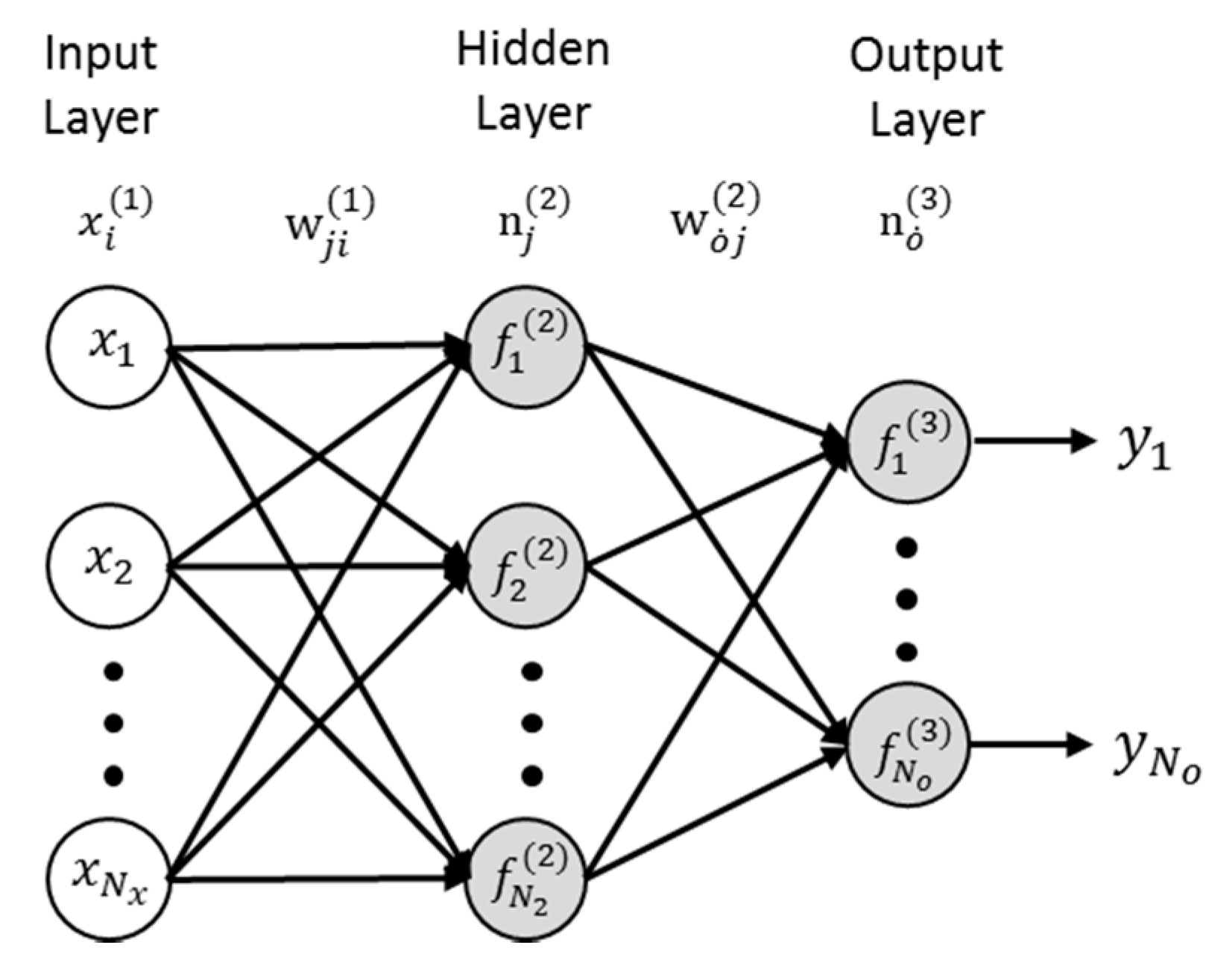
2. Theoretical Framework

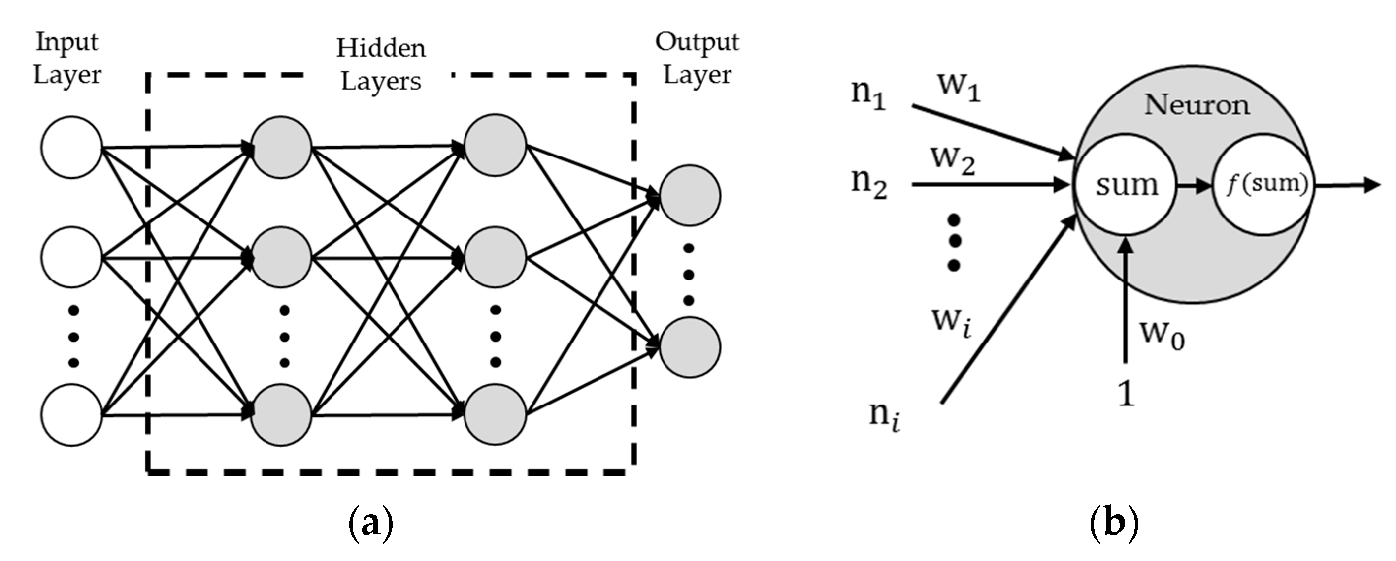
2.1. Network Training

The Sum Square Error (SSE) is a performance index and it is used in order to evaluate the training of the network:

$$E=\frac{1}{2}{{\displaystyle \sum }}_{p=1}^{N_p}{{\displaystyle \sum }}_{\dot{o}=1}^{N_o}{e}_{p\dot{o}}^2=\frac{1}{2}{{\displaystyle \sum }}_{p=1}^{N_p}{{\displaystyle \sum }}_{\dot{o}=1}^{N_o}{\left(t_{p\dot{o}}-y_{p\dot{o}}\right)}^2,$$

(4)

where $N_p$ is the number of patterns; $N_o$ is the number of outputs; $e_{p\dot{o}}$ is the error value for the pattern $p$ at the output $\dot{o}$; $t_{p\dot{o}}$ is the target value for the pattern $p$ at the output $\dot{o}$; and $y_{p\dot{o}}$ is the output value of the network by the pattern $p$ at the output $\dot{o}$.

The derivative of the error, as a function of the weights, defines the gradient, which gives information to find a minimum. The mathematical form is as follows:

$$G=\frac{\partial E\left(w\right)}{\partial w},$$

(5)

where $G$ is the gradient vector; and $w$ is the weight vector.

The use of the gradient as principal parameter for reducing the error is known as the descendent gradient method. The update of weights to minimize the error by descendent gradient can be written as:

$$w+\mathrm{∆}w=w-\mathsf{\alpha }G,$$

(6)

where $\mathsf{\alpha }$ is the learning constant and $\mathrm{∆}w$ the update for the weights. This method is stable but could be very slow with a lot of interactions due to inefficient values of $\mathsf{\alpha }$. The Newton method allows for reducing the number of interactions using a square matrix of second-order partial derivatives. This matrix can be defined by Taylor series. According to Taylor, it is possible to represent a function from an infinite sum of terms that are calculated by derivatives and powers in a single point. The Taylor polynomial of second degree can be written in its compact form as:

$$\mathit{T}\left(\mathit{x}\right)\approx \mathit{T}\left(\mathit{a}\right)+G\left(\mathit{a}\right)\left(\mathit{x}-\mathit{a}\right)+1/2{\left(\mathit{x}-\mathit{a}\right)}^{\mathrm{T}}H\left(\mathit{a}\right)\left(\mathit{x}-\mathit{a}\right),$$

(7)

where $\mathit{a}$ is the derivation point, $G\left(\mathit{a}\right)$ is the gradient vector and $H\left(\mathit{a}\right)$ is the Hessian matrix.

Using the Taylor approximation, Equation (7), to estimate the next possible value of the error function, i.e., $\mathit{T}\left(\mathit{x}\right)=E\left(w+\mathrm{∆}w\right)$, and considering the derivation point at $\mathit{a}=w$, the expression would be:

$$E\left(w+\mathrm{∆}w\right)\approx E\left(w\right)+G\left(w\right)\mathrm{∆}w+1/2\mathrm{∆}{w}^{\mathrm{T}}H\left(w\right)\mathrm{∆}w.$$

(8)

Assuming that the value of error is zero $E\left(w+\mathrm{∆}w\right)=0$ with the aim to close the error to a minimum, it is possible to reduce the expression with the derivative with respect to $\mathrm{∆}w$:

$$0=G\left(w\right)+H\left(w\right)\mathrm{∆}w,$$

(9)

therefore:

$$\mathrm{∆}w=-H{\left(w\right)}^{-1}G\left(w\right),$$

(10)

written in matrix form:

$$\left[\begin{array}{c}\mathrm{∆}{\mathrm{w}}_1\\ \mathrm{∆}{\mathrm{w}}_2\\ ⋮\\ \mathrm{∆}{\mathrm{w}}_{N_{\mathrm{w}}}\end{array}\right]=-{\left[\begin{array}{cccc}\frac{{\partial }^{2}E}{\partial {\mathrm{w}}_1^2}& \frac{{\partial }^{2}E}{\partial {\mathrm{w}}_1\partial {\mathrm{w}}_2}& \cdots & \frac{{\partial }^{2}E}{\partial {\mathrm{w}}_1\partial {\mathrm{w}}_{N_{\mathrm{w}}}}\\ \frac{{\partial }^{2}E}{\partial {\mathrm{w}}_2\partial {\mathrm{w}}_1}& \frac{{\partial }^{2}E}{\partial {\mathrm{w}}_2^2}& \cdots & \frac{{\partial }^{2}E}{\partial {\mathrm{w}}_2\partial {\mathrm{w}}_{N_{\mathrm{w}}}}\\ ⋮& ⋮& \ddots & ⋮\\ \frac{{\partial }^{2}E}{\partial {\mathrm{w}}_{N_{\mathrm{w}}}\partial {\mathrm{w}}_1}& \frac{{\partial }^{2}E}{\partial {\mathrm{w}}_{N_{\mathrm{w}}}\partial {\mathrm{w}}_2}& \cdots & \frac{{\partial }^{2}E}{\partial {\mathrm{w}}_{N_{\mathrm{w}}}^2}\end{array}\right]}^{-1}\left[\begin{array}{c}{g}_1\\ g_2\\ ⋮\\ g_{N_{\mathrm{w}}}\end{array}\right]$$

(11)

The updating of the weights by Newton method is obtained with the following expression:

$$w+\mathrm{∆}w=w-H{\left(w\right)}^{-1}G\left(w\right).$$

(12)

The Hessian matrix $H$ of second-order partial derivatives of total error function have to be calculated and it could be very complicated. In order to simplify the calculating process, a matrix of first-order partial derivatives is presented as a Jacobian matrix, which has a mathematical relation with a Gradient and Hessian matrix. By combining the error of Equation (4) and the definition of gradient (5), it is possible to determinate that:

$$g_i=\frac{\partial E}{\partial {\mathrm{w}}_{\mathit{i}}}=\frac{\partial \left(\raisebox{1ex}{$1$}\!\left/ \!\raisebox{-1ex}{$2$}\right.{{{\displaystyle \sum }}^{\text{}}}_{p=1}^{N_p}{{\displaystyle \sum }}_{\dot{o}=1}^{N_o}{e}_{p\dot{o}}^2\right)}{\partial {\mathrm{w}}_{\mathit{i}}}={{\displaystyle \sum }}_{p=1}^{N_p}{{\displaystyle \sum }}_{\dot{o}=1}^{N_o}\left(\frac{\partial e_{p\dot{o}}}{\partial {\mathrm{w}}_{\mathit{i}}}{e}_{p\dot{o}}\right).$$

(13)

The error $\mathit{e}$ expressed in vector form is:

$$\mathit{e}={\left[\begin{array}{cccccccc}{e}_{1,1}& \cdots & e_{1,{\mathrm{N}}_o}& e_{2,1}& \cdots & e_{N_p,1}& \cdots & e_{N_p,N_o}\end{array}\right]}^{\mathrm{T}},$$

(14)

and the Jacobian of the error $\mathit{e}$:

$$J={\left[\begin{array}{cccccccc}\frac{\partial e_{1,1}}{\partial {\mathrm{w}}_1}& \cdots & \frac{\partial e_{1,N_o}}{\partial {\mathrm{w}}_1}& \frac{\partial e_{2,1}}{\partial {\mathrm{w}}_1}& \cdots & \frac{\partial e_{N_p,1}}{\partial {\mathrm{w}}_1}& \cdots & \frac{\partial e_{N_p,N_o}}{\partial {\mathrm{w}}_1}\\ ⋮& \ddots & ⋮& ⋮& \ddots & ⋮& \ddots & ⋮\\ \frac{\partial e_{1,1}}{\partial {\mathrm{w}}_{N_{\mathrm{w}}}}& \cdots & \frac{\partial e_{1,N_o}}{\partial {\mathrm{w}}_{N_{\mathrm{w}}}}& \frac{\partial e_{2,1}}{\partial {\mathrm{w}}_{N_{\mathrm{w}}}}& \cdots & \frac{\partial e_{N_p,1}}{\partial {\mathrm{w}}_{N_{\mathrm{w}}}}& \cdots & \frac{\partial e_{N_p,N_o}}{\partial {\mathrm{w}}_{N_{\mathrm{w}}}}\end{array}\right]}^{\mathrm{T}}$$

(15)

Therefore, the gradient could be represented for the Jacobian matrix by the following expression:

$$G=J^{\mathrm{T}}\mathit{e}.$$

(16)

Each element of the Hessian matrix can be expressed in terms of error $e_{p\dot{o}}$ resolving the cross partial derivative of the sum square error:

$$h_{\mathit{i},\mathit{j}}=\frac{{\partial }^{2}E}{\partial {\mathrm{w}}_i\partial {\mathrm{w}}_j}=\frac{{\partial }^2\left(\raisebox{1ex}{$1$}\!\left/ \!\raisebox{-1ex}{$2$}\right.{{{\displaystyle \sum }}^{\text{}}}_{p=1}^{N_p}{{\displaystyle \sum }}_{\dot{o}=1}^{N_o}{e}_{p\dot{o}}^2\right)}{\partial {\mathrm{w}}_i\partial {\mathrm{w}}_j}={\displaystyle \sum }_{p=1}^{N_p}{\displaystyle \sum }_{\dot{o}=1}^{N_o}\left(\frac{\partial e_{p\dot{o}}}{\partial {\mathrm{w}}_i}\frac{\partial e_{p\dot{o}}}{\partial {\mathrm{w}}_j}\right)+{\overline{S}}_{i,j},$$

(17)

where ${\overline{S}}_{i,j}$ is:

$${\overline{S}}_{i,j}={\displaystyle \sum }_{p=1}^{N_p}{\displaystyle \sum }_{\dot{o}=1}^{N_o}\left(\frac{{\partial }^2{e}_{p\dot{o}}}{\partial {\mathrm{w}}_i\partial {\mathrm{w}}_j}{e}_{p\dot{o}}\right),$$

(18)

For the Gauss–Newton method, it is assumed that ${\overline{S}}_{i,j}\approx 0$; therefore, the Hessian matrix could be related with the Jacobian matrix by the following form:

$$H\approx J^{\mathrm{T}}J.$$

(19)

The updating of the weights by Gauss–Newton method is obtained as a function of the matrix of first-order partial derivatives:

$$w+\mathrm{∆}w=w-{\left(J^{\mathrm{T}}J\right)}^{-\mathbf{1}}{J}^{\mathrm{T}}\mathit{e}.$$

(20)

The Gauss–Newton algorithm has better performance than the Newton method because it does not require the calculation of Hessian matrix. However, the Gauss–Newton algorithm could have problems of matrices not invertible. In order to resolve this problem, LM modified the Hessian matrix with an approximation:

$$H\approx J^{\mathrm{T}}J+\mathsf{\mu }I,$$

(21)

where $\mathsf{\mu }$ is a value always positive such with combination to an identity matrix $I$ makes positive definite and therefore can be invertible. The updating of the weights by LM method can be presented as:

$$w+\mathrm{∆}w=w-{\left(J^{\mathrm{T}}J+\mathsf{\mu }I\right)}^{-\mathbf{1}}{J}^{\mathrm{T}}\mathit{e}.$$

(22)

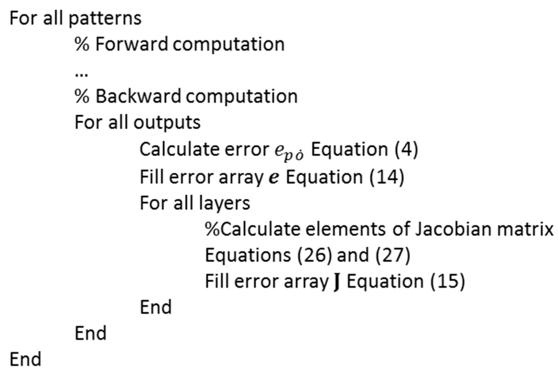
Calculation of Jacobian Matrix

According to Equations (4) and (15), the elements of Jacobian matrix can be calculated as:

$$\frac{\partial e_{p\dot{o}}}{\partial {\mathrm{w}}_i}=\frac{\partial \left(t_{p\dot{o}}-y_{p\dot{o}}\right)}{\partial {\mathrm{w}}_i}=-\frac{\partial y_{p\dot{o}}}{\partial {\mathrm{w}}_i}.$$

(23)

Considering an ANN of one hidden layer (Figure 2), the backpropagation is used in order to resolve the Equation (23). As shown in Figure 2, the superscript denotes the position of the layer in the network while the subscript describes the position of the neuron in the layer. In the weights, the double subscript indicates the neural connection in backpropagation order. The number of input and hidden neurons are defined by $N_x$ and $N_2$, respectively.

For a given pattern, the output $y_{p\dot{o}}$ could be calculated with backward computation:

$$y_{p\dot{o}}=f_{\dot{o}}^{\left(3\right)}({{\displaystyle \sum }}_{j=1}^{N_2}{\mathrm{n}}_j^{\left(2\right)}{\mathrm{w}}_{\dot{o}j}^{\left(2\right)}),$$

(24)

$$y_{p\dot{o}}=f_{\dot{o}}^{\left(3\right)}({{\displaystyle \sum }}_{j=1}^{N_2}{f}_j^{\left(2\right)}({{\displaystyle \sum }}_{i=1}^{N_x}{\mathrm{n}}_i^{\left(1\right)}{\mathrm{w}}_{ji}^{\left(1\right)}){\mathrm{w}}_{\dot{o}j}^{\left(2\right)}),$$

(25)

deriving Equations (24) and (25) with respect to ${\mathrm{w}}_{\dot{o}j}^{\left(2\right)}$ and ${\mathrm{w}}_{ji}^{\left(1\right)}$, respectively:

$$\frac{\partial y_{p\dot{o}}}{\partial {\mathrm{w}}_{\dot{o}j}^{\left(2\right)}}={\mathrm{d}}_{\dot{o}}^{\left(3\right)}{\mathrm{n}}_j^{\left(2\right)},$$

(26)

$$\frac{\partial y_{p\dot{o}}}{\partial {\mathrm{w}}_{ji}^{\left(1\right)}}={\mathrm{d}}_{\dot{o}}^{\left(3\right)}{\mathrm{d}}_j^{\left(2\right)}{\mathrm{w}}_{\dot{o}j}^{\left(2\right)}{\mathrm{n}}_i^{\left(1\right)}.$$

(27)

For the problem with patterns and outputs, the Jacobian and error matrices can be organized as the pseudocode shown in Figure 3.

Therefore, the training process using LM method can be planned as:

• Calculate the forward computation with initial weights (randomly generated).
• weights with Equation (22).
• the current total error. If the current total error is increased, then reset the weights to the previous values and increase $\mathsf{\mu }$ by a factor of 10. Then, go to Step 2. Otherwise, keep the new weights and decrease $\mathsf{\mu }$ by a factor of 10.
• Go to Step 2 until the current total error is smaller than the required value.

2.2. Wind Simulation

Among various simulation methods, the spectral representation methods appear to be the most widely used because they are fast and conceptually straightforward. Wind synthetic records can be generated from the spectral representation method proposed by Shinozuka and Jan [15]. Considering the case of $N_{\overline{p}}$ stationary stochastic processes $u_j\left(t\right)$, $j=1,2,3,\dots ,N_{\overline{p}}$ and discrete time $t=i\mathrm{∆}t$, $i=0,1,2,\dots ,N_s$, the mathematical expression for the generation of synthetic records is:

$$u_j\left(t\right)={{\displaystyle \sum }}_{k=1}^j{{\displaystyle \sum }}_{n=1}^{N_f}\left|{\overline{\mathrm{H}}}_{jk}\left({\omega }_n\right)\right|\sqrt{2\mathrm{∆}\omega }\cos \left[{\omega }_{n}t+{\theta }_{kn}\right],$$

(28)

where $u_j\left(t\right)$ is a signal with zero mean of size 1 × $N_{\mathrm{s}}$, representing the turbulent part of the longitudinal component at jth point in the space; ${\overline{\mathrm{H}}}_{jk}\left({\omega }_n\right)$ is an element of the lower triangular matrix $\overline{H}\left({\omega }_n\right)$ of size $N_{\overline{p}}$ × $N_{\overline{p}}$, which is defined by the Cholesky factorization process from the cross spectral density matrix; ${\theta }_{kn}$ is an element of the random phase angle matrix $\Theta$ of size $N_{\overline{p}}$ × $N_f$, with uniform distribution between [0, 2π]; ${\omega }_n$ is the discrete angular frequency (rad/s); $\mathrm{∆}\omega$ is the increment of angular frequency; and $N_f$ is the amount of values contained in the discrete spectral density function.

As it was shown in Equation (28), the calculation of the Shinozuka expression requires serial computing. In order to save computing time, an expression in matrix multiplication format based on the Shinozuka method is presented to perform the parallel computing taking into account the advantage of current multicore processors that can solve several vectors of the resulting matrix at the same time. The expression in array format is:

$$u=\sqrt{2\mathrm{∆}\omega }\left|\widehat{A}\right|\overline{X},$$

(29)

where $u$ is a matrix with size $N_{\overline{p}}$×$N_s$, and represents $N_{\overline{p}}$ stochastic process; $\widehat{A}$ is a matrix with size $N_{\overline{p}}$×($N_{\overline{p}}{N}_f$), defined by Equation (30); $\overline{X}$ is a matrix with size $\left(N_{\overline{p}}{N}_f\right)$×${\mathrm{N}}_s$, defined by Equation (31):

$$\widehat{A}={\left[\begin{array}{cccc}{\overline{H}}_{1,1}\left({\omega }_1\right)& {\overline{H}}_{2,1}\left({\omega }_1\right)& \dots & {\overline{H}}_{N_{\overline{p}},1}\left({\omega }_1\right)\\ {\overline{H}}_{1,2}\left({\omega }_1\right)& {\overline{H}}_{2,2}\left({\omega }_1\right)& \dots & {\overline{H}}_{N_{\overline{p}},2}\left({\omega }_1\right)\\ ⋮& ⋮& \ddots & ⋮\\ {\overline{H}}_{1,N_{\overline{p}}}\left({\omega }_1\right)& {\overline{H}}_{2,N_{\overline{p}}}\left({\omega }_1\right)& \dots & {\overline{H}}_{N_{\overline{p}},N_{\overline{p}}}\left({\omega }_1\right)\\ {\overline{H}}_{1,1}\left({\omega }_2\right)& {\overline{H}}_{2,1}\left({\omega }_2\right)& \dots & {\overline{H}}_{N_{\overline{p}},1}\left({\omega }_2\right)\\ ⋮& ⋮& \ddots & ⋮\\ {\overline{H}}_{1,N_{\overline{p}}}\left({\omega }_2\right)& {\overline{H}}_{2,N_{\overline{p}}}\left({\omega }_2\right)& \dots & {\overline{H}}_{N_{\overline{p}},N_{\overline{p}}}\left({\omega }_2\right)\\ ⋮& ⋮& \ddots & ⋮\\ {\overline{H}}_{1,1}\left({\omega }_{N_f}\right)& {\overline{H}}_{2,1}\left({\omega }_{N_f}\right)& \dots & {\overline{H}}_{N_{\overline{p}},1}\left({\omega }_{N_f}\right)\\ ⋮& ⋮& \ddots & ⋮\\ {\overline{H}}_{1,N_{\overline{p}}}\left({\omega }_{N_f}\right)& {\overline{H}}_{2,N_{\overline{p}}}\left({\omega }_{N_f}\right)& \dots & {\overline{H}}_{N_{\overline{p}},N_{\overline{p}}}\left({\omega }_{N_f}\right)\end{array}\right]}^{\mathrm{T}}$$

(30)

$$\overline{X}=\left[\begin{array}{cccc}\cos \left({\omega }_1{t}_1+{\theta }_{1,1}\right)& \cos \left({\omega }_1{t}_2+{\theta }_{1,1}\right)& \dots & \cos \left({\omega }_1{t}_{N_s}+{\theta }_{1,1}\right)\\ \cos \left({\omega }_1{t}_1+{\theta }_{1,2}\right)& \cos \left({\omega }_1{t}_2+{\theta }_{1,2}\right)& \dots & \cos \left({\omega }_1{t}_{N_s}+{\theta }_{1,2}\right)\\ ⋮& ⋮& \ddots & ⋮\\ \cos \left({\omega }_1{t}_1+{\theta }_{1,N_{\overline{p}}}\right)& \cos \left({\omega }_1{t}_2+{\theta }_{1,N_{\overline{p}}}\right)& \dots & \cos \left({\omega }_1{t}_{N_s}+{\theta }_{1,N_{\overline{p}}}\right)\\ \cos \left({\omega }_2{t}_1+{\theta }_{2,1}\right)& \cos \left({\omega }_2{t}_2+{\theta }_{2,1}\right)& \dots & \cos \left({\omega }_2{t}_{N_{\mathrm{s}}}+{\theta }_{2,1}\right)\\ ⋮& ⋮& \ddots & ⋮\\ \cos \left({\omega }_2{t}_1+{\theta }_{2,N_{\overline{p}}}\right)& \cos \left({\omega }_2{t}_2+{\theta }_{2,N_{\overline{p}}}\right)& \dots & \cos \left({\omega }_2{t}_{N_s}+{\theta }_{2,N_{\overline{p}}}\right)\\ ⋮& ⋮& \ddots & ⋮\\ \cos \left({\omega }_{N_f}{t}_1+{\theta }_{N_f,1}\right)& \cos \left({\omega }_{N_f}{t}_2+{\theta }_{N_f,1}\right)& \dots & \cos \left({\omega }_{N_f}{t}_{N_{\mathrm{s}}}+{\theta }_{N_f,1}\right)\\ ⋮& ⋮& \ddots & ⋮\\ \cos \left({\omega }_{N_f}{t}_1+{\theta }_{N_f,N_{\overline{p}}}\right)& \cos \left({\omega }_{N_f}{t}_2+{\theta }_{N_f,N_{\overline{p}}}\right)& \dots & \cos \left({\omega }_{{\mathrm{N}}_f}{t}_{N_s}+{\theta }_{N_f,N_{\overline{p}}}\right)\end{array}\right]$$

(31)

Cross-Spectral Density Matrix

The cross-spectral density matrix describes the influence of the turbulence components at two points at a given frequency. This influence is due to the spatial dimension of the vortices in the wind field. Considering Cholesky, if the cross spectral density matrix ${\mathit{S}}^0\left(\omega \right)$ is symmetric positive definite, then ${\mathit{S}}^0\left(\omega \right)$ can be decomposed as [1]:

$${\mathit{S}}^0\left(\omega \right)=\overline{H}\left(\omega \right){\overline{H}}^{\mathrm{T}}\left(\omega \right),$$

(32)

where ${\mathit{S}}^0\left(\omega \right)$ is the cross spectral density matrix for angular frequency ω; and $\overline{H}\left(\omega \right)$ is a lower triangular matrix.

The process of Cholesky factorization is as follows:

$$\begin{gathered} {\overline{\mathrm{H}}}_{11}\left(\omega \right)=S_{11}^0{\left(\omega \right)}^{1/2} \\ {\overline{\mathrm{H}}}_{21}\left(\omega \right)=S_{21}^0\left(\omega \right)/{\overline{\mathrm{H}}}_{11}\left(\omega \right) \\ {\overline{\mathrm{H}}}_{22}\left(\omega \right)=(S_{22}^0\left(\omega \right)-{\overline{\mathrm{H}}}_{21}{\left(\omega \right)}^2{)}^{1/2} \\ {\overline{\mathrm{H}}}_{31}\left(\omega \right)=S_{31}^0\left(\omega \right)/{\overline{\mathrm{H}}}_{11}\left(\omega \right) \\ ⋮ \\ {\overline{\mathrm{H}}}_{jk}\left(\omega \right)=\left(S_{jk}^0\left(\omega \right)-{{\displaystyle \sum }}_{l=1}^{k-1}{\overline{\mathrm{H}}}_{jl}\left(\omega \right){\overline{\mathrm{H}}}_{kl}\left(\omega \right)\right)/{\overline{\mathrm{H}}}_{kk}\left(\omega \right) \\ {\overline{\mathrm{H}}}_{kk}\left(\omega \right)=(S_{kk}^0\left(\omega \right)-{{\displaystyle \sum }}_{l=1}^{k-1}{\overline{\mathrm{H}}}_{kl}{\left(\omega \right)}^2{)}^{1/2}. \end{gathered}$$

(33)

For two points with vertical separation$r_y$, the $S_{ij}^0\left(\omega \right)$ corresponding elements are obtained by the cross-spectral density function $S_{uu}\left(z_i,z_j,n\right)$:

$$S_{uu}\left(z_i,z_j,n\right)=\sqrt{S_u\left(z_i,n\right)S_u\left(z_j,n\right)}\sqrt{\mathrm{coh}\left(r_y,n\right)},$$

(34)

where $S_{uu}\left(z_i,z_j,n\right)$ is the cross spectral density function for two longitudinal turbulent components at space points $z_1$ and $z_2$; $S_u\left(z_i,n\right)$ is the single power density spectrum at $z_i$, defined in Equation (38); $\sqrt{\mathrm{coh}\left(r_y,n\right)}$ is the root-coherence function, defined in Equation (35); $n$ is the frequency in Hz. The root-coherence function defines the static dependence between two turbulent components at two different points. This function tends to zero when the separation $r_y$ increases; in other words, the cross-influence of the wind turbulent is inversely proportional to the separation. Davenport [19] suggested an exponential expression as root-coherence function:

$$\sqrt{\mathrm{coh}\left(r_y,n\right)}=e^{\left(-C_y{r}_y\frac{n}{\overline{U}}\right)},$$

(35)

where $\overline{U}$ is the average speed between two points, calculated as $1/2\left[\overline{U}\left(z_i\right)+\overline{U}\left(z_j\right)\right]$; $C_y$ is a non-dimensional decay constant, whose typical value is 10.

The variation of mean wind speed to different levels of height can be calculated with an expression known as power law:

$$\overline{U}\left(z\right)={\mathrm{f}}_s\overline{b}{\overline{\mathrm{U}}}_{10,\mathrm{II}}{\left(\frac{z}{10}\right)}^{\overline{\alpha }},$$

(36)

where ${\mathrm{f}}_s$ is a time scale factor, according to Mackey [20] ${\mathrm{f}}_s=0.702$ in order to scale 3-s to 10-min of mean wind speeds; $\overline{b}$ is the roughness factor, defined in

Table 1. Terrain categories and terrain parameters based in Eurocode [22].

Terrain Category	${\mathit{z}}_0$ (m)	$\overline{\mathit{b}}$
I—Lakes or flat and horizontal area with negligible vegetation and without obstacles	0.01	1.17
II—Area with low vegetation such as grass and isolated obstacles (trees, buildings) with separations of at least 20 obstacle heights	0.05	1.00
III—Area with regular cover of vegetation or buildings or with isolated obstacles with separations of maximum 20 obstacle heights (such as villages, suburban terrain, permanent forest)	0.30	0.77
IV—Area in which at least 15% of the surface is covered with buildings and their average height exceeds 15 m	1.00	0.55

; ${\overline{\mathrm{U}}}_{10,\mathrm{II}}$ is the basic wind speed, and it is a mean wind speed taking at reference height 10 m and terrain category II; $\overline{\alpha }$ is the exponent, defined in Equation (37).

According to Counihanm [21], the exponent $\overline{\alpha }$ depends on the characteristics of roughness, and can be calculated with the following equation:

$$\overline{\alpha }=0.096{\log }_{10}{z}_0+0.016{\left({\log }_{10}{z}_0\right)}^2+0.24.$$

(37)

The power spectral density function used in this paper is the von Karman–Harris model [23,24], which has shown a very good approach at high frequency with application to wind codes [25], and it is considering the most mathematically correct wind spectrum according to [26]. The mathematical form of von Karman-Harris model is:

$$S_u\left(z,n\right)=\frac{4\left({\sigma }_u^2\right)L_u\left(z\right)/\overline{U}\left(z\right)}{{\left[1+70.8{\left(\frac{n{L}_u\left(z\right)}{\overline{U}\left(z\right)}\right)}^2\right]}^{5/6}},$$

(38)

where $L_u\left(z\right)$ is the integral length scale; and ${\sigma }_u$ is standard deviations for the turbulence components.

The standard deviations of wind speed are related with the turbulence intensity. The turbulence intensity is the most basic measure of turbulence, and it is defined by the ratio of the standard deviation of the wind speed to the mean wind speed:

$$I_u\left(z\right)={\sigma }_u/\overline{U}\left(z\right).$$

(39)

The turbulence intensity can be estimated by the following empirical expression [22]:

$$I_u\left(z\right)=\frac{1}{\ln \left(z/z_0\right)}.$$

(40)

The integral length scales are a measure of the sizes of the vortices in the wind or, in other words, the average size of a gust in a given direction [26]. In wind codes, a typical expression in order to estimate the integral length scales is [22]:

$$L_u\left(z\right)=300{\left(\frac{z}{200}\right)}^v,$$

(41)

where the exponent $v$ depends on the roughness length $z_0$, and it can be calculated by:

$$v=0.67+0.05\ln \left(z_0\right).$$

(42)

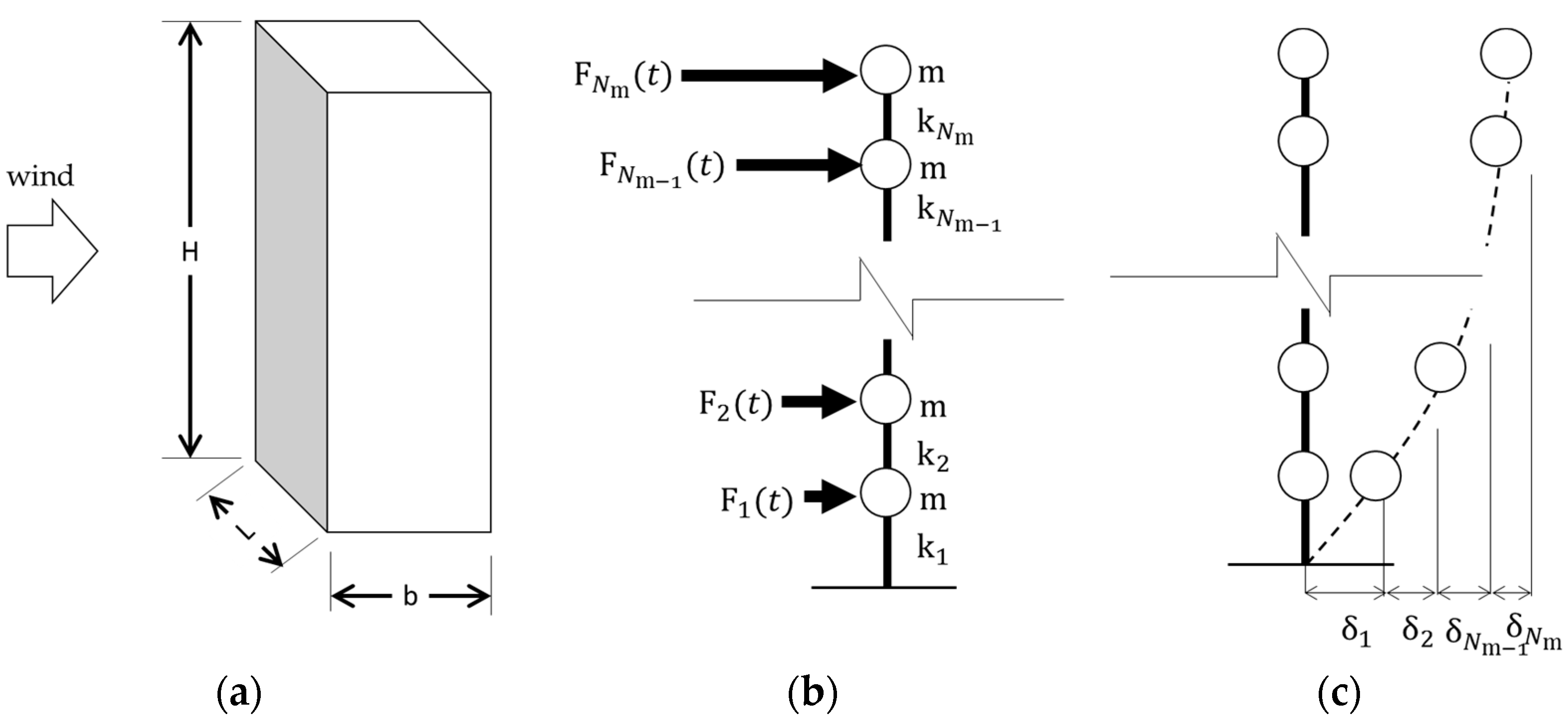
2.3. Dynamic Response

The Newmark method is one of the numerical integration methods most frequently used in structural dynamic analysis; software packages such as OpeenSees (v2002, CA, USA), Ruaumoko (v2004, Christchurch, New Zealand) and SAP2000 (v2012, CA, USA) [27,28,29] include routines of dynamic analysis by this method. This procedure is based on two types of assumptions in order to simplify and solve the differential equations of motion. The assumptions are focused on determining the acceleration between two time instants, which may be linear or a constant mean value. The idealization of a prismatic building as shear-frame or shear-building (Figure 4) can be represented by a Multi-Degree-of-Freedom (MDOF) system [30]. The governing equation of motion for MDOF systems subjected to external forces can be given in a matrix form as next:

$$M\ddot{\mathit{d}}+C\dot{\mathit{d}}+K\mathit{d}=F,$$

(43)

where $M$, $C$ and $K$ are the mass, damping and stiffness matrices, respectively, 𝒅, $\dot{\mathit{d}}$ and $\ddot{\mathit{d}}$ are the displacement, velocity and acceleration vectors; and $F$ is a matrix with the force vectors.

The matrix form of the mass and stiffness matrices for a MDOF structure (Figure 4b) with shear resistant are:

$$M=\left[\begin{array}{ccccc}\mathrm{m}& 0& \cdots & \cdots & 0\\ 0& \mathrm{m}& 0& \cdots & 0\\ \cdots & 0& \cdots & 0& \cdots \\ 0& \cdots & 0& \mathrm{m}& 0\\ 0& \cdots & \cdots & 0& \mathrm{m}\end{array}\right];\hspace{1em}K=\left[\begin{array}{ccccc}{\mathrm{k}}_1+{\mathrm{k}}_2& -{\mathrm{k}}_2& \cdots & \cdots & 0\\ -{\mathrm{k}}_2& {\mathrm{k}}_2+{\mathrm{k}}_3& \cdots & \cdots & 0\\ \cdots & \cdots & \cdots & \cdots & \cdots \\ 0& \cdots & \cdots & {\mathrm{k}}_{N_{\mathrm{m}-1}}-{\mathrm{k}}_{N_{\mathrm{m}}}& -{\mathrm{k}}_{N_{\mathrm{m}}}\\ 0& \cdots & \cdots & -{\mathrm{k}}_{N_{\mathrm{m}}}& {\mathrm{k}}_{N_{\mathrm{m}}}\end{array}\right]$$

(44)

. .

The form of the damping matrix $C$ depends on the damping characteristic of the structure, which can be classical or nonclassical damping. The classical damping is an appropriate idealization if similar damping mechanisms are distributed throughout the structure, e.g., a multistory building with a similar structural system and structural materials over its height [30]. In this work, the Rayleigh Damping method is used in order to build a classical matrix $C$. The damping matrix can be approached by the following equation of Rayleigh:

$$c=a_{0}M+a_{1}K,$$

(45)

where $a_0$ and $a_1$ Rayleigh coefficient and could be estimated by:

$$a_0=\zeta \frac{2{\omega }_i{\omega }_j}{{\omega }_i+{\omega }_j}; a_1=\zeta \frac{2}{{\omega }_i+{\omega }_j},$$

(46)

where $\zeta$ is the damping ratio for the first mode; and ${\omega }_i$ and ${\omega }_j$ are two angular frequencies that correspond to two adjacent vibration modes.

Assuming a free vibration system without damping, the equation of motion is as follows:

$$M\ddot{\mathit{d}}+K\mathit{d}=\mathbf{0}.$$

(47)

Substituting $\mathit{d}=\Phi q\left(t\right)=\Phi \sin \left(\mathsf{\omega }\mathrm{t}\right)$ in Equation (47), the following expression is an eigenvalue problem:

$$K\Phi =M\Phi {\mathsf{\omega }}^2,$$

(48)

where $\Phi$ is modal matrix that represents the deflected shape for each vibration modes; $q$ is a vector for each instant time and represents the modal coordinates; and $\omega$ is a diagonal matrix with the angular frequency of vibration.

Rewriting the equation of motion to the modal form and multiplying all expressions by ${\Phi }^{\mathrm{T}}$:

$$\overline{M}\ddot{q}+\overline{C}\dot{q}+\overline{K}q=\overline{F},$$

(49)

where $\overline{M}={\Phi }^{\mathrm{T}}M\Phi$, $\overline{C}={\Phi }^{\mathrm{T}}C\Phi$, $\overline{K}={\Phi }^{\mathrm{T}}K\Phi$ and $\overline{F}={\Phi }^{\mathrm{T}}F$ are modal transformation matrices corresponding to the mass, damping, stiffness, and forces matrices, respectively.

The procedure of the Newmark method for MDOF structures is shown in

Table 2. Procedure of the Newmark method for multi-degrees of freedom systems.

Step-by-step procedure:
Initial calculations:
1.1 $\widehat{K}=\overline{K}+\frac{\gamma }{\beta \Delta t}\overline{C}+\frac{1}{\beta {\left(\Delta t\right)}^2}\overline{M}$
1.2 $\mathrm{a}=\frac{1}{\beta \Delta t}\overline{M}+\frac{\gamma }{\beta }\overline{C},\mathrm{b}=\frac{1}{2\beta }\overline{M}+\Delta t\left(\frac{\gamma }{2\beta }-1\right)\overline{C}$
Calculations for each time step $i$
2.1 ${\overline{F}}_i={\Phi }^{\mathrm{T}}{F}_i$
2.2 $\mathbf{\Delta }{\widehat{F}}_i=\mathbf{\Delta }{\overline{F}}_i+\mathrm{a}{\dot{q}}_{\mathit{i}}+\mathrm{b}{\ddot{q}}_{\mathit{i}}$
2.3 $\mathbf{\Delta }{q}_i={\widehat{K}}^{-\mathbf{1}}\mathbf{\Delta }{\widehat{F}}_i$
2.4 $\mathbf{\Delta }{\dot{q}}_i=\frac{\gamma }{\beta \Delta t}\mathbf{\Delta }{q}_i-\frac{\gamma }{\beta }{\dot{q}}_{\mathit{i}}+\Delta t\left(1-\frac{\gamma }{2\beta }\right){\ddot{q}}_{\mathit{i}}$
2.5 $\mathbf{\Delta }{\ddot{q}}_i=\frac{1}{\beta {\left(\Delta t\right)}^2}\mathbf{\Delta }{q}_i-\frac{1}{\beta \Delta t}{\dot{q}}_{\mathit{i}}-\frac{1}{2\beta }{\ddot{q}}_{\mathit{i}}$
2.6 $q_{i+1}=q_i+\mathbf{\Delta }{q}_i,{\dot{q}}_{i+1}={\dot{q}}_i+\mathbf{\Delta }{\dot{q}}_i,{\ddot{q}}_{i+1}={\ddot{q}}_i+\mathbf{\Delta }{\ddot{q}}_i$
2.7 ${\mathit{d}}_{i+1}=\Phi q_{i+1}$
Repetition for the next time step. Replace $i$ by $i+1$ and implement Steps 2.1 and 2.7 for the next time step.

, see Chopra [30], where $i$ indicates the time step. The factors $\beta$ and $\gamma$ are constant values taking $\beta =1/4$ and $\gamma =1/2$ for the case of average acceleration and $\beta =1/6$ y $\gamma =1/2$ for the linear acceleration.

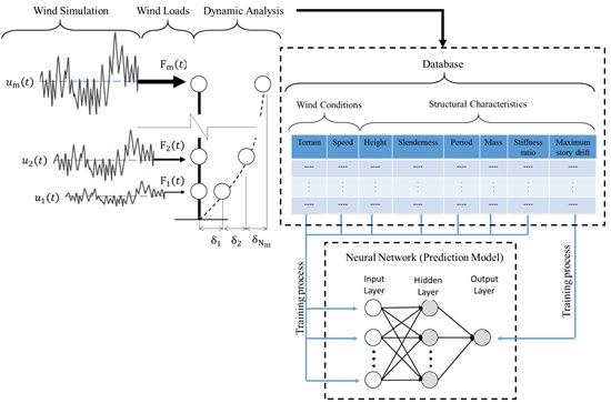
3. Application of Theoretical Framework

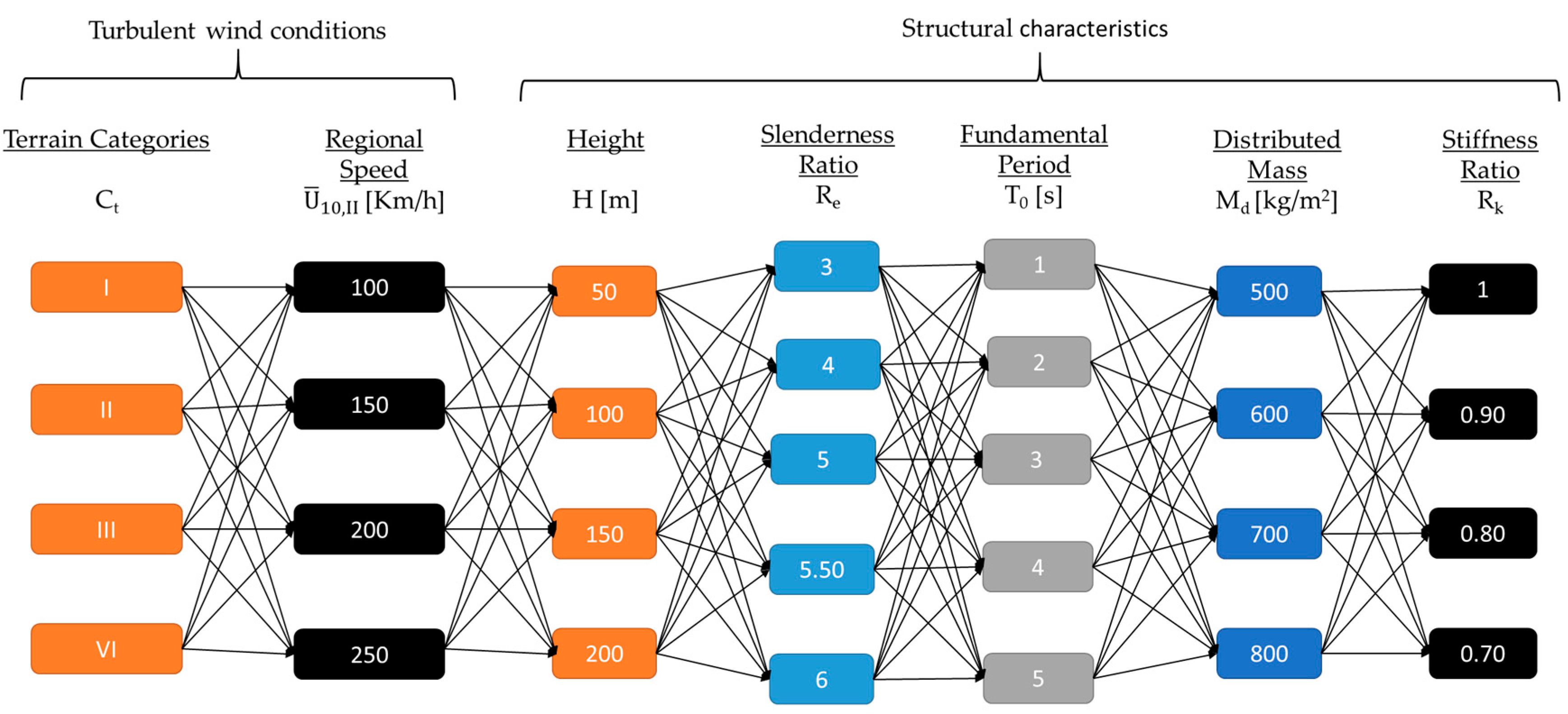
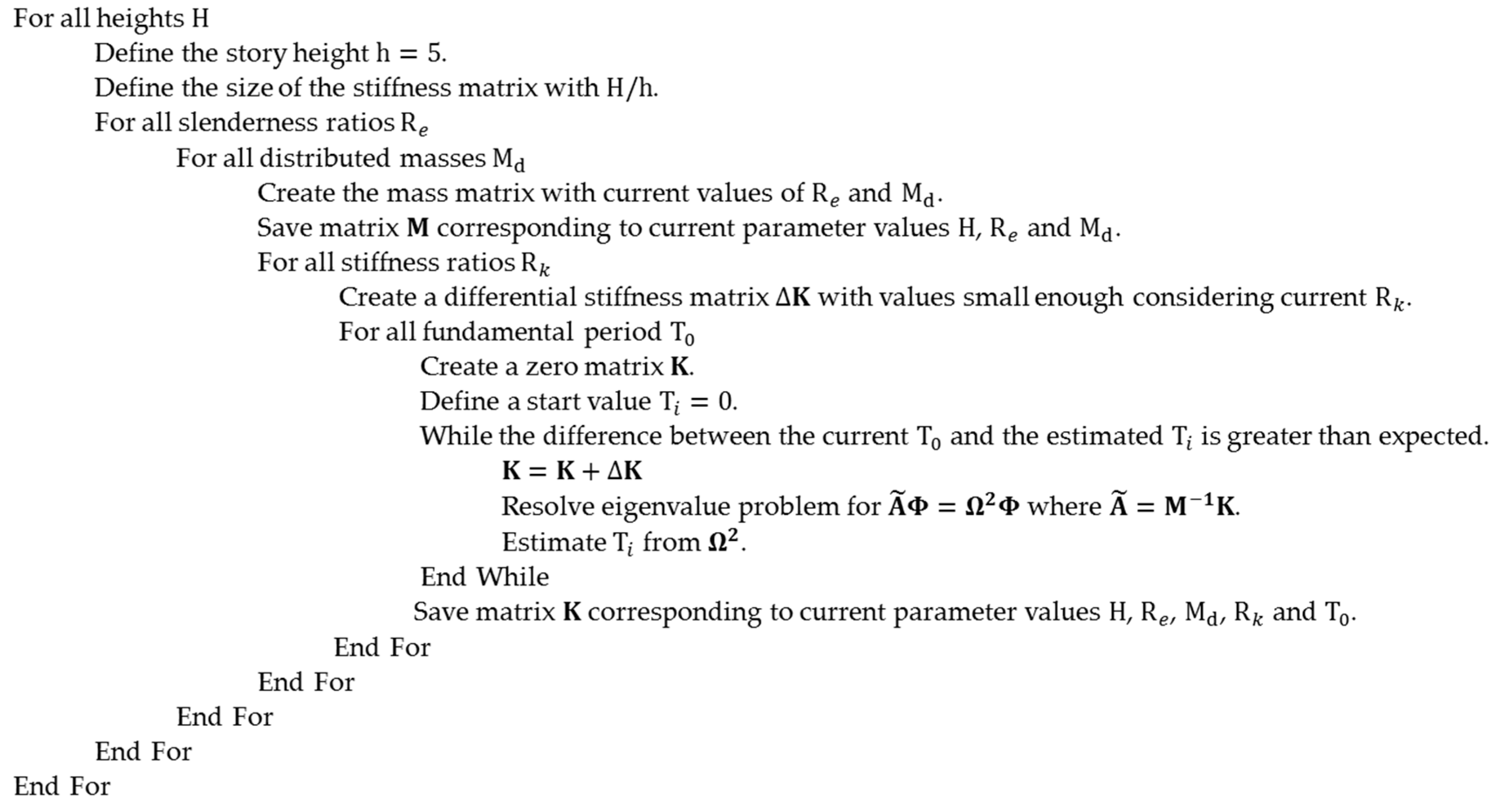
3.1. Data Generation

In this paper, several steel shear-buildings discretized as MDOF structures with different structural vibration period T₀ were analyzed using wind loads from synthetic records of 10 min. The case studies are defined by the combinations of some parameters that consider diverse wind conditions and structural characteristics (see Figure 5). The range of values for each parameter was selected to cover a considerable number of sensitive structures to the dynamic effects of the wind. The values of basic wind speed or regional speed are presented in 3-s gust wind speeds because this is more common in this type of design; however, the time scale factor was considered for 10 min. The slenderness relation is defined as ${\mathrm{R}}_e=\mathrm{H}/\mathrm{b}$, where $\mathrm{H}$ is the total height of the structure and $\mathrm{b}$ is the plane dimension parallel to the direction of the wind (see Figure 4a). The stiffness ratio corresponds to the reduction of the stiffness along the height between the first and the last story level, i.e., ${\mathrm{R}}_k=k_{{\mathrm{N}}_{\mathrm{m}}}/k_1$ (see Figure 4b). The distributed mass represents the mass concentration per unit area for each floor, and this parameter defines the lumped mass $\mathrm{m}$ of each story level.

The dynamic loads are generated from synthetic records, where the turbulent parts of the longitudinal components are obtained by the Shinozuka method. According to Bernoulli, the wind is air mass with kinetic energy. It can be expressed in terms of pressure or force acting on a contact area; the mathematical form for a structure is [31]:

$${\mathrm{F}}_j\left(t\right)=\frac{1}{2}{C}_d\rho A_j{\left({\mathrm{U}}_j\left(t\right)-{\dot{d}}_j\left(t\right)\right)}^2$$

(50)

where ${\mathrm{F}}_j\left(t\right)$ is the wind force on the j-th floor; $C_d$ is the drag coefficient, for rectangular prismatic $C_d\approx 1$ [31], which is used to quantify the drag or resistance of an object in a fluid environment; $\rho$ is the density of the air, for this study $\rho =1.25$ kg/m³; $A_j$ is the contact area on the j-th floor; and ${\mathrm{U}}_j\left(t\right)$ is the longitudinal component of the wind. It is defined as the sum of the mean velocity and its corresponding turbulent part ${\mathrm{U}}_j\left(t\right)={\overline{\mathrm{U}}}_j+u_j\left(t\right)$; ${\dot{d}}_j\left(t\right)$ is the velocity of the mass lumped on the $j$th floor.

The stiffness matrix, required for the dynamic analysis, was calculated by an iterative process, where the all parameters of structure definition are involved. The pseudo-code used for the creation of the mass and stiffness matrices is shown in Figure 6.

With the loads calculated and the structures defined, the Newmark method is used to obtain the response of 1600 structures and each one is exposed to 16 scenarios of turbulent wind. Figure 7 shows the behavior of the maximum story drift for a certain group of structures and wind conditions. It is observed that the maximum story drift is directly proportional to the fundamental period and the wind speed and inversely proportional to the terrain roughness. The behavior of these surfaces is appropriate according to the variations of the parameters.

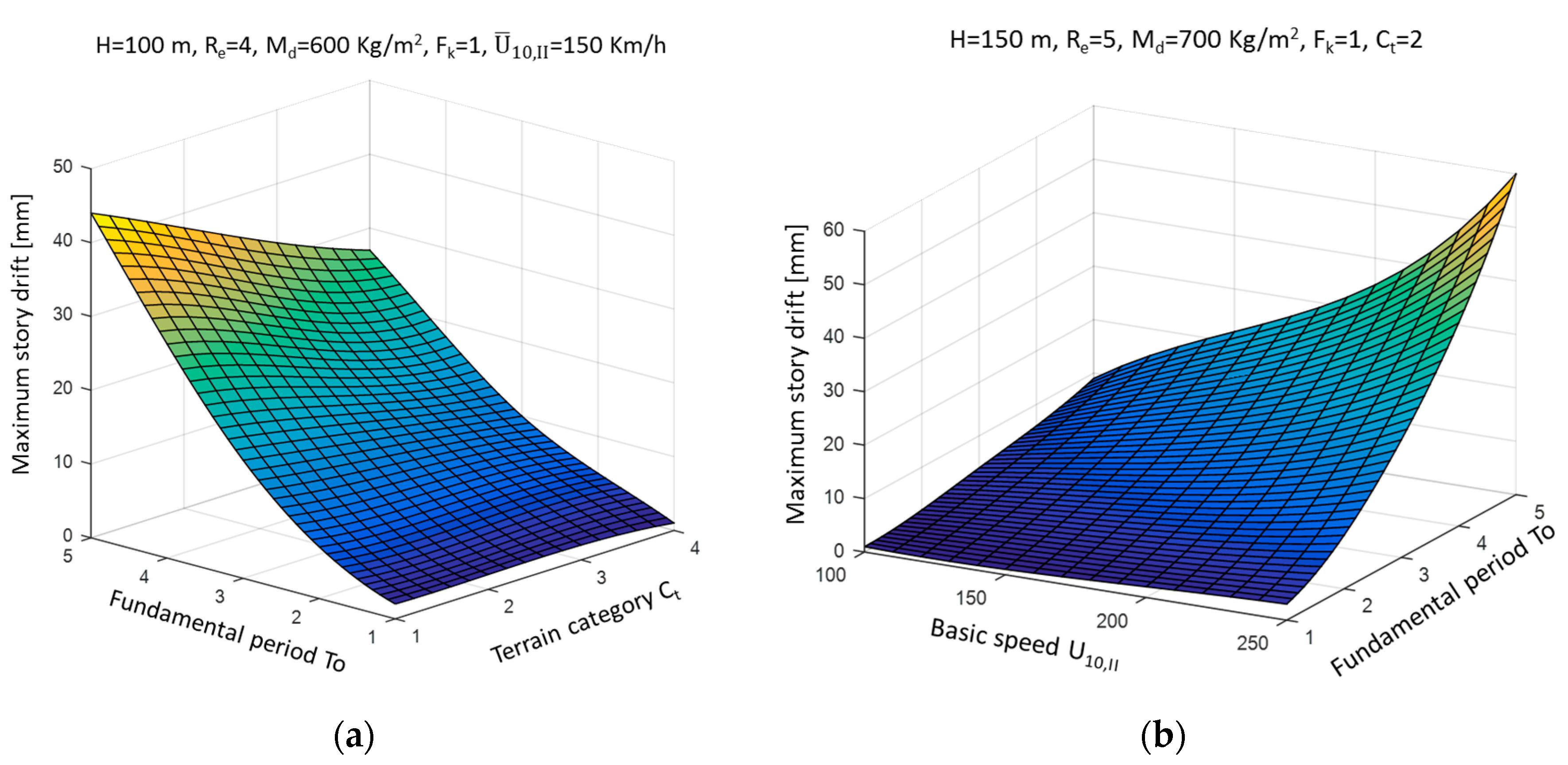
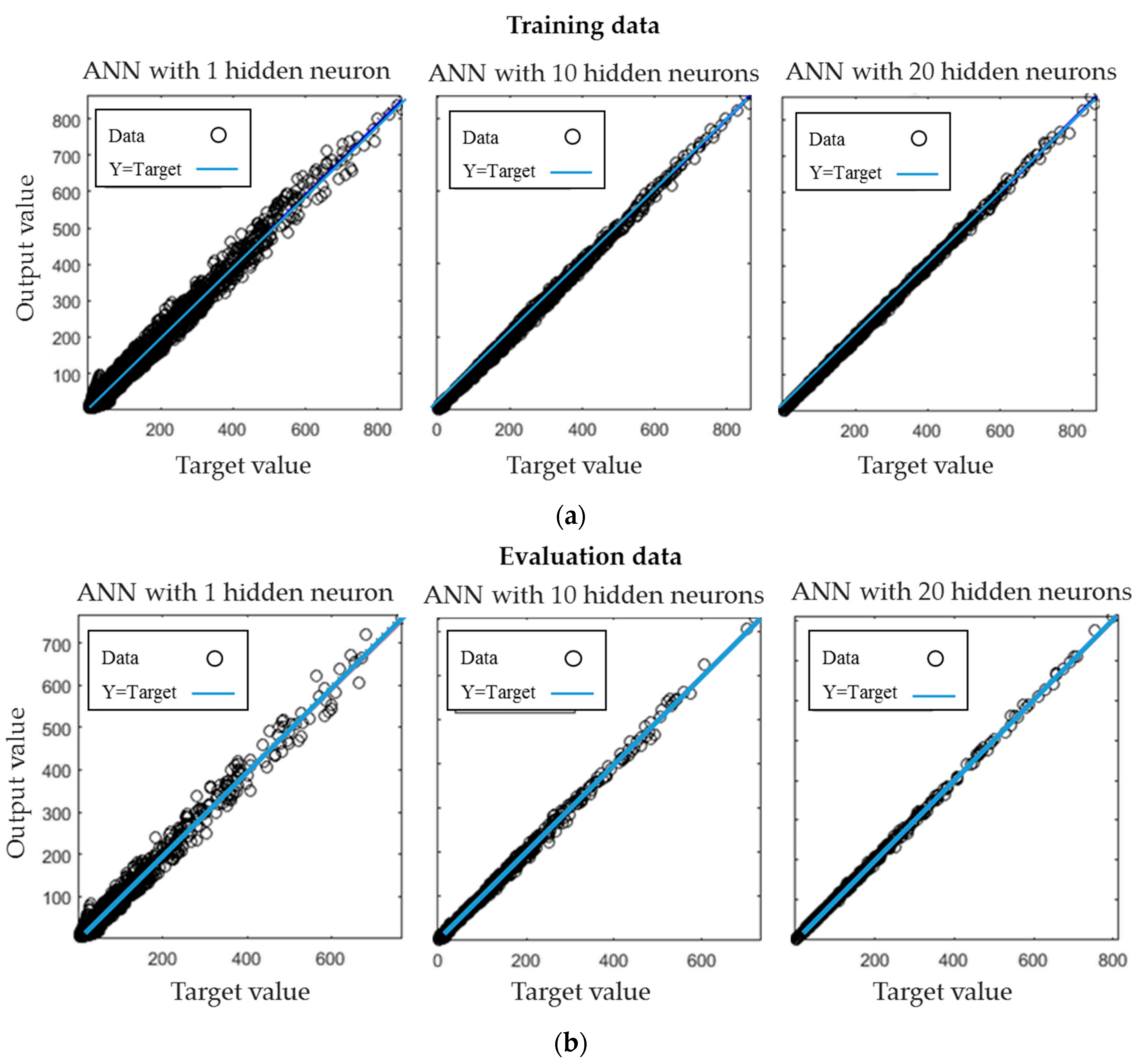
3.2. Results of Network Trainings

The maximum story drifts obtained for each case study are used as the dataset for the network training process by the LM method. For the network architecture, the parameters of height, slenderness ratio, fundamental period, distributed mass, stiffness ratio, terrain categories and basic wind speed represent seven input values needed to estimate an output, which tends to predict the maximum story drifts. With the aim of evaluating the efficiency of the network against new data (not analyzed), a small percentage (15%) taken randomly of the dataset is excluded in the training process.

Table 3. Results of network trainings with different number of neurons in the hidden layer.

Hidden Neurons	Training Data	Evaluation Data	Training Iterations	MSE Training Data	MSE Evaluation Data
1	21,760	3840	1000	101.72	108.96
2	21,760	3840	1000	65.48	62.96
5	21,760	3840	1000	23.92	29.22
10	21,760	3840	1000	8.89	9.06
12	21,760	3840	1000	5.73	5.88
20	21,760	3840	1000	2.59	2.91
30	21,760	3840	1000	2.05	2.21

shows the mean square error (MSE) generated for the ANNs with different number of neurons in the hidden layer. It is observed that the error is reduced when the number of neurons in the hidden layer increases. A larger number of hidden neurons allows for modeling any variation in the data; however, the decrees of the error are not significant from 20 hidden neurons.

Figure 8 shows the relation between the target values and the output values of the ANNs with 1, 10 and 20 hidden neurons considering training and evaluation data. It is observed that the increase in the number of neurons in the hidden layer helps to improve the linear relation close to 99%.

The cross-validation is a technique to evaluate the independence of the results of a prediction model with relation to the training and testing dataset selected.

Table 4. Cross-validation of the ANN with 20 hidden neurons.

Validation Iterations	MSE Training Data	MSE Evaluation Data
Iteration 1	3.51	3.71
Iteration 2	2.86	2.94
Iteration 3	2.24	3.01
Iteration 4	2.58	2.82
Iteration 5	3.99	3.65
Iteration 6	3.42	3.58
Iteration 7	2.79	2.74
Iteration 8	3.21	3.31
Iteration 9	2.49	2.58
Iteration 10	2.73	3.00

shows the cross-validation of the ANN with 20 hidden neurons using, in each iteration, different training and evaluation dataset taken randomly that represent the 85 and 15 percent, respectively. Small variations of MSE between each dataset and iteration are observed. Therefore, the dataset selected generates in an independent way results very close to each other.

Table 5. Memory and computer time in order to process the tasks of the case: H = 150 m, R_e = 5, M_d = 500 Kg/m², F_k = 1, T₀ = 3 s, C_t = 2, ${\overline{\mathrm{U}}}_{10,\mathrm{II}}$ = 150 Km/h.

Procedure	Phase	Memory (MB)	Computer Time (s)
Standard	Wind Simulation	6850	386.41
	Calculate stiffness matrix	13	5.93
	Dynamic analyse	29	24.07
ANN with 20 hidden neurons	Trainging	424	934.15
	Execute	0.01	0.001

shows the memory and computer time required in the tasks of computational processing for the case H = 150 m, R_e = 5, M_d = 500 Kg/m², F_k = 1, T₀ = 3 s, C_t = 2, ${\overline{\mathrm{U}}}_{10,\mathrm{II}}$ = 150 Km/h. A greater computer time in the training network is observed than the sum of all phases of the standard procedure; however, once the network has been trained, it is prepared to respond to many possible cases of immediately and using little memory.

4. Conclusions

The maximum story drift of 1600 shear-buildings discretized as MDOF structures were obtained. The Shinozuka and Newmark methods were employed to simulate the synthetic wind records and to obtain the dynamic response of the structures, respectively. The wind loads necessary to compute the dynamic response were developed from wind synthetic records considering 16 turbulent wind conditions. The Artificial Neural Networks (ANNs) were used to generate a computational model capable of estimating the maximum story drift of 25,600 case studies. The Levenberg–Marquardt (LM) method is applied in the process of network training. The parameters of height, slenderness ratio, fundamental period, distributed mass, stiffness ratio, terrain categories and basic wind speed represented the input values in the ANNs. Seven network architectures with 1 to 30 neurons in one hidden layer were studied to evaluate its predictive efficiency. It is observed that errors decrease when the number of neurons in the hidden layer increases. Nevertheless, the decreases of the errors are not significant from 20 hidden neurons. The cross-validation with 10 iterations suggested independence acceptable between the dataset selected for training and the results. The study of computer times required in the tasks of computational processing indicated a major processing time in training networks compared to a standard procedure for a specific case; nevertheless, once the network has been trained, it is prepared to respond to many possible cases of immediately and using little computational memory. Finally, it was demonstrated that with the use of ANNs and the LM method, it is possible to obtain a computational model capable of predicting with a good relationship the maximum story drift of MDOF structures.

References

1. Veers, P.S. Three-Dimensional Wind Simulation; Sandia National Labs: Albuquerque, NM, USA, 1988. [Google Scholar]
2. Chay, M.T.; Albermani, F.; Wilson, R. Numerical and analytical simulation of downburst wind loads. Eng. Struct. 2006, 28, 240–254. [Google Scholar] [CrossRef]
3. Bojórquez, E.; Payán-Serrano, O.; Reyes-Salazar, A.; Pozos, A. Comparison of spectral density models to simulate wind records. KSCE J. Civ. Eng. 2016, 1, 1–8. [Google Scholar] [CrossRef]
4. Davenport, A.G. Gust loading factors. J. Struct. Div. 1967, 93, 11–34. [Google Scholar] [CrossRef]
5. Davenport, A.G. The representation of the dynamic effects of turbulent wind by equivalent static wind loads. Proceedings of International Symposium on Structural Steel, Chicago, IL, USA, 1985; pp. 1–13. [Google Scholar]
6. Chen, X.; Kareem, A. Equivalent static wind loads on buildings: New model. J. Struct. Eng. 2004, 130, 1425–1435. [Google Scholar] [CrossRef]
7. Repetto, M.P.; Solari, G. Equivalent static wind actions on vertical structures. J. Wind Eng. Ind. Aerodyn. 2004, 92, 335–357. [Google Scholar] [CrossRef]
8. Hecht-Nielsen, R. Neurocomputer applications. Neural Comput. 1989, 41, 445–453. [Google Scholar] [CrossRef]
9. Conte, J.P.; Durrani, A.J. Seismic Response modeling of multi-story buildings using neural networks. J. Intell. Mater. Syst. Struct. 1994, 5, 392–402. [Google Scholar] [CrossRef]
10. Chakraverty, S.; Gupta, P.; Sharma, S. Neural network-based simulation for response identification of two-storey shear building subject to earthquake motion. Neural Comput. Appl. 2010, 19, 367–375. [Google Scholar] [CrossRef]
11. Bojórquez, J.; Ruiz, S.; Bojórquez, E.; Reyes-Salazar, A. Probabilistic seismic response transformation factors between SDOF and MDOF systems using artificial neural networks. J. Vibroeng. 2016, 18, 2248–2262. [Google Scholar] [CrossRef]
12. Roy, D.; Dash, M.K. Explorations of a family of stochastic Newmark methods in engineering dynamics. Comput. Methods Appl. Mech. Eng. 2005, 194, 4758–4796. [Google Scholar] [CrossRef]
13. Krenk, S. Energy conservation in Newmark based time integration algorithms. Comput. Methods Appl. Mech. Eng. 2006, 195, 6110–6124. [Google Scholar] [CrossRef]
14. Bourihane, O.; Braikat, B. Dynamic analysis of a thin-walled beam with open cross section subjected to dynamic loads using a high-order implicit algorithm. Eng. Struct. 2016, 120, 133–146. [Google Scholar] [CrossRef]
15. Shinozuka, M.; Jam, C.M. Digital simulation of random processes and its applications. J. Sound Vib. 1972, 25, 111–128. [Google Scholar] [CrossRef]
16. Rossi, R.; Lazzari, M.; Vitaliani, R. Wind field simulation for structural engineering purposes. Int. J. Num. Method Eng. 2004, 61, 738–763. [Google Scholar] [CrossRef]
17. Levenberg, K. A method for the solution of certain problems in least squares. Q. Appl. Math. 1944, 5, 164–168. [Google Scholar] [CrossRef]
18. Suratgar, A.A.; Tavakoli, M.B.; Hoseinabadi, A. Modified Levenberg–Marquardt method for neural networks training. World Acad. Sci. Eng. Technol. 2005, 6, 46–48. [Google Scholar]
19. Davenport, A.G. The spectrum of horizontal gustiness near the ground in high winds. Q. J. R. Meteorol. Soc. 1961, 87, 194–211. [Google Scholar] [CrossRef]
20. Mackey, S. Gust Factors. In Proceedings of the Seminar USA-Japan Research Seminar: Wind Loads on Structures; University of Hawaii: Honolulu, HI, USA, 1970; pp. 191–202. [Google Scholar]
21. Counihan, J. Adiabatic atmospheric boundary layers: A review and analysis of data from the period from 1880–1972. Atmos. Environ. 1967, 9, 871–905. [Google Scholar] [CrossRef]
22. Hirt, M.A. Eurocode 1. Basis of design and action on structures Part 1–4. Schweizer Ingenieur Architekt 1993, 16–17, 273–275. [Google Scholar]
23. Von Karman, T. Progress in the statistical theory of turbulence. Proc. Natl. Acad. Sci. USA 1948, 34, 530–539. [Google Scholar] [CrossRef] [PubMed]
24. Harris, R.I. On the Spectrum and Auto-correlation Function of Gustiness in High Winds; Electrical Research Association: Leatherhead, UK, 1968. [Google Scholar]
25. Lungu, D.; van Gelder, P. Characteristics of wind turbulence with applications to wind codes. In Proceedings of the 2nd European & African Conference on Wind Engineering, Genova, Italy, 22–26 June 1997; pp. 1271–1277. [Google Scholar]
26. Xu, Y.L. Wind Effects on Cable-Supported Bridges; John Wiley and Sons: New York, NY, USA, 2013. [Google Scholar]
27. McKenna, F.; Fenves, G.L.; Scott, M. Open System for Earthquake Engineering Simulation (OpenSees); University of California: Berkeley, CA, USA, 2002. [Google Scholar]
28. Carr, A.J. RUAUMOKO-2D Inelastic Time-History Analysis of Two Dimensional Framed Structures; Department of Civil Engineering, University of Canterbury: Christchurch, New Zealand, 2004. [Google Scholar]
29. Computer and Structure, Inc. SAP2000 Documentation, Release 15.1.0; University Ave: Berkeley, CA, USA, 2012. [Google Scholar]
30. Chopra, A. Dynamics of Structures: Theory and Applications to Earthquake Engineering; Prentice Hall: Englewood Cliffs, NJ, USA, 2014. [Google Scholar] [CrossRef]
31. Holmes, J.D. Wind Loading of Structures; CRC Press: Boca Raton, FL, USA, 2015. [Google Scholar]
Figure 1. Graphic description of an Artificial Neural Network (ANN) (a) topology of multilayer perceptron (forward propagation); (b) internal process for each neuron.
Applsci 07 00563 g001
Figure 2. Perceptron with one hidden layer.
Applsci 07 00563 g002
Figure 3. Pseudocode for Jacobian matrix.
Applsci 07 00563 g003
Figure 4. (a) Prismatic buildings with rectangular cross section; (b) multi-degree-of-freedom structure; (c) story drift.
Applsci 07 00563 g004
Figure 5. Parameters for definition of the structures and dynamic wind loads.
Applsci 07 00563 g005
Figure 6. Pseudo-code in order to calculate mass and stiffness matrices.
Applsci 07 00563 g006
Figure 7. Maximum story drift for cases with: (a) H = 100 m, Re = 4, Md = 600 Kg/m2, Fk = 1, U ¯ 10 , II = 150 Km/h; (b) H = 150 m, Re = 5, Md = 700 Kg/m2, Fk = 1, Ct = 2.
Applsci 07 00563 g007
Figure 8. Relation between the target values and output values of the ANN with 1, 10 and 20 hidden neurons. (a) Using the training data; (b) using evaluation data.
Applsci 07 00563 g008