Endoscopic Laser-Based 3D Imaging for Functional Voice Diagnostics

Abstract

Recently, we reported on the in vivo application of a miniaturized measuring device for 3D visualization of the superior vocal fold vibrations from high-speed recordings in combination with a laser projection unit (LPU). As a long-term vision for this proof of principle, we strive to integrate the further developed laserendoscopy as a diagnostic method in daily clinical routine. The new LPU mainly comprises a Nd:YAG laser source (532 nm/CW/2$\omega$) and a diffractive optical element (DOE) generating a regular laser grid (31 × 31 laser points) that is projected on the vocal folds. By means of stereo triangulation, the 3D coordinates of the laser points are reconstructed from the endoscopic high-speed footage. The new design of the laserendoscope constitutes a compromise between robust image processing and laser safety regulations. The algorithms for calibration and analysis are now optimized with respect to their overall duration and the number of required interactions, which is objectively assessed using binary classifiers. The sensitivity and specificity of the calibration procedure are increased by 40.1% and 22.3%, which is statistically significant. The overall duration for the laser point detection is reduced by 41.9%. The suggested semi-automatic reconstruction software represents an important stepping-stone towards potential real time processing and a comprehensive, objective diagnostic tool of evidence-based medicine.

1. Introduction

The economy of industrialized countries increasingly depends on communication-based professions and the voice is one of the key elements for human communication. It has been shown that the social and economic disadvantage is even higher for people with severe speech disabilities than for those with hearing loss or other disabilities [1].

The primary signal of the voice is generated in the larynx as shown schematically in Figure 1. In a fluid-structure-acoustic interaction, the airflow from the lungs induces an oscillation of the vocal folds that modulates the airflow in return and thus produces an acoustic signal [2]. The oral and nasal cavities represent the vocal tract, where the primary signal is further modulated and speech is thereby generated. Typical vocal fold vibrations display a frequency in the range of 80–300 Hz for normal phonation. In order to capture such rapid movements adequately, high-speed videoendoscopy (HSV) with frame rates in the range of 4–20 kHz is used [3,4,5,6,7]. In the clinical routine, the most common methods for an evaluation of the vocal fold physiology and dynamical behavior are based on endoscopic, two-dimensional imaging (see Figure 1, left). However, these techniques (stroboscopy, videokymography [8], phonovibrogram [9], HSV, etc.) do not sufficiently reflect the complex vocal fold dynamics as indicated in Figure 1 on the right. Döllinger et al [10] demonstrated the three-dimensional displacement of the vocal folds in an excised hemilarynx model. It is now mandatory to evaluate the extent of the vertical component during in-vivo recordings and ascertain the possible benefit of 3D imaging for larynx examinations in the clinical routine.

In the past, there have been several attempts to capture the 3D movement by means of stereo triangulation. Typically, 3D reconstruction relies on two perspectives and marker points to match both images. For example, in hemilarynx experiments [10,11,12], the marker points are sewn into the tissue while the two points of view are provided by the use of a prism. However, non-invasive methods are considered more promising with regard to a clinical application. Following this premise, a recent approach suggested a feature-matching algorithm omitting the marker points completely [13], but the lack of distinct features on vocal folds taints the accuracy of this method.

Most 3D reconstruction experiments on the vocal folds use a camera-laser set-up. In this slightly modified version of stereo triangulation, a structured laser light pattern is projected onto the vocal folds and captured by a high-speed camera during phonation. Over the last years, the projection pattern has been continuously developed and refined from its beginnings with individual laser points [14,15,16] over laser lines orientated perpendicular to the glottal midline [17,18,19] and towards a regular grid pattern [20]. These improvements ultimately enabled a complete three-dimensional reconstruction of the entire visible superior vocal fold surface including the vocal fold edge [21].

Lately, this concept was transferred to in vivo application by means of miniaturization of the laser projection unit [22]. However, the following shortcomings still separate this experimental proof of concept set-up from clinical application. The brightness of the laser grid was not sufficient to cover the large variety of different shapes and dimensions in human larynges. An increase of the laser power and consequently the brightness is strictly limited by laser safety regulations and must be carefully considered. Due to the reduced contrast of the laser spots on the vocal folds, the subsequent image processing was severely impaired, leading to an exclusion of many recordings. Another issue is the considerable duration of the image analysis process requiring an experienced operator.

The long-term goal is the integration of laser reconstruction as a diagnostic procedure, which is suitable for daily clinical routine. In order to meet the clinical demands, in this work, hardware and software components were further developed regarding patient security and processing effectiveness. Following the internationally approved laser safety guidelines [23], we increased the laser power within the permissible framework to ensure sufficient lighting conditions. The hereafter presented measuring device and the given exposure limits were certified by the local ethics committee (${\mathrm{N}}^{\circ }$ 123_15B) following the revised Declaration of Helsinki [24]. By means of automation algorithms, we reduced the total number of required interactions by an operator and the absolute duration for the calibration processing and the 3D vocal fold surface reconstruction. The extensive clinical studies, which are planned to determine the added value of dynamic 3D parameters for patients, will already benefit from this increased processing effectiveness.

The presented, highly automated reconstruction algorithms constitute an important stepping-stone towards real time processing. In accordance with evidence-based medicine, this method will eventually provide objective 3D parameters that support the diagnostic procedure and enable a quantification of the outcome of therapeutic voice procedures.

2. Materials and Methods

2.1. Experimental Set-Up

2.1.1. Overview

The presented measuring device is based on the concept of stereo triangulation. The projection of a laser beam array on the superior surface of the vocal folds during phonation enables their 3D reconstruction when captured with a high-speed camera. A detailed explanation of the underlying principle and measurements concerning the accuracy can be found in [22]. In order to realize this concept, the miniaturized set-up as shown in Figure 2 consists of two basic elements, namely the imaging unit and the projection unit.

The imaging unit includes a standard, rigid laryngoscope connected to a 300-Watt Xenon light source, a zoom coupler and a high-speed camera. The critical diameter at the tip of the laryngoscope (SOPRO-COMEG GmbH, Tuttlingen, Germany) is only 8.5 mm. The high-speed camera is connected to the laryngoscope by means of a Precision Optics Corporation zoom coupler enabling variable zoom settings. The FASTCAM MC2 high-speed camera (Photron, San Diego, CA, USA) is recording 512 × 256 px at 4000 fps. Higher frame rates are accessible at respectively lower spatial resolutions.

The projection unit comprises a laser light source, the endoscopic splitting laser projection unit (LPU) and the connecting glass fiber. A technical elaboration on the exact design of the laser projection is given in Section 2.1.2.

The laryngeal imaging endoscope and the LPU are aligned parallel to each other and are both equipped with a ${70}^{\circ }$-optic at the tip. The relative angle between the optical axis of the laryngoscope and the laser projection is fixed at ${7.1}^{\circ }$, as illustrated in Figure 2 on the lower left. In a working distance of 50–80 mm beneath the tip, the lateral width of the laser projection covers a sufficient portion of the camera’s field of view (FOV). The use of a custom-made mounting allows an effective handling of the measuring device, guaranteeing reproducible fixation and avoiding unnecessary calibration measurements. The resulting total width of 13.5 mm is well tolerable for the majority of our subjects.

2.1.2. Technical Realization of Laser Projection Unit

The in vivo recording situation and the subsequent image processing impose several fundamental requirements on the laser projection unit. On the one hand, the visibility of the projected laser pattern on the vocal folds in the camera recordings is essential for robust detection. Green laser light is advantageous for this purpose since most cameras (color and grayscale) display an increased sensitivity for green and red light whereas green can be easily distinguished from the vocal fold tissue beneath. Typical high-speed recording frame rates for human phonation are 4000–8000 fps causing very short exposure times for each frame. In order to guarantee sufficient brightness and contrast of the laser pattern to the tissue surface, we have to ensure enough illumination power.

On the other hand, it is mandatory to realize the design within the safety regulations for the exposure of skin tissue to laser radiation and therefore limit the laser power respectively. To the best of our knowledge, there are no official limits specifically for laser exposure of mucosal tissue. According to the guidelines of the International Commission on Non-Ionizing Radiation Protection (ICNIRP) [23], the limits for skin exposure in the wavelength range of 400–1400 nm depend on the duration of the exposure. Typically, an examination of the vocal fold dynamics takes less than 1 min in total (inserting, positioning, recording and removing). However, the actual exposure duration during phonation is even shorter due to the natural relative movement between the test subject and the clinical operator. According to our measurements, the exposure of the exact same tissue point never exceeds 0.5 s. In the duration range between 100 ns and 10 s, the exposure limit $EL$ given by the ICNIRP is determined by means of the following formula

$$EL=11·{\left(t\right)}^{0.25}\frac{\mathrm{kJ}}{{\mathrm{m}}^2}.$$

(1)

For safety reasons, we calculated the exposure limit based on 1 s exposure duration, resulting in a maximum exposure of 11 kW/${\mathrm{m}}^2$. The local ethics commission has approved this approach (reference number: ${\mathrm{N}}^{\circ }$ 123_15B).

For our present set-up, as shown in Figure 2 and Figure 3, we chose a continuous wave, frequency doubled Nd:YAG laser at a wavelength of 532 nm. By the use of a single diffractive optical element (DOE) in combination with a lens system, the initial laser beam is split into a regular laser grid of 31 × 31 points, resulting in $n_{\mathrm{grid}}=961$. The total output power at the tip of the LPU can be continuously adjusted up to $P_{\max ,\mathrm{total}}=450\mathrm{mW}$. At a working distance of 50–80 mm below the tip of the LPU, the $1/{\mathrm{e}}^2$ radius of the Gaussian beam profile ranges in $r_{\mathrm{spot}}$ = 175–225 $\mathsf{\mu }$m. Assuming $I_{\max }\approx 2·I_{\mathrm{mean}}$ for a Gaussian profile, as in Figure 4, the maximum available intensity $I_{\max }$ is approximated by

$$I_{\max }=2·\frac{P_{\max ,\mathrm{total}}}{n_{\mathrm{grid}}·\pi ·{r_{\mathrm{spot}}}^2}.$$

(2)

This yields $I_{\max }$ = 5.9–9.7 kW/${\mathrm{m}}^2$ for the present configuration which is below the maximum exposure of $11\mathrm{kW}/{\mathrm{m}}^2$. We believe this to be the optimal balance between acceptable tissue exposure and sufficient conditions for an automated image processing.

In the calculation of the maximum exposure, the characteristics of the grid as well as the beam propagation have to be considered. As shown in Figure 5, the grid (apart from the center point) displays a uniformity error of only $\pm 10\%$ in the laser point size and intensity distribution which has been allowed for in the determination of $P_{\max ,\mathrm{total}}$. For a clear grid distinction in the detection process, all higher diffraction orders outside the 31 × 31 array must be kept to a minimum.

Meeting the variable larynx dimensions in male and female subjects, the diameter and energy distribution of the individual laser beams in the grid should be as constant as possible over a given working distance of 50–80 mm from the tip of the endoscope. Compared to earlier prototypes in the development process of the LPU (Figure 6, red curve), the more gentle slope in the beam caustic of the present version (Figure 6, blue curve) avoids the high variability in the diameter and consequently in the tissue exposure.

The divergence of the complete beam array is chosen in order to expand the regular grid from the small exit window (3.2 mm × 3.2 mm) at the tip of the LPU to 25 mm × 25 mm at the working distance of 65 mm, resulting in a spot-to-spot distance of about 0.8 mm in this plane. In this way, the grid completely and densely covers the vocal folds while the individual spots remain well distinguishable for detection.

2.2. Reconstruction Procedure

2.2.1. Overview

In order to obtain the three-dimensional superior surface of the oscillating vocal folds from the two-dimensional high-speed footage, a series of steps has to be performed. The flowchart in Figure 7 displays the individual processing steps, subdivided in the calibration (green boxes), the reconstruction (blue boxes) and the input/output data (red ellipses).

Two different kinds of calibration targets as shown in Figure 8 with known metrical coordinates are used. In both cases, at least 15 pictures are taken under different angles that are acquired by tilting the target plane. The camera calibration target (white crosses on black background) is recorded without a laser projection and enables the calculation of the intrinsic parameters like focal length, chip resolution and possible skew. The fully automatic detection of the white crosses is threshold-based and does not require any user interaction. The laser calibration target displays a four-row checkerboard frame around empty white ground for the laser grid projection. Each point in the checkerboard pattern as well as the laser grid has to be detected and assigned to its position in the grid array. Based on the vanishing lines constraint, we are able to reconstruct the 3D coordinates of the projected laser points in each frame and therefore conclude the path of each laser beam in the array. By the use of the pinhole camera model [25], we can find the extrinsic parameters like rotation and translation between the camera and laser model. For each laser beam, the intrinsic and extrinsic parameters are combined to form the matrix transformation (homography) between the 3D coordinates and their 2D pixel image. A detailed description of this calibration process can be found in [20]. The calibration is only valid as long as the geometry (relative angle between camera and laser) and the optical system (zoom settings and focal adjustment) of the laserendoscope remain unchanged.

The most time-consuming part of the 3D reconstruction is the determination of the 2D pixel position of each laser point in each frame of the high-speed footage. It turned out to be most effective to detect the initial laser grid in the first frame of the recording, assign the laser points to their absolute grid position and track the movement of each point in the following frames. By the concept of stereo triangulation, each 2D pixel point can be transformed into its 3D coordinates with the homography of the corresponding laser beam.

Naturally, the reflections of the laser rays are only visible on the vocal folds, but not in the dark space in between, i.e., the glottis. The in-house software “Glottis Analysis Tools” [26] enables the semi-automatic segmentation of the empty and typically darker glottis area in between the vocal folds. The additional information of the two-dimensional glottis contour is incorporated in the 3D model by a projection on the interpolated, closed 3D surface. The vocal fold edge is then modelled by a G2-continuous Bezier curve towards the most medial point on the vocal fold, reflecting the natural tissue curvature. An in-depth description of the interpolation and edge modelling can be found in [22]. Various 3D parameters like mean and maximum amplitude and velocity in different phases of the oscillation cycle can be derived from the resulting 3D vocal fold surface model.

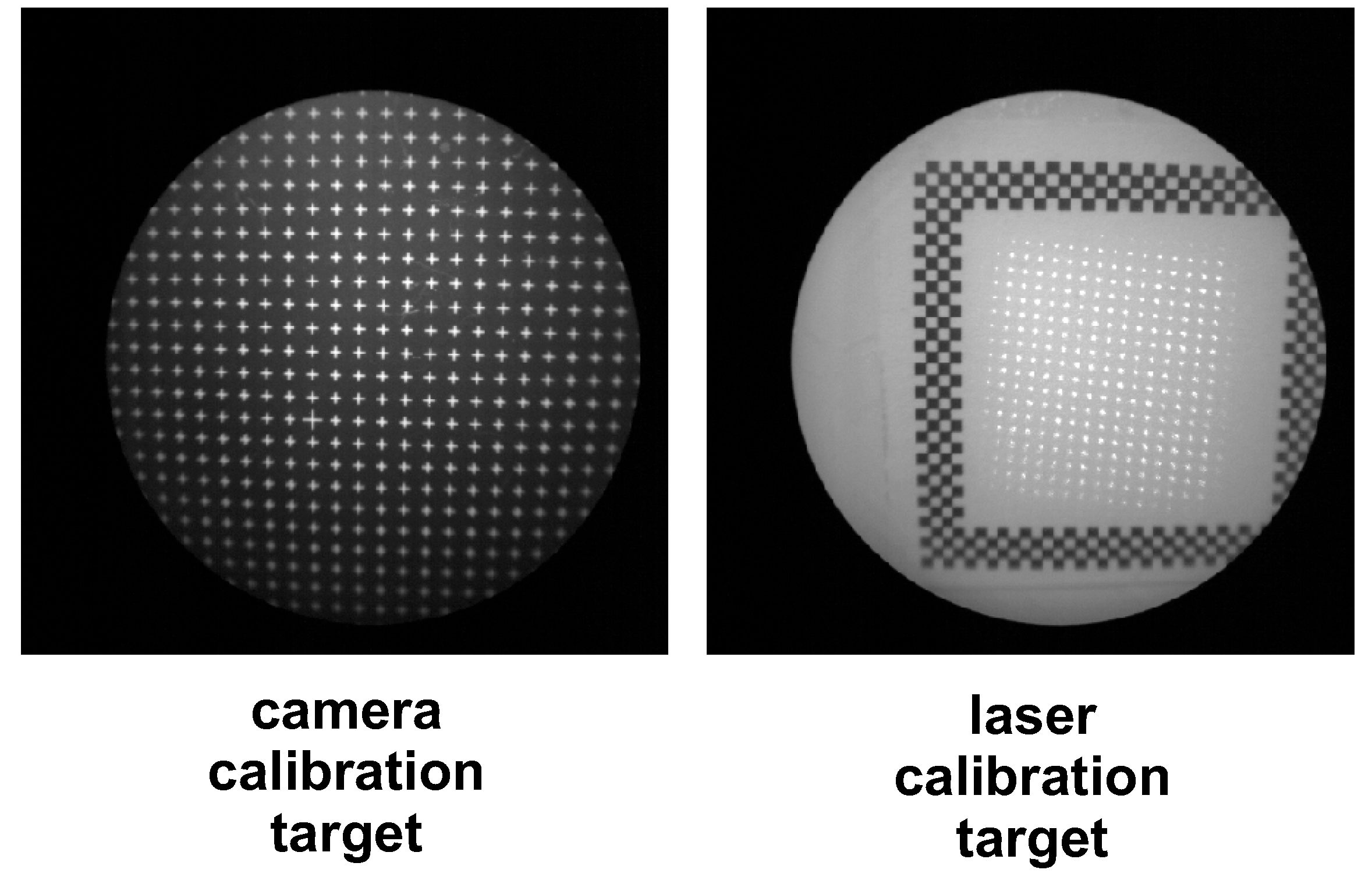
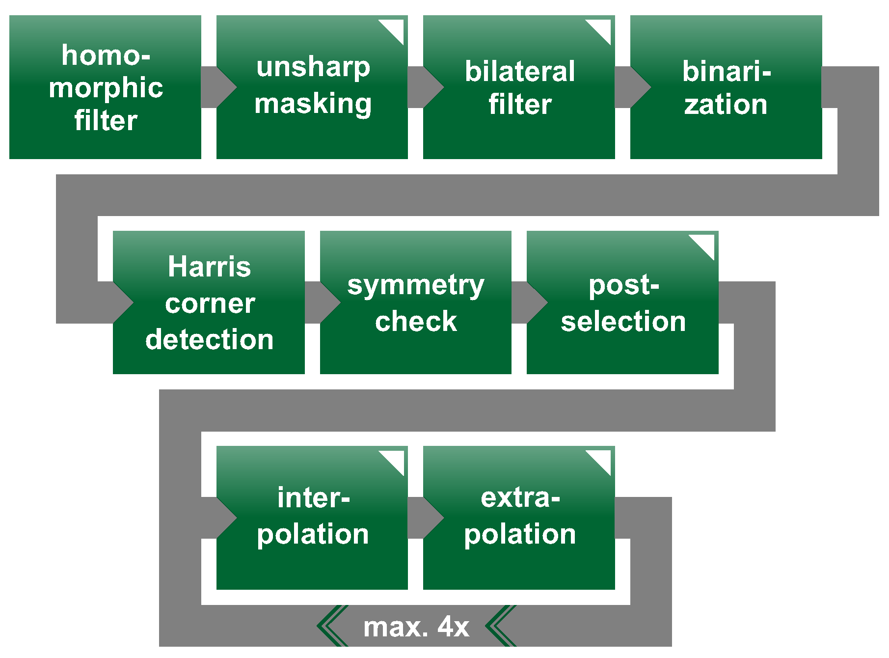
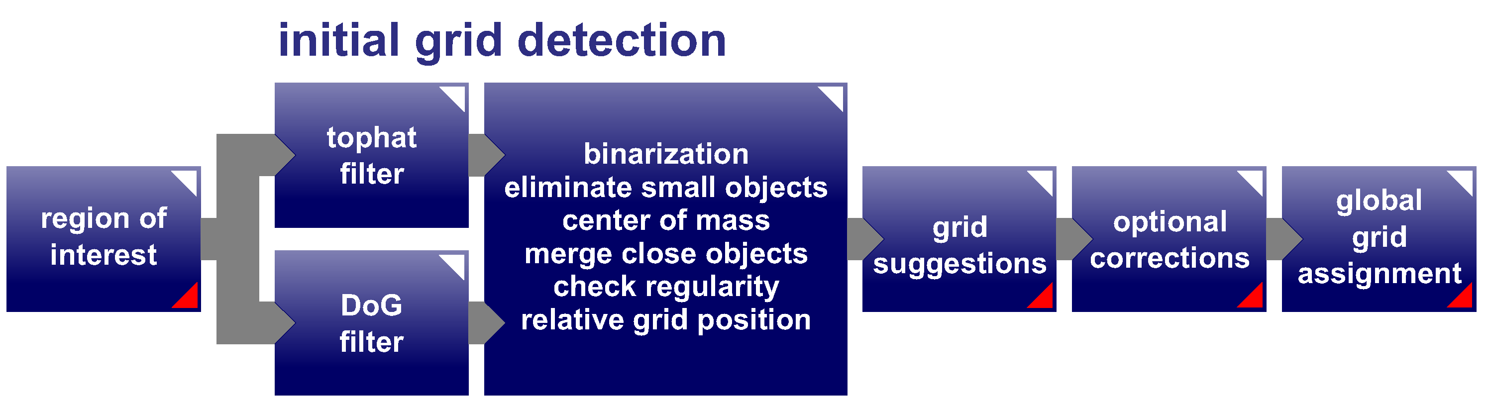
2.2.2. Challenges and Automation of Calibration Process

The quality of the laser calibration images is fairly homogeneous within one calibration series but highly variable between different experimental settings depending on the camera, the laser and the surrounding lighting. In order to apply the calibration algorithm in the clinical routine, the procedure must be highly flexible and robust.

Building on existing work, the corner detection algorithm as described in [20] is extended by several pre- and post-processing steps. A simplified flowchart of the presented algorithm is shown in Figure 9. An adaptive pre-processing algorithm allows flexible compensation of fluctuations in the initial quality of the calibration images and therefore provides constant conditions for the following detection. Previous implementations already employed a homomorphic filter to equalize the brightness distribution throughout the image and increase the contrast. In addition to that, the calibration images are now sharpened by the use of “unsharp masking” [27] and the naturally resulting increase of noise is compensated for by a bilateral filter [28], which preserves the relevant edges and corners of the checkerboard pattern. As before, a dynamic threshold for binarization is then determined using Otsu’s method [29] and the detected corner points are checked for symmetry by the method of Wang et al. [30].

In our work, only the inner corners of the checkerboard are used, since they are more reliable for the determination of the vanishing lines, which are essential for the 3D reconstruction. In the previous algorithm, the outer edges of the checkerboard had to be removed manually. Now, a post-selection step that only allows corner points with a surrounding black-white-ratio between 38–62% replaces this dispensable interaction step. Additionally, we apply an iterative procedure interpolating and extrapolating along the axes of the previously established grid based on the average grid distance.

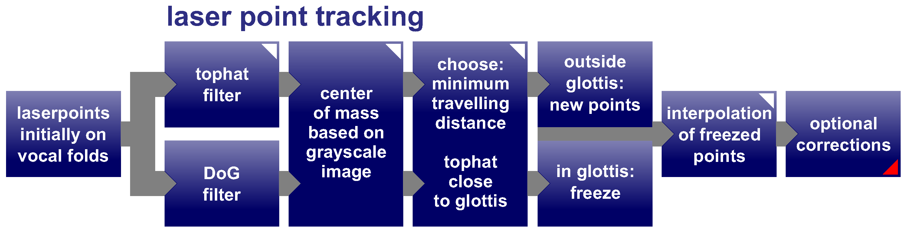
2.2.3. Challenges and Automation of Laser Point Detection

Until now [21], all relevant laser points in the initial frame had to be selected individually and the relative position with respect to its next neighbors had to be registered in a subsequent step. This procedure is very time-consuming and hardly effective. Now, we developed a semi-automatic approach to determine the laser points in the initial frame and its assignment to the respective grid positions. A flowchart of the presented algorithm is shown in Figure 10. Based on a region of interest that can be chosen by the user, the algorithm provides two different methods and suggests six different initial grids. The first method as already used in the previous tracking algorithm [21], applies a top-hat filter, which compensates for uneven illumination of the darker background in the case of bright features. The second method is based on the “Difference of Gaussians” (DoG-filter) [31]. By the subtraction of a blurred version (Gaussian filter) of the image from a less blurred version, distinct features like the laser points are enhanced in the resulting difference image. In both cases, the binarization of the images is calculated with a dynamical threshold using again Otsu’s method [29]. Small objects below average are discarded since they likely represent reflections on the mucosal vocal fold tissue. The center of mass is determined on the remaining objects and very close points are merged. In a post-selection step, the detected points are checked for regularity using triangulation. All neighboring laser points are linked by triangles and points with strongly deviating angles are eliminated. The relative grid position of each laser point is automatically concluded from the geometrical orientation to its neighbors as described by [32]. Potentially required corrections in the laser point detection (adding, moving, deleting laser points) and the grid alignment can be done manually, which is supported by a graphical user interface. However, the global grid position, which is crucial to correctly assign the corresponding homography from the calibration procedure to every individual laser point, still has to be determined by an experienced operator. This inherent difficulty of the reconstruction algorithm will be addressed in detail in Section 4.

The major challenge in tracking the laser points from frame to frame is the disappearing and reappearing of the points, which occurs only partly periodical. On the one hand, the disappearing results from the opening and closing of the glottis. The laser points within the glottis hit the tissue surface considerably deeper than the vocal folds in the subglottal area and are therefore typically not visible in the recordings. The laser points then reappear during the closing process, in which case the reassignment to the correct grid position must be guaranteed. Earlier versions of the tracking algorithm already “freezed” the laser points that lie within the glottis and suspended the tracking. However, the corresponding “unfreeze” action, when the points reappear and lie outside the glottis contour, had to be initiated manually. In addition to that, a combination with suboptimal glottis contours frequently led to a “flight” of the laser points from the glottis contour due to the gradual grayscale distribution at the vocal fold edge.

On the other hand, laser points may also be overlapped by reflections on the mucosal surface of the vocal folds. In this case, the tracking algorithm repeatedly followed the typically brighter reflections instead of the laser points if not prevented by the operator. An improved and robust tracking algorithm, which is equally efficient around the glottis and in case of reflections, requires less interaction from the user and makes the reconstruction process more effective.

Analog to the initial laser grid detection, the tracking is now also based on the top-hat filter and the DoG-filter. The corresponding flowchart is given in Figure 11. Depending on the distance from the glottis contour, the travelling distance of a laser point between two subsequent frames is restricted. Naturally, the laser points close (i.e., less than half the mean grid distance) to the glottis contour display the largest moving amplitudes. Beyond that, the algorithm gives preference to the tracking results with the smaller travelling distance. This approach successfully avoids the above mentioned “point flight”. As soon as the laser points disappear in the glottis contour, the tracking is no longer completely suspended. Instead, the points are flexibly anchored between the surrounding valid laser points outside the glottis contour. The algorithm continues to search around these anchors and tracks the reappearing points automatically. In addition to that, the detection of the subpixel position of each laser point is further refined. Previous versions calculated the center of mass on the binarized images, whereas we now utilize the original grayscale values to account for the Gaussian intensity distribution of each point.

In order to avoid any dependence on the regularity of the high-speed recordings and be able to process frequency-variable signals as well, we omitted any assumptions on periodically reappearing effects. The graphical user interface allows visually checking each frame separately and taking corrective actions if required.

3. Results and Discussion

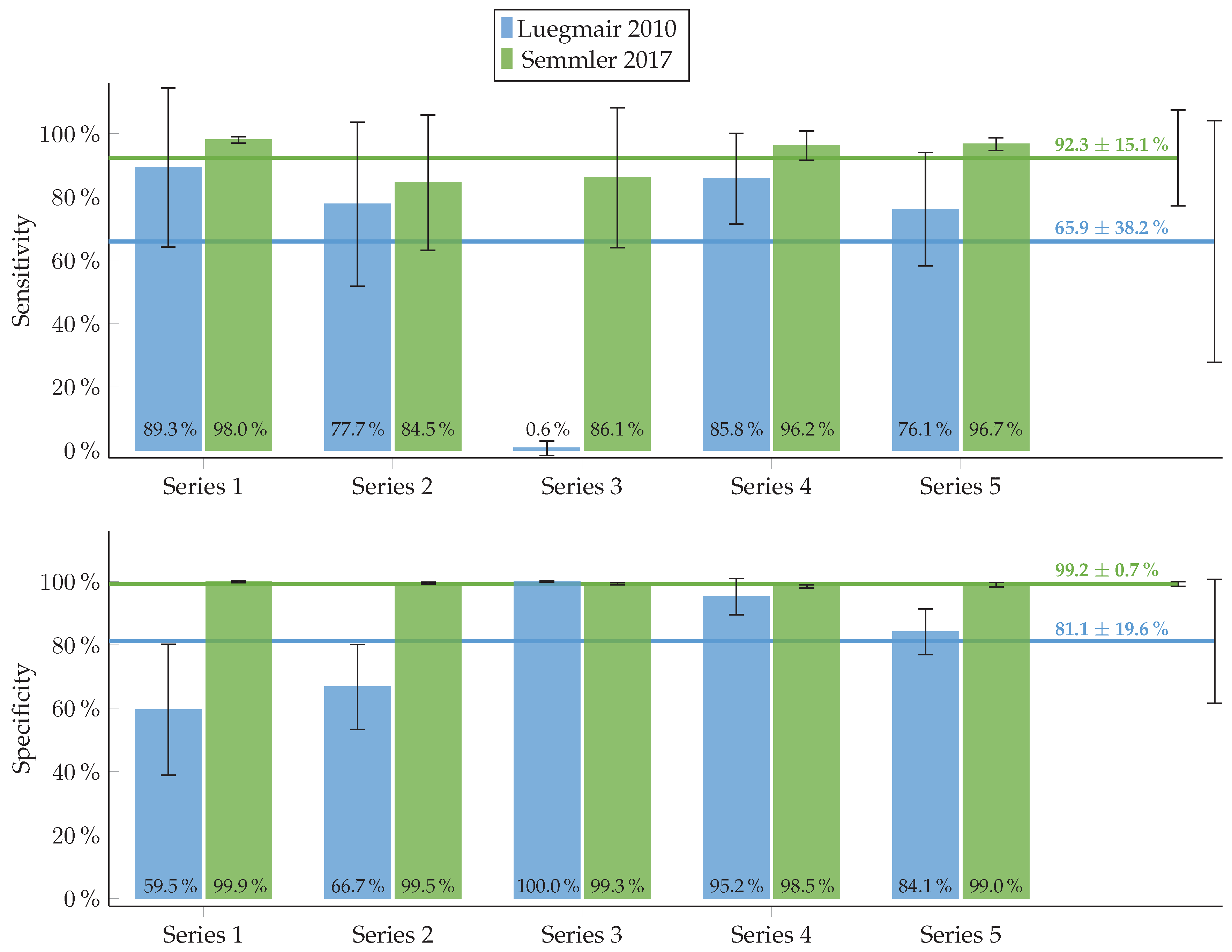
3.1. Evaluation of Automated Calibration Algorithm

In order to assess the achieved improvement of the automated calibration algorithm, we process the laser calibration images of five different series obtained from different cameras and laser projection units with 15 images each. By the use of binary classifiers, the detection results on the checkerboard pattern are categorized for each frame according to the following

Table 1. Confusion matrix for evaluation of automated calibration algorithm.

	Inner Corners of Checkerboard	Outer Corners of Checkerboard
Detected by algorithm	True positive (TP)	False positive (FP)
Not detected by algorithm	False negative (FN)	True negative (TN)

.

The sensitivity $TPR$

$$TPR=\frac{TP}{TP+FN}$$

(3)

is a measure for the success of the detection, while the success of the post-selection is quantified by the specificity $TNR$

$$TNR=\frac{TN}{TN+FP}.$$

(4)

In Figure 12, the results of the present algorithm (green) are compared to the previous calibration procedure by [20] (blue). These measures are calculated for each frame separately and then averaged over all images in each series. The vertical error bars indicate the corresponding standard deviations. The sensitivity (top) and the specificity (bottom) are significantly improved by the new pre- and post-processing steps. Please note that sensitivity and specificity have to be considered in combination with each other. The specificity of $100\%$ in Series 3 suggests a successful calibration process, but arises from the fact that the previous algorithm barely detected any corners at all as indicated by $0.6\%$ sensitivity in the same series.

The mean values in the upper right corners of Figure 12 are derived from averaging all frames of all series. The improvement in sensitivity is $40.1\%$ and in specificity $22.3\%$. Statistical analysis using IBM SPSS Statistics v21 (i.e., pairwise comparison of calibration frames over all series, applying Wilcoxon Rank Test - data was not normally distributed) showed a statistically highly significant improvement (p = 0.000) between the methods of Luegmair [20] and Semmler [22] for both measures. In addition to that, the standard deviation is considerably decreased from $38.2\%$ to $15.1\%$ for the sensitivity, which is owed to the extended pre-processing. The remarkable decrease from $19.6\%$ to $0.7\%$ in the standard deviation of the specificity arises from the newly introduced post-selection steps. This indicates a reduced dependence on the quality of the calibration images. In conclusion, these results demonstrate that the new calibration algorithm is effective and robust.

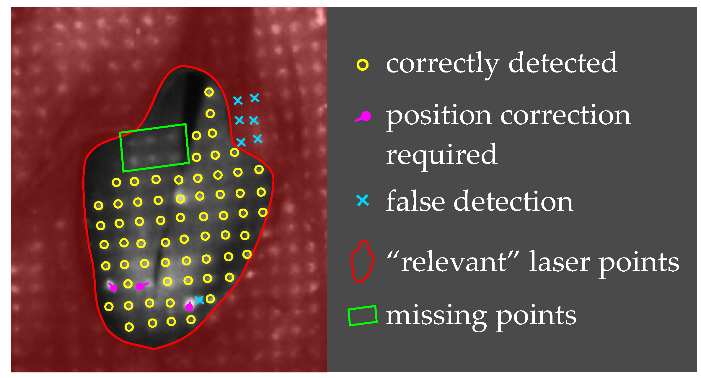
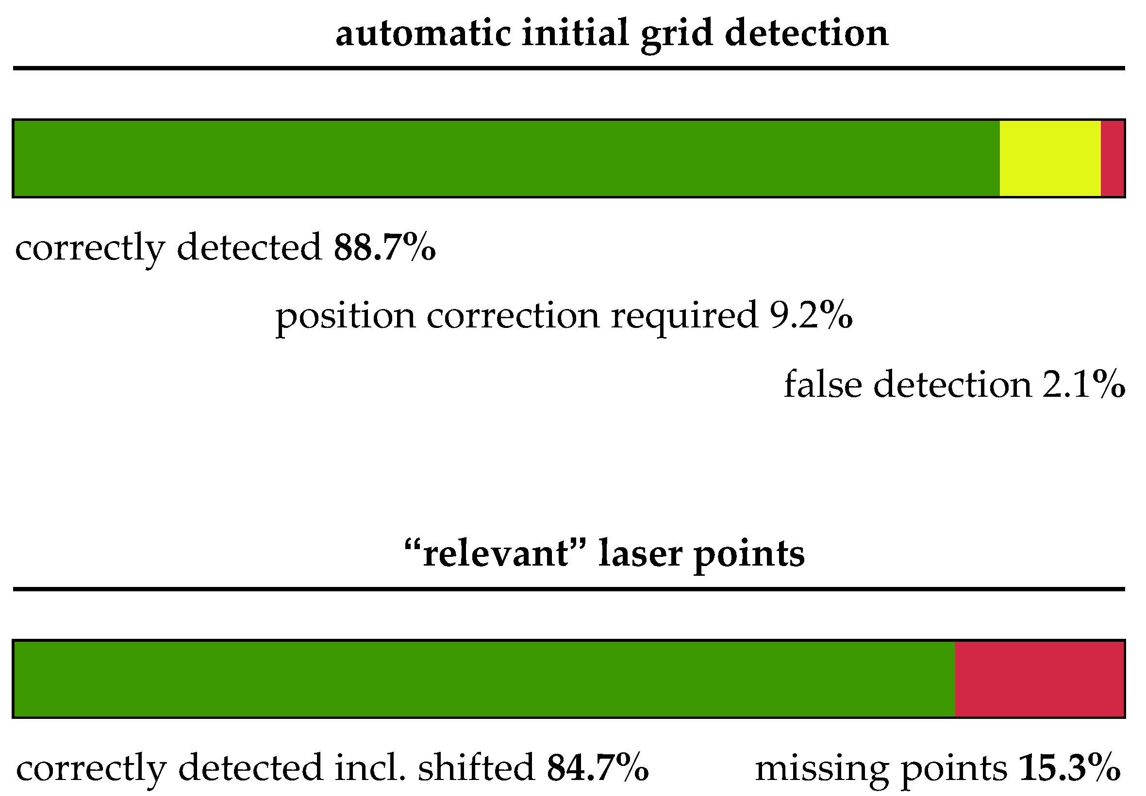
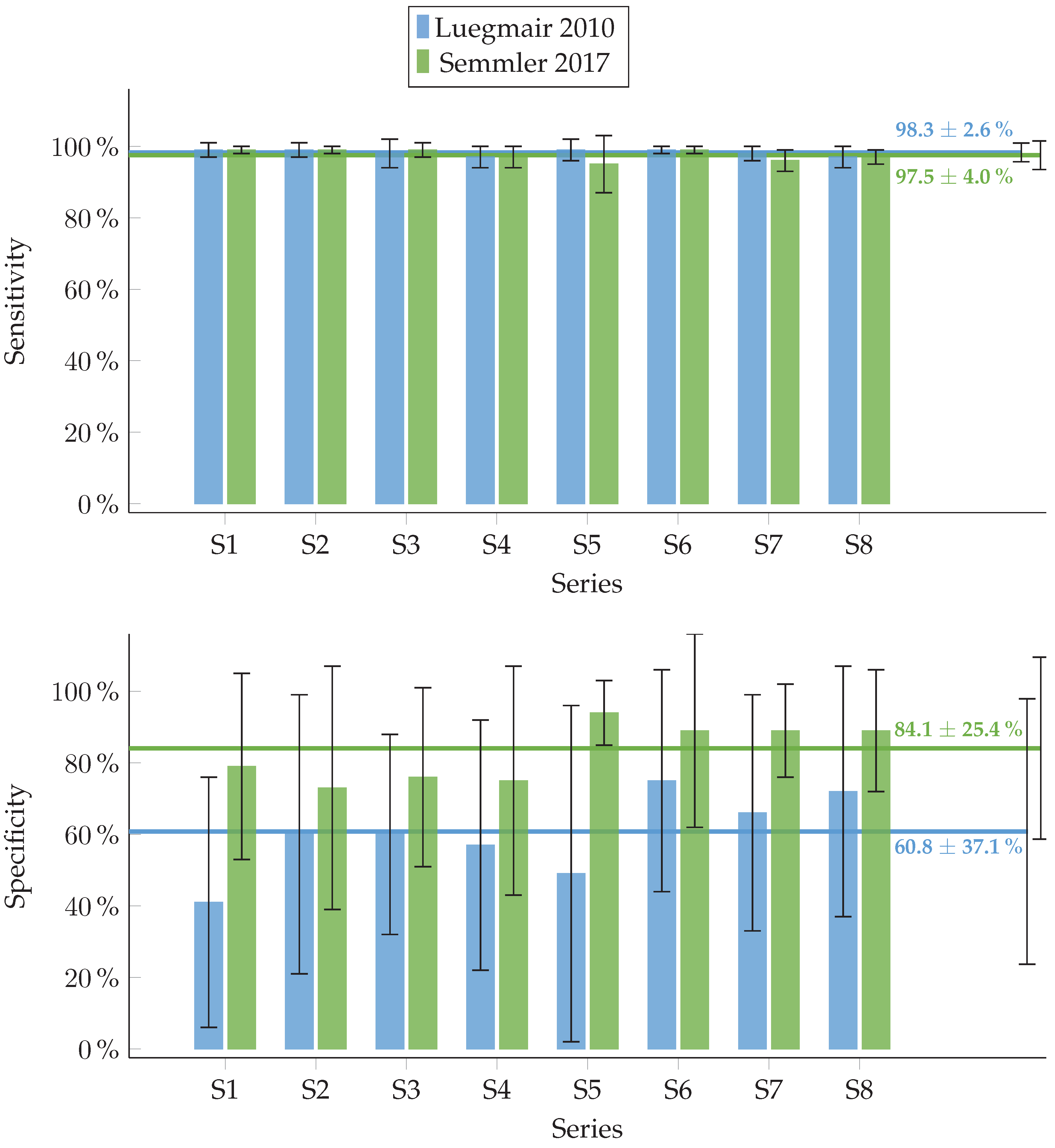
3.2. Evaluation of Automated Laser Point Detection Algorithm

For a quantification of the accomplished advances in the laser point detection algorithm, we process exemplary high-speed video recordings of eight test subjects (four females and four males recorded at 4 kHz). The initial grid detection and the tracking algorithm are assessed separately with regard to their detection success and the resulting detection duration.

The initial grid detection is performed on the first frame displaying the glottis in a closed state. A sample frame including all possible detection results and the classifying nomenclature are shown in Figure 13. The algorithm is supposed to detect all “relevant” laser points (as indicated by the red enclosing line in Figure 13), i.e., the laser points on the vocal folds but not the ones on the epiglottis, the arytenoid cartilages and the pharynx walls.

On average, the best suggestion of the automatic initial grid detection provides 88.7% correctly detected laser points (yellow circles in Figure 13). 9.2% of the initially suggested grid points require an adjustment in their position (pink dots in Figure 13) and only 2.1% of the detected points prove to be erroneous, i.e., specular reflections instead of laser points or not relevant (light blue crosses in Figure 13). The combined number of the initially correct and adjusted laser points constitutes a portion of 84.7% of the desired, objective laser grid on the vocal folds. The remaining 15.3% of the points have to be added manually by the means of the graphical user interface (points within green area in Figure 13). The corresponding quantitative results are shown in Figure 14.

The laser points from the first frame are then tracked in all frames over the following five oscillation cycles, which corresponds to 61 – 116 frames in our example files depending on the phonation frequency. The assessment of the tracking algorithm follows the procedure in Section 3.1. The detection results for each frame are categorized according to

Table 2. Confusion matrix for evaluation of the automated laser point tracking algorithm.

	Discernible	Indiscernible
	Laser Points	Laser Points
Detected by algorithm (not freezed)	True positive (TP)	False positive (FP)
Not detected by algorithm (freezed)	False negative (FN)	True negative (TN)

.

The sensitivity $TPR$ as given in (3) is a measure for the correct tracking and the automatic “unfreeze” action, while the specificity $TNR$ as given in (4) quantifies the success of the automatic “freeze” action. The results are depicted in Figure 15, allowing a direct comparison between the present (green) and the previous algorithm (blue) [20]. As before, the sensitivity (top) and specificity (bottom) are calculated for each frame separately and then averaged over all frames within each series. The total average values (on the right) are determined over all frames of all series. The vertical error bars indicate the corresponding standard deviations. The sensitivity of the tracking algorithm has already been very high in the previous implementation and is now slightly decreased within the range of the standard deviation by 0.8%. The specificity, however, is significantly increased by 38.3%. Statistical analysis using IBM SPSS Statistics v21 (i.e., pairwise comparison of video frames over all series, applying Wilcoxon Rank Test - data was not normally distributed) showed a statistically highly significant improvement (p = 0.000) between the methods of Luegmair [20] and Semmler [22] for both measures. As before, the standard deviation of the specificity is reduced from 37.1% to 25.4%, which indicates a decreased dependence on the quality of the high-speed footage.

With regard to an effective application in the clinical routine, we further evaluated the duration required to process the high-speed video recordings. Figure 16 shows the respective processing durations of the previous detection algorithm [20] (blue) and the present implementation (green). Please note, that the initial grid detection by [20] is not automated in any way, but had to be done completely manually. The automation of the initial grid detection saves 41.1% of the required time and the advances in the tracking algorithm save 42.2% in the tracking duration. Over all, the duration could be reduced from 46.5 to 27.0 min, which corresponds to a reduction of 41.9%. In summary, it can be concluded that the advances in the laser point detection algorithm increased the robustness and effectiveness while decreasing the total duration. Please, note that the evaluation of the processing duration has to be considered an estimation rather than a measurement. An extensive analysis of algorithms including a detailed run-time analysis will not be expedient until the automation is completed and the clinical application is imminent.

4. Outlook

The global grid assignment for which we need to identify the absolute position of a laser point in the grid, presents a considerable challenge during the course of reconstruction. In contrast to ex vivo experiments where a highly controlled setting can ensure a sufficient visibility of grid edges and corners, in vivo recordings suffer from the limited space in the pharynx. Shadows from superior structures and distortion of the laser points on the extreme curvature of the epiglottis and the lateral pharynx walls affect the laser grid especially in the peripheral areas (see Figure 17).

The current standard approach to face this challenge requires an experienced operator thoroughly watching the complete footage in order to identify significant edges and corners which is very time consuming and still prone to errors. Due to the geometry of the experimental set-up, mistakes in the global assignment of the grid produce a dramatic effect on the results. A mistaken offset of only one column in the assignment results in a shift of the entire reconstructed structure of about $6.4\mathrm{mm}$ along the vertical axis.

In order to compensate for this shortcoming, we suggest deviating from the conventional, regular grid as shown in Figure 18 (on the left) and using a spatially irregular laser grid instead. By the use of diffractive optical elements and liquid crystal-based spatial light modulators, it is possible to imprint any desired pattern on the spatial distribution of the laser projection. A centered cross hair in the regular grid as depicted in Figure 18 (middle) would facilitate the global grid assignment in the absence of the outer edges and corners. However, the cross hair itself cannot be relied on for the 3D reconstruction. Another conceivable approach might be a random pattern of laser points as in Figure 18 (on the right), where each subset of points displays a unique spacing towards its neighbors. This could however be impaired by a distortion of the relative distances due to the curvature of the vocal folds.

Nevertheless, we strongly believe that the use of an irregular laser projection will allow for further automation of the detection algorithms and significantly reduce its proneness to errors. This improvement will greatly facilitate the analysis of the preclinical trials, which we have planned to determine the added value by the 3D-laserendoscopy for future patients.

5. Conclusions

In respect of the clinical premises demanding highest standards, we achieved significant progress concerning the safety and the effectiveness of 3D vocal fold reconstruction from 2D high-speed recordings by the use of laserendoscopy.

We found an acceptable compromise between the mandatory safety during laser light exposure and sufficient visibility conditions for automated image processing. Following the guidelines of the ICNIRP, we developed a measuring device and a corresponding exposure limit that is officially authorized by the ethics committee. The visibility issue is successfully improved as demonstrated by the enhanced automation results. This indicates that the measuring device is now meeting the variable dimensions occurring in the daily routine of clinical application.

In addition to an improved starting situation due to optimal brightness and contrast, the effectiveness of the reconstruction procedure could be further raised by an increased degree of automation in the calibration and reconstruction procedure. The number of interactions required from the operator and the overall reconstruction duration could be reduced. The options for potential corrections are conveniently integrated in a graphical user interface.

Nevertheless, further improvements on the reconstruction procedure and the global grid registration are necessary in order to achieve a real time analysis. Assuming these changes, the clinical application of the 3D reconstruction from high-speed recordings with a laser projection is within reach. 3D parameters that incorporate the information on an additional dimension compared to established 2D parameters from kymography and phonovibrograms, will deliver an objective and comprehensive measure to quantify therapeutic effects on the vocal fold dynamics. Providing the complete superior vocal fold surface, the laserendoscopy will be a valuable tool for an evidence-based diagnostic procedure.

References

1. Ruben, R.J. Redefining the survival of the fittest: Communication disorders in the 21st century. Laryngoscope 2000, 110, 241–245. [Google Scholar] [CrossRef] [PubMed]
2. Stevens, K.N. Acoustic Phonetics; MIT Press: Cambridge, MA, USA, 1998. [Google Scholar]
3. Patel, R.R.; Dubrovskiy, D.; Döllinger, M. Measurement of Glottal Cycle Characteristics Between Children and Adults: Physiological Variations. J. Voice 2014, 28, 476–486. [Google Scholar] [CrossRef] [PubMed]
4. Bohr, C.; Kräck, A.; Dubrovskiy, D.; Eysholdt, U.; Svec, J.; Psychogios, G.; Ziethe, A.; Döllinger, M. Spatiotemporal Analysis of High-Speed Videolaryngoscopic Imaging of Organic Pathologies in Males. J. Speech Lang. Hear. Res. 2014, 57, 1148–1161. [Google Scholar] [CrossRef] [PubMed]
5. Echternach, M.; Döllinger, M.; Sundberg, J.; Traser, L.; Richter, B. Vocal fold vibrations at high soprano fundamental frequencies. J. Acoust. Soc. Am. 2013, 133, EL82–EL87. [Google Scholar] [CrossRef] [PubMed]
6. Petermann, S.; Kiesburges, S.; Ziethe, A.; Schützenberger, A.; Döllinger, M. Evaluation of Analytical Modeling Functions for the Phonation Onset Process. Comput. Math. Methods Med. 2016, 2016, 8469139. [Google Scholar] [CrossRef] [PubMed]
7. Schützenberger, A.; Kunduk, M.; Döllinger, M.; Alexiou, C.; Dubrovskiy, D.; Semmler, M.; Seger, A.; Bohr, C. Laryngeal High-Speed Videoendoscopy: Sensitivity of Objective Parameters towards Recording Frame Rate. BioMed Res. Int. 2016, 2016, 4575437. [Google Scholar] [CrossRef] [PubMed]
8. Svec, J.G.; Schutte, H.K. Videokymography: High-speed line scanning of vocal fold vibration. J. Voice 1996, 10, 201–205. [Google Scholar] [CrossRef]
9. Lohscheller, J.; Eysholdt, U. Phonovibrogram Visualization of Entire Vocal Fold Dynamics. Laryngoscope 2008, 118, 753–758. [Google Scholar] [CrossRef] [PubMed]
10. Döllinger, M.; Berry, D.A. Computation of the three-dimensional medial surface dynamics of the vocal folds. J. Biomech. 2006, 39, 369–374. [Google Scholar] [CrossRef] [PubMed]
11. Döllinger, M.; Berry, D.A.; Kniesburges, S. Dynamic vocal fold parameters with changing adduction in ex-vivo hemilarynx experiments. J. Acoust. Soc. Am. 2016, 139, 2372. [Google Scholar] [CrossRef] [PubMed]
12. Döllinger, M.; Berry, D.A. Visualization and Quantification of the Medial Surface Dynamics of an Excised Human Vocal Fold During Phonation. J. Voice 2006, 20, 401–413. [Google Scholar] [CrossRef] [PubMed]
13. Sommer, D.E.; Tokuda, I.T.; Peterson, S.D.; Sakakibara, K.I.; Imagawa, H.; Yamauchi, A.; Nito, T.; Yamasoba, T.; Tayama, N. Estimation of inferior-superior vocal fold kinematics from high-speed stereo endoscopic data in vivo. J. Acoust. Soc. Am. 2014, 136, 3290–3300. [Google Scholar] [CrossRef] [PubMed]
14. Hoppe, U.; Rosanowski, F.; Döllinger, M.; Lohscheller, J.; Schuster, M.; Eysholdt, U. Glissando: Laryngeal motorics and acoustics. J. Voice 2003, 17, 370–376. [Google Scholar] [CrossRef]
15. Larsson, H.; Hertegard, S. Calibration of high-speed imaging by laser triangulation. Logop. Phoniatr. Vocol. 2004, 29, 154–161. [Google Scholar] [CrossRef] [PubMed]
16. Patel, R.R.; Donohue, K.D.; Johnson, W.C.; Archer, S.M. Laser projection imaging for measurement of pediatric voice. Laryngoscope 2011, 121, 2411–2417. [Google Scholar] [CrossRef] [PubMed]
17. George, N.A.; de Mul, F.F.M.; Qiu, Q.; Rakhorst, G.; Schutte, H.K. Depth-kymography: High-speed calibrated 3D imaging of human vocal fold vibration dynamics. Phys. Med. Biol. 2008, 53, 2667–2675. [Google Scholar] [CrossRef] [PubMed]
18. Wurzbacher, T.; Voigt, I.; Schwarz, R.; Döllinger, M.; Hoppe, U.; Penne, J.; Eysholdt, U.; Lohscheller, J. Calibration of laryngeal endoscopic high-speed image sequences by an automated detection of parallel laser line projections. Med. Image Anal. 2008, 12, 300–317. [Google Scholar] [CrossRef] [PubMed]
19. Patel, R.; Donohue, K.; Lau, D.; Unnikrishnan, H. In vivo measurement of pediatric vocal fold motion using structured light laser projection. J. Voice 2013, 27, 463–472. [Google Scholar] [CrossRef] [PubMed]
20. Luegmair, G.; Kniesburges, S.; Zimmermann, M.; Sutor, A.; Eysholdt, U.; Döllinger, M. Optical reconstruction of high-speed surface dynamics in an uncontrollable environment. IEEE Trans. Med. Imaging 2010, 29, 1979–1991. [Google Scholar] [CrossRef] [PubMed]
21. Luegmair, G.; Mehta, D.D.; Kobler, J.B.; Döllinger, M. Three-Dimensional Optical Reconstruction of Vocal Fold Kinematics Using High-Speed Video With a Laser Projection System. IEEE Trans. Med. Imaging 2015, 34, 2572–2582. [Google Scholar] [CrossRef] [PubMed]
22. Semmler, M.; Kniesburges, S.; Birk, V.; Ziethe, A.; Patel, R.; Döllinger, M. 3D Reconstruction of Human Laryngeal Dynamics Based on Endoscopic High-Speed Recordings. IEEE Trans. Med. Imaging 2016, 35, 1615–1624. [Google Scholar] [CrossRef] [PubMed]
23. International Commission on Non-Ionizing Radiation Protection. Guidelines on Limits of Exposure to Laser Radiation of Wavelengths between 180 nm and 1000 μm. Health Phys. 2013, 105, 271–295. [Google Scholar]
24. World Medical Association. WMA Declaration of Helsinki: Ethical principles for medical research involving human subjects. JAMA 2013, 310, 2191–2194. [Google Scholar]
25. Hartley, R.; Zisserman, A. Multiple View Geometry in Computer Vision; Cambridge University Press: Cambridge, UK, 2000. [Google Scholar]
26. Döllinger, M.; Dubrovskiy, D.; Patel, R. Spatiotemporal analysis of vocal fold vibrations between children and adults. Laryngoscope 2012, 122, 2511–2518. [Google Scholar] [CrossRef] [PubMed]
27. Polesel, A.; Ramponi, G.; Mathews, V.J. Image enhancement via adaptive unsharp masking. IEEE Trans. Image Process. 2000, 9, 505–510. [Google Scholar] [CrossRef] [PubMed]
28. Chaudhury, K.N.; Dabhade, S.D. Fast and Provably Accurate Bilateral Filtering. IEEE Trans. Image Process. 2016, 25, 2519–2528. [Google Scholar] [CrossRef] [PubMed]
29. Otsu, N. A Threshold Selection Method from Gray-Level Histograms. IEEE Trans. Syst. Man Cybern. 1979, 9, 62–66. [Google Scholar] [CrossRef]
30. Wang, Z.; Wang, Z.; Wu, Y. Recognition of corners of planar pattern image. In Proceedings of the 8th World Congress on Intelligent Control and Automation, Jinan, China, 7–9 July 2010; pp. 6342–6346. [Google Scholar]
31. Lindeberg, T. Image Matching Using Generalized Scale-Space Interest Points. J. Math. Imaging Vis. 2015, 52, 3–36. [Google Scholar] [CrossRef]
32. Luegmair, G. 3D Reconstruction Of Vocal Fold Surface Dynamics in Functional Dysphonia. Ph.D. Thesis, Friedrich-Alexander-Universität Erlangen Nürnberg, Erlangen, Germany, 2014. [Google Scholar]
Figure 1. Schematic overview of the three-dimensional vocal fold vibration during phonation: The vertical displacement amplitudes are in the same magnitude as the mainly and commonly analyzed lateral displacement amplitudes [11].
Applsci 07 00600 g001
Figure 2. Overview of the experimental measuring device. The imaging unit comprises a rigid 70 -laryngoscope, a zoom coupler and a high-speed camera. A frequency-doubled Nd:YAG laser source is connected to the laser projection unit via a glass fiber. Different perspectives on the tip of the miniaturized endoscopic laser projection unit are provided on the left.
Applsci 07 00600 g002
Figure 3. Schematic of the optical set-up within the laser projection unit (LPU): The diffractive optical element is a customized, binary phase mask generating a laser grid of 31 × 31 points. All optical elements have an anti-reflective coating for 532 nm.
Applsci 07 00600 g003
Figure 4. Gaussian intensity distribution of laser beams in the grid at a working distance of 65 mm: cross-sectional measurement of individual laser spots and determination of 1 / e 2 radius at 400 μ m.
Applsci 07 00600 g004
Figure 5. Projection of regular laser grid (31 × 31 individual spots) at a working distance of 50 , 65 and 80 mm (from left to right) with a uniformity of 10% regarding the size and intensity of each point.
Applsci 07 00600 g005
Figure 6. Beam caustic comparison: average diameter of an individual laser point in the grid with respect to the position beneath the tip of the laserendoscope.
Applsci 07 00600 g006
Figure 7. Flowchart of the calibration and reconstruction process. White corners indicate new processing steps.
Applsci 07 00600 g007
Figure 8. Calibration targets: white crosses on black background for camera calibration and a checkerboard frame for laser calibration.
Applsci 07 00600 g008
Figure 9. Flowchart of the calibration process. White corners indicate new processing steps.
Applsci 07 00600 g009
Figure 10. Flowchart of the initial grid detection. White corners indicate new processing steps and red corners indicate a necessary or optional user interaction.
Applsci 07 00600 g010
Figure 11. Flowchart of the laser point tracking. White corners indicate new processing steps and red corners indicate a necessary or optional user interaction.
Applsci 07 00600 g011
Figure 12. Evaluation of the automated calibration algorithm compared to its previous version by [20] including the sensitivity (top) and the specificity (bottom). The depicted bars represent the average value for each series while the vertical error bars indicate the standard deviation within each series. The horizontal lines represent the average value over all frames of all series and the error bars indicate the corresponding standard deviation.
Applsci 07 00600 g012
Figure 13. Classification scheme for the evaluation of initial grid detection algorithm.
Applsci 07 00600 g013
Figure 14. Evaluation of the automated initial grid detection algorithm including an analysis of the initially suggested laser grid (top) and the success with respect to the desired, objective grid (bottom).
Applsci 07 00600 g014
Figure 15. Evaluation of the automated laser point tracking algorithm compared to its previous version by [20] including the sensitivity (top) and the specificity (bottom). The depicted bars represent the average value for each series while the vertical error bars indicate the standard deviation within each series. The horizontal lines represent the average value over all frames of all series and the error bars indicate the corresponding standard deviation.
Applsci 07 00600 g015
Figure 16. Evaluation of total duration of the laser point detection algorithm compared to its previous implementation by [20] subdivided in the initial grid detection and the tracking algorithm.
Applsci 07 00600 g016
Figure 17. Uncontrollable conditions for global grid assignment in in vivo recordings due to shadows or distortions of the grid points on pharynx tissue.
Applsci 07 00600 g017
Figure 18. Different designs for laser projection grid: regularly structured grid (left), regularly structured grid with cross hair (middle), randomly structured grid (right).
Applsci 07 00600 g018