
Member Discrete Element Method for Static and Dynamic Responses Analysis of Steel Frames with Semi-Rigid Joints

1
State Key Laboratory for Geomechanics & Deep Underground Engineering, China University of Mining and Technology, Xuzhou 221116, China
2
Key Laboratory of Concrete and Pre-Stressed Concrete Structures of the Ministry of Education, Southeast University, Nanjing 210018, China
*
Author to whom correspondence should be addressed.
Appl. Sci. 2017, 7(7), 714; https://doi.org/10.3390/app7070714
Submission received: 27 May 2017
/
Revised: 6 July 2017
/
Accepted: 7 July 2017
/
Published: 11 July 2017
(This article belongs to the Special Issue Development and Application of Nonlinear Dissipative Device in Structural Vibration Control)
Abstract
:Featured Application
The MDEM can naturally deal with strong nonlinearity and discontinuity. A unified computational framework is applied for static and dynamic analyses. The method is an effective tool to investigate complex behaviors of steel frames with semi-rigid connections.
Abstract
In this paper, a simple and effective numerical approach is presented on the basis of the Member Discrete Element Method (MDEM) to investigate static and dynamic responses of steel frames with semi-rigid joints. In the MDEM, structures are discretized into a set of finite rigid particles. The motion equation of each particle is solved by the central difference method and two adjacent arbitrarily particles are connected by the contact constitutive model. The above characteristics means that the MDEM is able to naturally handle structural geometric nonlinearity and fracture. Meanwhile, the computational framework of static analysis is consistent with that of dynamic analysis, except the determination of damping. A virtual spring element with two particles but without actual mass and length is used to simulate the mechanical behaviors of semi-rigid joints. The spring element is not directly involved in the calculation, but is employed only to modify the stiffness coefficients of contact elements at the semi-rigid connections. Based on the above-mentioned concept, the modified formula of the contact element stiffness with consideration of semi-rigid connections is deduced. The Richard-Abbort four-parameter model and independent hardening model are further introduced accordingly to accurately capture the nonlinearity and hysteresis performance of semi-rigid connections. Finally, the numerical approach proposed is verified by complex behaviors of steel frames with semi-rigid connections such as geometric nonlinearity, snap-through buckling, dynamic responses and fracture. The comparison of static and dynamic responses obtained using the modified MDEM and those of the published studies illustrates that the modified MDEM can simulate the mechanical behaviors of semi-rigid connections simply and directly, and can accurately effectively capture the linear and nonlinear behaviors of semi-rigid connections under static and dynamic loading. Some conclusions, as expected, are drawn that structural bearing capacity under static loading will be overestimated if semi-rigid connections are ignored; when the frequency of dynamic load applied is close to structural fundamental frequency, hysteresis damping of nonlinear semi-rigid connections can cause energy dissipation compared to rigid and linear semi-rigid connections, thus avoiding the occurrence of resonance. Additionally, fracture analysis also indicates that semi-rigid steel frames possess more anti-collapse capacity than that with rigid steel frames.
1. Introduction
Beam-to-column joints are frequently simplified to be fully rigid or pinned connections in structural analyses and designs, while real beam-to-column joints are semi-rigid connections between the two extreme cases. Compared with rigid connections, semi-rigid connections will reduce total stiffness of steel frames and make lateral displacement increase, thereby causing a second-order effect [1]. Therefore, the rigidity of a semi-rigid joint has a significant effect on the strength and displacement response of steel frames. At present, approaches for investigating mechanical behaviors of semi-rigid joints fall into three categories: experiment, mathematical model and numerical simulation. For the first two approaches, an amount of mature research has been carried out, and a variety of linear or nonlinear semi-rigid connection models were proposed [2,3,4,5,6]. Furthermore, Eurccode-3 (EC3) [7] provides the M-θ curves for some specified beam-to column joints of steel structures. Based on the M-θ curves of EC3, Keulen et al. [8] introduced the half initial secant stiffness approach to simplify the full characteristics of nonlinear connection stiffness curve into a bilinear curve in practical design, and analysis results of the two cases were in good agreement. Thus, numerical simulation methods of semi-rigid joints have increasingly attracted the attentions of numerous researchers in recent years.
The finite element method (FEM) is the most commonly used method in the numerical simulation of semi-rigid joints. Lui and Chen [9], Ho and Chen [10] considered structural geometric nonlinearity by stability functions, and analyzed nonlinearity and buckling behaviors of semi-rigid beam-to-column joints in conjunction with the geometric stiffness matrix and updated Lagrangian approach. Yau and Chan [11] presented a beam-column element with springs connected in series for geometric and material nonlinear analysis of steel frames with semi-rigid connections, as well as proposed an efficient approach to trace the equilibrium path of steel frames. Zhou and Chan [12] performed second-order analysis of steel frames with semi-rigid connections by a displacement-based finite-element approach. Chui and Chan [13,14], Sophianopoulos [15] investigated the dynamic responses of steel frames with semi-rigid joints, where a semi-rigid joint was simulated by a zero-length spring element. Li et al. [16] and Rodrigues et al. [17] presented a multi-degree of freedom spring system to represent physical models of semi-rigid connections and took semi-rigid connections as new elements. This system transferred axial forces, shearing forces as well as bending moments. All the above results are based on the conventional finite-element method. However, in the static or dynamic analyses especially for strong nonlinear and discontinuous problems, the method has some limits such as difficult modeling, plenty of unknowns, long consuming time and convergence difficulty. In order to shorten consuming time, Nguyen and Kim [18,19] proposed a numerical procedure based on the beam-column method, and performed nonlinearly elastic and inelastic time-history analysis of three-dimensional semi-rigid steel frames by using the based-displacement finite element method. Compared to SAP2000(Computers and Structures, Inc., California, CA, USA), the procedure captured the second-order effect by using only one element per member, and reduced computational time. Nevertheless, it failed to model fracture behaviors of steel frames with semi-rigid joints. Lien and Chiou [20], Yu and Zhu [21] carried out an investigation on dynamic collapse of semi-rigid steel frames using vector formed intrinsic finite-element (VFIFE) method. A zero-length spring element was employed to simulate the semi-rigid joints. However, the spring element is involved in the calculation, which makes that the method has a cumbersome calculation process and long consuming time. In addition, for discontinuous issues, this method needs to regenerate a new particle at the point where fracture occurs, causing the computation time to increase again.
Different from the aforementioned methods derived from continuum mechanics, the theoretical basis of Member Discrete Element Method (MDEM) presented by Ye team [22] according to conventional Particle Discrete Element [23] is non-continuum mechanics. In the MDEM, a member is represented by a set of finite particle rather than by continuum. The motion equation of each particle is solved by the central difference method and arbitrarily adjacent particles are connected by the contact constitutive model. The difference between the MDEM and conventional DEM lies in the establishment of the contact constitutive model. Therefore, the MDEM not only extends the application range of conventional DEM, but also inherits its advantages such as no assembly of stiffness matrix and iterative solution of motion equations, no special treatment for nonlinear issues, no re-meshing for fracture problems, and no convergence difficulty. At present, the method has been successfully applied to geometric nonlinearity [24] and nonlinear dynamic analysis [25] of member structures as well as progressive collapse simulation of reticulated shells [22]. These results show that the MDEM is a simple and effective tool to process geometrically large deformation, material nonlinearity and fracture issues. However, no report that the MDEM is adopted for static and dynamic response analysis of steel frames with semi-rigid joints exists.
A simple and effective numerical approach is proposed based on the MDEM for static and dynamic response analysis of steel frames with semi-rigid joints. Brief details of the basic theory for the MDEM are first presented including particle motion equations, particle internal forces, geometric nonlinearity modelling and fracture modeling. The semi-rigid connection is simulated by a virtual spring element, and then the modified formula of the contact element stiffness adjacent to the semi-rigid connection is derived. The nonlinear behaviors of semi-rigid connections are captured by the bilinear semi-rigid connection model and Richard-Abbort four-parameter model. Furthermore, its hysteresis behavior is traced by the independent hardening model. The correctness and accuracy of the numerical procedure proposed are verified by complex behaviors analyses of steel frames with semi-rigid connections, such as geometric nonlinearity, snap-through buckling, dynamic responses and fracture.
2. Member Discrete Element Method (MDEM)
2.1. Particle Motion Equations and Internal Forces
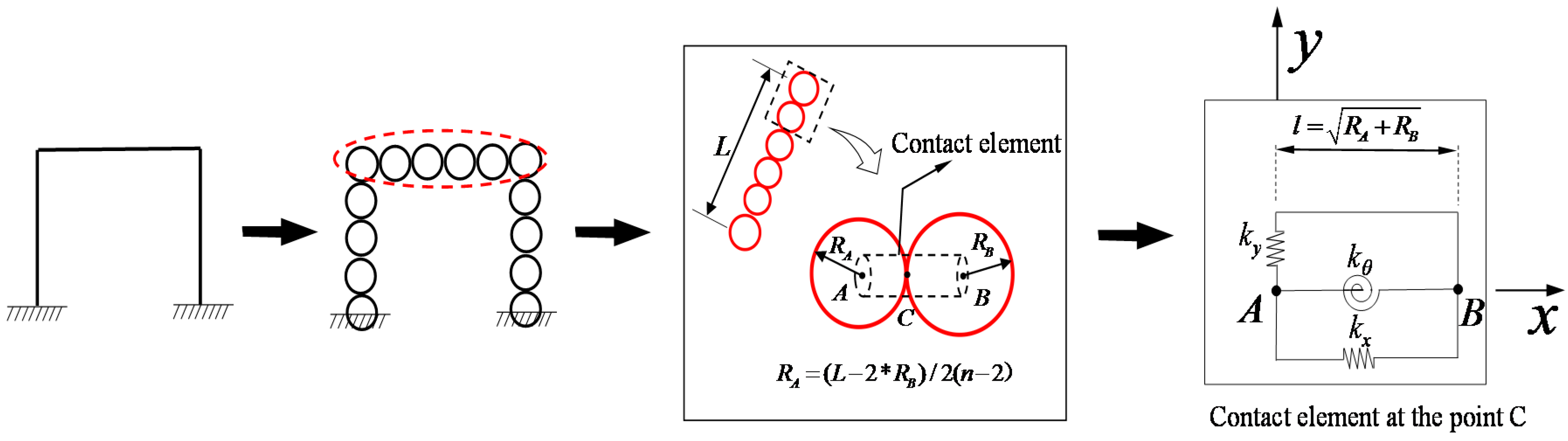
The Member Discrete Element Method (MDEM) presented by Ye team [22] discretizes a steel frame into a set of finite rigid particles, and adjacent particles (e.g., Particles A and B) are connected by the contact element (i.e., contact constitutive model), as shown in Figure 1. The criterion for the number of particles in the MDEM is consistent with that for beam elements in FEM, which is detailed in Reference [26]. The method not only overcomes the difficulties of conventional FEM in processing strong nonlinearity and discontinuity, but also eliminates the shortcomings with low precision, long consuming time and poor applicability of conventional DEM. The calculation framework of the MDEM consists of two parts: particle motion equations and particle internal forces, which is briefly elaborated below.
2.1.1. Particle Motion Equations
The motion of each particle follows the Newton’s second law at any time . If damping term is supplemented to make structures static, the motion equations for an arbitrarily particle can be expressed as
where and are the equivalent mass and moment of inertia lumped at an arbitrarily particle, respectively; and denote translational and rotational acceleration vectors in the global coordinate system, respectively; and indicate translational and rotational velocity vectors in the global coordinate system, respectively; and are internal force and moment vectors acting at an arbitrarily particle, respectively; and external force and moment vectors acting at an arbitrarily particle, respectively; and and denote translational and rotational damping matrix, respectively. Additionally, and equal and in the dynamic analyses respectively while both are virtual terms under static loading. is mass proportional damping coefficient.
If the central finite difference algorithm is employed to solve Equations (1) and (2), the translational velocity and acceleration of a particle can be approximated as
where , and are the displacements of a particle at step , and , respectively; and is a constant time increment.
Substituting Equations (3) and (4) into Equation (1) yields
Equation (5) is the formula of the translational displacements of a particle.
2.1.2. Particle Internal Forces
From the discretization procedure of a three-dimension steel frame in Figure 1, it can be found that the establishment of MDEM model is different from that of the conventional DEM model. In the MDEM, the radius of the particles at both ends () of all the members is first given, and then the radii of the particles in the members () are determined via equally dividing the remaining lengths of these members. The internal forces arising at the contact points (e.g., Point C) between connected particles (e.g., Particles A and B) need be first calculated, and then they are exerted reversely to these particles (e.g., Particles A and B), thereby acquiring internal forces of an arbitrary particle in Figure 1. The internal force and moment increment at a contact point can be obtained by contact constitutive model, which are
where and are the incremental internal force and moment of inertia arising at a contact point, respectively; and indicate translational and rotational contact stiffness coefficients, respectively; and and denote pure translational and rotational displacements of a contact point in a time step respectively, which are in the local coordinate system.
The key point of the DEM is the determination of contact stiffness coefficients (i.e., and ) in Equation (6). The coefficients are obtained mainly from experiences or experiments for the conventional DEM, while the MDEM gives the formulas of contact stiffness coefficients. Prof. Ye team [22] supplemented rotational springs into contact constitutive model (Figure 1), which make that the force state of each contact element (i.e., equivalent beam AB in Figure 1) is the same as that of the spatial beam element with three translational and three rotational degrees of freedoms in the FEM. According to the strain energy equivalent principle and simple beam theory, the formulas of contact stiffness coefficients for three-dimension member structures can be expressed as [24]
where is the distance between the two particle centers; A, E and G denote the area, elastic modulus and modulus of shearing of each member, respectively; and , and are the cross sectional moments of inertia of a member about the x, y and z axes, respectively.
2.2. MDEM for Modelling Geometric Nonlinearity
Structural geometric nonlinearity comprises rigid body motion, large rotation and large deformation. For the FEM, special treatments and complex modifications are necessary to deal with problems of this kind, such as the arc-length method and co-rotational coordinate approach [27]. However, in the MFEM, particles are assumed to be rigid, and thus rigid body motion of particles can be removed naturally in the process of solving the pure displacement of contact points using the rigid body kinematics. Furthermore, the movement of each particle is represented numerically by a time-stepping algorithm. In the algorithm, the assumption of small deformation is satisfied within each time step, which makes that large deformation and large rotation issues are naturally handled [28]. Thus, the unified procedure is employed in the MDEM for geometric linear and nonlinear problems.
2.3. MDEM for Modeling Facture Behavior
Fracture behavior possesses strong discontinuity. In the FEM, fracture is modeled by defining birth-death elements or failure elements, which may cause the non-conservation of mass and convergence difficulty [26]. Nevertheless, in the MDEM, a structure is represented by a set of finite rigid particle rather than by continuum, and each particle is in a dynamic equilibrium. Given an appropriate fracture criterion only, Fracture behavior can be simulated [22]. The fracture is macroscopically represented by the separate of two adjacent particles in Figure 1. The Bending strain is take as the fracture criteria in this study, which is denoted as
where and are the bending strain at time t and ultimate bending strain, respectively. The ultimate bending strain is set to be 0.0004 according to relative experiments and studies [29].
3. Member Discrete Element Modeling for Semi-Rigid Connections
3.1. Virtual Zero-Length Spring Element
In this study, a semi-rigid joint is simulated by a multi-degree-of-freedom spring element with two particles but without actual mass and length. The basic concept of the spring element is similar to that of References [13,18]. The moment-rotation relationship of the zero-length spring element is expressed as a diagonal tangent stiffness matrix in other numerical approaches taking the FEM as a representation. In addition, the stiffness matrix needs to be integrated with structural total stiffness matrix. However, in the MDEM, the zero-length spring element is not directly involved in the calculation, but is employed only to modify the stiffness coefficient of each contact element adjacent to the semi-rigid connection. In addition, then the modified stiffness coefficient of the contact element is directly applied in the next time step. The whole procedure is simple and effective. Furthermore, computational time of the MDEM after considering semi-rigid connections has no increase. This is not only the nature difference between the zero-length spring element of the MDEM and that of other methods, but also the advantage of the MDEM processing semi-rigid connection problem.
The MDEM model of a simple frame is displayed in Figure 2. If the joint D (i.e., particle D) is a semi-rigid connection, the processing mode of the semi-rigid connection is given in Figure 3, that is, a zero-length spring element is supplemented at the particle. The spring element contains two particles E and F with same coordinates, and its translational and rotational stiffness matrix can be expressed as
where and are the translational and rotational stiffness vectors of a zero-length spring element with respect to n axis (n = x, y, z). In addition, for a two-dimensional problem, the zero-length spring element can degrade to three degrees of freedom which is two translational degrees of freedom and one rotational degree of freedom.
The comparison of Figure 1 and Figure 3 shows that the force state of the zero-length spring element is identical with that of the contact element, except that the former is dummy while the length of the latter is related to connected particles. This characteristic makes that the MDEM is able to simulate a semi-rigid connection by directly modifying the contact element stiffness.
Only the bending stiffness of a semi-rigid joint is frequently taken into account in steel frames. The relationship between the moment and the relative rotation of a semi-rigid connection can be expressed as follow:
where is the linear or nonlinear stiffness of a semi-rigid connection (i.e., zero-length spring element stiffness), which is obtained by experiments or mathematic models; denotes the relative relation between particles E and F.
Taking the semi-rigid connection of this type in Figure 2 as an example, the derivation detail of the rotational stiffness coefficient of the contact element 1 is given. When the joint D is rigid, the rotational stiffness of the members 1 and 2 are and , respectively, and are the lengths of the members 1 and 2. When the joint D is semi-rigid, the semi-rigid connection stiffness is assumed to be linearly distributed to the contact elements 1 and 2 in accordance with the stiffness of the members 1 and 2. Therefore, the contributions of the semi-rigid connection to the contact elements 1 and 2 are and , respectively, denoted and . Assuming that two particles of the contact element 1 have a relative rotation , the deformation energy caused by the relative rotation is
where is the modified rotational stiffness coefficient of a contact element.
is so small in a time step that the length of the contact element 1can still be considered equal to the distance of two particle centers. The strain energy produced by pure bending deformation of the equivalent beam composed of two particles is expressed as
When the joint D is semi-rigid, the rotational stiffness coefficient of the contact element 1 is obtained according to the equivalent principle of strain energy (i.e., = ), which is
where is the rotational stiffness coefficient of the contact element 1 when the joint D is rigid.
The rotational stiffness coefficient of the contact element 2 can be obtained in the same way. In the MDEM, Equation (13) is the general formula for modifying rotational stiffness of the contact elements at the semi-rigid connections. For three most commonly used semi-rigid connection types for steel structures, specific formulas for modifying rotational stiffness are listed in Table 1.
3.2. Semi-Rigid Connection Models
Equation (10) is the general formula of semi-rigid connection models. When in the formula is a variable, the semi-rigid connection model is nonlinear. Two different models are employed to capture the nonlinear behaviors of semi-rigid connections in this study. The first one is the bilinear semi-rigid connection model presented by Keulen et al. [8]. The model is adopted in the classic examples to verify the correctness of the approach proposed. However, the accuracy of the model can only meet engineering practice. In order to more accurately capture the nonlinear behaviors and energy dissipation of semi-rigid connections, a number of nonlinear semi-rigid models have been developed. Of these, the most representatives are the Kishi–Chen three-parameter power model [4], the Richard–Abbott four-parameter model [5], the Chen–Lui exponential model [9], and the Ramberg–Osgood model [30]. The results of Chan and Chui [14] as well as Nguyen and Kim [19] indicate that the effect of different models on the behavior of steel frames is not significant. Therefore, only the Richard–Abbott four-parameter model [5] is applied in this study, the formula of the model can be expressed as
where and are the moment and rotation of the semi-rigid connection, respectively; , and are the initial stiffness, the strain-hardening stiffness and the reference moment of the semi-rigid connection, respectively, which are acquired by experiments [5]; is the parameter defining the shape.
3.3. Cyclic Behavior Modelling of Semi-Rigid Connections
The independent hardening model shown in Figure 4 is commonly used to model the cyclic behavior of semi-rigid connections under cyclic loading because of its simple implementation [13,18,21], which is also employed in this study. The virgin moment-rotation curve is shaped by the connection model in Equation (14). The instantaneous tangent stiffness is defined by taking derivative of Equation (14), which is expressed as follow:
The specific loading-unloading criteria of the model are detailed in [13,18,21].
3.4. Computational Procedures for Static and Dynamic Analysis of Steel Frames with Semi-Rigid Joints
The computational procedure of the MDEM is concise and straight-forward. From the particle motion equations (i.e., Equations (1) and (2)), it can be found that each particle is in dynamic equilibrium, and the difference between static analysis and dynamic analysis lies in the determination of damping. Therefore, the computational framework of static analysis is consistent with that of dynamic analysis, and the unified MDEM flowchart for static and dynamic analysis of steel frames with semi-rigid joints is displayed in Figure 5. Additionally, all examples in this study were computed by FORTRAN language. In addition, the computational hardware environment is 4.0 GHz intel8-core CPU, 16 G RAM and ST2000DM001-1ER164 hard disk.
4. Examples
The applicability and accuracy of the procedure proposed are verified by various structural behaviors such as geometric nonlinearity, snap-through buckling, dynamic response and fracture. Of these, the beam-column joint is assumed to be linear (e.g., in Examples 3.1–3.4), bilinear (e.g., in Examples 3.5) or nonlinear semi-rigid connection (e.g., in Examples 3.6) accordingly. The geometrically nonlinear analysis of a column with elastic support under static loading is performed in Example 3.1 to preliminarily test the correctness of the proposed procedure. The static analysis of a beam with elastic supports is first carried out in Example 3.2, and then dynamic response of this structure is supplemented to emphasize the accuracy of the proposed procedure under dynamic loading. Example 3.3 further employed the proposed procedure into the static and dynamic response of steel frames with linear semi-rigid connections to validate the applicability of the proposed procedure in steel frames. In Example 3.4, the snap-through buckling behavior of steel frames is investigated in detail to reflect the advantages of the proposed procedure. Different from the above examples, Example 3.5 introduces the bilinear semi-rigid connection model proposed by Keulen et al. [8] into the MDEM for the static analysis of single-story and three-story frames with semi-rigid connections. In order to capture the nonlinear behavior and hysteresis performance of semi-rigid connections more accurately, the Example 3.6 adopts the Richard-Abbort four-parameter model [5] given in Section 2.2 for dynamic analysis of the double-span, six-story Vogel steel frame under cyclic loading. In addition, the effect of semi-rigid connections on the collapse behavior of the structure is studied.
4.1. Geometrically Nonlinear Analysis of a Column with Elastic Support
A column with elastic support is frequently used as a benchmark problem to verify the correctness of the approaches modelling semi-rigid connections. Geometrically nonlinear analysis of this structure has been performed by many researchers (Zhou and Chan [12]; Lien et al. [20]) using different methods. As shown in Figure 6, the properties of the column are listed below: cross section A = 0.1 m × 0.1 m, length L = 3.2 m, and elastic modulus E = 210 GPa. An axial concentrated load p was applied to the column top (i.e., the free end), meanwhile a lateral load 0.01p was added in the consideration of geometric imperfection. The material was assumed to be perfectly elastic. The support in the column bottom was set as rigid and semi-rigid in the rotational direction, respectively. The rotation-resistant stiffness k of the semi-rigid support is 10EI/L.
In the MDEM, the column was discretized into 11 particles (i.e., 10 elements). When the support is semi-rigid, the stiffness of the bottom contact element in the rotational direction is determined to be according to Table 1, where l equals the distance between the centers of two particles of the contact element. Figure 6 indicates that the results obtained using the modified MDEM agree well with the existing results (Zhou and Chan [12]; Lien et al. [20]) in the two cases of fixed end and semi-rigid supports. That also illustrates that the modified MDEM can accurately and effectively deal with the geometrically nonlinearity of a column with elastic support.
4.2. Static and Dynamic Response of a Beam with Elastic Ends
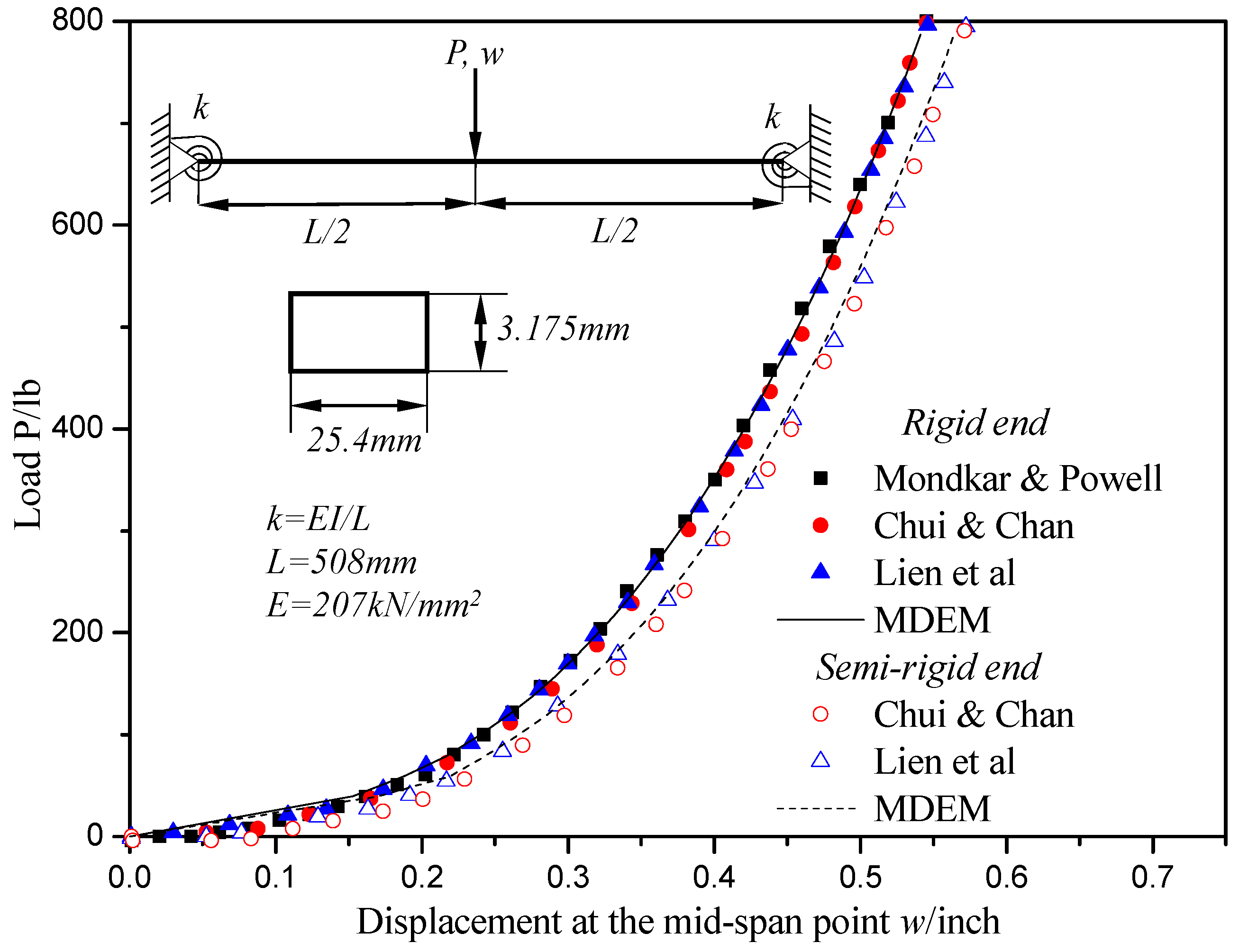
The schematic configuration of a beam with elastic ends is displayed in Figure 7. The properties of the beam are listed as follow: cross section A = 25.4 mm × 3.175 mm, length L = 508 mm, and elastic modulus E = 207 GPa. A gradually increasing concentrated load P is applied at the mid-span point. Mondkar and Powell [31] as well as Yang and Saigal [32] analyzed the static and dynamic response of the beam with fixed ends. The static and dynamic response of the beam with semi-rigid ends was investigated by Chui and Chan [13] and Lien et al. [20] using the conventional FEM and the VFIFE, respectively. The rotation-resistant stiffness k of the semi-rigid ends is EI/L.
In this study, the beam was represented by 51 particles (i.e., 50 contact elements). The ends were modeled as rigid and semi-rigid in the rotational direction, respectively. The semi-rigid behavior was simulated by the contact elements at the ends with the stiffness in the rotational direction of 49EI/L which was obtained according to Table 1. Figure 7 shows that the load-displacement curves of the modified MDEM are consistent with the published results (Mondkar and Powell [29]; Chui and Chan [13]; Lien et al. [21]); the stiffness of the ends has a significant effect on structural stiffness, and the stiffness of the beam with semi-rigid ends is obviously reduced. In addition, the stiffness of the beam increases with an increase of the load, the reason is that the tensile reaction at the supports induces the axial tension arising in the beam.
The dynamic response analysis of the same beam was further performed. A sudden load was applied at the mid-span point, that is, the load p was linearly increased to pmax (640 lb) within a very short time (10 μs), and then the pmax is maintained until the calculation ended (), as shown in Figure 8. During the analysis, the material was assumed to be perfectly elastic, and the viscous damping was ignored. It can be found from Figure 8 that the analysis results of the modified MDEM is identical with published results, and the minor error is due to the inevitable numerical method itself. Moreover, the stiffness of the ends affects significantly on the period and amplitude of displacement time history curves. The structural stiffness decreases with semi-rigid supports, whereas both the period and amplitude increase accordingly.
4.3. Static and Dynamic Response Analysis of Steel Frames with Linear Semi-Rigid Connections
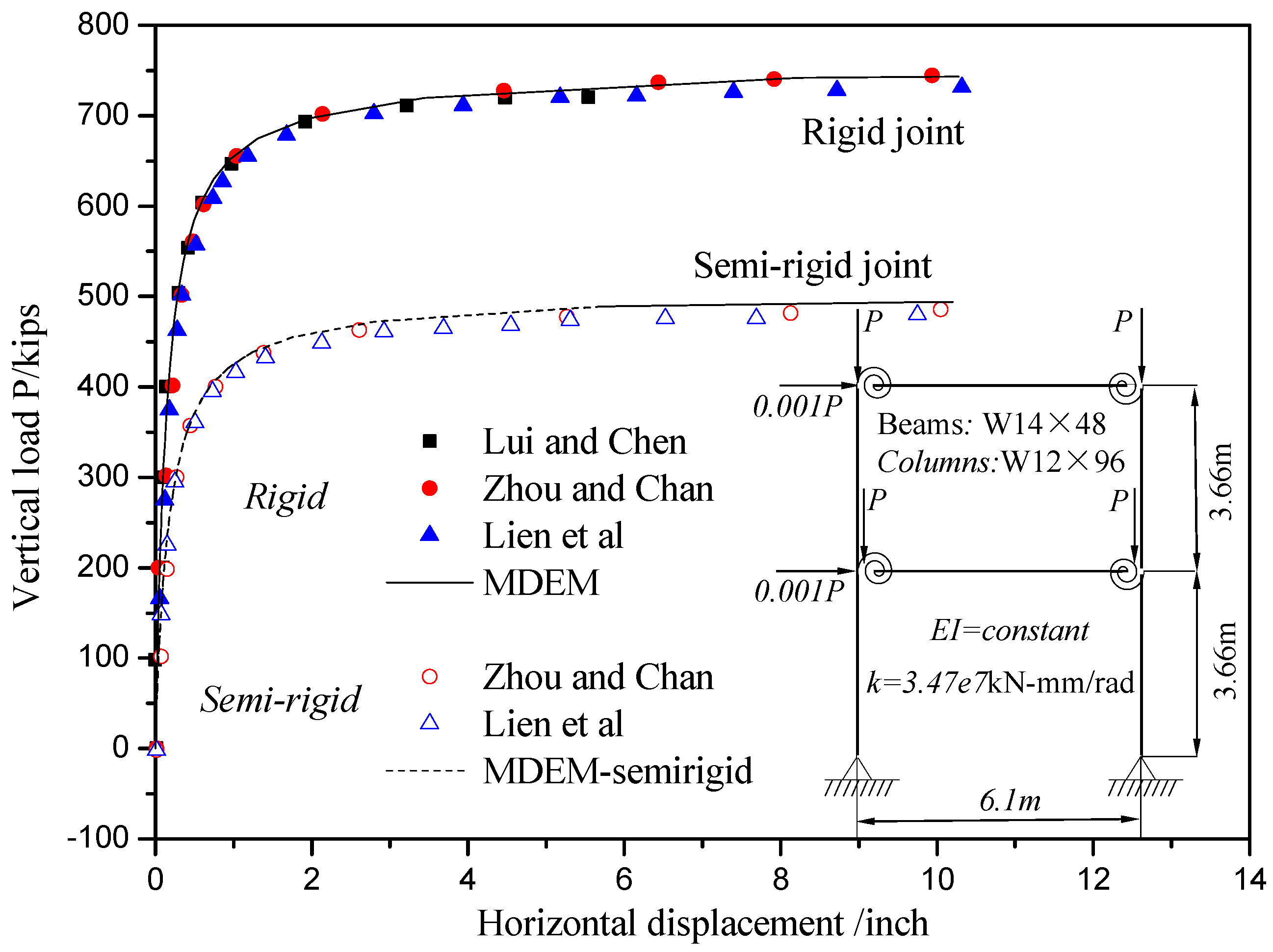
Figure 9 displays the configuration and loading of a single-bay two-story steel frame with W14 × 48 steel beams and W12 × 96 steel columns. The elastic modulus is 200 GPa. A vertical concentrated load P was applied to four joints, meanwhile a horizontal load 0.01p was added to consider the geometric imperfection or wind load. Several studies (Lui and Chen [9], Zhou and Chan [12]; Lien et al. [20]) carried out stability analysis of the structure in the two cases of rigid and semi-rigid connections using different simulation methods. In the above analysis, the bending-resistant stiffness of semi-rigid beam-column joints was taken to be 3.48 × 10⁷ kN-m/rad.
The MDEM discretized the single-bay two-story steel frame into 28 particles (i.e., 28 contact elements). Of these, each column was represented by 4 contact elements while every beam by 6 contact elements. The bending-resistant stiffness of the contact elements at the beam ends was modified to be 3.48 × 10⁷ kN-m/rad according to Table 1. The horizontal displacement of steel frames with linear semi-rigid joints is shown in Figure 9. The figure shows that the load-displacement relationship of the modified MDEM is in a good agree with the published results. Additionally, the effect of semi-rigid connections on the structural behavior is great, and structural loading capacity may be overestimated if semi-rigid connections are ignored.
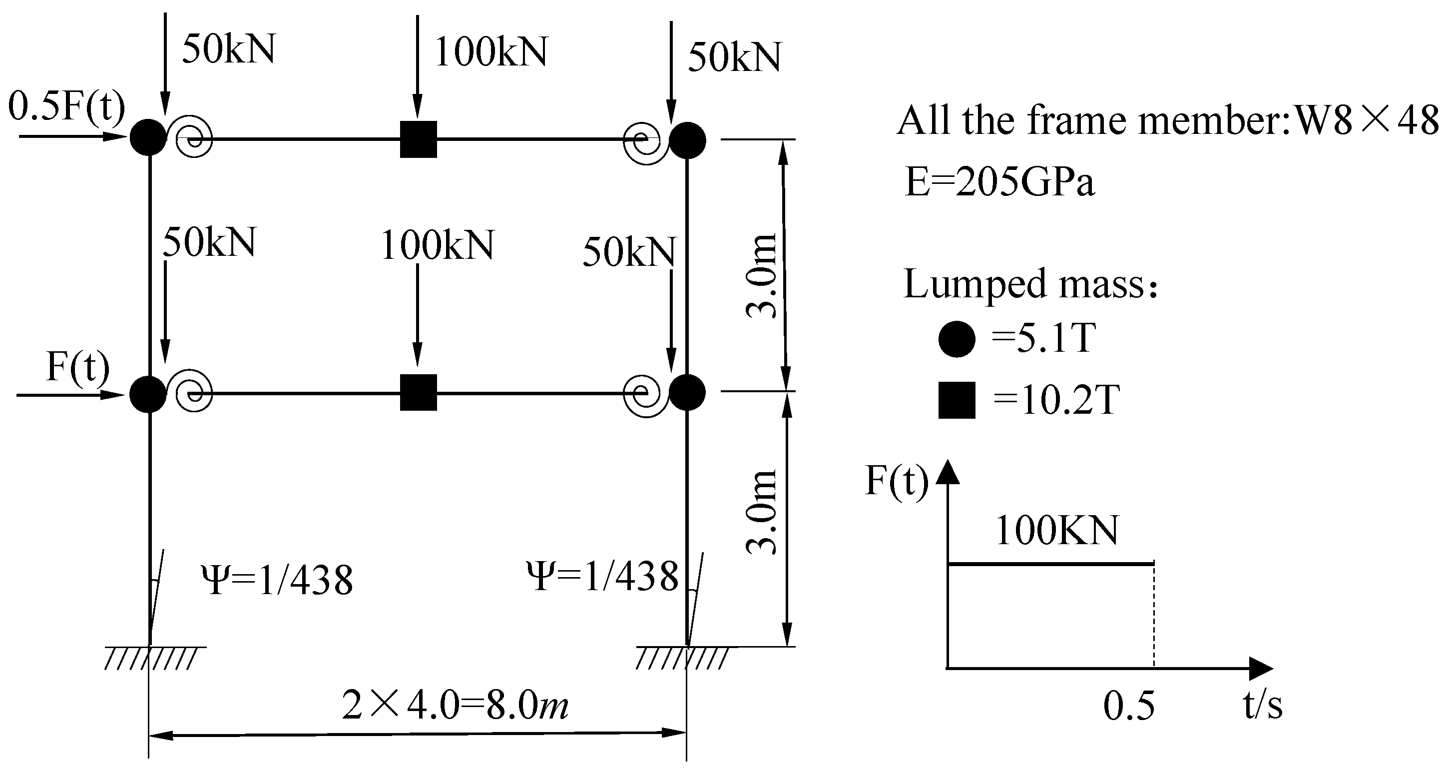
Another single-bay two-story steel frame with linear semi-rigid joints was adopted to analyze the dynamic response. The configuration and loading of this structure are shown in Figure 10. All the beams and columns are W8 × 48 and the Young’s modulus is 205 GPa. The material of all the frame members was assumed to be perfectly elastic and the viscous damping was ignored. The initial geometric imperfection ψ was taken to be 1/438 rad. The lumped masses of 5.1 T and 10.2 T were set at the top of the columns and in the middle of the beams, respectively. The stiffness of semi-rigid connections was 23,000 kN-m/rad. In this study, each beam was simulated by 9 particles (i.e., 8 contact elements), while every column was discretized into 4 particles (3 contact elements). As the stiffness of each frame member is same, the bending-resistant stiffness of the contact elements at the semi-rigid joints can be determined to be 11,500 kN-m/rad by Equation (13) not Table 1. The vertical static loads of 50 KN and 100 KN were first applied on the beam-column joints and in the middle of beams to consider the second-order effects, and then the horizontal forces were added suddenly at each floor during 0.5 s until the calculation ended. The horizontal displacement on the top is shown in Figure 11. The comparison indicates the displacement responses of the MDEM and existing results (Chan and Chui [13], Nguyen and Kim [18]) are consistent, and the influence of semi-rigid connections on the periods and the amplitudes of displacement responses of steel frames is more significant as well as the amplitude increase is up to 60%.
4.4. Snap-Through Buckling Analysis of the Williams Toggle Frame with Linear Semi-Rigid Connections and Supports
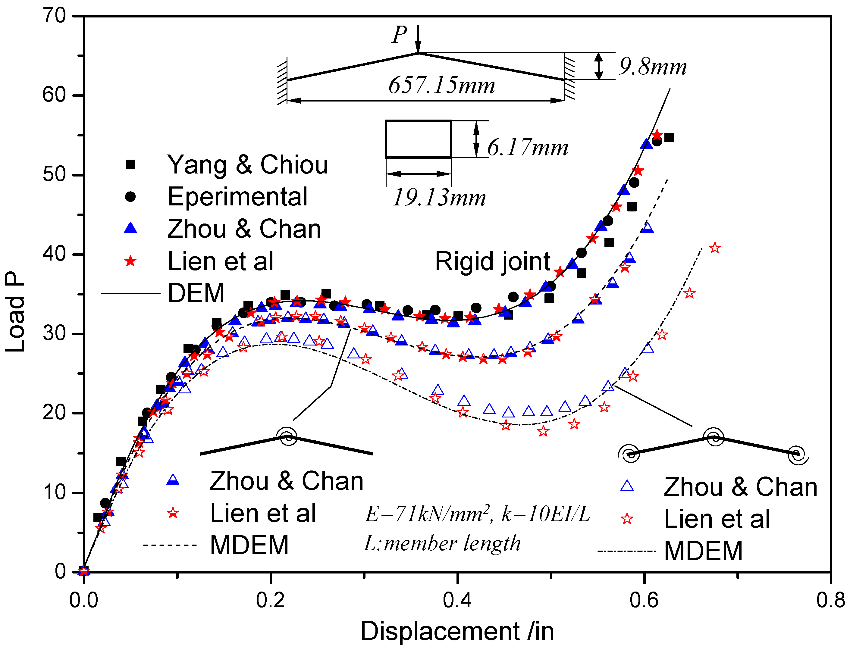
The Williams Toggle frame is frequently taken as a typical example for snap-through buckling analysis. The structure has the obviously nonlinear bifurcation instability, that is, each bifurcation point may have one or more equilibrium paths and each path represents the extreme point instability or snap instability [12,33]. Many researchers (Zhou and Chan [12], Lien et al. [20]) performed static stability analysis of the steel frame with linear semi-rigid connections and supports, and the bending-resistant stiffness of each semi-rigid connection or support k is 10EI/L. The properties of the Williams Toggle frame is as follow: cross section A = 19.13 mm × 6.17 mm; the Young’s modulus E = 71 GPa.
Negative or zero structural stiffness may occur at the instant of buckling, resulting that special treatments for conventional FEM is necessary to investigate snap-through buckling behavior. In the FEM, the most commonly used approach is the arc-length method [26]. However, in the MDEM, no negative or zero stiffness issues occur because of no assembly of stiffness matrix, and only displacement control method need be applied to trace the complete equilibrium path. In this study, each member was discretized into 13 particles (i.e., 12 contact elements), and the applied displacement increment was . The bending-resistant stiffness of the contact elements at the semi-rigid joints was determined to be 7EI/L by Table 1. Snap-through buckling analyses of the MDEM and the existing results (Yang and Chiou [31]; Experimental result [34]; Zhou and Chan [12]; Lien et al. [20]) are displayed in Figure 12. The comparison shows that the modified MDEM can accurately carried out the snap-through buckling analysis of the Williams Toggle frame with semi-rigid connections and supports. Furthermore, semi-rigid connections and support have a significant effect on the critical load and post-buckling behavior.
4.5. Static Analysis of a Steel Portal Frame with Bilinear Semi-Rigid Connections
The bilinear semi-rigid connection model presented by Keulen et al. [8] is adopted to simulate the nonlinear behavior of semi-rigid connections. Figure 13 shows the detail configuration of a steel portal frame. The beam-column joints are bolted by flush endplates, which are obviously nonlinear semi-rigid connections. Keulen et al. [8] carried out the second-order elastic-plastic analysis using the ANSYS software (ANSYS, Inc., Pittsburgh, PA, USA). Del Savio et al. [35] and Lien et al. [20] were further performed static analysis using different numerical methods.
The steel portal frame was made of S335 steel, IPE360 and HEA260 sections [8]. The span and height were 7.2 m and 3.6 m, respectively. A concentrated load F was applied at the joints and in the beam, as shown in Figure 13. The horizontal loads was set to be to consider the initial geometrical imperfection and wind load, where was taken to be 0.1, 0.15, 0.2, 0.3 and 0.5 successively. The semi-rigid supports was assumed to be perfectly elastic-plastic, its initial stiffness is 23,000 kN-m/rad, and the moment capacity was 200 kN-m. The moment-rotation relation of beam-column joints, proposed by Keulen et al. [8], is shown in Figure 14. The joints were simulated using the full characteristic nonlinear model and a bilinear model. The connection model applied in this study is the bilinear model in Figure 14.
In this study, there were 36 particles and 36 contact elements for this structure, and the radius of each particle was 0.2 m. The bending-resistant stiffness of the contact elements at the semi-rigid joints was obtained by Equation (13), while that of the contact elements at the supports could be determined according to Table 1. The comparison given in Figure 15 shows that the modified MDEM can accurately simulate the nonlinear behavior of semi-rigid connections and supports of a single-story steel portal frame. Moreover, the connection behavior obtained using simplified half initial secant stiffness approach has a good agreement with the full characteristic analysis. Taking = 0.2 as an example, the load-moment curves of joints and supports are shown in Figure 16. It can be found from the figure that the semi-rigid beam-column joint on the right top first reached the plastic state, and a plastic hinge formed.
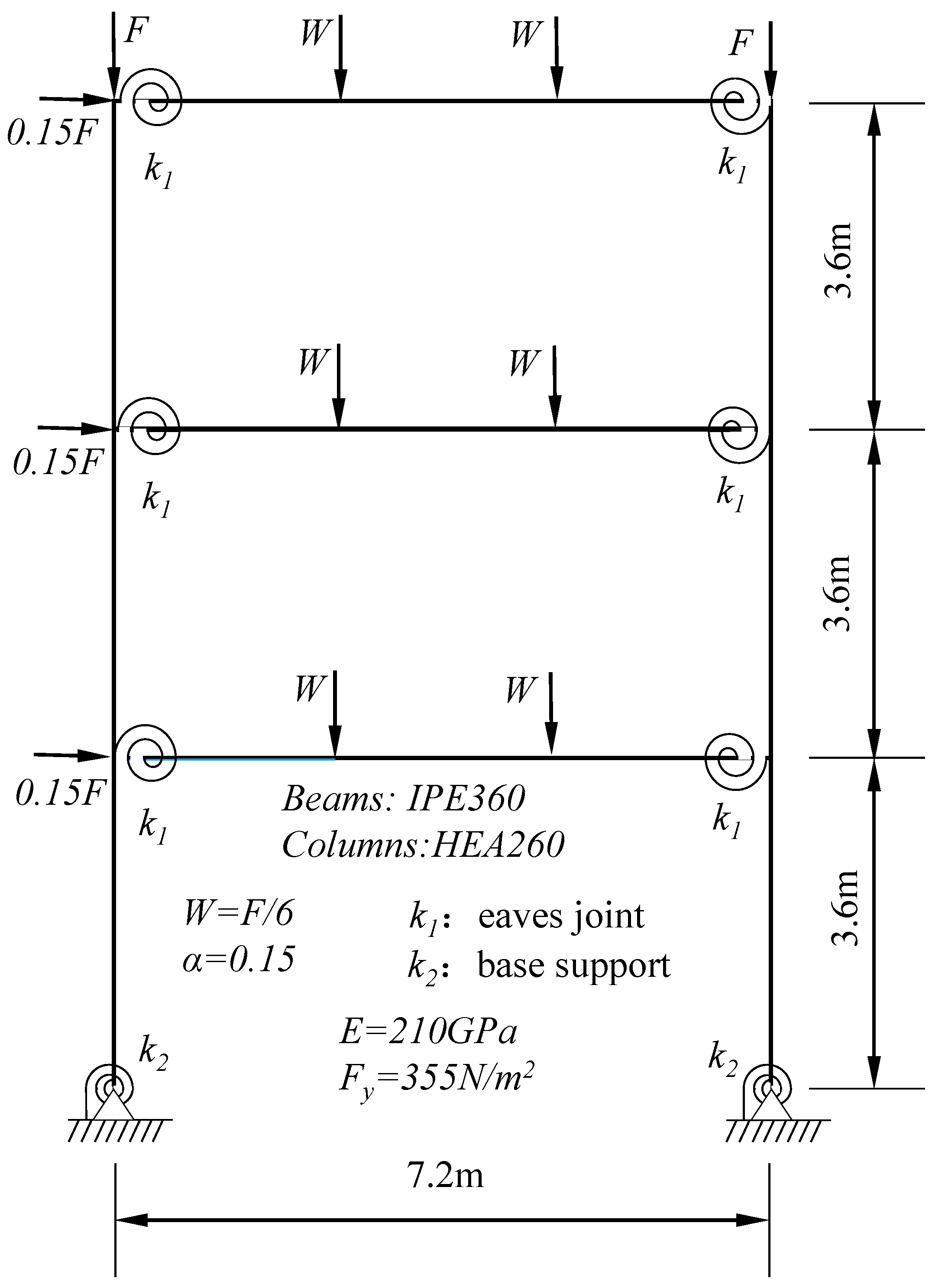
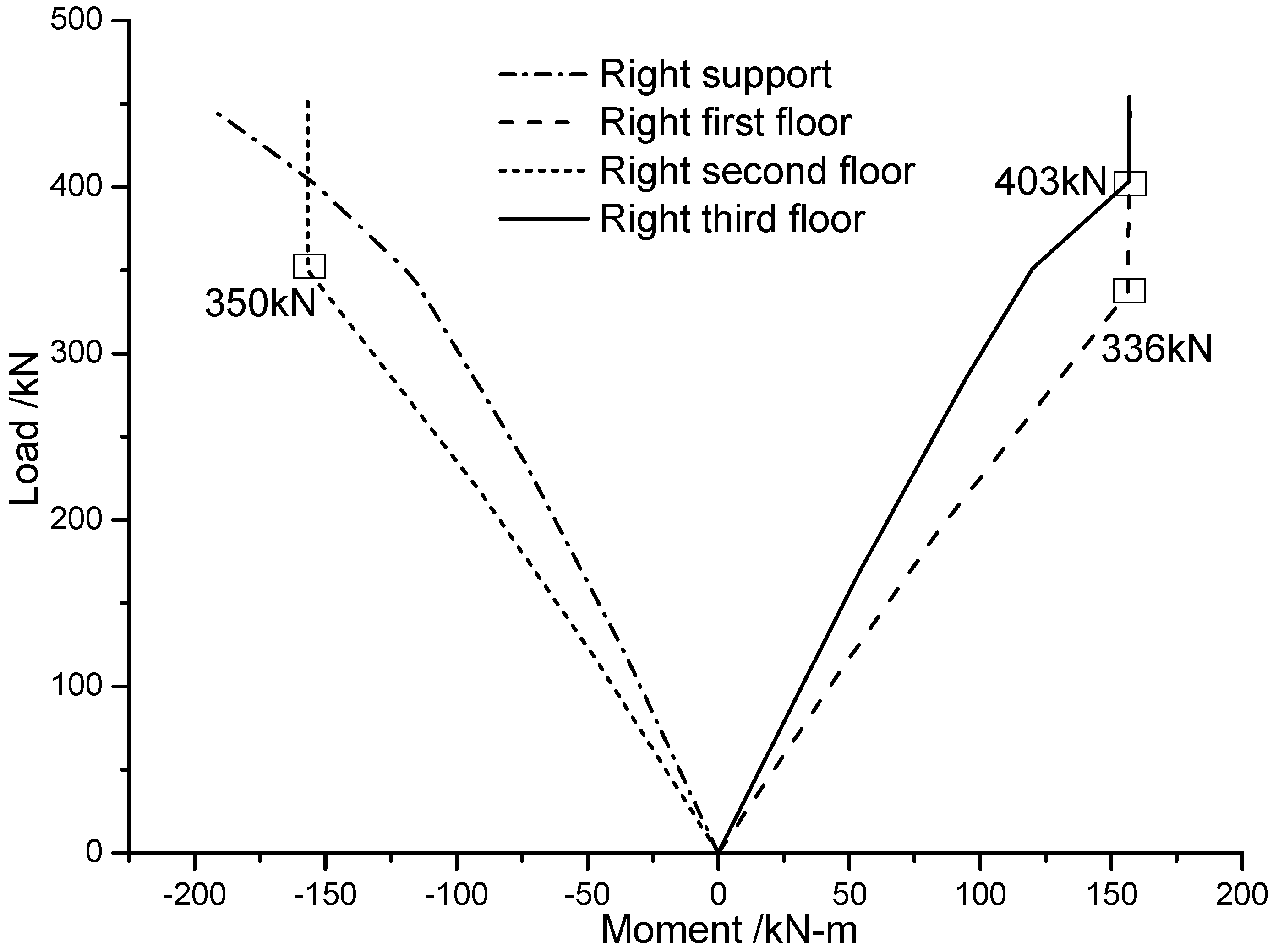
The static analysis of a three-story steel portal frame was further performed, as shown in Figure 17. The nonlinear behavior of the beam-column joint was simulated using the bilinear model simplified by the half initial secant stiffness approach. The procedure of determining the bending-resistant stiffness of contact elements at the semi-rigid connection was the same as the single-story frame. The horizontal load was set to . Figure 18 shows the moment-rotation relation of the beam-column joint. The analysis result of the MDEM and the published results (Keulen et al. [8] and Del Savio et al. [33]) are displayed in Figure 19. The figure indicates that the modified MDEM possesses considerable accuracy for the nonlinear behavior simulation of the semi-rigid connection of multi-story steel portal frames. Additionally, from the load-moment curves on the right joints and supports (Figure 20), it is found that for three-story steel portal frame with semi-rigid joints and supports, the beam-column joint on the right side of first floor reached the plastic state and a plastic hinge formed. When the load continues to increase to 336 kN and 403 kN accordingly, the plastic hinge in turn occurred at the beam-column joints on the right side of second floor and third floor.
4.6. Dynamic Analysis of the Two-Span, Six-Story Vogel Steel Frame with Nonlinear Semi-Rigid Connections
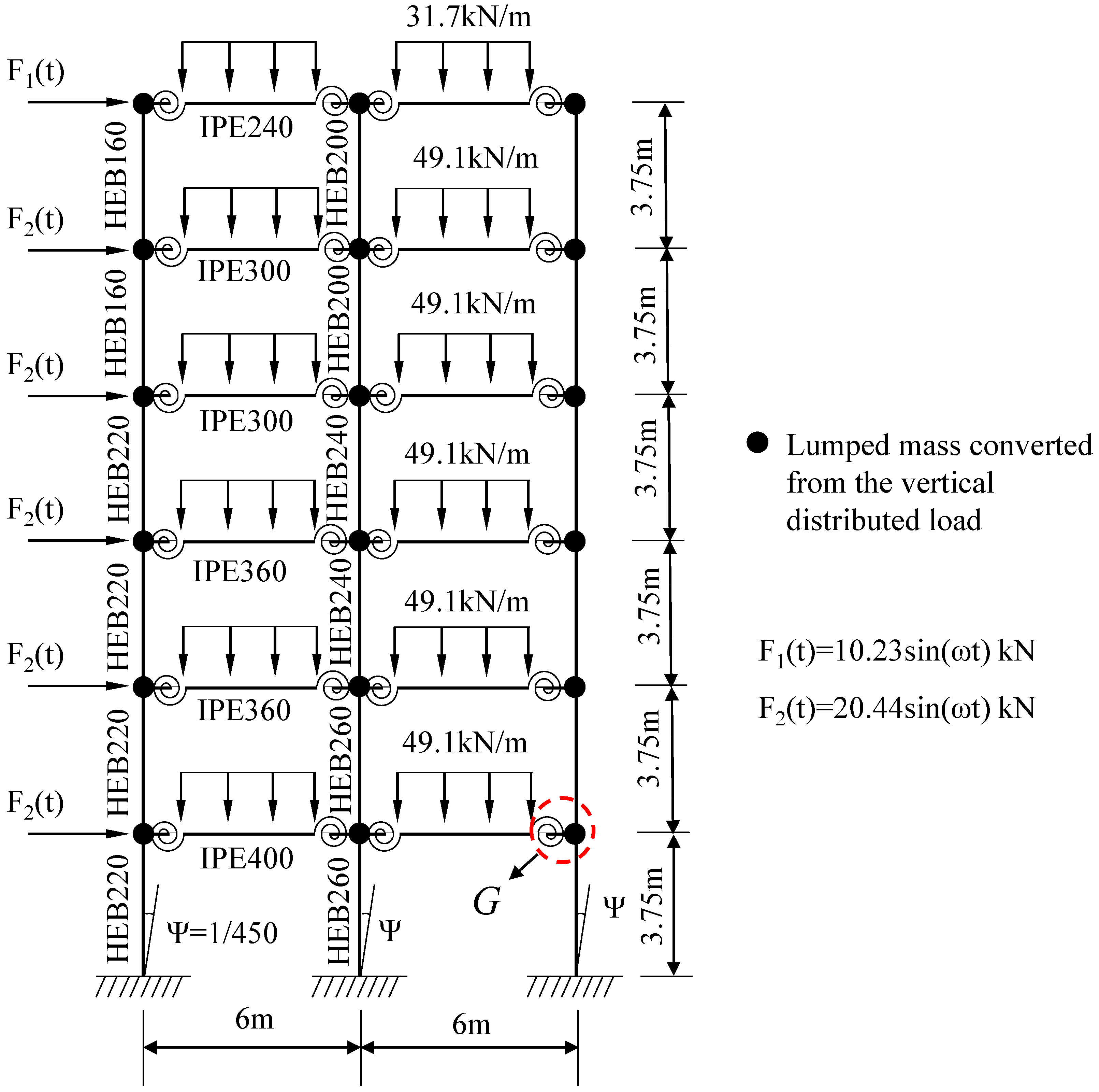
Figure 21 shows the configuration and loading of the two-span, six-story Vogel steel frame. Each span and each floor height were 6 m and 3.75 m, respectively. The section types of beams were IPE240, IPE300, IPE360 and IPE400, while the section types of columns were HEB160, HEB200, HEB220, HEB240 and HEB260. An initial geometric imperfection of 1/450 was taken into account. The distributed loads of 31.7 kN/m and 49.1 kN/m applied on the beams were converted into lumped masses at the joints. The elastic modulus and the Poisson ratio were 205 GPa and 0.3. In order to more intuitively study the energy consumption of semi-rigid connections, the material of all the frame members was assumed to be perfectly elastic, and the viscous damping was ignored.
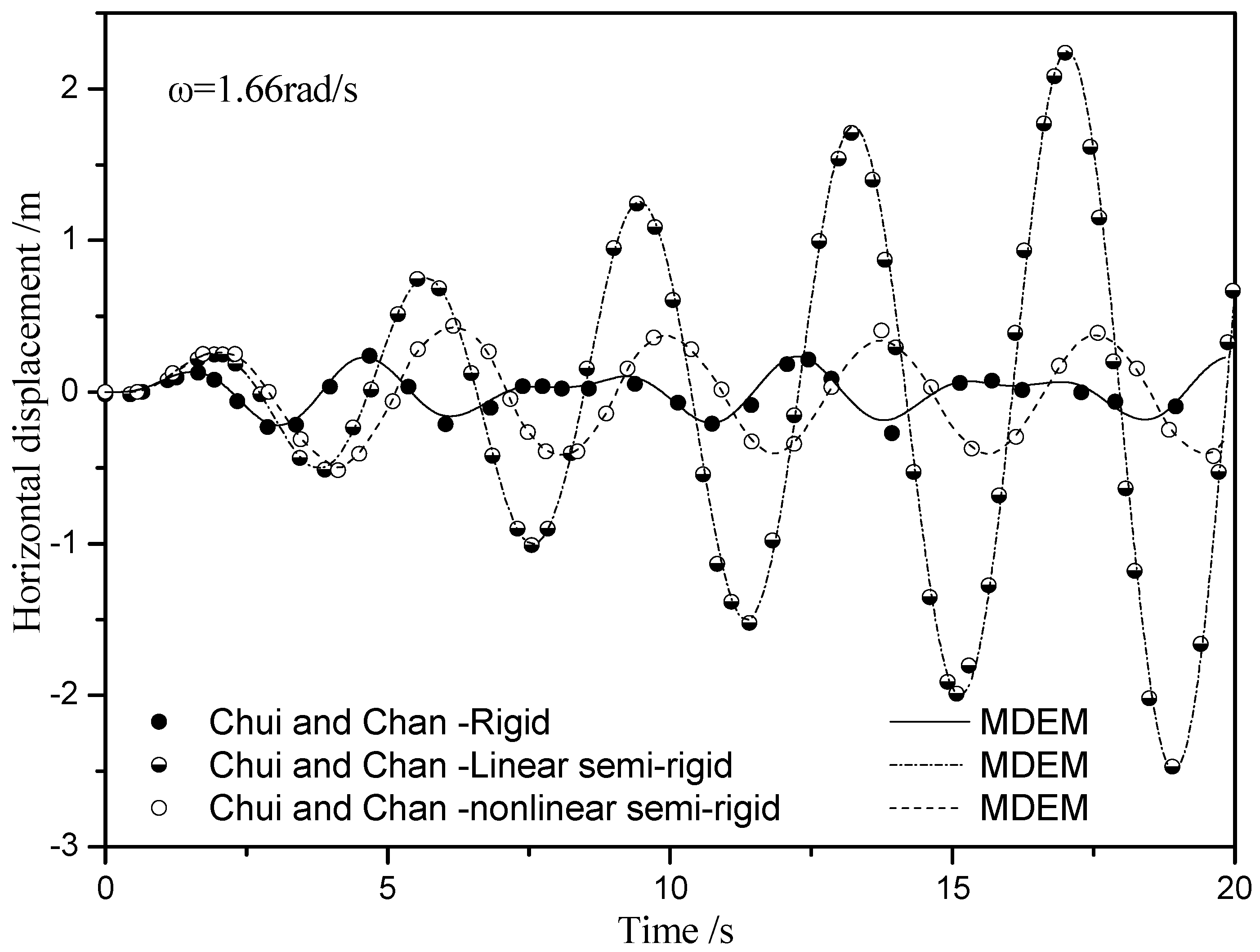
In this study, there were 10 contact elements for each column while 16 contact elements for every beam. The nonlinear behavior of the semi-rigid connection was simulated by the Richard-Abbott model. The parameters of the model were as follow: = 12336.86; = ; = ; . The instantaneous stiffness of the contact elements at semi-rigid connections was determined by Equations (13) and (15). The frequency of the dynamic force is , which was close to the fundamental natural frequency of this structure. The dynamic response analysis of the frame was performed at three cases of rigid connection, linear semi-rigid connection and nonlinear semi-rigid connection, as shown in Figure 22. The comparison of the numerical results obtained using the modified MDEM and those presented by Chui and Chan [13] illustrates that the two match well, and the modified MDEM can accurately capture the nonlinear behavior of the semi-rigid connection. In addition, it is observed that resonance occurs in the frames with rigid or linear semi-rigid connections, but not in the frame with nonlinear semi-rigid connections, the reason is that the hysteresis damping of the nonlinear connection causes energy dissipation (Figure 23).
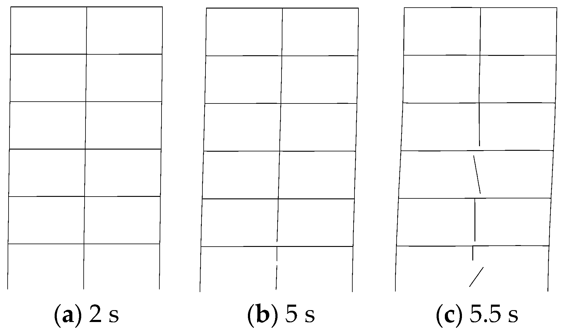
In order to simulate the collapse behavior of this structure, the ultimate strain was taken as the fracture criterion. The material was elastic during the calculation, and the beam-column joints were assumed to be linear semi-rigid connections. The sine wave with the frequency of 1.66 rad/s was applied. The failure processes of steel frames with different connections are shown in Figure 24 and Figure 25. It can be seen from the figures that the displacement at the top of the frame with semi-rigid connection is obviously larger than that of the frame with rigid connection, and the fracture time of the frame with rigid connection is earlier. It also indicates that the ductility of the semi-rigid connection is better than that of rigid connection. Steel frames with semi-rigid connections have more anti-collapse ability than those with rigid connection.
5. Conclusions
- (1)
- This paper presented an effective numerical approach for static and dynamic behavior simulation of steel frames with semi-rigid joints based on the Member Discrete Element Method (MDEM). In the MDEM, a structure is discretized into a set of finite rigid particles, as well as geometric nonlinearity and fracture behaviors can be naturally captured. A virtual spring element without actual length is applied to simulate the semi-rigid connection. On this basis, the modified formula of the contact element stiffness at the semi-rigid connection is derived. Finally, the numerical approach proposed is verified by complex behaviors of steel frames with semi-rigid connections such as geometric nonlinearity, snap-through buckling, dynamic responses and fracture. In addition, compared with other numerical approaches taking the FEM as a representation, the approach proposed is simple and feasible for simulating the semi-rigid connections because the zero-length spring element is not directly involved in the calculation.
- (2)
- The comparison of the analysis results of the proposed approach and the existing researches shows that the modified MDEM can accurately capture linear and nonlinear behaviors of semi-rigid connections. Some common conclusions can be drown as follow: the semi-rigid connections may significantly reduce structural stiffness, and structural bearing capacity under static loading will be overestimated if the semi-rigid connections are ignored; When the frequency of dynamic load applied is close to structural fundamental frequency, resonance occurs in the frames with rigid or linear semi-rigid connections, but not in the frame with nonlinear semi-rigid connections, the reason is that the hysteresis damping of the nonlinear connection causes energy dissipation. Fracture behavior analysis also indicates that frames with semi-rigid connection possess more anti-collapse capacity.
- (3)
- The MDEM can avoid the difficulties of finite element method (FEM) in dealing with strong nonlinearity and discontinuity. A unified computational framework is applied for static and dynamic analyses. The method is simple and generally good, which is an effective tool to investigate complex behaviors of steel frames with semi-rigid connections. In the follow-up study, material nonlinearity will be taken into account to simulate the collapse process of steel frames with semi-rigid connections under strong earthquake or impact loading action.
Acknowledgments
This work is supported by the National Science Found for Distinguished Young Scholars of China (Grant No. 51125031) and A Project Funded by the Priority Academic Program Development of Jiangsu Higher Education Institutions (CE02-1-31).
Author Contributions
Jihong Ye and Lingling Xu modified the Member Discrete Element Method, analyzed the numerical results, and wrote the paper.
Conflicts of Interest
The authors declare no conflict of interest.
References
- Nguyen, P.-C.; Kim, S.-E. Second-order spread-of-plasticity approach for nonlinear time-history of space semi-rigid steel frames. Finite Elem. Anal. Des. 2015, 105, 1–15. [Google Scholar] [CrossRef]
- Abdalla, K.M.; Chen, W.F. Expanded database of semirigid steel connections. Comput. Struct. 1995, 56, 553–564. [Google Scholar] [CrossRef]
- Brown, N.D.; Anderson, D. Structural properties of composite major axis end plate connections. J. Constr. Steel Res. 2001, 57, 327–349. [Google Scholar] [CrossRef]
- Chen, W.F.; Kishi, N. Semirigid steel beam-to-column connections- data-base and modeling. J. Struct. Eng. ASCE 1989, 115, 105–119. [Google Scholar] [CrossRef]
- Richard, R.M.; Abbott, B.J. Versatile elastic-plastic stress–strain formula. J. Eng. Mech. Div. ASCE 1975, 101, 511–515. [Google Scholar]
- Wang, X.; Ye, J.; Yu, Q. Improved equivalent bracing model for seismic analysis of mid-rise CFS structures. J. Constr. Steel Res. 2017, 136, 256–264. [Google Scholar] [CrossRef]
- Eurocode 3. Design of Steel Structures-Joints Inbuilding Frames; ENV-1993-1-1:1992/A2; Annex, J., Ed.; European Committee for Standardization (CEN): Brussels, Belgium, 1998. [Google Scholar]
- Keulen, D.C.; Nethercot, D.A.; Snijder, H.H.; Bakker, M.C.M. Frame analysis incorporating semirigid joint action: Applicability of the half initial secant stiffnes approach. J. Constr. Steel Res. 2003, 59, 1083–1100. [Google Scholar] [CrossRef]
- Lui, E.M.; Chen, W.F. Analysis and behavior of flexibly-jointed frames. Eng. Struct. 1986, 8, 107–118. [Google Scholar] [CrossRef]
- Ho, W.M.G.; Chan, S.L. Semibifurcation and bifurcation analysis of flexibly connected steel frames. J. Struct. Eng. ASCE 1991, 117, 2298–2318. [Google Scholar] [CrossRef]
- Yau, C.Y.; Chan, S.L. Inelastic and stability analysis of flexibly connected steel frames by springs-in-series model. J. Struct. Eng. 1994, 120, 2803–2819. [Google Scholar] [CrossRef]
- Zhou, Z.H.; Chan, S.L. Self-equilibrating element for second-order analysis of semirigid jointed frames. J. Eng. Mech. 1995, 121, 896–902. [Google Scholar] [CrossRef]
- Chui, P.P.T.; Chan, S.L. Transient response of moment-resistant steel frames with flexible and hysteretic joints. J. Constr. Steel Res. 1996, 39, 221–243. [Google Scholar] [CrossRef]
- Chan, S.L.; Chui, P.T. Non-Linear Static and Cyclic Analysis of Steel Frames with Semi-Rigid Connections; Elsevier: Amsterdam, The Netherlands, 2002. [Google Scholar]
- Sophianopoulos, D.S. The effect of joint flexibility on the free elastic vibration characteristics of steel plane frames. J. Constr. Steel Res. 2003, 59, 995–1008. [Google Scholar] [CrossRef]
- Li, T.Q.; Choo, B.S.; Nethercot, D.A. Connection element method for the analysis of semirigid frames. J. Constr. Steel Res. 1995, 32, 143–171. [Google Scholar] [CrossRef]
- Raftoyiannis, I.G. The effect of semi-rigid joints and an elastic bracing system on the buckling load of simple rectangular steel frames. J. Constr. Steel Res. 2005, 61, 1205–1225. [Google Scholar] [CrossRef]
- Nguyen, P.-C.; Kim, S.-E. Nonlinear elastic dynamic analysis of space steel frames with semi-rigid connections. J. Constr. Steel Res. 2013, 84, 72–81. [Google Scholar] [CrossRef]
- Nguyen, P.-C.; Kim, S.-E. Nonlinear inelastic time-history analysis of three-dimensional semi-rigid steel frames. J. Constr. Steel Res. 2014, 101, 192–206. [Google Scholar] [CrossRef]
- Lien, K.H.; Chiou, Y.J.; Hsiao, P.A. Vector form intrinsic finite-element analysis of steel frames with semi-rigid joints. J. Struct. Eng. 2012, 138, 327–336. [Google Scholar] [CrossRef]
- Ying, Y.; Xing, Y.Z. Nonlinear dynamic collapse analysis of semi-rigid steel frames based on the finite particle method. Eng. Struct. 2016, 118, 383–393. [Google Scholar]
- Ye, J.; Qi, N. Progressive collapse simulation based on DEM for single-layer reticulated domes. J. Constr. Steel Res. 2017, 128, 721–731. [Google Scholar]
- Cundall, P.A.; Strack, O.D.L. A discrete element model for granular assemblies. Geotechnique 1979, 29, 47–65. [Google Scholar] [CrossRef]
- Ye, J.; Qi, N. Collapse process simulation of reticulated shells based on coupled DEM/FEM model. J. Build. Struct. 2017, 38, 52–61. (In Chinese) [Google Scholar]
- Qi, N.; Ye, J. Nonlinear dynamic analysis of space frame structures by discrete element method. Appl. Mech. Mater. 2014, 638–640, 1716–1719. [Google Scholar] [CrossRef]
- Xu, L.; Ye, J. DEM algorithm for progressive collapse simulation of single-layer reticulated domes under multi-support excitation. J. Earthq. Eng. 2017. [Google Scholar] [CrossRef]
- Wang, X.C. Finite Element Method; Tsinghua University Press: Beijing, China, 2003. [Google Scholar]
- Qi, N.; Ye, J.H. Geometric nonlinear analysis with large deformation of member structures by discrete element method. J. Southeast Univ. (Nat. Sci. Ed.) 2013, 43, 917–922. (In Chinese) [Google Scholar]
- Lynn, K.M.; Isobe, D. Finite element code for impact collapse problem. Int. J. Numer. Method. Eng. 2007, 69, 2538–2563. [Google Scholar] [CrossRef]
- Ramberg, W.; Osgood, W.R. Description of Stress-Strain Curves by Three Parameters; National Advisory Committee for Aeronautics: Washington, DC, USA, 1943. [Google Scholar]
- Mondkar, D.P.; Powell, G.H. Finite element analysis of nonlinear static and dynamic response. Int. J. Numer. Method. Eng. 1977, 11, 499–520. [Google Scholar] [CrossRef]
- Yang, T.Y.; Saigal, S. A simple element for static and dynamic response of beams with material and geometric nonlinearities. Int. J. Numer. Method. Eng. 1984, 20, 851–867. [Google Scholar] [CrossRef]
- Yang, Y.B.; Chiou, H.T. Analysis with beam elements. J. Eng. Mech. 1987, 113, 1404–1419. [Google Scholar] [CrossRef]
- Williams, F.W. An approach to the nonlinear behaviour of the members of a rigid jointed plane framework with finite deflection. Q. J. Mech. Appl. Maths 1964, 17, 451–469. [Google Scholar] [CrossRef]
- Del Savio, A.A.; Andrade, S.A.L.; Vellasco, P.C.G.S.; Martha, L.F. A nonlinear system for semirigid steel portal frame analysis. In Proceedings of the 7th International Conference on Computational Structures Technology, Tecnologiaem Computação Gráfica, Rio de Janeiro, Brazil, 10–11 January 2004; Volume 1, pp. 1–12. [Google Scholar]
Figure 1.
Discretization procedure of a plane steel frame.

Figure 2.
MDEM (Member Discrete Element Method) model of a simple steel frame.

Figure 3.
Zero-length spring element at a semi-rigid connection.

Figure 4.
Independent hardening model.

Figure 5.
MDEM flowchart for static and dynamic analysis of steel frames with semi-rigid connections.
Figure 5.
MDEM flowchart for static and dynamic analysis of steel frames with semi-rigid connections.
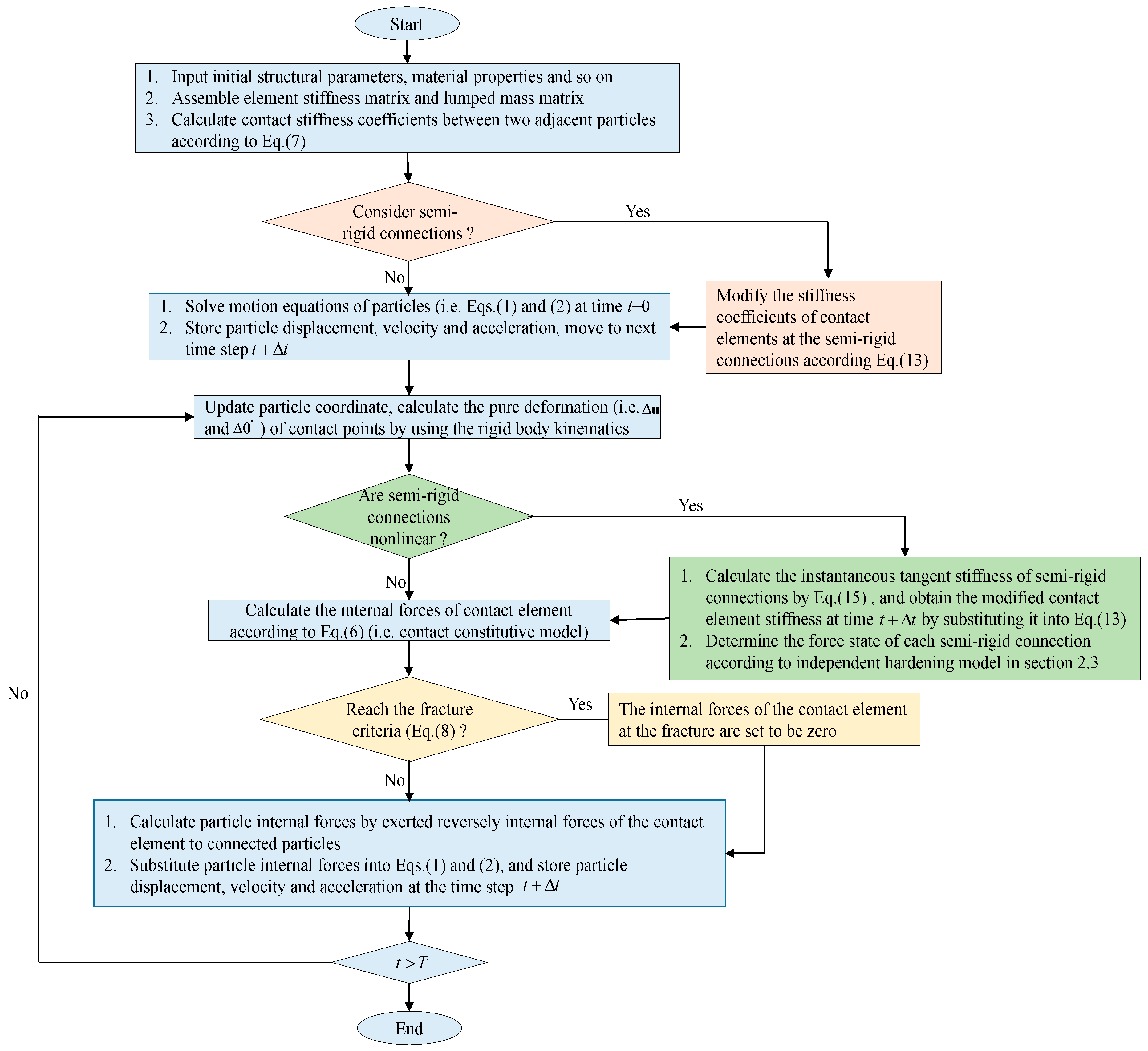
Figure 6.
Load-displacement curves at the free end of the column.

Figure 7.
Displacement at the mid-span point of the beam under static loading.

Figure 8.
Displacement time history curves at the mid-span point of the beam under sudden loading.
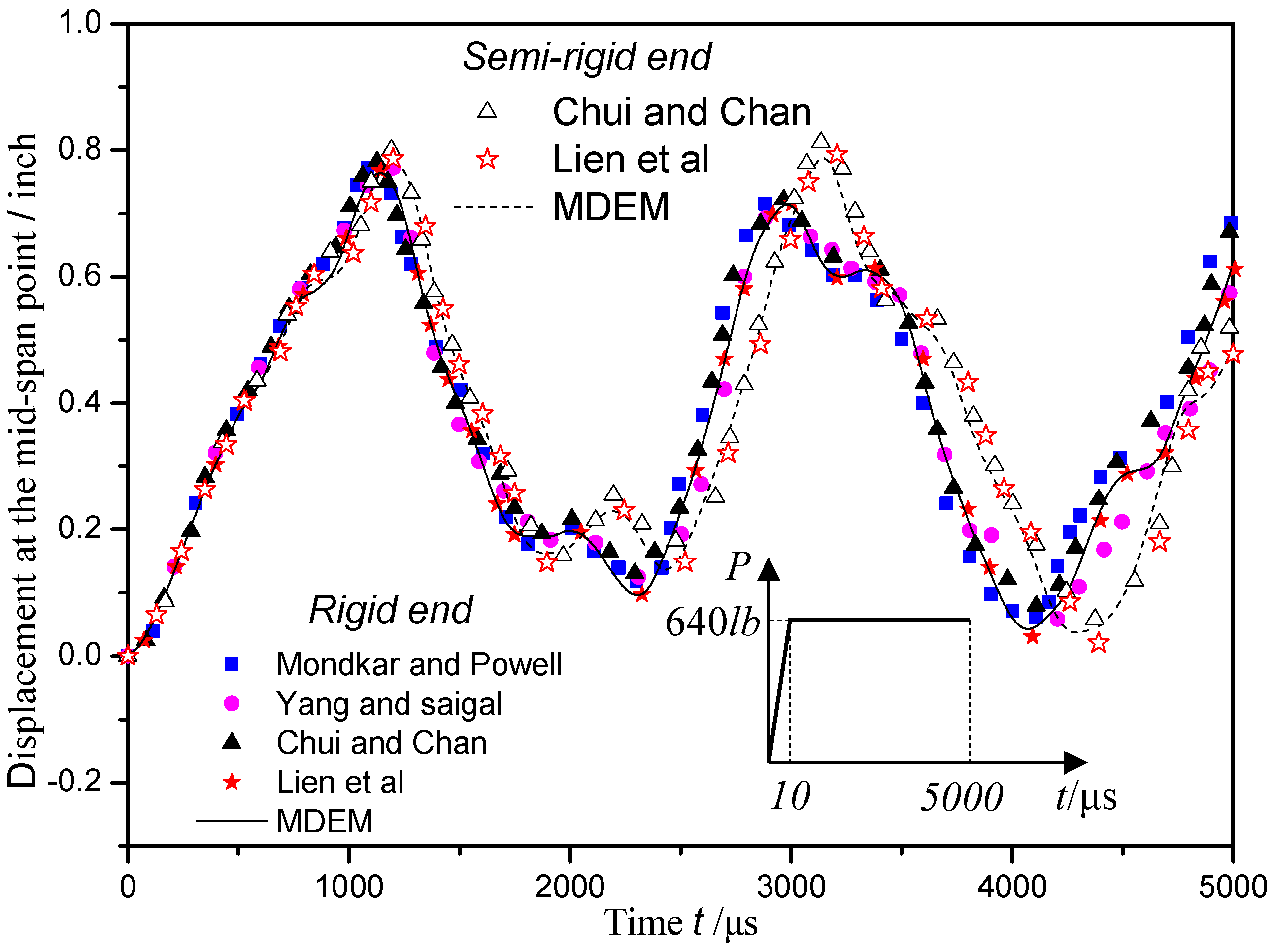
Figure 9.
Horizontal displacement of steel frames with linear semi-rigid joints.

Figure 10.
The configuration and loading of the structure adopted in dynamic analysis.

Figure 11.
Displacement time history curves of a steel frame with linear semi-rigid connections.
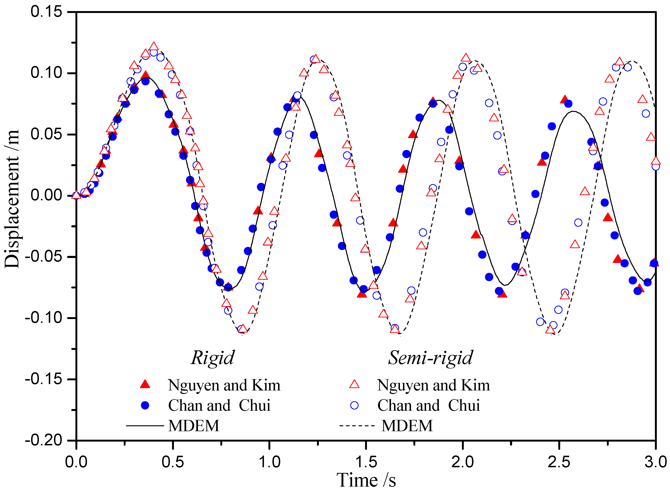
Figure 12.
Displacement response of the Williams Toggle frame with linear semi-rigid connections and supports.
Figure 12.
Displacement response of the Williams Toggle frame with linear semi-rigid connections and supports.

Figure 13.
A steel portal frame with semi-rigid connections and supports.
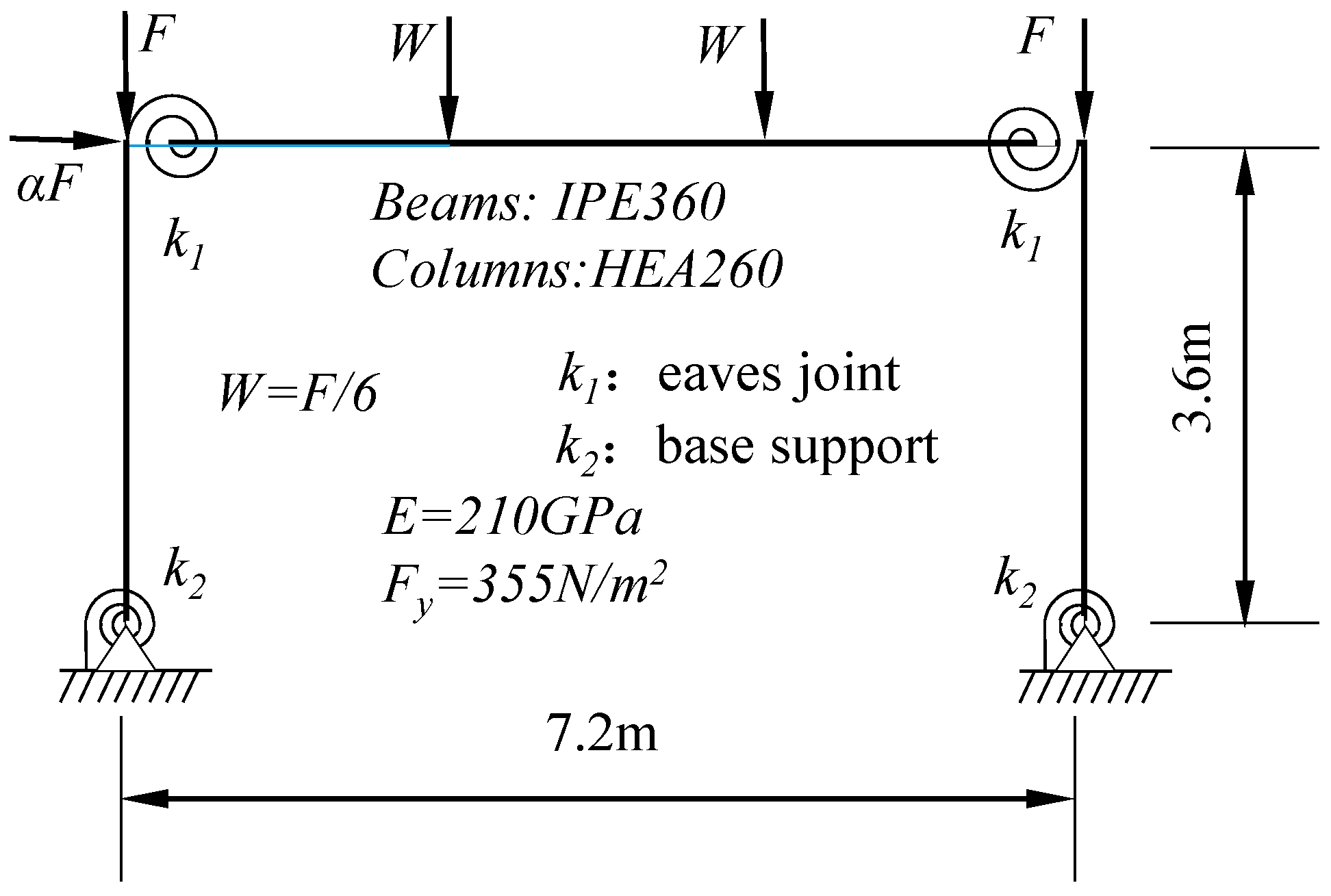
Figure 14.
Load-moment curves.
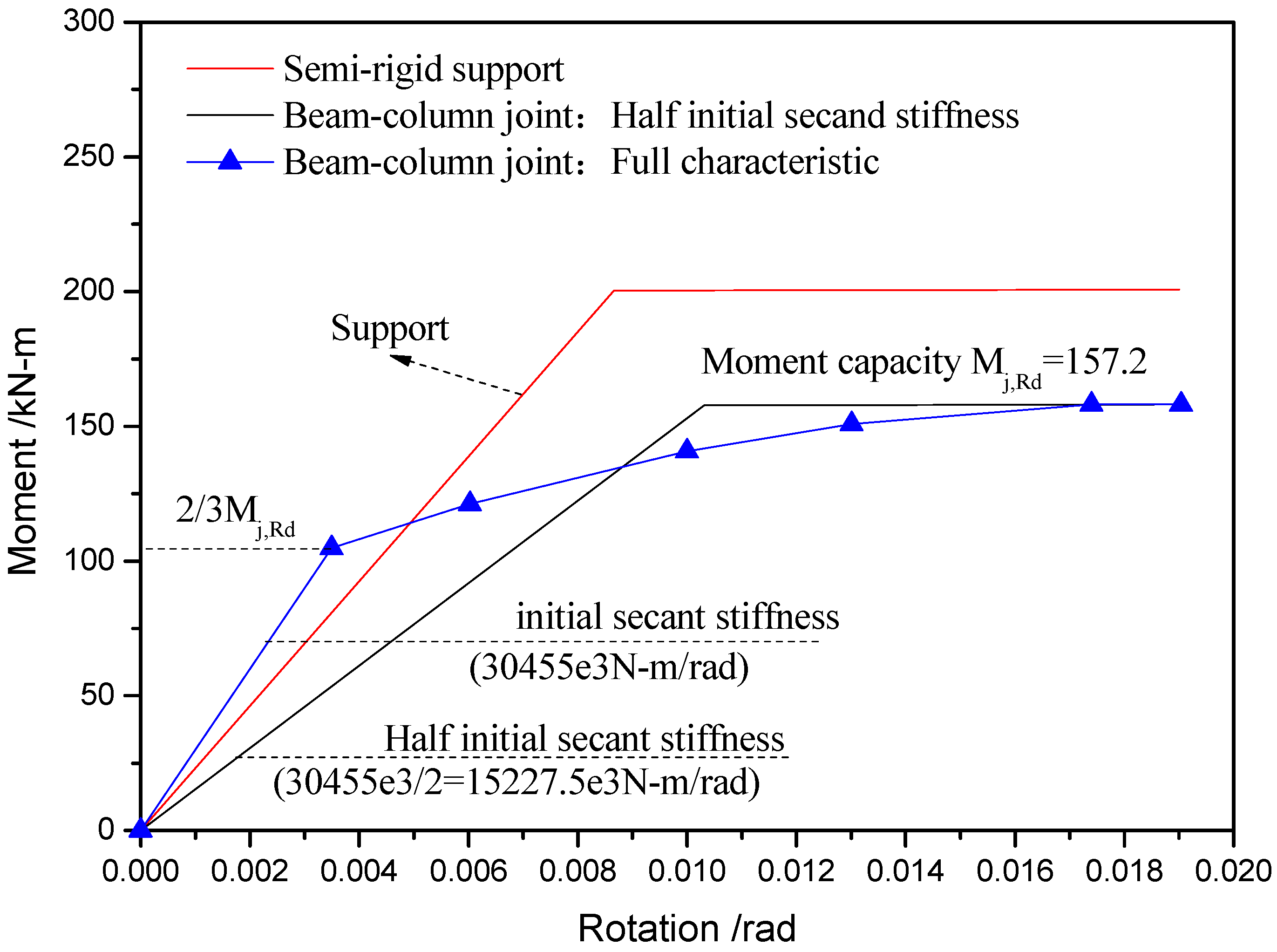
Figure 15.
Displacement response on the top of the steel frame.
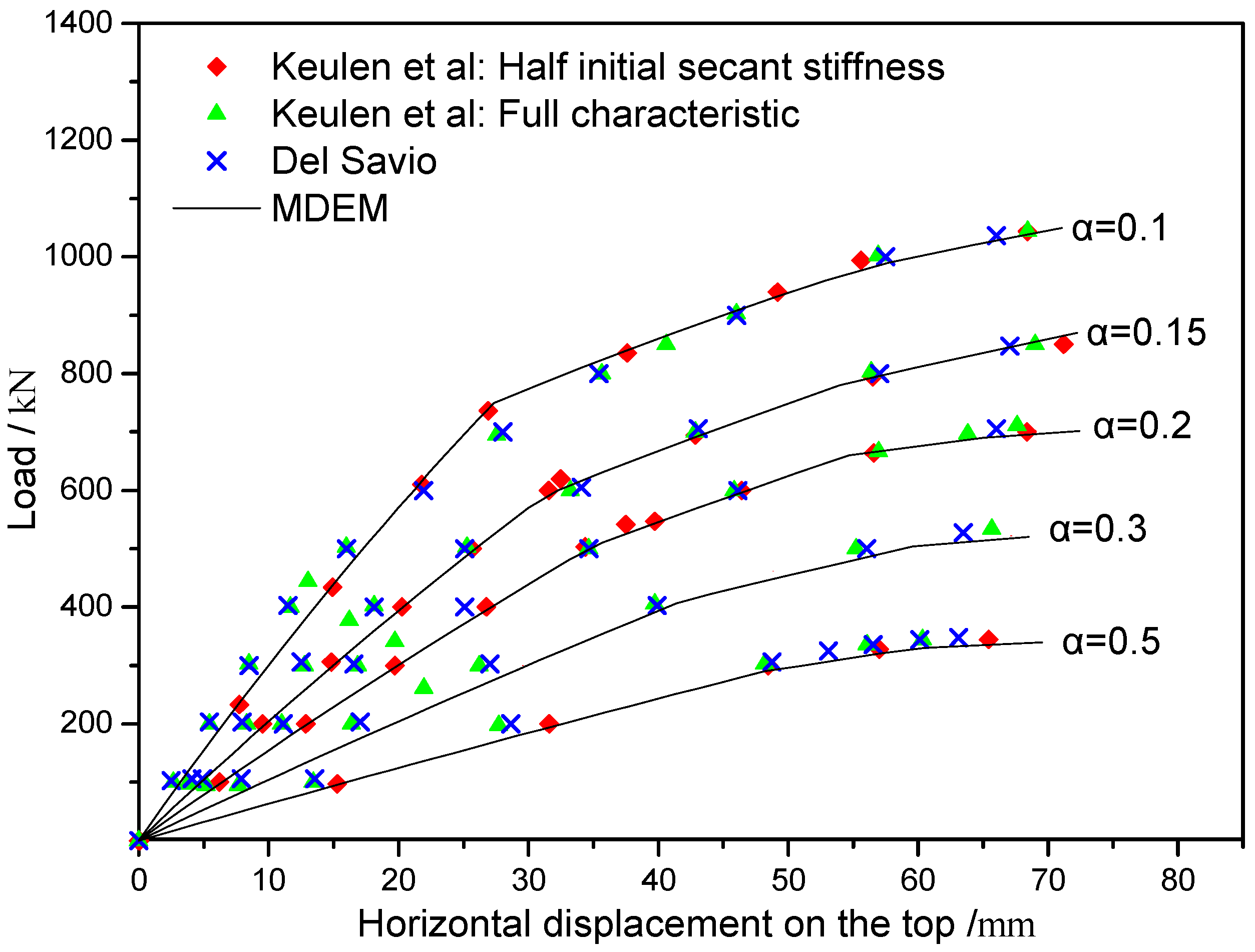
Figure 16.
Load-moment curves of joints and supports.
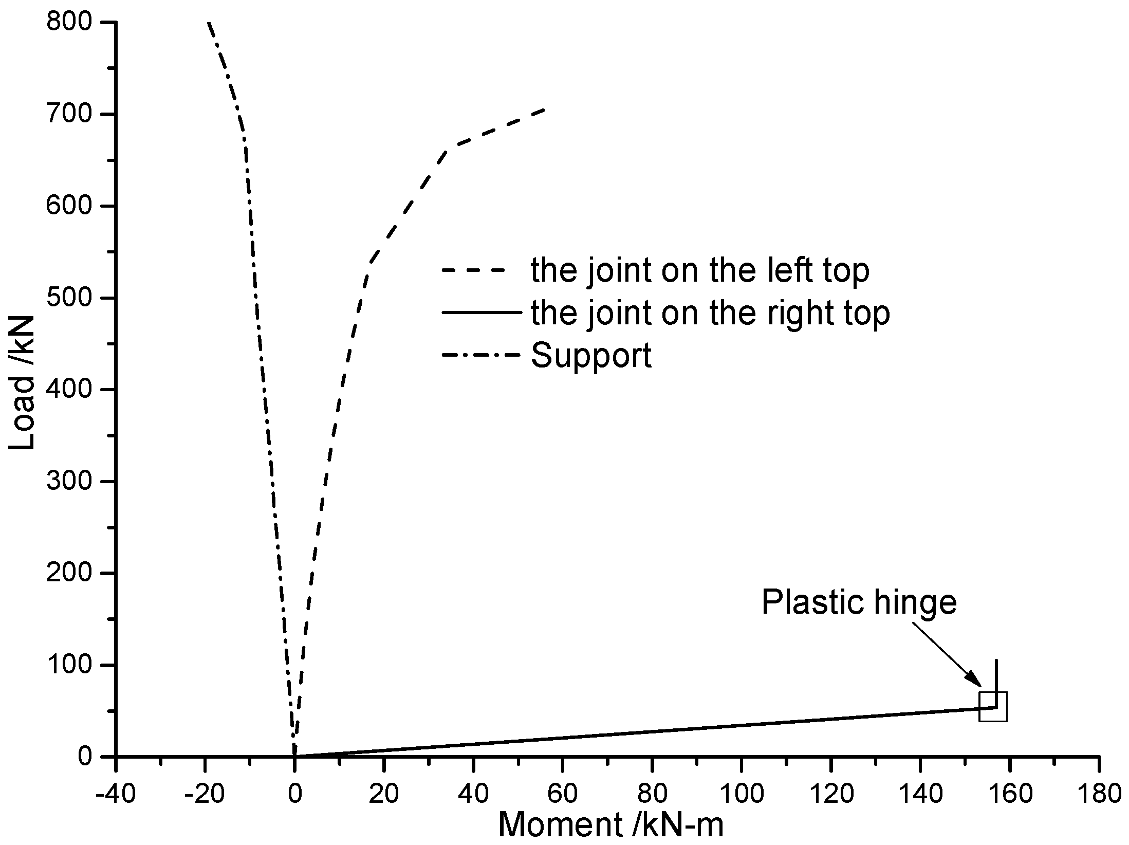
Figure 17.
A single-span three-story steel portal frame with semi-rigid connections and supports.

Figure 18.
Load-moment curves.
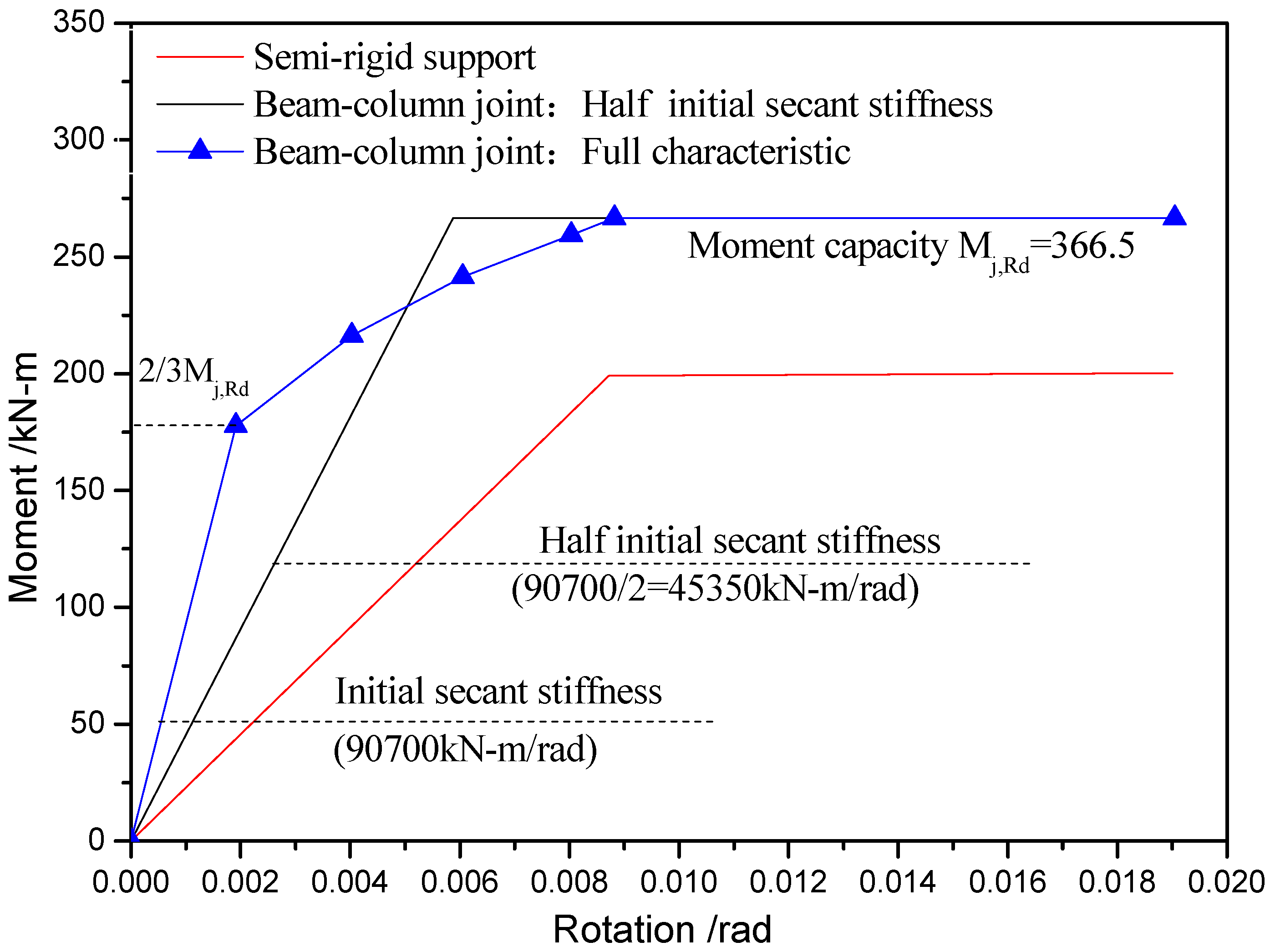
Figure 19.
Load-Displacement curves at each floor of the steel frame.
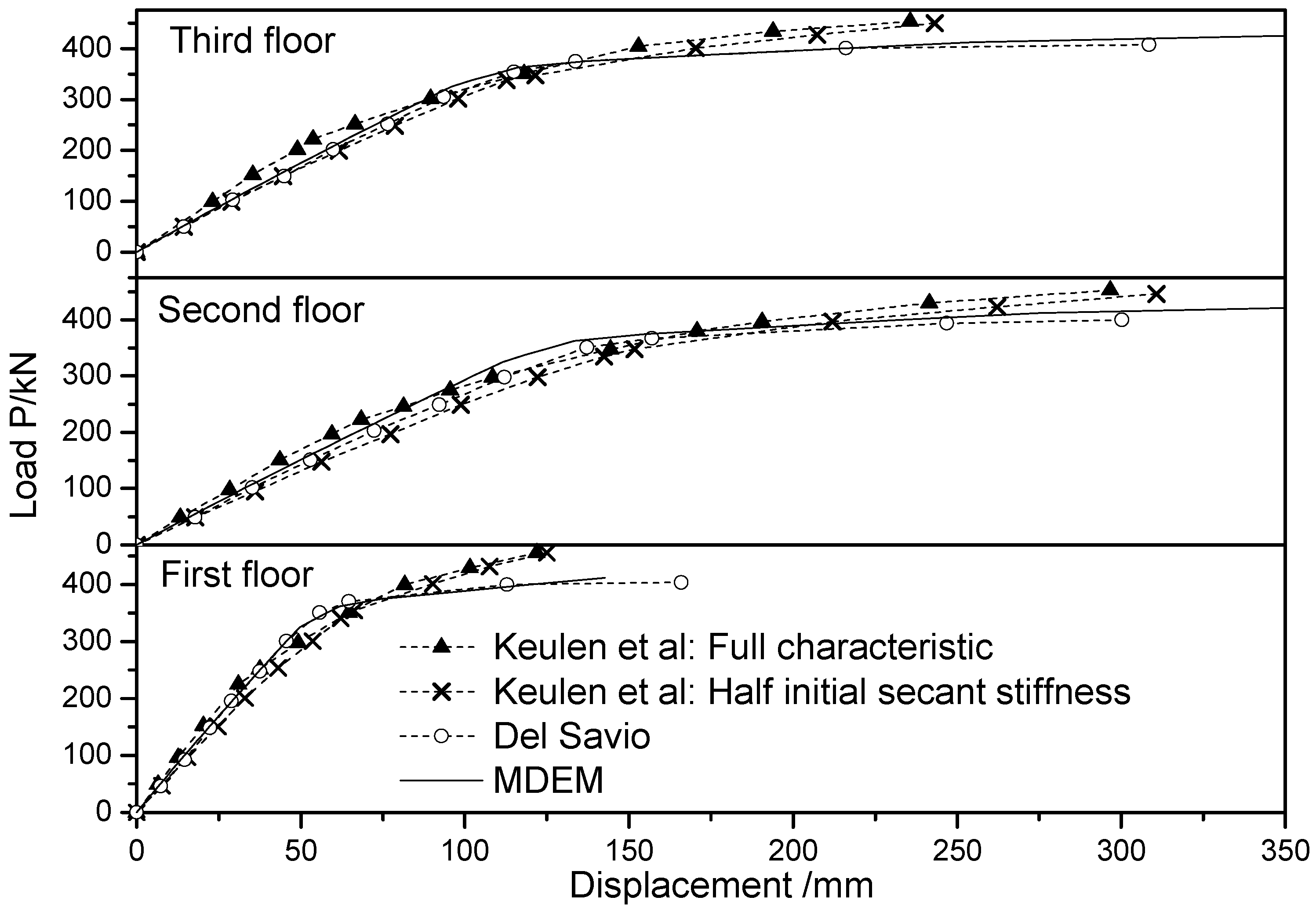
Figure 20.
Load-Moment curves at the right joints and support.

Figure 21.
Configuration and loading of the two-span, six-story Vogel steel frame.

Figure 22.
Horizontal displacement response of the top joint.

Figure 23.
Hysteresis loops at the semi-rigid connection G.
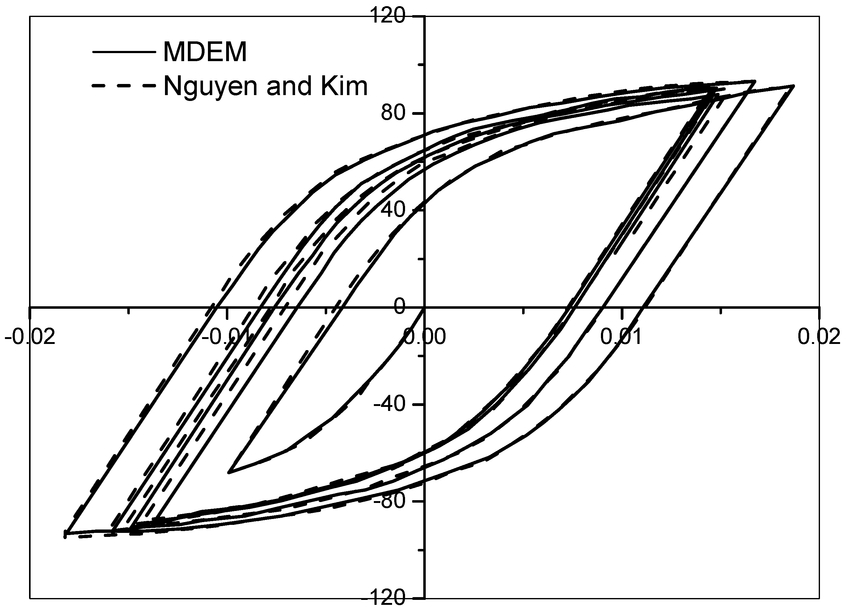
Figure 24.
Failure processes of the steel frame with rigid connection.
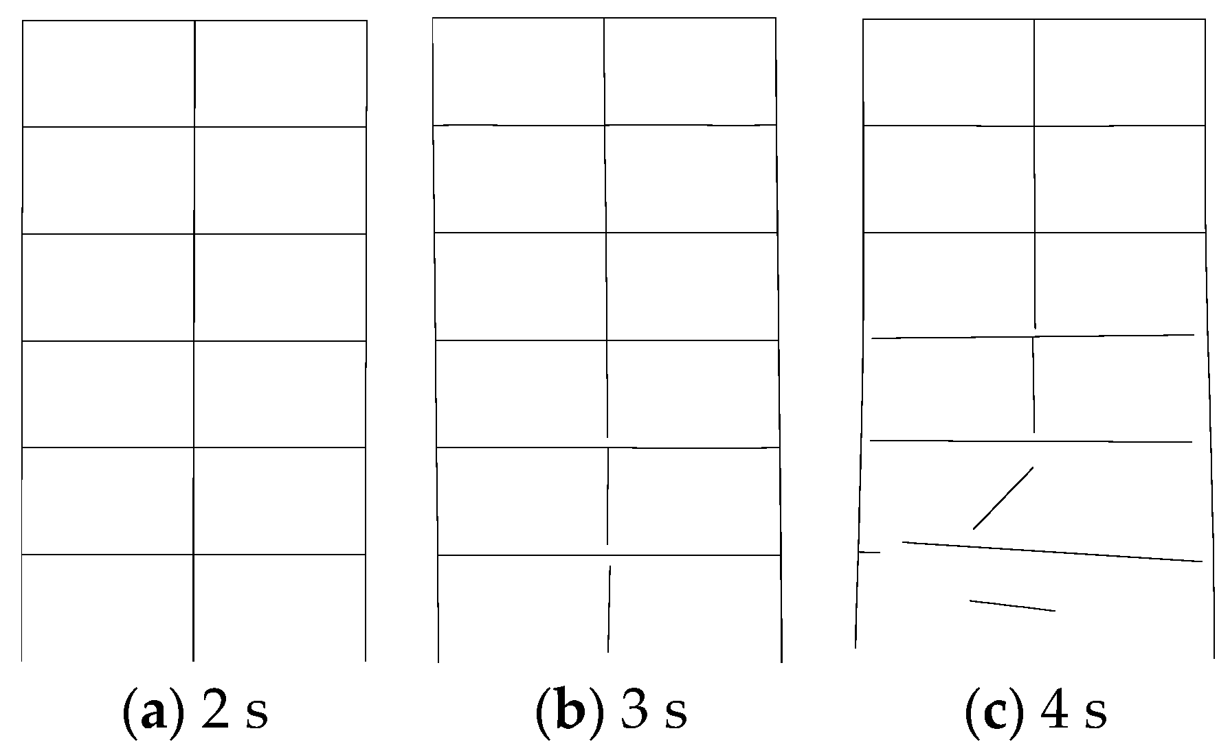
Figure 25.
Failure processes of the steel frame with semi-rigid connection.


Table 1.
Specific formulas for modifying rotational stiffness for three semi-rigid connection types.
Table 1.
Specific formulas for modifying rotational stiffness for three semi-rigid connection types.
| Semi-Rigid Connection Types | Configuration | Formulas |
|---|---|---|
| Elastic support |  | |
| Couple-bar joint |  | (for two same bars) |
| Beam-column joint |  | (for semi-rigid connections on the beam) |
© 2017 by the authors. Licensee MDPI, Basel, Switzerland. This article is an open access article distributed under the terms and conditions of the Creative Commons Attribution (CC BY) license (http://creativecommons.org/licenses/by/4.0/).
Share and Cite
MDPI and ACS Style
Ye, J.; Xu, L. Member Discrete Element Method for Static and Dynamic Responses Analysis of Steel Frames with Semi-Rigid Joints. Appl. Sci. 2017, 7, 714. https://doi.org/10.3390/app7070714
AMA Style
Ye J, Xu L. Member Discrete Element Method for Static and Dynamic Responses Analysis of Steel Frames with Semi-Rigid Joints. Applied Sciences. 2017; 7(7):714. https://doi.org/10.3390/app7070714
Chicago/Turabian StyleYe, Jihong, and Lingling Xu. 2017. "Member Discrete Element Method for Static and Dynamic Responses Analysis of Steel Frames with Semi-Rigid Joints" Applied Sciences 7, no. 7: 714. https://doi.org/10.3390/app7070714
Note that from the first issue of 2016, this journal uses article numbers instead of page numbers. See further details here.