Article

A Neural Networks Approach for Improving the Accuracy of Multi-Criteria Recommender Systems

by
Mohammed Hassan
*,† and
Mohamed Hamada
Software Engineering Lab, Graduate School of Computer Science and Engineering, University of Aizu, Aizuwakamatsu-city 965-8580, Japan
*
Author to whom correspondence should be addressed.
These authors contributed equally to this work.
Appl. Sci. 2017, 7(9), 868; https://doi.org/10.3390/app7090868
Submission received: 28 July 2017 / Revised: 15 August 2017 / Accepted: 16 August 2017 / Published: 25 August 2017

Abstract

:
Accuracy improvement has been one of the most outstanding issues in the recommender systems research community. Recently, multi-criteria recommender systems that use multiple criteria ratings to estimate overall rating have been receiving considerable attention within the recommender systems research domain. This paper proposes a neural network model for improving the prediction accuracy of multi-criteria recommender systems. The neural network was trained using simulated annealing algorithms and integrated with two samples of single-rating recommender systems. The paper presents the experimental results for each of the two single-rating techniques together with their corresponding neural network-based models. To analyze the performance of the approach, we carried out a comparative analysis of the performance of each single rating-based technique and the proposed multi-criteria model. The experimental findings revealed that the proposed models have by far outperformed the existing techniques.

1. Introduction

Recommender systems (RSs) are software tools that have been widely used to predict users’ preferences and recommend useful items that might be interesting to them. The rapid growth of online services such as e-commerce, e-learning, e-government, along with others, in conjunction with the large volume of items in their databases makes RSs become important instruments for recommending interesting items that are not yet seen by users. RSs are usually categorized based on either the techniques used to make the recommendation or the kind of services they provide to users. Various techniques have been explored to develop RSs. The most commonly used techniques are collaborative filtering, content-based, knowledge-based, and hybrid-based techniques [1,2]. Each of these techniques has been applied in many RS applications, and they have worked with considerable success. However, research has shown that these traditional recommendation techniques have their shortcomings, such as sparsity and cold start problem, overspecialization, and so on [3,4]. More generally, using a single rating to make predictions is considered by the recommender systems research community as one of their great limitations [5]. Because the acceptability of the item recommended to the user may depend on many utility-related attributes that the user might take into consideration when choosing the item.
Multi-criteria recommendation techniques extend the traditional approaches by increasing the number of ratings to cover various attributes of the items and incorporate their ratings for improving the prediction accuracy of the RSs. The criteria are the different attributes of items that can be put together to describe the quality of items. For instance, in movie RSs, attributes of movies such as visual effect, direction, story, and action of the movie can affect the choice of a given movie by a user. Some users might prefer movies based on one or more attributes. The multi-criteria technique has been researched and proved to provide higher prediction accuracy than any of the single rating approaches [5]. However, one of the most exciting research directions in multi-criteria RSs is focusing on exploring statistical or machine learning techniques to model the criteria ratings for improving their prediction accuracy. This area is relatively new, and there is much research that has not yet been done extensively. One of the outstanding pieces of research comes in to answer the challenge thrown to the RSs research community by Adomavicius et al. [5] to use more sophisticated machine learning algorithms such as artificial neural networks and aggregation function approaches to analyze the performance of multi-criteria RSs. The same challenge was repeated four years later [5], and to date, no previous research has investigated the performance of multi-criteria RSs using artificial neural networks. Among the initial attempts that explored some of the powerful machine learning techniques is the work Jannach et al. [6], who used support vector regression (SVR) to model the criteria rating. However, using such approaches can be problematic, as working with SVR requires the choice of appropriate hyper parameters that would allow for sufficient generalization of performance, and also as the SVR uses a kernel trick, choosing a suitable kernel function could be a problem as well [7]. This study follows these challenges to use feedforward neural networks trained with a simulated annealing algorithm. Of course, various algorithms like gradient-based (e.g., backpropagation and Levenberg–Marquardt algorithms), genetic algorithms, and so on can be used to train feedforward networks. However, most of these techniques have some weaknesses, such as the tendency to get trapped in local minima, slow convergence rate, long training times, etc. These drawbacks naturally limit the relevance of some of the training algorithms for training neural networks [8]. We chose the simulated annealing algorithm because it has a high tendency to escape local minima, low training times, high convergence rates, and it can deal with chaotic and noisy data [9].
The central questions addressed by this research are: what is the performance level of multi-criteria RSs when modeled by aggregation function approach and using artificial neural networks to predict unknown ratings, and under what circumstances is the better performance achieved? This study has answered the questions by proposing the use of two popular single rating recommendation algorithms (singular value decomposition and slope one algorithms) and comparing their performance with the proposed approach. This paper is composed of five themed sections, including this introduction section. Section 2 gives a brief overview of related background. Section 3 is concerned with the research methodology, and Section 4 presents the results and discussion of our findings. Finally, Section 5 contains the conclusion and future research directions.

2. Related Background

In this section, we briefly introduce the basic concepts of the related topics covered in this paper. The section begins by laying out a short general explanation of RSs and collaborative filtering techniques. Section 2.2 describes the extension of the traditional recommendation technique into multi-criteria recommendations. The remaining two sections contain an overview of artificial neural networks and simulated annealing algorithms, respectively.

2.1. Recommender Systems (RSs)

RSs belong to the subclass of information systems, whose popularity has rapidly increased in recent years. Nowadays, a variety of application domains, such as e-commerce, e-learning, tourism guide, and so on, are using RSs. The aim of RSs is to provide personalized recommendations of online products and services to overcome the growing problems of information overload [10]. They use machine learning algorithms and filtering techniques to predict the opinions of users on items and recommend the most suitable ones among them to the users. Different filtering techniques such as collaborative filtering, demographic filtering, content-based filtering, and hybrid filtering have been widely used to characterize the functions of RSs [11]. Furthermore, recent surveys like the one conducted by Yera and Martinez [12] have enlightened us on the use of fuzzy techniques for supporting RSs. Moreover, as these traditional techniques have some shortcomings, several approaches such as incorporating trust statements into online RSs have been proposed to improve the accuracy of the systems [1,13].

Collaborative Filtering

Collaborative filtering (CF) techniques are the most widely used recommendation techniques that use ratings provided by many users to predict the preferences of the current user and make useful recommendations [13]. The central idea behind CF methods is that they compute similarities between the current user and other users of the systems who previously co-rated some items. The CF techniques are divided into neighborhood-based and model-based techniques. The neighborhood-based methods are sometimes referred to as memory-based. Here, the rating matrices between user–item pairs are stored in in the systems and used directly to estimate ratings for items that are not yet rated by users. The predictions can be made by computing either similarities between users (user-based) or similarities between items (item-based). On the other hand, model-based techniques used machine learning algorithms such as decision tree, Bayesian classifiers, support vector machine, regression model, singular value decomposition, and so on to build predictive models [14]. The rest of this section summarizes the two CF RSs used to undertake our experiments.
  • Singular value decomposition (SVD): SVD is a latent factor model that aims to uncover latent features that determine the observed rating. The field of information retrieval usually applies SVD technique for identifying latent semantic factors. Koren and Bell explained the concept of SVD in [15] using a movie recommendation scenario. Similarly, we studied the Koren SVD [15] and used it to implement a traditional RS. The Koren SVD uses two vectors U and V in I R d with d as the dimension of the latent factor space so that each item i is associated with vector V i and the user u is associated with U u . The resulting dot product V i T U u represents the interaction between u and i. To estimate the final predicted rating of u on i, a baseline predictor that depends on item or user ( r ¯ + b u + b i ) needs to be added to have the relation in (1), where r ¯ is the overall average rating.
    R u i ^ = r ¯ + b u + b i + V i T U u
    The model parameters ( V T , U , b u , and b i ) can be learned by regularized squared error minimization as min V , U , b ( u , i ) S ( R u i r ¯ b u b i V T U ) + η ( b i 2 + b u 2 + V i 2 + U u 2 ) , where S is the set of pairs ( u , i ) for which the ratings of i given by u is known and η is the regularization constant that controls the scope of the regularization and is normally obtained through cross-validation. The well-known popular gradient descent algorithm (GDA) [16] or alternating least squares optimization techniques [17] can typically be used to perform this minimization. Applying stochastic GDA for each rating R u i , the predicted rating R u i ^ is obtained and the relative error ε u i = R u i R u i ^ is measured, then the GDA computes the parameters as:
    V i V i + δ ( ε u i η V i )
    U u U u + δ ( ε u i η U u )
    b i b i + δ ( ε u i η b i )
    b u b u + δ ( ε u i η b u )
    The parameters η and δ can be assigned small positive real numbers such as 0.005 and 0.02, respectively [18].
  • Slope one algorithm: The slope one is a model-based CF algorithm proposed by D. Lemire et al. [19], which was derived from item-based CF technique. It was named slope one algorithm and was proposed to overcome some of the issues encountered in CF-based RSs. Several experiments confirmed its efficiency, and it is easy to implement and maintain, which made it popular and attracted the attentions of the RSs community [20]. It approximates unknown ratings of users on items based on the differences between ratings of the user and those of similar users. In other words, the algorithm uses users who rated the same item or other items rated by the same user. The first of the two steps used for making predictions is to compute the mean deviation of two items as follows. For any two items i j and i k in the training set, slope one algorithm uses (2) to compute the mean deviation M d j k between them, where r u j r u k is the difference between ratings of i j and i k by the same user u and | U j k ( S ) | 0 is the number of users who rated i j and i k , and S is the set of all users. The target rating r v j ^ of the user v on item j will be obtained finally from (3), where r v c is the rating of v to other items c, and the total number of the user’s ratings | r v c | 0 . The recommendation follows the top-N technique.
    M d j k = u U j k ( S ) r u j r u k | U j k ( S ) |
    r v j ^ = 1 | r v c | c ( r v c + M d j c )

2.2. Multi-Criteria Recommender Systems (MCRSs)

Traditionally, RSs solve recommendation problems by assuming that there exist two sets: Users and Items, representing the set of all users of the system and the set of all prospective items that can be recommended to users, respectively. Their utility functions f: Users × Items → r measure the likelihood of recommending items to users. The users’ preferences given by r take a real number ( r I R ) within some interval (e.g., between 1 and 5, 1 and 10, etc.) in some cases. Therefore, the main goal of the system is ∀uUsers to estimate the function f(u, i, r) for which r on iItems for u is not yet known, and to recommend i’s according to the strength of their r [5].
In traditional RSs, f(u, i, r) estimates an overall rating r o defined as f: u × i r o . However, utility functions of MCRSs extend that of traditional techniques by increasing the number of ratings from 1 to n ( r 1 , r 2 , . . ., r n ), covering n attributes of the items. This could assist in enhancing the recommendation accuracy since more complex user preferences could be represented by multiple criteria ratings (see (4)).
f ( u , i ) r o × r 1 × r 2 × r 3 × × r n
Considering the difference between traditional RSs and MCRSs, additional techniques are required to integrate the criteria ratings when developing the systems. Different approaches have been proposed to estimate ρ i for i = 1 , 2 , , n , and these modeled to predict the value of ρ o that represents the preferences of the user. Heuristic-based and model-based approaches are commonly adopted methods in many of the MCRS studies [5]. For this study, we explored the model-based approach because of its several advantages over heuristic-based approaches. For instance, unlike the heuristic-based approach, which can only work with similarity-based traditional collaborative filtering techniques, the model-based approach can work with any traditional technique. The model-based approach determines the unknown r i and the value of r o by building a predictive model that learns from the observed data. These predictive models include the probabilistic modeling approach, support vector regression approach, and an aggregation function approach which assumes r o to be an aggregation of r i , as shown in (5). Among all these models, the aggregation function model is the most widely used because it has the potential to work with several machine learning techniques (e.g., artificial neural networks) to more accurately estimate user preferences.
r o = f ( r 1 , r 2 , r 3 , , r n )
Let k m be a criterion for m = 1 , 2 , , n . The following steps summarize the aggregation function approach for n criteria recommendation problems:
  • Decompose the multi-criteria rating problem into single-rating problems.
  • For each k m , use a single-rating technique to predict unknown rating r i for each criterion separately.
  • Learn the relationship between r o and r i s using the selected algorithms, such as artificial neural networks.
  • Integrate steps 2 and 3 to predict r o for r 1 , r 2 , , r n .

2.3. Artificial Neural Networks (ANNs)

In 1943, McCulloch and Pitts published a paper [21] in which they introduced the first model of an A N N [22] based on a single-layer neural network. The A N N is a powerful class of machine learning algorithms that learn complicated patterns from data using collections of simple trainable mathematical functions. While a variety of definitions of A N N s have been suggested, this paper follows the definition given by the inventor of one of the first neuro-computers [23] in 1989, who saw it as “a computing system made up of a number of simple, highly interconnected processing elements, which process information by their dynamic state response to external inputs”.
A N N s mimic the structure of the human brain, which consists of several processing units called neurons. They are made up of two or more interconnected layers of neurons that take inputs from the external environment through an input layer and send the results to the external environment through an output layer as an output. In most cases, the input layer is connected to a hidden layer(s) that is/are between the input and output layers. Neurons between layers are connected using a system of weighted connections similar to synapses in the biological human brain.

2.4. Simulated Annealing Algorithm (SMA)

S M A is an optimization algorithm similar to the method of material physics for cooling substances like metal from a high energy level to a lower level. Training A N N s with the S M A started as far back as 1994, when Goffe et al. [24] tested the performance of SMA-based networks on four econometric problems, and compared the results with the simplex, quasi-newton, and conjugate gradient-based networks. The S M A -based network was found to outperform the networks trained with the other training algorithms [25]. However, the efficiency of S M A over the usual gradient descent-based backpropagation algorithm was not confirmed until five later, when Sexton et al. [25] researched to investigate and compare the performance of the backpropagation algorithm with global search algorithms, and S M A was found to be the superior training algorithm for A N N s .
The technique used in this study to implement and train the S M A -based network is similar to that of [24,25]. The summary of the process is as follows: Let W be a vector of weights ω i , and E(W) be the error function that computes the errors produced by the current elements of W, and let V be the matrix of step length of W. E(W) is evaluated with the current weights in W, and the next weights vector W will be calculated for each i by varying its ω i using (6), where v i V , and r is a randomly generated real number between −1 and 1.
ω i = ω i + r v i
Accepting the W instead of the current W will be decided based on the errors E( W ) and E(W), respectively. If E( W ) is smaller than E(W), then W is accepted directly as the current weights matrix. Otherwise, the Metropolis [26] algorithm will be applied to test the likelihood of acceptance or rejection. If the probability of acceptance is high, W will be accepted, and W will be saved together with E(W) to prevent loss of the better solution. The starting temperature will be reduced to T (see (7)), and k is randomly generated between 0 and 1 exclusive.
T = T k
The process continues until the stopping conditions such as the target error or the experiment reach the maximum number of training circles.

3. Experimental Methodology

This section presents the summary of how the research was carried out by discussing the experimental framework of our proposed method together with how the system was modeled. To begin with, the following subsection gives the detailed analysis of the datasets used to conduct the experiments, and Section 3.2 explains the mechanism used to build the proposed MCRSs.

3.1. Analysis of the Dataset

The experiments were conducted using two multi-criteria datasets from two different domains.

3.1.1. Yahoo!Movie dataset

The Yahoo!movie dataset: It is a multi-criteria dataset where preference information on movies was provided by users on the strength of four different movie attributes (criteria); namely, the direction ( k 1 ), the action ( k 2 ), the story ( k 3 ), and the visual ( k 4 ) effect of the movie [27]. Ratings of each criterion were measured on a 13-fold scale starting from F representing the lowest preference to A + , which stands for the highest preference. In addition to the criteria ratings, an overall ( k o ) rating that measures the final acceptability of users on movies was also included in the dataset. Table 1 displays the sample of the dataset used in the first experiment. The table is divided into two parts, containing the form of the dataset extracted directly from Yahoo!Movies website in the first part.
However, for the model to process the data easily, the rating scale was transformed into a numerical rating by changing F to 1 and A + to 13 to represent the lowest and highest preference values, respectively. The second part of the table contains the transformed data equivalent to that in the first part.
Furthermore, to detect and remove inconsistencies from the dataset to improve its quality, the dataset was cleaned to eliminate cases of missing ratings for at least one of the four criteria and the overall ratings. Moreover, to ensure an adequate set of evaluated items for each user, the cleaning process was again applied to remove users who rated less than five movies. At the end, the dataset contained a total of 6078 users and 976 movies which give a total of 62,156 ratings in the dataset. Nevertheless, to analyze the frequency of each rating value (1 through 13), the dataset was divided into five separate portions (the four criteria and the overall) containing UserID, ItemID, Value, for each criterion and the overall rating. Table 2 gives the basic statistics of the rating values by computing the number of times each value appears in the dataset, the approximate percentage, and cumulative percentage rounded to the nearest whole numbers. Though the tables for similar statistics for the other four criteria are not presented in this paper, the same approach was followed to analyze all of them. The average rating for the direction, the action, the story, the visual, and the overall ratings in three decimal points are 9.534 , 9.567 , 9.900 , 10.092 , and 9.522 respectively.

3.1.2. TripAdvisor Dataset

The hotel rating dataset: The second experiment was carried out using a hotel booking dataset extracted from TripAdvisor (https://www.tripadvisor.com/), for recommending hotels to users based on six aspects (attributes) of the hotels. In addition to the Overall rating, the dataset contains Value aspect rating, Rooms aspect rating, Location aspect rating, Cleanliness aspect rating, Check in/front desk aspect rating, and Business Service aspect rating [28]. The ratings are presented on a scale of 7, ranging from 0 to 5 stars, and −1 indicates this aspect rating is missing in the original dataset. Table 3 shows the sample of the TripAdvisor dataset. The dataset contains 246,098 ratings of 148,183 users on 1851 hotels. In addition to rating information, the dataset initially contained supplementary information such as the date, contents, etc. To obtain the data in Table 3, we performed data cleaning to remove the unwanted entries and all cases of having only the users’ and hotels’ IDs without giving ratings to at least one aspect. Users with low counts were also excluded to reduce the costs of experimentation.
Furthermore, we conducted basic statistics of the dataset to show the strength of correlations between ratings of the six aspects and the overall ratings. Table 4 presents the approximation of the correlations between criteria (aspect) ratings and the overall rating. Although the statistical analysis of the table revealed that all the aspect ratings had positive correlations with the overall ratings, it can be seen from the table that the location aspect has the highest influence in deciding the overall ratings. However, the table also illustrates that the business service of the hotels had the least significance in computing the overall ratings, compared to the other aspects. Column three of this table contains the approximate correlations between the overall ratings and criteria ratings.

3.2. Systems Implementations and Evaluations

In this section, the framework of the proposed model is summarized (Section 3.2.1) and details of the implementation of the systems are discussed (Section 3.2.2). Finally, Section 3.2.3 explains the evaluation metrics used in assessing the accuracy of the systems.

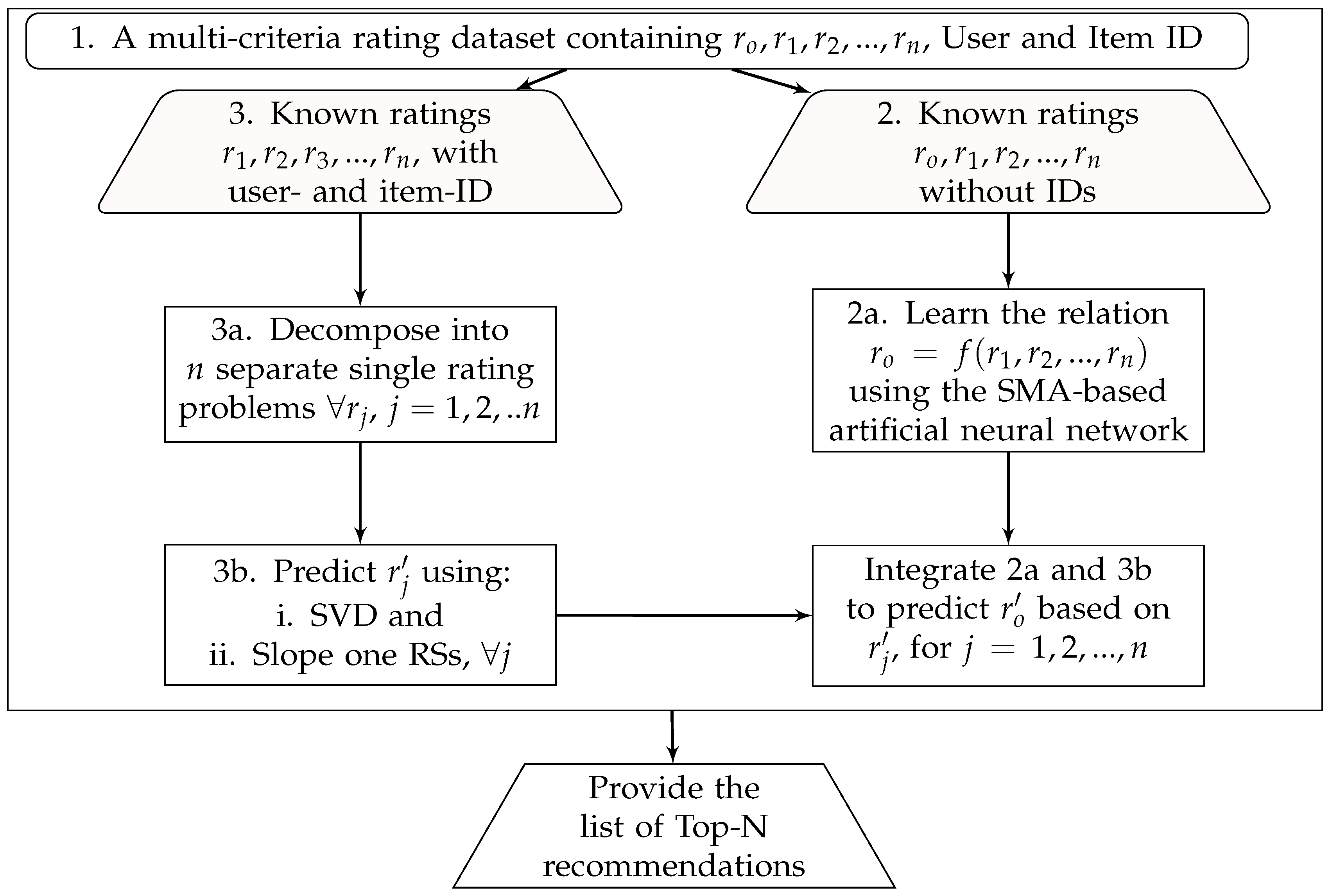
3.2.1. The Proposed MCRSs Framework

Building MCRSs using an aggregation function approach requires three-to-four important steps, as enumerated in Section 2.2 when discussing MCRSs. It starts by decomposing the n-dimensional rating problem into n single-rating problems, followed by choosing the preferred aggregation function that can work on n-dimensional ratings to finally estimate the overall rating. This process combines the proposed aggregation function with a traditional recommendation technique that can compute individual criteria ratings to be used for the prediction of the overall ratings. Figure 1 summarizes the basic idea behind the proposed technique and the steps required to provide top-N recommendations.
As can be seen from the figure, the model starts by loading the multi-criteria dataset and dividing it into two parts. One part contains only the ratings ( r o to r n shown in step 2) to train the SMA-based neural network for learning the relationship between the criteria ratings and the r o given in (5) at page 4. However, this part did not require the user- and item-ID. The data in step 3 contains the criteria ratings ( r 1 , r 2 , r 3 , , r n ), user-ID, and item-ID to learn the behavior of users relative to each attribute of the items. Here, the overall rating is not needed. Similarly, The two traditional techniques (SVD and slope one) learn and predict the criteria ratings for new items. Finally, the model predicts the overall rating for new items by integrating the trained neural network and the single rating technique. Top N items will be recommended to the user based on the strength of the corresponding r o of the items.
Therefore, following the architectural framework presented in Figure 1, the three models implemented and used to conduct the experiments are enumerated below.
  • An ANN was implemented and trained using SMA and the datasets to learn the relationship between the criteria ratings and the overall rating.
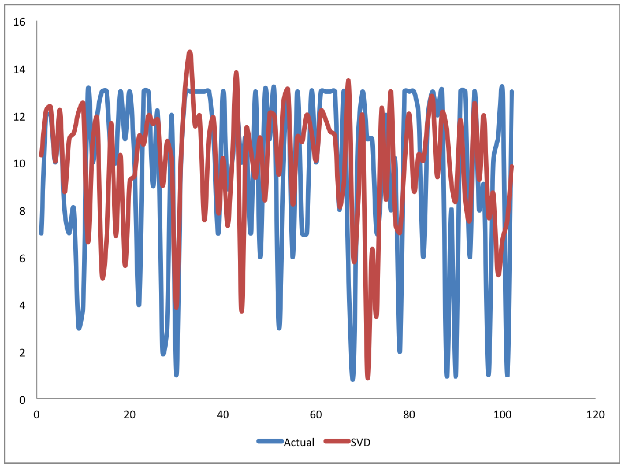
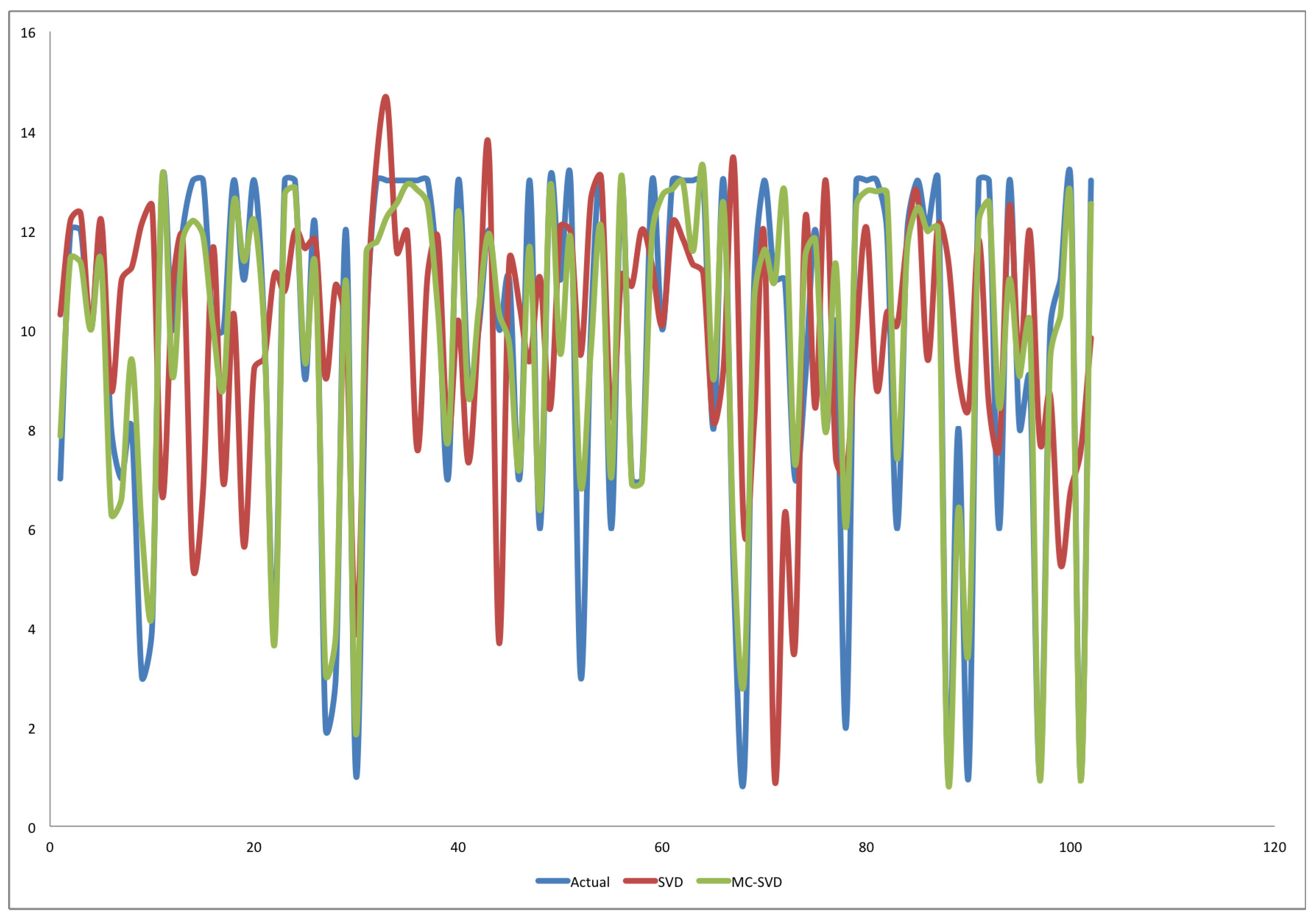
  • Two traditional RSs were built using two different techniques (slope one and SVD); each of them can learn and predict the decomposed n-dimensional ratings separately from the dataset.
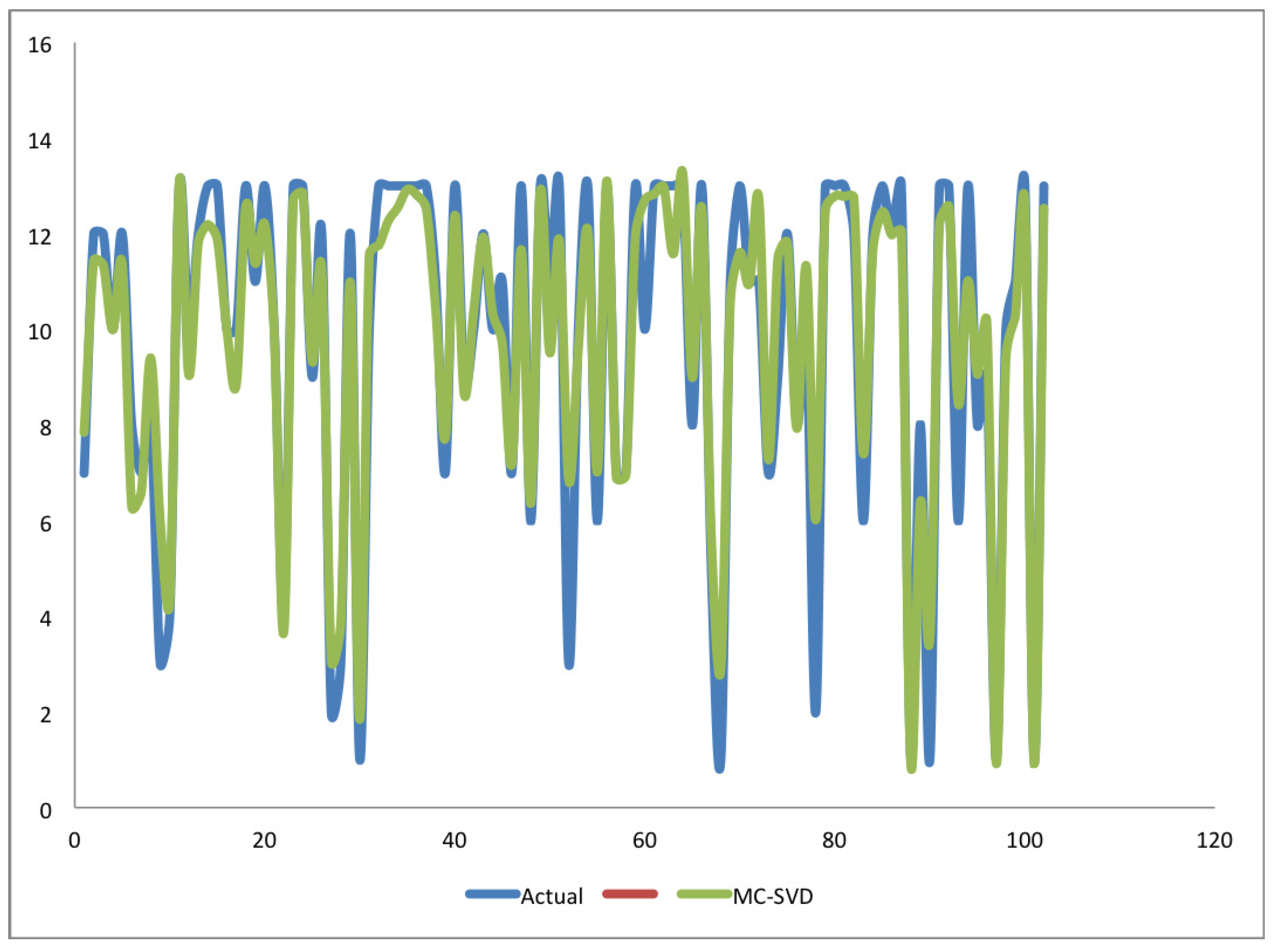
  • Two MCRSs have been developed by integrating the SMA-based networks with the two traditional techniques separately.

3.2.2. Implementation

Java was chosen as the programming language to implement all the systems used for this study. The choice of the programming language follows several books [29] and papers [30] that we consulted and obtained hints on how to implement the system in Java.
RSs are complex software tools that gather many interacting components, starting from loading the data into the memory, down to presenting the results to the users after performing some internal computations. Their design and implementation entail understanding the type of users and the type of data available to describe the items. The explanations given here may not be sufficient for a beginner to learn the techniques for designing RSs, but the references above and the work of Picault et al. [31] could give the required skills on how to get RSs out of the lab.
Nonetheless, regardless of the methods and techniques used to build RSs for research purposes, the systems need to be evaluated experimentally using at least one of the following evaluation techniques. The offline experiments: which require no mutual interaction with the real users. The second evaluation method is the user study: where a group of users will be asked to use the system in a particular controlled environment and give their feelings about the system. Thirdly, the systems can be evaluated when used by many real users over an extended period, normally without prior thinking of the experiment [32].
To evaluate our proposed systems, we followed offline experiments to simulate the interactions of real users with the real systems, where the systems will predict the user preferences and make recommendations. The users will then make corrections on the predictions of the systems and check whether the recommendations made by the systems are useful. This interaction was simulated by recording the interactions of users and the systems using datasets and hiding some of the interactions (called test data) to practice how users would rate some items and what will be the acceptability of the recommendations done by the systems.
There are several general rules for how the test data could be selected. These include the Pareto principle [33], cross-validation [34], held-out method [35], and so on. Cross-validation is one of the popular ways of selecting the test data, where the dataset will be split into some equal partitions, and every partition will be used in turn as the test data. We chose cross-validation so that more data in the ranking algorithm will be used, and the effect of variation in the training set will be taken into consideration [32].

3.2.3. Evaluation Metrics

Moreover, to evaluate the accuracy of the systems, we used three main methods of measuring prediction accuracy, as follows:
  • Rating prediction accuracy: Root mean square error ( R M S E ) in Equation (8) and mean average error ( M A E ) in Equation (9) were used to measure rating prediction accuracy, where | N t | is the number of test sets, r u i ^ and r u i are the predicted and actual ratings from the test set, respectively.
    R M S E = 1 | N t | ( u , i ) N t ( r u i ^ r u i ) 2
    M A E = 1 | N t | ( u , i ) N t | r u i ^ r u i |
  • Usage prediction: A P r e c i s i o n which measures the segment of useful recommendations among those predicted as useful by the systems (Equation (10)). A R e c a l l , which is defined in a standard way by Adomavicius et al. [36] as a metric for estimating part of useful recommendations out of all the items acknowledged to be useful (Equation (11)). F- m e a s u r e , which served as a harmonic mean of the precision and recall (Equation (12)), which are the most useful measures of interest for some number of recommendations were used in measuring usage predictions. In Equations (11) and (12), the term # t p means the number of true positive, which indicates the number of useful predictions. The # f n stands for the number of useful predictions that are not among the top-N recommendation list, and # f p is the number of false positive that represents the total number of non-useful predictions.
    P r e c i s i o n = # t p # t p + # f p
    R e c a l l = # t p # t p + # f n
    F m e a s u r e = 2 P r e c i s i o n × R e c a l l P r e c i s i o n + R e c a l l
  • Ranking accuracy: We used three evaluation metrics for measuring the ranking accuracy of RSs to evaluate the systems. The area under the curve ( A U C ) of a receiver operating characteristics ( R O C ) curve in Equation (13) for each user u, which measures how accurate the algorithms’ separate predictions into relevant and irrelevant by finding the area under the curve of the sensitivity rate (recall) against the specificity. The r a n k u k + is the position of the kth relevant item among the N recommended items.
    A U C u = 1 N i = 1 # t p u r a n k u i + + # t p u + 1 2
    The second ranking metric is the normalized discounted cumulative gain ( N D C G ), which is a ratio between the discounted cumulative gain ( D C G ) and the ideal D C G ( I D C G ) (see Equation (14)) that also measures the performance of RSs based on the graded relevance of the recommended entities. The D C G shows the correctness of the ranking. It takes a real number between 0 and 1, and the larger the D C G , the better the ranking accuracy of the algorithm. The I D C G is the maximum D C G value for a given set of queries. The r e l k in the equation takes 1 if the item at position k is relevant, and 0 otherwise.
    N D C G = D C G I D C G = r e l 1 + 2 N r e l k l o g 2 k r e l 1 + 2 # t p u 1 r e l k l o g 2 k
    Similarly, the fraction of concordant pairs ( F C P ) in Equation (15) was also used to ensure the correct measurement of the ranking accuracy. The n c represents the number of concordant pairs defined as n c = u U | ( i , j ) | { r ^ u i > r ^ u j r u i > r u j } , and n d is the corresponding number of discordant pairs calculated as n d = u U | ( i , j ) | { r ^ u i > r ^ u j r u i r u j } . This means that the concordant pairs are predicted ratings r ^ u i and r ^ u j for some items i and j so that if r ^ u i > r ^ u j , then their corresponding ratings r u i and r u j from the dataset must satisfy the same condition r u i > r u j ; otherwise, the items i and j are called discordant pairs.
    F C P = n c n c + n d
The percentage correlations between predicted ratings and the actual ratings were calculated using Pearson correlation coefficient to establish how close the predicted ratings of each of the techniques are to the real ratings from the dataset.

4. Results and Discussion

To compare the proposed M C R S s approaches with the traditional single rating techniques, we performed two separate experiments based on the domains of the extracted datasets. Therefore, this section is subdivided into two subsections, and each subsection gives a summary of the experimental findings.

4.1. Experiment One

Experiment one was conducted using the Yahoo!Movie dataset, and it was carried out five times by changing the global recommendation settings, which include N-fold cross-validation with different values of N for splitting the dataset into training and test sets, and t o p N that was used by precision and recall so as to find out under what circumstances (values of N and N) the proposed aggregation function-based MCRSs would provide better performance accuracy compared to their corresponding single-rating traditional approaches. The experiments were divided into five stages with different N N values as 10–10, 5–10, 10–5, 5–5, and 5–4, where each case stands for N f o l d t o p N general settings. The N f o l d cross-validation breaks the dataset into N sets of approximately the same size. N 1 sets are to be used for training, and the remaining set as a test set. This process will be repeated N times, and the model provides the mean accuracy of each metric.
Although any single rating recommendation technique could be used to perform similar experiments, we decided to use matrix factorization S V D and the slope one algorithm, whose better prediction accuracy have been established by various studies in RSs [6]. As mentioned in Section 3.2, we used M A E , R M S E , p r e c i s i o n , r e c a l l , F- m e a s u r e , A U C , N D C G , and F C P to investigate and analyze the predictive performance of all four techniques. They are named as S V D to represents the matrix factorization S V D , S l o p e O n e for the slope one algorithm, M C - S V D for the proposed M C R S s that worked with the S V D , and M C - S l o p e for M C R S s that worked alongside the S l o p e O n e technique. The outcomes of evaluating their predictive performance are presented in Table 5. The last part of the table contains the average of each metric from the five categories of the experiments, which show the improved accuracy of our proposed A N N -based models.
The resulting R M S E , M A E , A U C , and F C P presented in Table 5 confirmed that the proposed aggregation function model integrated with S M A -based networks are by far more accurate than their corresponding traditional single rating algorithms. Interestingly, even the M A E that does not deal with larger errors as well as the R M S E metric, the proposed techniques show greater accuracy in all the experiments than the single-rating-based techniques.
Table 6 and Table 7 report the numerical differences in accuracies between the two A N N -based models and the single rating techniques. The tables have shown the decrease in R M S E and M A E and also increase in F- m e a s u r e A U C , N D C G , and F C P , that highlight the positive performance of A N N -based MCRSs. The experimental results showed clear accuracy improvements over the ones observed in earlier studies [6,27,37].
Furthermore, to emphasize the good performance of our models, we conducted some statistical analysis by extracting some of the predicted ratings of all the algorithms and comparing them with the actual ratings from the dataset. Table 8 contains the percentage correlations between the actual and predicted values for each of the four experimented techniques. As we have already seen when giving the basic statistics of the dataset in Table 2, the minimum and maximum ratings in the dataset are 1 and 13, respectively. We also found the corresponding minimum and maximum values from the predicted values of each of the techniques, and the result is also included in Table 8. However, the table gives only numerical values to show the strength of the relationships that exist between the predicted ratings and actual ratings. For instance, if there exist some deviations or outliers between the ratings, the correlation in the table did not show the real behavior of each technique. It is therefore important to further analyze the monotonic relationship between them. Figure 2, Figure 3 and Figure 4 are graphs of actual vs. M C - S V D , actual vs. S V D , and actual vs. the two techniques ( M C - S V D and S V D ), respectively. Figure 4 shows several errors from single-rating S V D , where in many instances it did not move in line with actual values from the dataset. It is apparent from the data in Figure 2 that most of the predictions of the single-rating S V D are not even close to actual ratings. Strong evidence of these inconsistencies can be observed in several places on the figure. For example, it predicted lower ratings such as 4, 2, and 1 as 11, 9, and 3 respectively. Other surprising predictions observed from the graph are several occasions where S V D could not accurately predict high ratings; it either predicted them to be higher than the actual or in most cases, it predicted the ratings to be between 6 and 12. Turning now to Figure 3, it can be seen that it is not surprising that in Table 5 through Table 8 the M C - S V D had better performance than all the single-rating techniques. The figure shows significant correlations between the two curves. Moreover, comparing the three curves in Figure 4, we can further see that the same ratings by S V D as approximately 11, 9, and 3, instead of 4, 2, and 1, the M C - S V D approximates them as 4, 3, and 3, respectively. The predictions of M C - S V D are almost similar to the actual values. Although the M C - S V D is not always giving the correct predictions, even its incorrect predictions are much better than that of the single-rating S V D .
Together, these results indicate that modeling MCRSs with artificial neural networks significantly improved the accuracy of the systems.

4.2. Experiment Two

This experiment was conducted to evaluate potential biases by re-evaluating the proposed approach with another dataset from a different domain (hotel rating dataset). We followed similar methods to the ones applied in the previous experiment. However, in addition to the changes in the dataset used for the two experiments, small changes have been made by increasing the number of the network’s neurons to account for the two additional criteria ratings. Furthermore, since no single situation was reported among the five experiments conducted in the previous section, where the change of training and recommendation settings affect the performance of the proposed techniques, carrying out the experiment many times is no longer required to evaluate the accuracy of the systems. Therefore, the current experiment was conducted only one time using a 10-fold cross-validation, and the recommendation accuracy was assessed using top10 recommendations.
The empirical results obtained from the preliminary analysis of the accuracy of the systems are presented in Table 9. As expected, despite the fact that the dataset used in this experiment was not as clean as the Yahoo!Movie dataset as it contains −1 (indicating missing rating), the data shown in the table have shown that the proposed techniques maintained the accuracy improvements over their corresponding single-rating techniques.
Turning now to the experimental evidence on the level of accuracy improvements, Table 10 summarized the results of the differences and percentage improvements between M C - S V D and the two single techniques. Similarly, Table 11 presents the results of comparing M C - S l o p e and the single rating techniques. It is interesting to mention that this experiment did not detect any evidence that changing the dataset and the dimension of the criteria ratings—which might lead to increasing/decreasing the number of neurons in the neural network—could become a problem for the proposed techniques.
Finally, if we turn to the comparison between the two MCRSs ( M C - S V D and M C - S l o p e ), the findings of the current experiment are consistent with the ones observed in Section 4.1, which show that M C - S V D provides the highest accuracy over the M C - S l o p e . This is somewhat unsurprising, as their corresponding single rating techniques also show similar differences. Following these findings, the proper choice of a single-rating technique while modeling the criteria ratings could lead to developing MCRSs that can provide higher prediction and recommendation accuracy. It is therefore encouraging to say that these results provide further support to the hypothesis that using model-based approaches such as aggregation function technique has high tendencies of providing systems with higher accuracy than following heuristic-based approaches. The reason is due to the ability of the model-based approaches to work with any collaborative filtering technique.

5. Conclusions and Future Work

Traditional RSs have been recognized as systems that determine user preferences on items using single-rating techniques. In contrast, MCRSs use multiple criteria ratings that cover several item’s attributes to predict user preferences for a given user–item pair. A model-based approach is one of the methods that learn the relationships between criteria ratings from an observed data to estimate the unknown ratings by constructing a predictive model. Among such models are those that followed an aggregation function technique, which intuitively assumes a relationship between the overall and criteria ratings. The present study was designed to determine the impact of feedforward neural networks trained with simulated annealing algorithms to build the predictive model for estimating preferences of users on items that are not yet rated by the users. To achieve this, we built four RSs, two of which are single rating RSs using singular value decomposition ( S V D ) and slope one algorithm, respectively. The two MCRSs were built using neural networks integrated with S V D and slope one algorithm called M C - S V D and M C - S l o p e , respectively. Several experiments were carried out with two different datasets to investigate which of the RSs can provide better prediction accuracy over the other and under which circumstances. The investigations have shown that in all the experiments conducted; the proposed neural network-based approaches produced highest prediction accuracy compared to the single rating techniques. The second significant finding was that the proposed techniques show higher correlations with original data than their corresponding traditional techniques. The evidence from this study suggests that using neural networks in conjunction with single-rating technique—especially matrix factorization ( S V D )—is the best way to model MCRSs. Furthermore, the techniques identified in this paper have assisted in our understanding of the role of aggregation function approach and also provide a promising alternative for modeling multiple criteria ratings.
The neural networks used in this study were three-layer (input layer, one hidden layer, and an output layer) feedforward networks trained using simulated annealing algorithms, which have higher prediction accuracy than quasi-Newton, conjugate gradient, and backpropagation algorithms. Although it minimizes the error efficiently and does not require many iterations, the major weak point of simulated annealing algorithms is the long running time, which could be improved by hybridizing it with faster training algorithms such as a Levenberg–Marquardt algorithm. However, more research on this topic needs to be undertaken to speed up the running time and also to try increasing the size of the network by using techniques like deep belief networks or convolutional neural networks. Exploring other sophisticated machine techniques such as Bayesian reasoning, random forest algorithm, multidimensional scaling, neighborhood search, ant colony optimization, bee colony optimization, and others into MCRSs modeling is also recommended for future research. Moreover, future studies on the current topic that would use datasets from a social network recommendation framework that could incorporate trust as an additional criterion or a hybrid of implicit trust-based ratings that determine the trust based on each criterion and our proposed technique are therefore recommended.

Acknowledgments

The authors would like to offer special thanks to the Editors of the Journal of Applied Sciences and the anonymous reviewers for their useful comments and recommendations, which helped significantly in improving the quality of this article.

Author Contributions

Mohammed Hassan conducted the experiments and wrote the first version of the paper. Mohamed Hamada is the research advisor, who proposed the structure of the paper and helped in proofreading and improving the quality of the article.

Conflicts of Interest

The authors declare no conflict of interest.

References

  1. Meo, P.D.; Musial-Gabrys, K.; Rosaci, D.; Sarnè, G.M.; Aroyo, L. Using centrality measures to predict helpfulness-based reputation in trust networks. ACM Trans. Internet Technol. (TOIT) 2017, 17, 8. [Google Scholar] [CrossRef]
  2. Hassan, M.; Hamada, M. Performance Comparison of Featured Neural Network Trained with Backpropagation and Delta Rule Techniques for Movie Rating Prediction in Multi-criteria Recommender Systems. Informatica 2016, 40, 409–414. [Google Scholar]
  3. Moradi, P.; Ahmadian, S. A reliability-based recommendation method to improve trust-aware recommender systems. Expert Syst. Appl. 2015, 42, 7386–7398. [Google Scholar] [CrossRef]
  4. Bobadilla, J.; Serradilla, F.; Hernando, A.; MovieLens. Collaborative filtering adapted to recommender systems of e-learning. Knowl.-Based Syst. 2009, 22, 261–265. [Google Scholar] [CrossRef]
  5. Adomavicius, G.; Kwon, Y. Multi-criteria recommender systems. In Recommender Systems Handbook; Francesco, R., Lior, R., Bracha, S., Eds.; Springer: New York, NY, USA, 2015; pp. 854–887. [Google Scholar]
  6. Jannach, D.; Karakaya, Z.; Gedikli, F. Accuracy improvements for multi-criteria recommender systems. In Proceedings of the 13th ACM Conference on Electronic Commerce, Valencia, Spain, 4–8 June 2012; pp. 674–689. [Google Scholar]
  7. Cawley, G.C.; Talbot, N.L. On over-fitting in model selection and subsequent selection bias in performance evaluation. J. Mach. Learn. Res. 2010, 11, 2079–2107. [Google Scholar]
  8. Zhang, L.; Suganthan, P.N. A survey of randomized algorithms for training neural networks. Inf. Sci. 2016, 364, 146–155. [Google Scholar] [CrossRef]
  9. Busetti, F. Simulated Annealing Overview. 2003. Available online: www.geocities.com/francorbusetti/saweb.pdf (accessed on 8 May 2017).
  10. Lu, J.; Wu, D.; Mao, M.; Wang, W.; Zhang, G. Recommender system application developments: A survey. Decis. Support Syst. 2015, 74, 12–32. [Google Scholar] [CrossRef]
  11. Bobadilla, J.; Ortega, F.; Hernando, A.; Gutiérrez, A. Recommender systems survey. Knowl.-Based Syst. 2013, 46, 109–132. [Google Scholar] [CrossRef]
  12. Yera, R.; Martınez, L. Fuzzy Tools in Recommender Systems: A Survey. Int. J. Comput. Intell. Syst. 2017, 10, 776–803. [Google Scholar] [CrossRef]
  13. Nazemian, A.; Gholami, H.; Taghiyareh, F. An improved model of trust-aware recommender systems using distrust metric. In Proceedings of the 2012 IEEE/ACM International Conference on Advances in Social Networks Analysis and Mining (ASONAM), Istanbul, Turkey, 26–29 August 2012; pp. 1079–1084. [Google Scholar]
  14. Aggarwal, C.C. Recommender Systems; Springer International Publishing: Basel, Switzerland, 2016. [Google Scholar]
  15. Koren, Y.; Bell, R. Advances in collaborative filtering. In Recommender Systems Handbook; Springer: New York, NY, USA, 2011; pp. 145–186. [Google Scholar]
  16. Paterek, A. Improving regularized singular value decomposition for collaborative filtering. In Proceedings of the KDD Cup and Workshop, San Jose, CA, USA, 12 August 2007; Volume 2007, pp. 5–8. [Google Scholar]
  17. Hastie, T.; Mazumder, R.; Lee, J.D.; Zadeh, R. Matrix completion and low-rank SVD via fast alternating least squares. J. Mach. Learn. Res. 2015, 16, 3367–3402. [Google Scholar]
  18. Bennett, J.; Lanning, S. The netflix prize. In Proceedings of the KDD Cup and Workshop, San Jose, CA, USA, 12 August 2007; Volume 2007, p. 35. [Google Scholar]
  19. Lemire, D.; Maclachlan, A. Slope One Predictors for Online Rating-Based Collaborative Filtering. In Proceedings of the 2005 SIAM International Conference on Data Mining, Beach, CA, USA, 21–23 April 2005; Volume 5, pp. 1–5. [Google Scholar]
  20. Sun, M.; Zhang, H.; Song, S.; Wu, K. USO-a new Slope One algorithm based on modified user similarity. In Proceedings of the 2012 International Conference on Information Management, Innovation Management and Industrial Engineering, Sanya, China, 20–21 October 2012; Volume 2, pp. 335–340. [Google Scholar]
  21. Rosenblatt, F. The perceptron: A probabilistic model for information storage and organization in the brain. Psychol. Rev. 1958, 65, 386. [Google Scholar] [CrossRef] [PubMed]
  22. Zhou, T.; Gao, S.; Wang, J.; Chu, C.; Todo, Y.; Tang, Z. Financial time series prediction using a dendritic neuron model. Knowl.-Based Syst. 2016, 105, 214–224. [Google Scholar] [CrossRef]
  23. Caudill, M. Neural nets primer, part VI. AI Expert 1989, 4, 61–67. [Google Scholar]
  24. Goffe, W.L.; Ferrier, G.D.; Rogers, J. Global optimization of statistical functions with simulated annealing. J. Econom. 1994, 60, 65–99. [Google Scholar] [CrossRef]
  25. Sexton, R.S.; Dorsey, R.E.; Johnson, J.D. Beyond backpropagation: Using simulated annealing for training neural networks. J. Organ. End User Comput. (JOEUC) 1999, 11, 3–10. [Google Scholar] [CrossRef]
  26. Metropolis, N.; Rosenbluth, A.W.; Rosenbluth, M.N.; Teller, A.H.; Teller, E. Equation of state calculations by fast computing machines. J. Chem. Phys. 1953, 21, 1087–1092. [Google Scholar] [CrossRef]
  27. Lakiotaki, K.; Matsatsinis, N.F.; Tsoukias, A. Multicriteria user modeling in recommender systems. IEEE Intell. Syst. 2011, 26, 64–76. [Google Scholar] [CrossRef]
  28. Wang, H.; Lu, Y.; Zhai, C. Latent aspect rating analysis without aspect keyword supervision. In Proceedings of the 17th ACM SIGKDD International Conference on Knowledge Discovery and Data Mining, San Diego, CA, USA, 21–24 August 2011; pp. 618–626. [Google Scholar]
  29. Owen, S.; Anil, R.; Dunning, T.; Friedman, E. Mahout in Action; Manning: Shelter Island, NY, USA, 2011. [Google Scholar]
  30. Jannach, D.; Lerche, L.; Gedikli, F.; Bonnin, G. What recommenders recommend—An analysis of accuracy, popularity, and sales diversity effects. In Proceedings of the International Conference on User Modeling, Adaptation, and Personalization, Rome, Italy, 10–14 June 2013; Springer: Berlin/Heidelberg, Germany, 2013; pp. 25–37. [Google Scholar]
  31. Picault, J.; Ribiere, M.; Bonnefoy, D.; Mercer, K. How to get the Recommender out of the Lab? In Recommender Systems Handbook; Springer: New York, NY, USA, 2011; pp. 333–365. [Google Scholar]
  32. Gunawardana, A.; Shani, G. Evaluating Recommender Systems. In Recommender Systems Handbook; Springer: New York, NY, USA, 2015; pp. 265–308. [Google Scholar]
  33. Arnold, B.C. Pareto Distribution; Wiley Online Library: Boca Raton, FL, USA, 2015. [Google Scholar]
  34. Stone, M. Cross-validatory choice and assessment of statistical predictions. J. R. Stat. Soc. Ser. B (Methodol.) 1974, 36, 111–147. [Google Scholar]
  35. Refaeilzadeh, P.; Tang, L.; Liu, H. Cross-validation. In Encyclopedia of Database Systems; Springer: New York, NY, USA, 2009; pp. 532–538. [Google Scholar]
  36. Adomavicius, G.; Sankaranarayanan, R.; Sen, S.; Tuzhilin, A. Incorporating contextual information in recommender systems using a multidimensional approach. ACM Trans. Inf. Syst. (TOIS) 2005, 23, 103–145. [Google Scholar] [CrossRef]
  37. Adomavicius, G.; Kwon, Y. New recommendation techniques for multicriteria rating systems. IEEE Intell. Syst. 2007, 22, 48–55. [Google Scholar] [CrossRef]
Figure 1. The framework of the proposed multi-criteria recommender systems (MCRSs).
Applsci 07 00868 g001
Figure 2. Graph of Actual vs. M C - S V D predicted ratings.
Applsci 07 00868 g002
Figure 3. Graph of Actual vs. S V D predicted ratings.
Applsci 07 00868 g003
Figure 4. Graph of Actual vs. M C - S V D and S V D predicted ratings.
Applsci 07 00868 g004
Table 1. Numerical representation of the sample dataset.
User IDMovie IDDirection ( k 1 ) Action ( k 2 ) Story ( k 3 ) Visual ( k 4 ) Overall ( k o )
1011 A + C C B C
3B B + B + A B
5 B A B + A A
1023 A + A + A + A + A +
5 C C A + A + A +
6CB C + B B
1011136585
391010118
5811101111
10231313131313
556131313
669788
Table 2. Rating matrix for multi-criteria RSs.
ValueFrequencyPercentageCumFreq
13395 5 % 5 %
21340 2 % 8 %
31522 2 % 10 %
41329 2 % 12 %
52051 3 % 16 %
62428 4 % 19 %
72489 4 % 23 %
83251 5 % 29 %
95586 9 % 38 %
107006 11 % 49 %
116702 11 % 60 %
1212,153 20 % 79 %
1312,904 21 % 100 %
Table 3. Sample dataset for hotel rating.
User IDHotel IDValue ( k 1 ) Rooms ( k 2 ) Location ( k 3 ) Cleanliness ( k 4 ) Check-in Desk ( k 5 ) Service ( k 6 ) Overall ( k o )
2711545554
915555435
2263243333
27645455 1 4
Table 4. Pearson correlation matrix of the dataset.
OverallValueRoomsLocationCleanlinessCheck-in DeskService
Overall 1.00 0.76 0.61 0.80 0.63 0.74 0.46
Value 0.76 1.00 0.55 0.91 0.54 0.90 0.40
Rooms 0.61 0.55 1.00 0.55 0.95 0.50 0.68
Location 0.80 0.91 0.55 1.00 0.56 0.88 0.42
Cleanliness 0.63 0.54 0.95 0.56 1.00 0.53 0.69
Check-in desk 0.74 0.90 0.50 0.88 0.53 1.00 0.39
Service 0.46 0.40 0.68 0.42 0.69 0.39 1.00
Bolded values indicate the correlations between the overall rating and the ratings of each criterion. They can be read along the row or column.
Table 5. Evaluation results.
SettingsAlgorithms RMSE MAE Precision Recall F-MeasureAUCNDCGFCP
10–10 S V D 2.862 2.033 0.862 0.799 0.830 0.742 0.927 0.759
M C - S V D 1.374 0.932 0.879 0.857 0.868 0.904 0.996 0.904
S l o p e O n e 3.046 2.131 0.862 0.797 0.828 0.701 0.925 0.704
M C - S l o p e 1.651 1.171 0.869 0.856 0.863 0.897 0.995 0.859
5–10 S V D 2.863 2.033 0.865 0.794 0.828 0.713 0.905 0.749
M C - S V D 1.373 0.932 0.882 0.854 0.868 0.912 0.989 0.906
S l o p e O n e 3.034 2.123 0.865 0.797 0.830 0.675 0.898 0.717
M C - S l o p e 1.649 1.170 0.874 0.849 0.861 0.904 0.987 0.863
10–5 S V D 2.906 2.061 0.762 0.793 0.779 0.725 0.926 0.756
M C - S V D 1.374 0.931 0.776 0.855 0.814 0.919 0.996 0.912
S l o p e O n e 3.069 2.151 0.762 0.798 0.779 0.676 0.923 0.730
M C - S l o p e 1.653 1.171 0.770 0.840 0.803 0.884 0.994 0.856
5–5 S V D 2.904 2.06 0.767 0.785 0.776 0.726 0.903 0.740
M C - S V D 1.374 0.932 0.785 0.849 0.816 0.919 0.989 0.909
S l o p e O n e 3.076 2.154 0.766 0.790 0.778 0.690 0.897 0.705
M C - S l o p e 1.651 1.170 0.784 0.848 0.815 0.904 0.986 0.854
5–4 S V D 2.933 2.08 0.692 0.778 0.732 0.723 0.901 0.749
M C - S V D 1.373 0.932 0.710 0.846 0.772 0.908 0.987 0.904
S l o p e O n e 3.076 2.156 0.691 0.784 0.734 0.688 0.896 0.708
M C - S l o p e 1.656 1.172 0.709 0.844 0.771 0.903 0.986 0.861
Average S V D 2.894 2.053 0.789 0.793 0.790 0.726 0.912 0.750
M C - S V D 1.373 * 0.932 * 0.806 * 0.853 * 0.827 * 0.912 * 0.991 * 0.907 *
S l o p e O n e 3.062 2.143 0.789 0.790 0.788 0.686 0.908 0.712
M C - S l o p e 1.652 1.171 0.801 0.848 0.822 0.898 0.988 0.859
Bold values indicate the highest accuracy attained in each experiment and Bolded * is the highest among the average values. A U C : area under the curve; F C P : fraction of concordant pairs; M A E : mean absolute error; M C - S l o p e : MCRSs that worked alongside the S l o p e O n e technique; M C - S V D : the proposed MCRSs that worked with the S V D ; N D C G : normalized discounted cumulative gain; R M S E : root mean square error; S l o p e O n e : the slope one algorithm.
Table 6. Level of accuracy improvement between M C - S V D and the single-rating techniques.
Algorithm RMSE * MAE * ( F - M ) ** AUC ** NDCG ** FCP **
S V D 1.520 ( 52.5 % ) 1.122 ( 54.6 % ) 0.038 ( 4.8 % ) 0.186 ( 25.7 % ) 0.079 ( 8.7 % ) 0.156 ( 20.8 % )
S l o p e O n e 1.687 ( 55.1 % ) 1.211 ( 56.5 % ) 0.040 ( 4.9 % ) 0.226 ( 32.8 % ) 0.083 ( 9.2 % ) 0.194 ( 27.3 % )
* The symbol R M S E indicates decrease in R M S E and M A E is the decrease in M A E between M C - S l o p e and the two single ratings. ** The symbol ( F - M ) , R O C , N D C G , and F C P indicate increase in usage predictions and ranking accuracy between M C - S V D and the two single rating techniques. ROC: receiver operating characteristic.
Table 7. Level of accuracy improvement between M C - S l o p e and the single rating techniques.
Algorithm RMSE * MAE * ( F - M ) ** AUC ** NDCG ** FCP **
S V D 1.242 ( 42.9 % ) 0.883 ( 43.0 % ) 0.033 ( 4.1 % ) 0.172 ( 23.7 % ) 0.077 ( 8.5 % ) 0.108 ( 14.4 % )
S l o p e O n e 1.408 ( 46.0 % ) 0.972 ( 45.4 % ) 0.034 ( 4.3 % ) 0.212 ( 30.9 % ) 0.082 ( 9.0 % ) 0.146 ( 20.5 % )
* The symbol R M S E indicates decrease in R M S E and M A E is the decrease in M A E between M C - S l o p e and the two single ratings. ** The symbol ( F - M ) , R O C , N D C G , and F C P indicate increase in usage predictions and ranking accuracy between M C - S l o p e and the two single rating techniques.
Table 8. Correlations between actual and predicted ratings.
Measure MC - SVD MC - Slope SVD SlopeOne
C o r r e l a t i o n ( % ) 95.6 85.7 59.0 54.3
M a x i m u m 13.26 13.21 14.62 14.34
M i n i m u m 0.90 1.70 0.96 0.67
Table 9. Evaluation results for experiment two.
AlgorithmsRMSEMAE P r e c i s i o n R e c a l l F-MeasureAUCNDCGFCP
S V D 2.125 1.509 0.840 0.704 0.767 0.333 0.919 0.667
M C - S V D 1.110 0.860 0.879 0.731 0.795 0.500 0.976 0.89
S l o p e O n e 2.459 1.688 0.832 0.704 0.761 0.286 0.910 0.651
M C - S l o p e 1.355 0.921 0.861 0.728 0.786 0.400 0.961 0.850
Bold values indicate the highest accuracy attained.
Table 10. Level of accuracy improvement between M C - S V D and the single rating techniques.
Algorithm RMSE * MAE * ( F - M ) ** AUC ** NDCG ** FCP **
S V D 1.015 ( 47.8 % ) 0.649 ( 43.0 % ) 0.032 ( 4.2 % ) 0.167 ( 50.2 % ) 0.057 ( 6.2 % ) 0.223 ( 33.5 % )
S l o p e O n e 1.349 ( 54.9 % ) 0.828 ( 49.0 % ) 0.038 ( 5.0 % ) 0.214 ( 75.0 % ) 0.066 ( 7.3 % ) 0.239 ( 36.6 % )
* The symbol R M S E indicates decrease in R M S E and M A E is the decrease in M A E between M C - S l o p e and the two single ratings. ** The symbol ( F - M ) , R O C , N D C G , and F C P indicate increase in usage predictions and ranking accuracy between M C - S V D and the two single rating techniques.
Table 11. Level of accuracy improvement between M C - S l o p e and the single rating techniques.
Algorithm RMSE * MAE * ( F - M ) ** AUC ** NDCG ** FCP **
S V D 0.769 ( 36.2 % ) 0.588 ( 39.0 % ) 0.023 ( 3.0 % ) 0.067 ( 20.12 % ) 0.042 ( 4.5 % ) 0.183 ( 27.5 % )
S l o p e O n e 1.103 ( 44.9 % ) 0.767 ( 45.4 % ) 0.029 ( 3.8 % ) 0.114 ( 40.0 % ) 0.051 ( 5.6 % ) 0.199 ( 30.5 % )
* The symbol R M S E indicates decrease in R M S E , and M A E is the decrease in M A E between M C - S l o p e and the two single ratings. ** The symbol ( F - M ) , R O C , N D C G , and F C P indicate increase in usage predictions and ranking accuracy between M C - S l o p e and the two single rating techniques.

