Comparative Study of Two Dynamics-Model-Based Estimation Algorithms for Distributed Drive Electric Vehicles

Product Development Methods and Mechatronics, Technical University of Berlin, 10623 Berlin, Germany
*
Author to whom correspondence should be addressed.
Appl. Sci. 2017, 7(9), 898; https://doi.org/10.3390/app7090898
Submission received: 21 July 2017
/
Revised: 24 August 2017
/
Accepted: 29 August 2017
/
Published: 1 September 2017
(This article belongs to the Section Mechanical Engineering)
Abstract
:Featured Application
The proposed estimators can be applied in many vehicle active safety systems. They are capable of estimating vehicle states that are normally not measurable or that are too complicated to measure directly using additional expensive sensors.
Abstract
The effect of vehicle active safety systems is subject to the accurate knowledge of vehicle states. Therefore, it is of great importance to develop a precise and robust estimation approach so as to deal with nonlinear vehicle dynamics systems. In this paper, a planar vehicle model with a simplified tire model is established first. Two advanced model-based estimation algorithms, an unscented Kalman filter and a moving horizon estimation, are developed for distributed drive electric vehicles. Using the proposed algorithms, vehicle longitudinal velocity, lateral velocity, yaw rate as well as lateral tire forces are estimated based on information fusion of standard sensors in today’s typical vehicle and feedback signals from electric motors. Computer simulations are implemented in the environment of CarSim combined with Matlab/Simulink. The performance of both estimators regarding convergence, accuracy, and robustness against an incorrect initial estimate of longitudinal velocity is compared in detail. The comparison results demonstrate that both estimation approaches have favourable coincidence with the corresponding reference values, while the moving horizon estimation is more accurate and robust, and owns faster convergence.
1. Introduction
Safety and energy conservation are two eternal themes for automotive design [1]. Over the past few decades, active safety control has become one of the most effective accident avoidance technologies [2]. Anti-lock braking system (ABS), traction control system (TCS) and electronic stability program (ESP), etc., all key components of the active safety control system [3], rely heavily on accurate knowledge of vehicle states such as vehicle velocity, yaw rate, side-slip angle, tire forces and so on. Furthermore, vehicle state information is crucial not only for safety but also for the energy management system of electric vehicles [4]. Generally speaking, vehicles with standard stability control systems are normally equipped with a steering wheel angle sensor and inertial sensors (INS, including longitudinal and lateral acceleration sensor, yaw rate sensor). As the research subject in this article, distributed drive electric vehicle (DDEV) is an electric vehicle with four independently controllable motorized wheels. This kind of power configuration provides us with many remarkable advantages, such as short transmission chain and high transmission efficiency, precise torque generation, and easy implementation of torque vectoring. More importantly, for our study, DDEV is able to provide us with the accurate torque and rotational speed information of each wheel from the feedback signals of four individual motors [5]. However, the other vehicle dynamics states are still difficult to measure or cannot be measured economically [6].
Notable attempts have been made to work out different estimation approaches. Currently, existing state estimation algorithms are classified into three categories: “non-model-based”, “kinematic-model-based” (KMB) and “dynamic-model-based” (DMB) approaches. “Non-model-based” approaches mainly include fuzzy logic, support vector machine and artificial neural network, etc. [7,8,9,10], where a vehicle is regarded as a black box and the nonlinear relationship between inputs and outputs is mapped based on a mass of training data. The accuracy of these methods strongly depends on the quality and quantity of the training data. Meanwhile, without vehicle models, this method is difficult to give out a convincing mathematical explanation of the mapping relationship [11]. As for the KMB approach, it does not contain the physical parameters of the vehicle, and therefore this kinematic approach is not affected by parametric uncertainties. Hac and Simpson [12] developed a preliminary estimation of the yaw rate using kinematic relationships, and subsequently fed this initial estimate into a nonlinear observer to generate the final estimate of yaw rate. Farrelly and Wellstead [13] proposed a vehicle lateral velocity estimator using both physical and kinematic modeling. As for the kinematic part, the estimator has been shown to provide satisfactory performance. However, the drawbacks of the KMB approaches are also apparent. This method only works when the yaw rate is non-zero, because the kinematic model is unobservable when the yaw rate is zero. Additionally, the estimates produced by the kinematic approach are more noisy than those produced by the dynamic-model-based approach [13].
Unlike the aforementioned methods, DMB approaches include specific and detailed vehicle mathematical models as well as physical parameters such as mass, yaw moment inertia, COG (center of gravity) position and so on. The DMB estimation design can be carried out using sliding mode observer [14,15,16], Luenberger observer [17,18], Kalman filter (KF) and its extensions, and moving horizon estimation (MHE), etc. We will provide a more detailed review of the latter two approaches.
The Kalman filter [19] is widely applied for linear system estimation under the assumption of Gaussian-distributed state and measurement noise. In the nonlinear case of automobile field, the extended Kalman filter (EKF) [20,21,22] and unscented Kalman filter (UKF) [23,24,25,26] take up a large percentage. Pengov [20] compared EKF and a higher gain observer, the results of which demonstrated that EKF has more robustness and accuracy. Wenzel et al. [21] proposed the dual EKF, which has two Kalman filters running in parallel to estimate vehicle states and parameters simultaneously. However, the main drawback of the EKF is Jacobian matrices calculation, which requires costly computation. Moreover, EKF only employs the first-order Taylor expansion on a nonlinear system, which may lead to great error or even divergence of the filter if the model is seriously nonlinear. Addressing these issues, the UKF utilizes a deterministic sampling technique known as the unscented transform (UT) to pick a minimal set of sample points (called sigma points) around the mean, which is a derivative-free alternative to EKF and avoids the expensive update of the Jacobian matrix on each iteration. Meanwhile, UKF is able to achieve higher-order Taylor series expansion accuracy [27,28]. Thus, UKF should be more suitable for vehicle state estimation application in consideration of the high nonlinearity of vehicle dynamics, particularly during critical conditions. Hamann and Hedrich [23] developed a robust method to estimate the tire forces using UKF. Simulation results demonstrated a high convergence rate and good stability properties of the UKF estimator. Based on the piecewise linear tire model, Ren et al. [24] achieved vehicle state estimation with UKF. Antonov et al. [25] constructed an UKF observer for the vehicle state using an advanced vertical tire load calculation method. Apart from the Kalman filter methods, MHE is another powerful method able to provide a good solution to nonlinear estimation systems. At each sampling time, MHE estimates the states or parameters by minimizing a cost function over the previous finite time horizon. In addition, constraints can be added to this optimization problem in a very natural way, which makes it possible for MHE to handle constrained processes very well [29]. Zanon [30] estimated the friction coefficient in autonomous driving using MHE. Kraus [31] proposed an MHE-nonlinear model predictive control (NMPC) framework to control field vehicles using an adaptive nonlinear kinematic model.
In this study, to further explore the potential application of UKF and MHE, we compare their performance regarding to convergence, accuracy as well as robustness, for the DDEV state estimation. First of all, a 3-DOFs vehicle model is presented serving for the state estimation. The longitudinal tire force is calculated based on the wheel rotational equation, while the lateral tire force is obtained from a semi-empirical tire model. After that, the estimator designing based on UKF and MHE is described in detail. Simulations are carried out using a 27-DOFs high-fidelity CarSim vehicle model equipped with vehicle stability controller (VSC), which is believed to be accurate enough to inspect the precision of the presented approaches. Furthermore, the accidental error of estimated results is taken into account to test the robustness of the two estimation algorithms. Finally, simulation results are analyzed in terms of tracking accuracy and convergence behavior.
The rest of this paper proceeds as follows. Section 2 gives the measurement, control and state vectors of a DDEV followed by a detailed modeling of a 3-DOFs vehicle state estimation model. Estimation algorithms and the implemented procedures are described in Section 3. The computer simulation is conducted under a double lane change (DLC) maneuver, the results of which are compared and analyzed in Section 4. Section 5 concludes the paper.
2. Vehicle Modeling for State Estimation
A planar two-track vehicle model is presented in this section. It is a 3-DOFs vehicle model, which contains the longitudinal velocity u, the lateral velocity v, and the yaw rate r. Figure 1 shows the vehicle model and coordinate systems. The wheel positions are numbered with the subscript ij = fl,rl,fr,rr denoting front left, rear left, front right and rear right, respectively.
The following assumptions are made before the modeling work:
- (a)
- Vehicle is moving on a flat horizontal plane;
- (b)
- Vertical, roll and pitch dynamics are omitted;
- (c)
- longitudinal acceleration, lateral acceleration and the yaw rate is measured with white Gauss noise;
- (d)
- INS sensors are mounted on the vehicle COG.
2.1. Measurement, Control Input, and State Vectors
As for the DDEV equipped with the standard active safety sensors suit, the signals that can be directly measured consist of the steering wheel angle , the longitudinal acceleration ax, the lateral acceleration ay, yaw rate r, torque output Tm_ij and rotational speed wm_ij of each motor.
As the reduction ratio i between motor and wheel is known, the wheel speed is simply obtained,
Therefore, the measurement vector is given as
Additionally, the longitudinal tire force can be calculated by the rotational dynamic equation instead of complicated tire models, which is shown below:
where Jw is the wheel rotational inertia; R is the tire radius and in this study it is assumed to be a constant.
These four forces and steering wheel angle form the control input vector as follows:
Finally, the vehicle states that need to be estimated include the longitudinal velocity, the lateral velocity, yaw rate and the lateral force of each tire.
2.2. Planar Vehicle Model
According to Newton’s second law, the 3-DOFs vehicle body motion equations can be expressed as follows. Longitudinal and lateral motions along the x and y-axis:
Rotational motions of yaw about z-axis:
where ax is the longitudinal acceleration; ay is the lateral acceleration, r is the yaw rate and T is the vehicle wheel track; Cd, A, and ρ denote the air resistance coefficient, the frontal projected area, and the air density, respectively. Moreover, the acceleration terms are defined as
In Equations (3)–(5), and represent the resultant force of the longitudinal and lateral tire forces along the x and y axis in the vehicle coordinate system, which could be expressed by the following equations:
As seen in Figure 1, and are the longitudinal and lateral tire force in the wheel coordinate system. Without regard to the roll motion, the steering angle of each wheel is simplified as
where is the transmission ratio from the hand wheel to front wheels.
2.3. Load Transfer
Due to both longitudinal and lateral acceleration, quasi-static load transfer is formulated in the vehicle model. The normal load expression for each wheel is written as
2.4. Tire Force Calculation
Thanks to the advantages of the DDEV, the longitudinal tire force can be calculated based on the wheel dynamic in Equation (2).
Therefore, in this study, the well-known semi-empirical “Pacejka 2002” tire model [32] is only employed for lateral tire force calculation, which is helpful to reduce the computational effort. Lateral tire force is formulated by “Pacejka 2002” in two steps. Firstly, for the pure slip condition [32]:
Subsequently, for the combined slip condition [32]:
where Gy is the weighting function, which always has a value between 0 and 1. The lateral and longitudinal slip ratio of each tire are given as
The wheel center speed uw_ij is given by
For the sake of simplicity, the wheel camber is neglected as a low-effect parameter.
2.5. System Discretization
Discretization must be accomplished before the observer design. The forward Euler difference method is applied to discretize the continuous system described in Section 2.2. Then the nonlinear estimation system in the form of discretization is rewritten as
where , , and are the system state, measurement input and control input, respectively, at the k − 1 step. Besides, w and v are the process noise and measurement noise vectors.
3. Estimation Algorithms Design for Vehicle State Estimation
Two closed-loop estimation algorithms, UKF and MHE, are designed to implement vehicle state estimation.
3.1. Unscented Kalman Filter
Addressing the main drawbacks of the EKF, Jacobian matrices calculation and the first order Taylor expansion on nonlinear system, the UKF utilizes a deterministic sampling technique known as the unscented transform (UT) to pick a minimal set of sample points (called sigma points) around the mean, which is a derivative-free alternative to EKF and meanwhile avoids the expensive update of the Jacobian matrix on each iteration [33]. Additionally, UKF achieves higher-order Taylor series expansion accuracy [27,28]. Considering a nonlinear time-discrete y = g(x) with mean and covariance , to calculate the statistics of y, 2L + 1 sigma points with its corresponding weighting factors is formulated via the following equations:
where L is the dimension of x; is a scaling parameter. determines the spread of the sigma points around and is usually set to a small positive value (e.g., ). is a secondary scaling parameter that is normally set to a non-negative value to ensure that the covariance matrix is positive definite. is used to incorporate prior knowledge of the distribution of x, which affects the weighting of the zeroth sigma point for the calculation of the covariance. For Gaussian distribution, is optimal [28]. These sigma vectors are propagated through a nonlinear function, , i = 0, 1, …, 2L. The mean and covariance of y are estimated using the weighted sample mean and covariance of the posterior sigma points as follows:
On the basis of unscented transform, the main steps of UKF are as in Figure 2 and put forward in the following:
- (a)
- Initialize vehicle state and covariance matrix at time step k = 0 with
- (b)
- For time step k = 1, 2…, calculate sigma points in sigma vector:
- (c)
- Time update
- Propagate the sigma points through Equation (22):
- The propagated mean calculation:
- The propagated covariance calculation:
- (d)
- Measurement update
- Propagate sigma points through measurement function:
- The propagated mean calculation:
- The propagated covariance and the Kalman gain calculation:where K(k) is the Kalman gain matrix.
- Update the vehicle state estimation and state covariance:
3.2. Moving Horizon Estimation
The MHE algorithm is able to solve the estimation problem of constrained linear or nonlinear systems, using a horizon covering the prior measurement information. In the same manner as UKF, MHE is also based on the least-squares objective function. UKF employs sigma point sampling to estimate the covariance matrices within linear update derived from the objective function via the maximum likelihood estimation [34], while MHE solves the objective function as a mathematical programming problem. Additionally, both MHE Sequential Quadratic Programming (SQP) and UKF algorithm, employ second-order estimates at each iteration; however, the SQP solver continues to iterate until the convergence tolerance is satisfied, which leads to a robust means of guaranteeing local optimality without tuning.
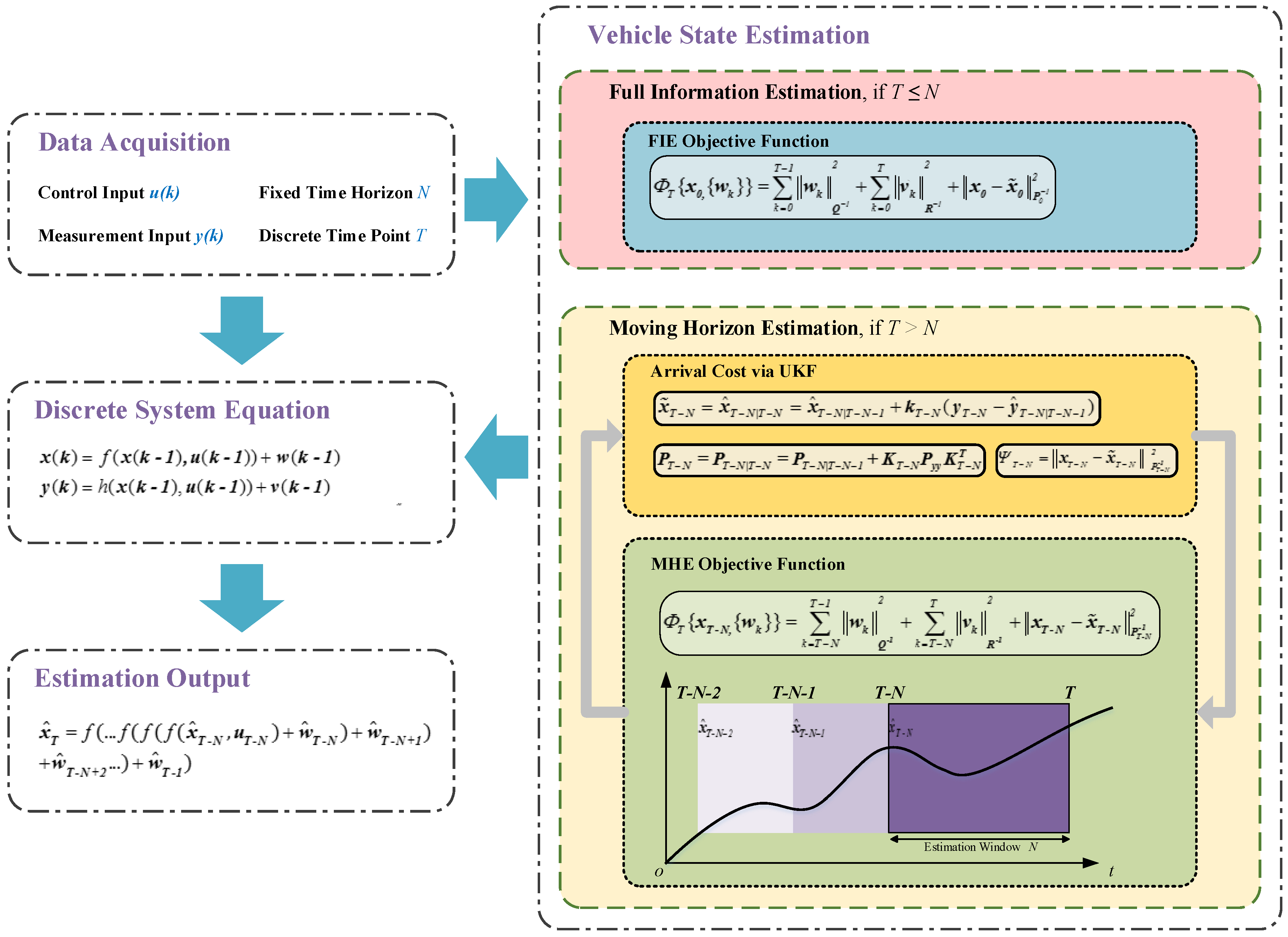
From the Bayesian theory point of view, the constrained state estimation problem can be formulated as the solution of a full information estimation (FIE) problem [35]. Therefore, the FIE objective function for Equation (22) is written as:
subject to
where ; is the state disturbance sequence from time k = 0 to k = T − 1; and is the initial estimate of vehicle states with corresponding covariance matrix .
Additionally, it is worth noting that, in practice, the vehicle speed should be less than on driving conditions and greater than on braking conditions. However, measurement noise or some other reasons may occasionally result in accidental error, which affects the accuracy of the subsequent estimation. Thus, the following additional constraints for the vehicle longitudinal velocity are given and applied to reduce this effect:
However, real-time implementations of FIE are computationally infeasible due to the infinite growth of the number of sampling points. To make the objective function tractable, the estimation size needs to be bounded. One common strategy to estimate the instead of the full-state sequence , where N is the fixed time horizon of Equation (39), just like a moving “sampling window”. Therefore, Equation (39) is rewritten as,
where is the arrival cost that incorporates estimate information prior to the horizon, namely from time k = 0 to time k = T − N − 1. Therefore, the arrival cost is indeed necessary for the application of MHE. For nonlinear systems like Equation (22), however, general analytical expressions of the arrival cost are unavailable. Methods for formulating the arrival cost include EKF, UKF, or even discarding the arrival cost by taking it as a constant value. In this study, an UKF-based arrival cost calculation approach [36] is applied. Differently from the UKF described in Section 3.1, for the constrained problem, the selection of sigma points takes the parameter constraints into account so that none of the selected sigma points violate the boundaries of the state variables:
where , and . ri is the step size in each direction of the set of sigma points with constraints, which is calculated as follows [36]:
where , are the upper and lower bounds in the direction.
As the sigma points are obtained, and can be updated via the UKF equation described in Section 3.1.
The arrival cost can be calculated as follows:
Finally, the whole process of MHE-based state estimation algorithm is shown in Figure 3 and explained in the form of pseudocode in Algorithm 1.
| Algorithm 1. Pseudocode of moving horizon estimation algorithm | |
| 1. | Initialization: set the initial values for and the horizon length N. |
| 2. | Prepare for estimation: increment and obtain the current measurement input and control input . |
| 3. | Estimation: if |
| Solve Equation (39) as full information estimation; | |
| else | |
| Compute the UKF gain matrix and update via UKF; | |
| Compute the arrival cost ; | |
| Solve Equation (41) with the obtained arrival cost . | |
| end | |
| 4. | Results output: compute states in the horizon, |
| 5. | End of estimation: go to Step 2. |
4. Simulation Results and Analysis
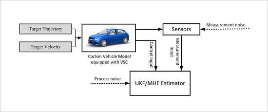
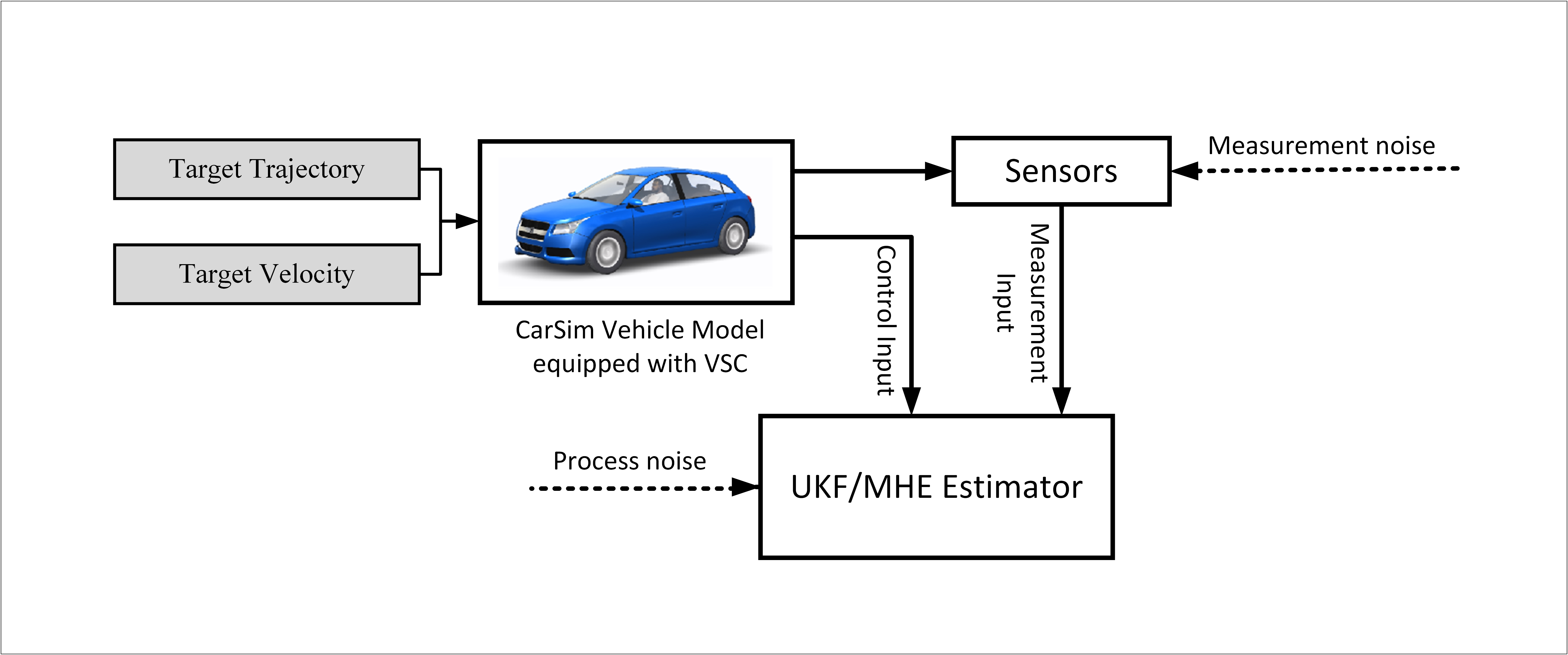
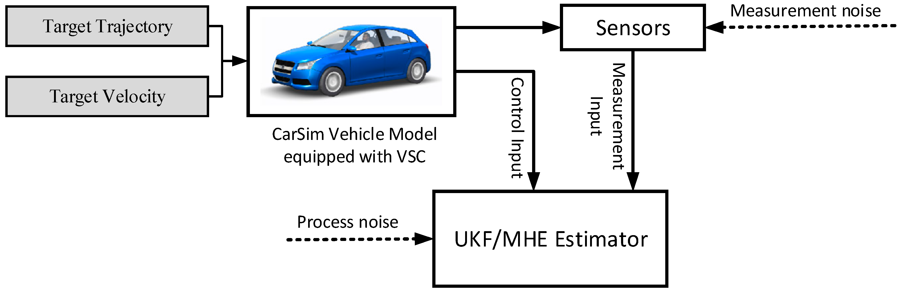
In order to evaluate and compare the presented estimation algorithms, computer simulations are implemented in the environment of CarSim combined with Matlab/Simulink, as shown in Figure 4. CarSim is commercial vehicle dynamic software. The vehicle model in CarSim contains a steering system, tires, and driver model, and is extensively validated and correlated to real-world results, as measured and observed by many automotive OEMs around the world. Therefore, in this study, the embedded vehicle model equipped with VSC in CarSim serves as a real vehicle, providing control input, reference vehicle states and measured signals, while the estimation algorithms are built in Matlab/Simulink. The vehicle parameters used in the simulation are listed in Table 1. 5% differences of these parameters are added to the UKF 3-DOFs vehicle model in the simulation to imitate modeling uncertainties.
4.1. Initial Settings of Simulations
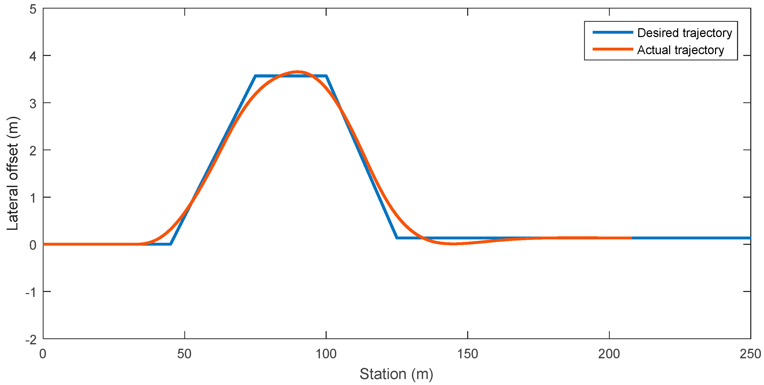
In this section, an emergency double lane change (DLC) test (ISO3888-1:1999) is simulated with a driver preview time of 0.5 s, which is a short but appropriate value for an emergency situation. The desired longitudinal velocity is 100 km/h controlled and the tire/road friction coefficient is set as 0.8. Such a critical driving condition should be persuasive, since the lateral vehicle motion response has a relatively large variation scale. VSC guarantees that the vehicle passes the DLC test successfully.
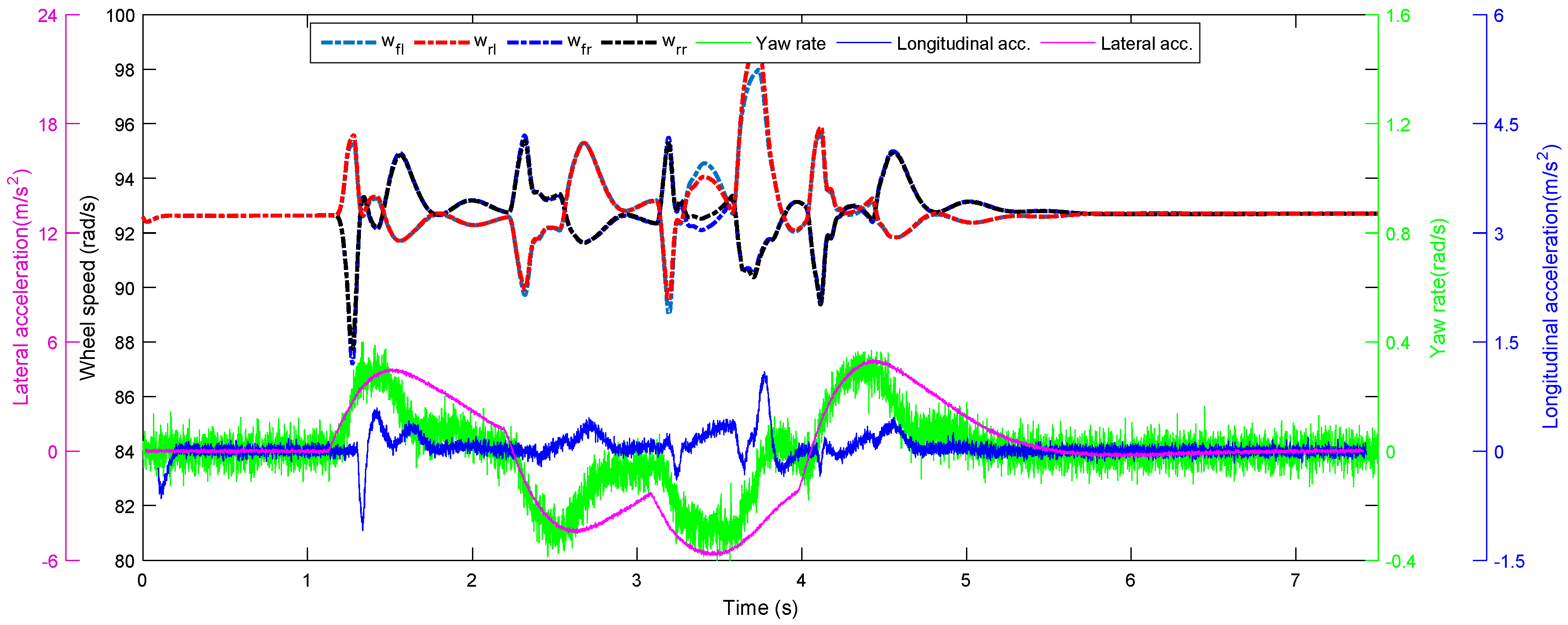
In the simulation process, the sensor signals are assumed to be obtained in real time. Furthermore, Gaussian noise is added to the simulated measurements to realistically represent the real application. The standard deviation of longitudinal acceleration sensor noise is 5 × 10⁻² m/s2; the standard deviation of lateral acceleration sensor noise is 5 × 10⁻² m/s2; the standard deviation of yaw rate sensor noise is 2.4°/s; the standard deviation of wheel rotational velocity noise is 10−3 rad/s [37].
In addition, the parameters used in the UKF and MEH design are very important for the performance of the proposed estimators. Some design principles have been well investigated [28,38,39]. According to the recommended options and our own tests, the parameters are given as follows: , , and the fixed time horizon . Furthermore, the parameters used in the UKF-based arrival cost calculation in MHE are the same as the UKF estimator’s parameters.
4.2. Results Analysis
Figure 5 shows the tracking performance of the targeted driving process. The CarSim vehicle model equipped with VSC is able to accomplish the designed double lane change maneuver with acceptable tracking accuracy.
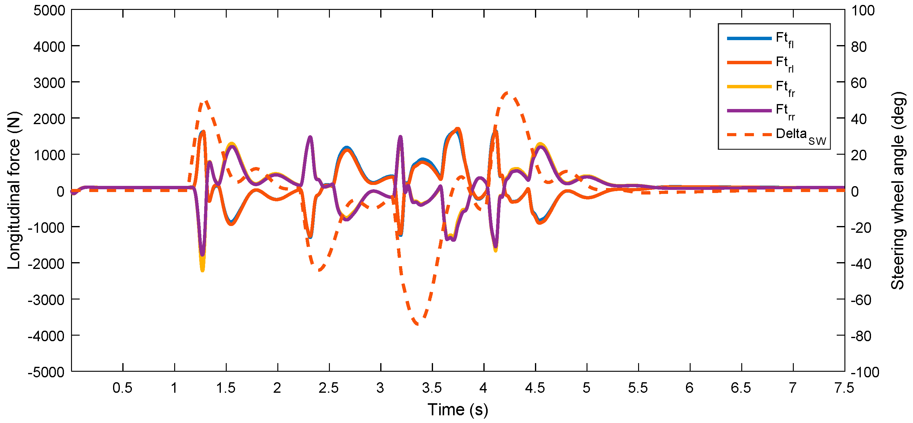
Using the torque and rotational speed information directly acquired from CarSim, the longitudinal force of each tire can be calculated according to Equation (2). These longitudinal forces combined with the hand wheel steering angle signal comprise the control input, shown in Figure 6. Additionally, the measurements from virtual sensors under DLC test are depicted in Figure 7.
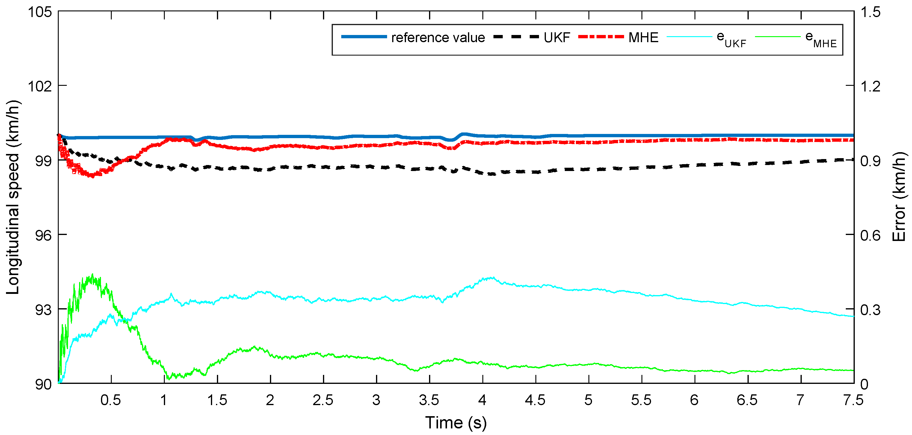
UKF and MHE are implemented as two separate methods in order to directly compare the estimation performance and robustness. Figure 8, Figure 9, Figure 10 and Figure 11 show the estimated results and errors of the longitudinal velocity, lateral velocity, yaw rate, and lateral tire forces, respectively, using these two estimation methods,. Figure 8 shows that both MHE and UKF can estimate the longitudinal speed satisfactorily. However, MHE shows a faster convergence and slightly higher accuracy compared with UKF.
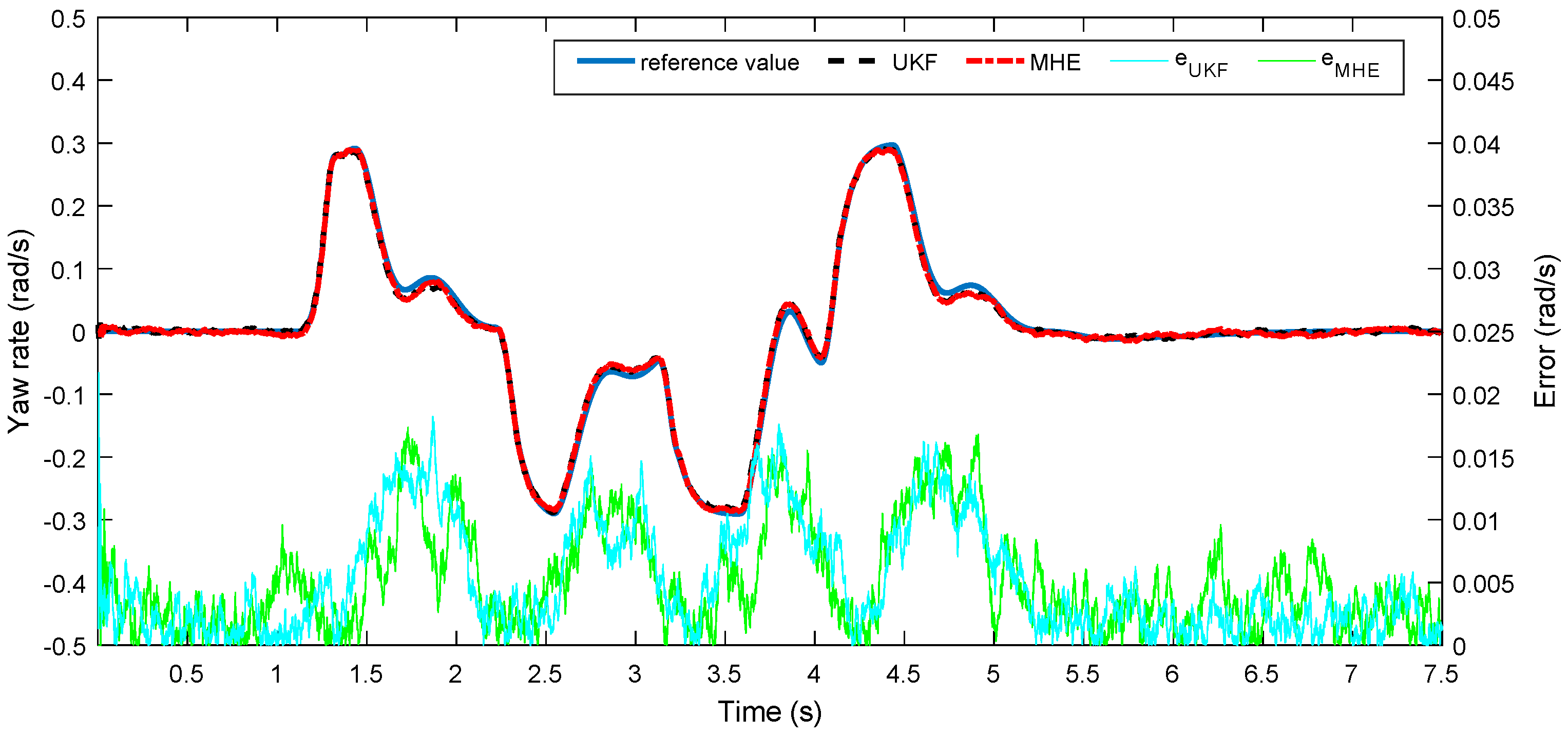
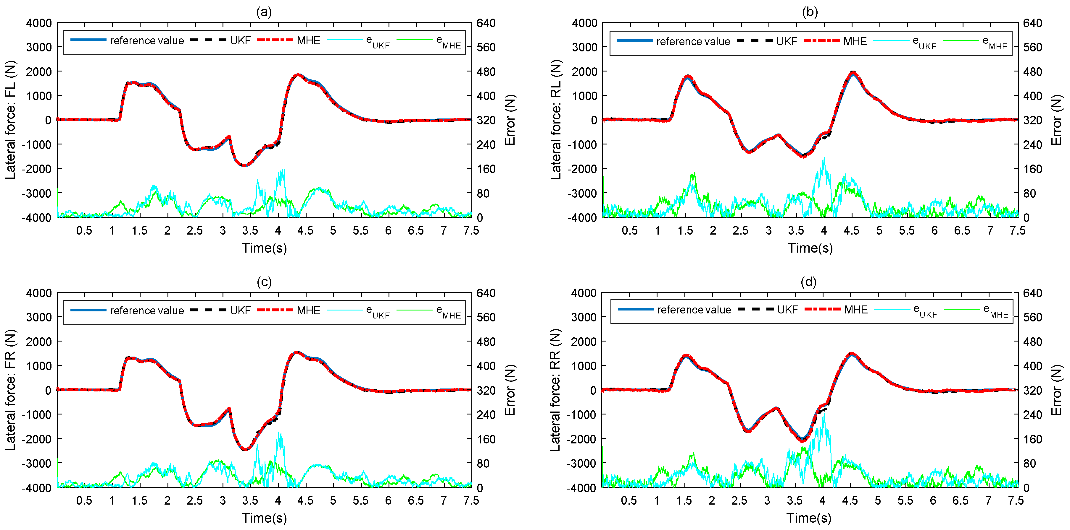
During the lane changing interval around 4 s where the hand wheel input and lateral acceleration vary greatly, it can be seen from Figure 9 that UKF and MHE perform differently; near 4 s the estimated error of UKF is relatively larger and more fluctuating than that of MHE. Regarding the yaw rate estimation, the overall performance of both algorithms is satisfactory, as seen in Figure 10. Similar to the situation of lateral speed estimation, for the lateral tire force estimation in Figure 11, MHE also shows better performance than UKF under the strong nonlinearity caused by the large lateral acceleration.
Table 2 summarizes the quantitative analysis for both UKF and MHE algorithms, including ME (maximum estimation) error, RMS (root mean square) error, and improvement percentage. Except that the longitudinal speed ME error of MHE is a bit larger than that of UKF, MHE outperforms UKF in all other cases. The ME errors of estimated states drop significantly when MHE is applied. Meanwhile, compared with UKF, the RMS errors of these seven vehicle states are improved at least 10% by MHE. For the longitudinal speed, the improvement even reaches 62%.
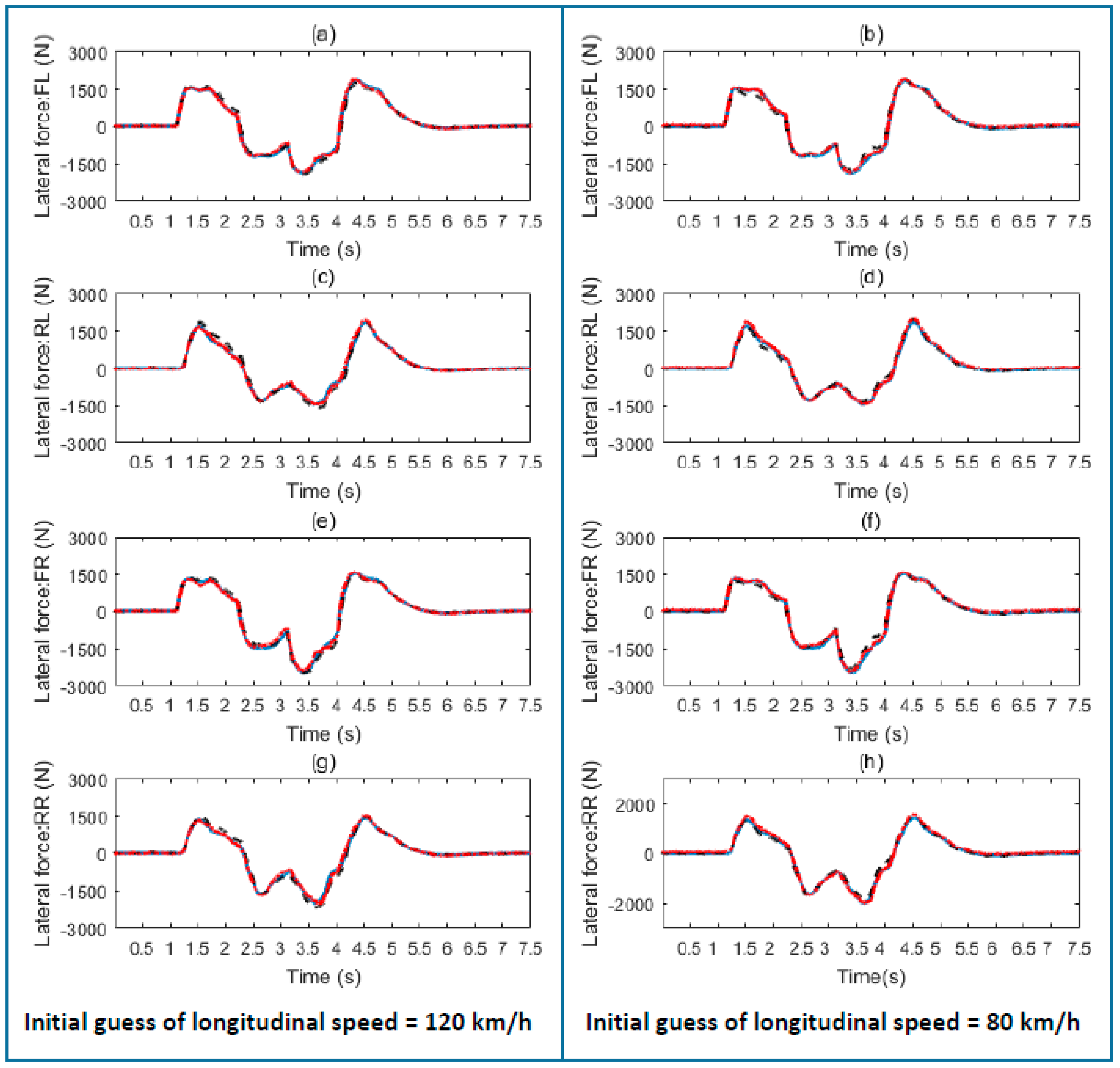
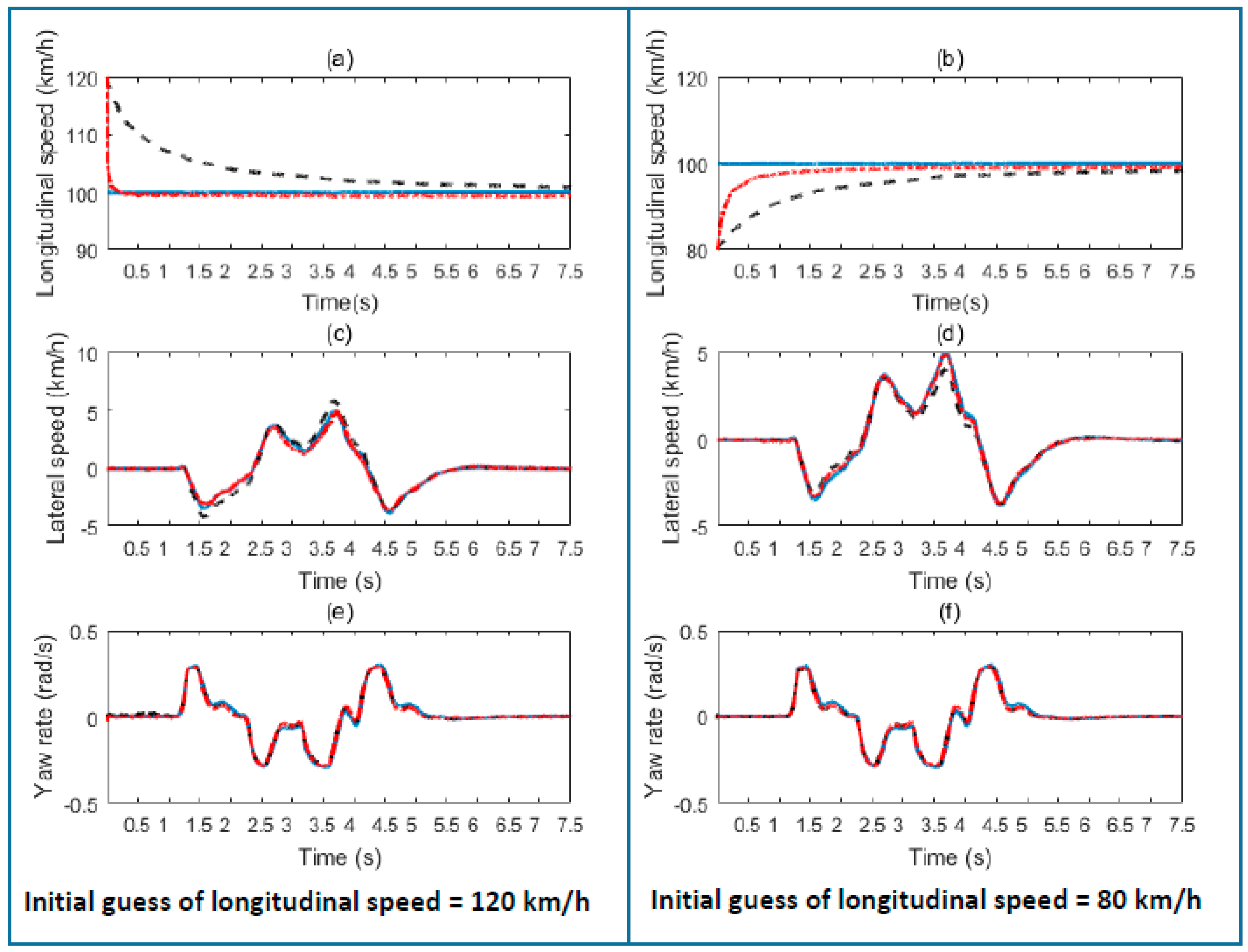
It is noteworthy that in real applications, measurement noise or other reasons may occasionally result in a wrong initial state value, which affects the accuracy of the subsequent estimation. In order to further evaluate the robustness of these two estimation algorithms, simulations with incorrect initial longitudinal speed estimates of 120 km/h and 80 km/h are conducted, the results of which are illustrated in Figure 12 and Figure 13. Compared to UKF, MHE has the advantage of solving this kind of constrained state estimation problem. In this study, the constraint is set as Equation (40) in Section 3.2.
In Figure 12a,c,e are the estimation with the initial value of 120 km/h and Figure 12b,d,f with the initial value of 80 km/h. Due to Equation (40), the estimated longitudinal speed by MHE approach converges to the reference value rapidly when the initial estimate equals 120 km/h. Even under an initial estimate of 80 km/h, MHE still converges faster than UKF. The other vehicle states, such as lateral speed, yaw rate, and lateral tire forces in Figure 13, are not affected too much by the wrong initial longitudinal velocity estimate.
In Table 3 the ME error and RMS error of each state variable are listed. Combining Table 2 with the calculated results, we find that, for both the MHE and UKF algorithms, the estimation with wrong initial longitudinal velocity performs slightly worse than that with a correct initial estimate. Even so, MHE still shows more robustness and a faster convergence ability than UKF.
5. Conclusions and Future Work
This study presented and compared two algorithms, UKF and MHE, for the vehicle longitudinal velocity, lateral velocity, yaw rate, and tire lateral force estimating of DDEVs. Even though today some of these vehicle states can be directly measured by optical sensors or GPS sensors, some practical issues such as cost, accuracy, and reliability inhibit production vehicles from using these sensors at present or in the near future. In contrast, our proposed estimation algorithms are designed based on the information fusion combining feedback signals of electric motors and the existing standard sensor unit equipped in today’s typical vehicles. In some vehicle stability controller studies such as [40,41,42,43], it can replace expensive optical or GPS sensors as a cost-efficient way of providing accurate vehicle state information including velocities, yaw rate, sideslip angle, and tire lateral forces.
In this article, the mathematical vehicle model was established based on 3-DOFs planar vehicle model with a simplified “Pacejka 2002” tire model. Computer simulations are conducted under the emergency DLC test in the co-environment of CarSim and Simulink to evaluate the performance of designed estimators. It is supposed to be persuasive, since during this maneuver vehicle states show large variation. Based on the analysis of the simulation results, our findings are summarized as follows.
- (1)
- The estimation results for vehicle states including the longitudinal velocity, lateral velocity, yaw rate, and lateral tire forces, by both UKF and MHE, are satisfactory.
- (2)
- Compared with UKF, MHE has better estimation accuracy, especially under serious nonlinear situations.
- (3)
- MHE has faster convergence ability and is more robust against an incorrect initial estimate of the longitudinal velocity.
As a future research topic, estimation on rolling movement will be taken into consideration, which is of great significance for the rollover prevention control. Furthermore, our prototype vehicle is currently in the design and manufacturing stage. Field tests need to be carried out in the future to verify the proposed estimation algorithms.
Acknowledgments
The work as supported by the BCV project (Berlin City Vehicle Project) of the Technical University of Berlin. The authors would like to thank the China Scholarship Council (CSC) for providing the financial support (201306030007) for Xudong Zhang to pursue his Ph.D. degree at TU Berlin. We acknowledge support by the German Research Foundation and the Open Access Publication Funds of Technische Universität Berlin.
Author Contributions
Xudong Zhang and Dietmar Göhlich proposed the conception and design of this study. Dietmar Göhlich provided the resources and software. Xudong Zhang built the vehicle model and tire model and designed the unscented Kalman filter. Chenrui Fu designed the moving horizon estimator. Xudong Zhang and Chenrui Fu carried out the simulations. All authors conducted the data analysis, discussed the results, and contributed to writing and reviewing the manuscript.
Conflicts of Interest
The authors declare that there is no conflict of any competing financial interests regarding the publication of this paper.
Nomenclature
| a | Distance from center of gravity (COG) to front wheels |
| Longitudinal acceleration | |
| Lateral acceleration | |
| A | Frontal projected area |
| b | Distance from COG to rear wheels |
| Air resistance coefficient | |
| Lateral tire force | |
| Longitudinal tire force | |
| Resultant tire force alone x-axis | |
| Resultant tire force alone y-axis | |
| Tire normal load | |
| h | Height of sprung mass center of gravity |
| i | Transmission ratio from motor to wheel |
| is | Transmission ratio from the hand wheel to front wheels |
| Iz | Vehicle rotational inertia about z-axis |
| Wheel rotational inertia | |
| l | Wheelbase |
| m | Gross mass |
| r | Yaw rate |
| R | Wheel radius |
| T | Wheel track |
| Motor torque output | |
| Longitudinal vehicle velocity | |
| Wheel center speed | |
| Lateral vehicle velocity | |
| Wheel rotational speed | |
| Motor rotational speed | |
| Tire side slip angle | |
| Tire slip ratio | |
| Air density | |
| Steering wheel angle | |
| Steering angle of each wheel | |
| ij = fl,rl,fr,rr | The wheel position: front left, rear left, front right, and rear right |
References
- Chu, W.; Luo, Y.; Dai, Y.; Li, K. In–wheel motor electric vehicle state estimation by using unscented particle filter. Int. J. Veh. Des. 2015, 67, 115–136. [Google Scholar] [CrossRef]
- Bahouth, G. Real World Crash Evaluation of Vehicle Stability Control (VSC) Technology. Annu. Proc. Assoc. Adv. Automot. Med. 2005, 49, 19–34. [Google Scholar] [PubMed]
- Van Zanten, A.T. Evolution of electronic control systems for improving the vehicle dynamic behavior. In Proceedings of the 6th International Symposium on Advanced Vehicle Control, Hiroshima, Japan, 9–13 September 2002; pp. 1–9. [Google Scholar]
- Sun, C.; Hu, X.; Moura, S.J.; Sun, F. Velocity Predictors for Predictive Energy Management in Hybrid Electric Vehicles. IEEE Trans. Control Syst. Technol. 2015, 23, 1197–1204. [Google Scholar]
- Zhang, X.; Göhlich, D. Integrated Traction Control Strategy for Distributed Drive Electric Vehicles with Improvement of Economy and Longitudinal Driving Stability. Energies 2017, 10, 126. [Google Scholar] [CrossRef]
- Venhovens, P.J.T.; Naab, K. Vehicle Dynamics Estimation Using Kalman Filters. Veh. Syst. Dyn. 1999, 32, 171–184. [Google Scholar] [CrossRef]
- Daiss, A.; Kiencke, U. Estimation of vehicle speed fuzzy-estimation in comparison with Kalman-filtering. In Proceedings of the 4th IEEE Conference on Control Applications, Albany, NY, USA, 28–29 September 1995; pp. 281–284. [Google Scholar]
- Du, X.P.; Lu, L.T.; Sun, H.M.; Li, Y.; Song, J.J. A Vehicle Rollover Warning Approach Based on Neural Network and Support Vector Machine. Appl. Mech. Mater. 2013, 367, 433–440. [Google Scholar] [CrossRef]
- Sasaki, H.; Nishimaki, T. A Side-Slip Angle Estimation Using Neural Network for a Wheeled Vehicle. SAE trans. 2000, 109, 1026–1031. [Google Scholar] [CrossRef]
- Wei, W.; Shaoyi, B.; Lanchun, Z.; Kai, Z.; Yongzhi, W.; Weixing, H. Vehicle Sideslip Angle Estimation Based on General Regression Neural Network. Math. Probl. Eng. 2016, 2016. [Google Scholar] [CrossRef]
- Liu, W.; He, H.; Sun, F. Vehicle state estimation based on Minimum Model Error criterion combining with Extended Kalman Filter. J. Frankl. Inst. 2016, 353, 834–856. [Google Scholar] [CrossRef]
- Hac, A.; Simpson, M.D. Estimation of vehicle side slip angle and yaw rate. SAE Trans. 2000, 109, 1032–1038. [Google Scholar] [CrossRef]
- Farrelly, J.; Wellstead, P. Estimation of vehicle lateral velocity. In Proceedings of the 1996 IEEE International Conference on Control Applications, Dearborn, MI, USA, 15 September–18 November 1996; pp. 552–557. [Google Scholar]
- Guo, H.; Ma, B.; Ma, Y.; Chen, H. Modular scheme for vehicle tire forces and velocities estimation based on sliding mode observer. In Proceedings of the 2016 Chinese Control and Decision Conference (CCDC), Yinchuan, China, 28–30 May 2016; pp. 5661–5666. [Google Scholar]
- Chen, Y.; Ji, Y.; Guo, K. A reduced-order nonlinear sliding mode observer for vehicle slip angle and tyre forces. Veh. Syst. Dyn. 2014, 52, 1716–1728. [Google Scholar] [CrossRef]
- Veluvolu, K.C.; Rath, J.J.; Defoort, M.; Soh, Y.C. Estimation of side slip and road bank angle using high-gain observer and higher-order sliding mode observer. In Proceedings of the 2015 International Workshop on Recent Advances in Sliding Modes (RASM), Istanbul, Turkey, 9–11 April 2015; pp. 1–6. [Google Scholar]
- Sun, J.; Ding, S.; Zhang, S.; Zheng, W.X. Nonsmooth stabilization for distributed electric vehicle based on direct yaw-moment control. In Proceedings of the 2016 35th Chinese Control Conference (CCC), Chengdu, China, 27–29 July 2016; pp. 8850–8855. [Google Scholar]
- Xiong, L.; Yu, Z.; Wang, Y.; Yang, C.; Meng, Y. Vehicle dynamics control of four in-wheel motor drive electric vehicle using gain scheduling based on tyre cornering stiffness estimation. Veh. Syst. Dyn. 2012, 50, 831–846. [Google Scholar] [CrossRef]
- Kalman, R.E.; Bucy, R.S. New Results in Linear Filtering and Prediction Theory. J. Basic Eng. 1961, 83, 95–108. [Google Scholar] [CrossRef]
- Pengov, M.; d’Andréa-Novel, B.; Fenaux, E.; Grazi, S.; Zarka, F. A comparison study of two kinds of observers for a vehicle. In Proceedings of the 2001 European Control Conference (ECC), Porto, Portugal, 4–7 September 2001; pp. 1068–1073. [Google Scholar]
- Wenzel, T.A.; Burnham, K.J.; Blundell, M.V.; Williams, A.R. Dual extended Kalman filter for vehicle state and parameter estimation. Veh. Syst. Dyn. 2006, 44, 153–171. [Google Scholar] [CrossRef]
- Chen, B.C.; Hsieh, F.C. Sideslip angle estimation using extended Kalman filter. Veh. Syst. Dyn. 2008, 46, 353–364. [Google Scholar] [CrossRef]
- Hamann, H.; Hedrick, J.K.; Rhode, S.; Gauterin, F. Tire force estimation for a passenger vehicle with the unscented kalman filter. In Proceedings of the 2014 IEEE Intelligent Vehicles Symposium, Dearborn, MI, USA, 8–11 June 2014; pp. 814–819. [Google Scholar]
- Ren, H.; Chen, S.; Liu, G.; Zheng, K. Vehicle State Information Estimation with the Unscented Kalman Filter. Adv. Mech. Eng. 2015, 6, 589397. [Google Scholar] [CrossRef]
- Antonov, S.; Fehn, A.; Kugi, A. Unscented Kalman filter for vehicle state estimation. Veh. Syst. Dyn. 2011, 49, 1497–1520. [Google Scholar] [CrossRef]
- Doumiati, M.; Victorino, A.C.; Charara, A.; Lechner, D. Onboard Real-Time Estimation of Vehicle Lateral Tire #x2013; Road Forces and Sideslip Angle. IEEE/ASME Trans. Mech. 2011, 16, 601–614. [Google Scholar]
- Julier, S.J.; Uhlmann, J.K. New extension of the Kalman filter to nonlinear systems. In Proceedings of the AeroSense 97 Conference on Photonic Quantum Computing, Orlando, FL, USA, 20–25 April 1997; pp. 182–193. [Google Scholar]
- Wan, E.A.; Van Der Merwe, R. The unscented Kalman filter for nonlinear estimation. In Proceedings of the IEEE 2000 Adaptive Systems for Signal Processing, Communications, and Control Symposium (AS-SPCC), Lake Louise, AB, Canada, 4 October 2000; pp. 153–158. [Google Scholar]
- Rawlings, J.B.; Bakshi, B.R. Particle filtering and moving horizon estimation. Comput. Chem. Eng. 2006, 30, 1529–1541. [Google Scholar] [CrossRef]
- Zanon, M.; Frasch, J.V.; Diehl, M. Nonlinear moving horizon estimation for combined state and friction coefficient estimation in autonomous driving. In Proceedings of the 2013 European Control Conference (ECC), Zurich, Switzerland, 17–19 July 2013; pp. 4130–4135. [Google Scholar]
- Kraus, T.; Ferreau, H.J.; Kayacan, E.; Ramon, H.; De Baerdemaeker, J.; Diehl, M.; Saeys, W. Moving horizon estimation and nonlinear model predictive control for autonomous agricultural vehicles. Comput. Electron. Agric. 2013, 98, 25–33. [Google Scholar] [CrossRef]
- Pacejka, H.B. Tyre and Vehicle Dynamics; Butterworth-Heinemann: Oxford, UK, 2006. [Google Scholar]
- Zhang, X.; Göhlich, D. A hierarchical estimator development for estimation of tire-road friction coefficient. PLoS ONE 2017, 12, e0171085. [Google Scholar] [CrossRef] [PubMed]
- Spivey, B.J.; Hedengren, J.D.; Edgar, T.F. Constrained Nonlinear Estimation for Industrial Process Fouling. Ind. Eng Chem. Res. 2010, 49, 7824–7831. [Google Scholar] [CrossRef]
- Rao, C.V.; Rawlings, J.B.; Mayne, D.Q. Constrained state estimation for nonlinear discrete-time systems: Stability and moving horizon approximations. IEEE Trans. Autom. Control 2003, 48, 246–258. [Google Scholar] [CrossRef]
- Qu, C.C.; Hahn, J. Computation of arrival cost for moving horizon estimation via unscented Kalman filtering. J. Process Control 2009, 19, 358–363. [Google Scholar] [CrossRef]
- Chu, W. State Estimation and Coordinated Control System. In State Estimation and Coordinated Control for Distributed Electric Vehicles; Springer: Berlin/Heidelberg, Germany, 2016; pp. 37–44. [Google Scholar]
- Julier, S.J.; Uhlmann, J.K.; Durrant-Whyte, H.F. A new approach for filtering nonlinear systems. In Proceedings of the 1995 American Control Conference, Seattle, WA, USA, 21–23 June 1995; Volume 3, pp. 1628–1632. [Google Scholar]
- Julier, S.J. The scaled unscented transformation. In Proceedings of the 2002 American Control Conference, Anchorage, AK, USA, 8–10 May 2002; Volume 6, pp. 4555–4559. [Google Scholar]
- Jiang, D.; Danhua, L.; Wang, S.; Tian, L.; Yang, L. Additional Yaw Moment Control of a 4WIS and 4WID Agricultural Data Acquisition Vehicle. Int. J. Adv. Robot. Syst. 2015, 12, 78. [Google Scholar] [CrossRef]
- Nakano, H.; Okayama, K.; Kinugawa, J.; Kosuge, K. Control of an electric vehicle with a large sideslip angle using driving forces of four independently-driven wheels and steer angle of front wheels. In Proceedings of the 2014 IEEE/ASME International Conference on Advanced Intelligent Mechatronics, Besacon, France, 8–11 July 2014; pp. 1073–1078. [Google Scholar]
- Weiskircher, T.; Müller, S. Control performance of a road vehicle with four independent single-wheel electric motors and steer-by-wire system. Veh. Syst. Dyn. 2012, 50, 53–69. [Google Scholar] [CrossRef]
- Zhou, Y.; Liu, W.; Ogai, H. Control of Yaw Angle and Sideslip Angle Based on Kalman Filter Estimation for Autonomous EV from GPS. In Proceedings of the International MultiConference of Engineers and Computer Scientists, Hong Kong, China, 15–17 March 2017; Volume 1. [Google Scholar]
Figure 1.
Planar vehicle model and coordinate systems.
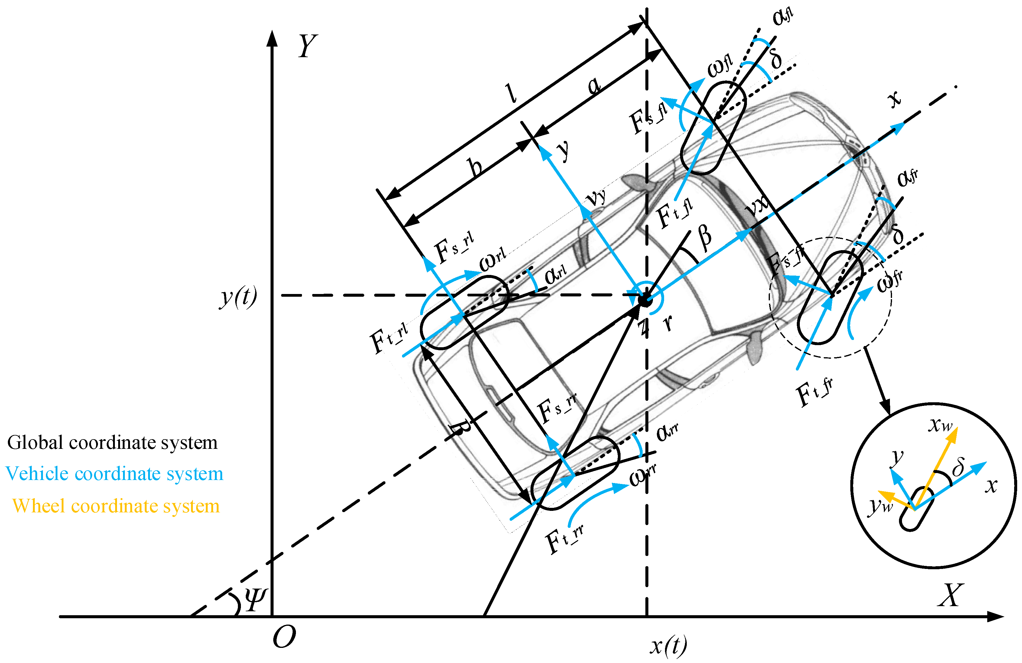
Figure 2.
The schematic of an unscented Kalman filter.
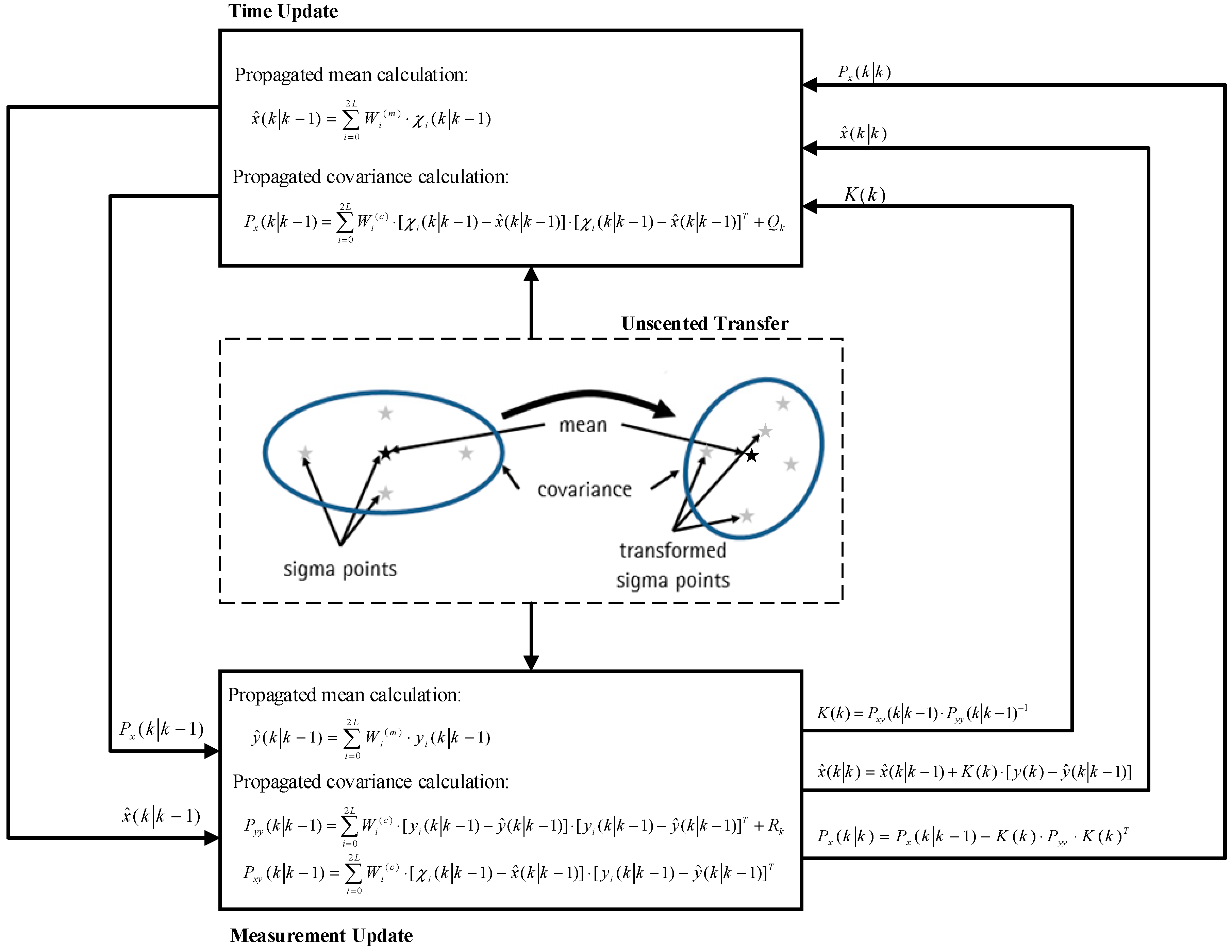
Figure 3.
Moving horizon estimation flowchart.

Figure 4.
Block diagram of the simulation system. UKF: unscented Kalman filter; MHE: moving horizon estimation.
Figure 4.
Block diagram of the simulation system. UKF: unscented Kalman filter; MHE: moving horizon estimation.

Figure 5.
Tracking results on the desired trajectory.

Figure 6.
Control input signals of the double lane change (DLC) maneuver.

Figure 7.
Measured signals with Gaussian noises.

Figure 8.
Estimated results and errors of longitudinal velocity using UKF and MHE.

Figure 9.
Estimated results and errors of lateral velocity using UKF and MHE.
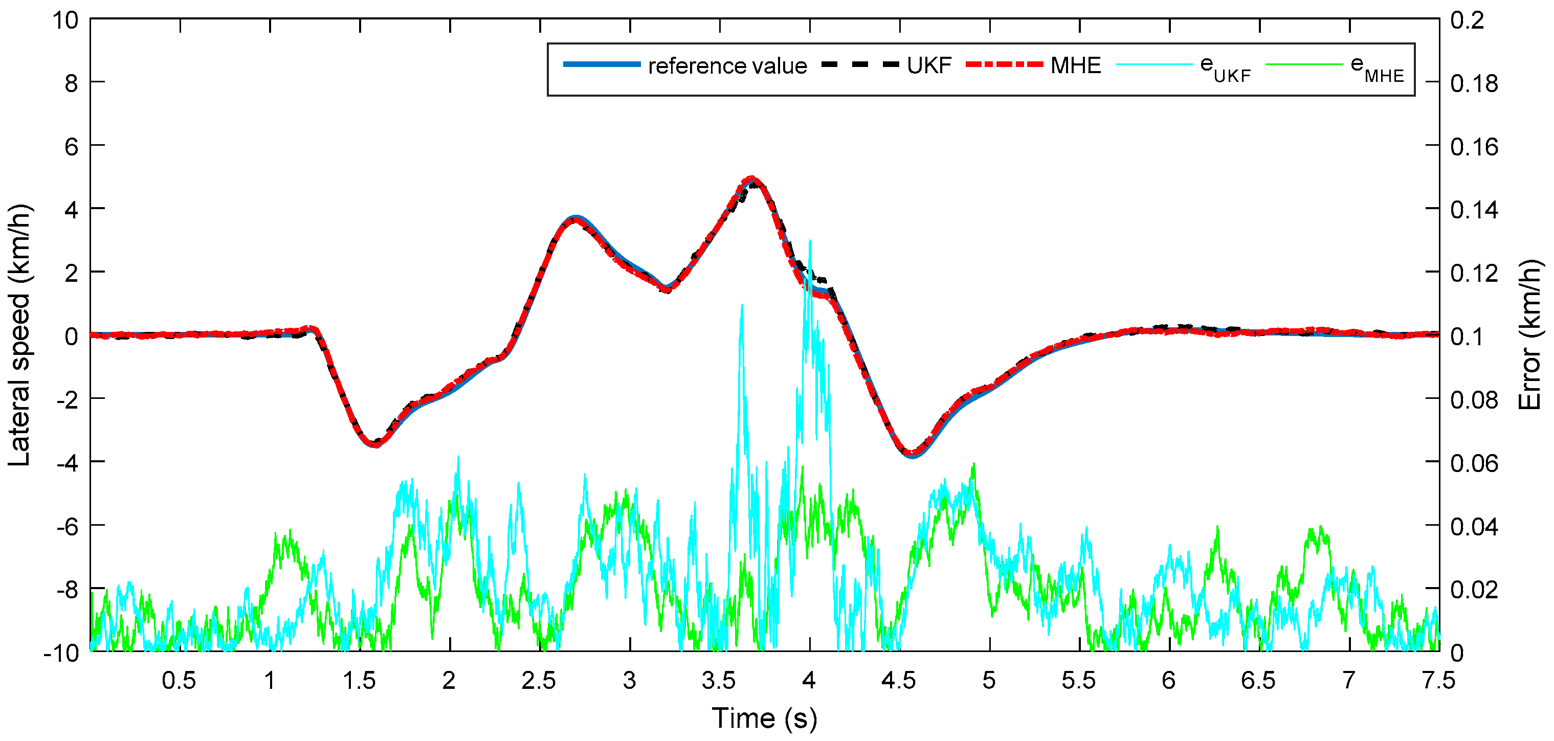
Figure 10.
Estimated results and errors of yaw rate using UKF and MHE.

Figure 11.
Estimated results and errors of tire lateral forces using UKF and MHE. (a) Estimated lateral tire force FL; (b) Estimated lateral tire force RL; (c) Estimated lateral tire force FR; (d) Estimated lateral tire force RR.
Figure 11.
Estimated results and errors of tire lateral forces using UKF and MHE. (a) Estimated lateral tire force FL; (b) Estimated lateral tire force RL; (c) Estimated lateral tire force FR; (d) Estimated lateral tire force RR.

Figure 12.
Estimation performance comparison using UKF and MHE with longitudinal velocity incorrectly initialized. (The red dashed line is estimated by MHE; the black dotted line is estimated by UKF; and the continuous blue line is the reference value). (a) Estimated longitudinal speed under initial guess of longitudinal speed 120 km/h; (b) Estimated longitudinal speed under initial guess of longitudinal speed 80 km/h; (c) Estimated lateral speed under initial guess of longitudinal speed 120 km/h; (d) Estimated lateral speed under initial guess of longitudinal speed 80 km/h; (e) Estimated yaw rate under initial guess of longitudinal speed 120 km/h; (f) Estimated yaw rate under initial guess of longitudinal speed 80 km/h.

Figure 13.
Estimation performance comparison using UKF and MHE with longitudinal velocity incorrectly initialized. (The red dashed line is estimated by MHE; the black dotted line is estimated by UKF; and the continuous blue line is the reference value). (a) Estimated lateral tire force FL under initial guess of longitudinal speed 120 km/h; (b) Estimated lateral tire force FL under initial guess of longitudinal speed 80 km/h; (c) Estimated lateral tire force RL under initial guess of longitudinal speed 120 km/h; (d) Estimated lateral tire force RL under initial guess of longitudinal speed 80 km/h; (e) Estimated lateral tire force FR under initial guess of longitudinal speed 120 km/h; (f) Estimated lateral tire force FR under initial guess of longitudinal speed 80 km/h; (g) Estimated lateral tire force RR under initial guess of longitudinal speed 120 km/h; (h) Estimated lateral tire force RR under initial guess of longitudinal speed 80 km/h.

Table 1.
Vehicle parameters. COG: center of gravity.
| Parameter | Unit | Value |
|---|---|---|
| Gross Mass | m (kg) | 1280 |
| Height of sprung mass center of gravity | h (m) | 0.5 |
| Distance from COG to front wheels | a (m) | 1.203 |
| Distance from COG to rear wheels | b (m) | 1.217 |
| Wheelbase | l (m) | 2.420 |
| Wheel track | T (m) | 1.330 |
| Wheel Radius | R (m) | 0.298 |
| Vehicle rotational inertia about z-axis | Iz (kg·m2) | 2500 |
| Transmission ratio from motor to wheel | i (-) | 4.5 |
| Transmission ratio from the hand wheel to front wheels | is (-) | 20 |
| Wheel rotational inertia | Jw (kg·m2) | 2.5 |
Table 2.
ME and RMS errors comparison of UKF and MHE on the DLC maneuver. ME: maximum estimation; RMS: root mean square.
Table 2.
ME and RMS errors comparison of UKF and MHE on the DLC maneuver. ME: maximum estimation; RMS: root mean square.
| State | ME Error | RMS Error | ||||
|---|---|---|---|---|---|---|
| MHE | UKF | Improvement | MHE | UKF | Improvement | |
| 0.441 | 0.428 | −3.037% | 0.127 | 0.335 | 62.090% | |
| 0.067 | 0.130 | 48.462% | 0.024 | 0.029 | 17.241% | |
| 0.017 | 0.022 | 22.727% | 0.006 | 0.007 | 14.286% | |
| 98.429 | 156.903 | 37.268% | 38.278 | 43.850 | 12.707% | |
| 145.710 | 195.451 | 25.449% | 44.730 | 49.941 | 10.434% | |
| 93.551 | 181.288 | 48.396% | 37.152 | 43.084 | 13.768% | |
| 135.059 | 241.798 | 44.144% | 44.949 | 55.750 | 19.374% | |
Table 3.
ME and RMS errors comparison of UKF and MHE on the DLC maneuver with an incorrect initial estimate of longitudinal velocity.
Table 3.
ME and RMS errors comparison of UKF and MHE on the DLC maneuver with an incorrect initial estimate of longitudinal velocity.
| Initial Velocity | ||||||||
|---|---|---|---|---|---|---|---|---|
| State | ME Error | RMS Error | ME Error | RMS Error | ||||
| MHE | UKF | MHE | UKF | MHE | UKF | MHE | UKF | |
| 5.555 | 5.547 | 0.264 | 1.408 | 5.556 | 5.546 | 0.752 | 1.703 | |
| 0.205 | 0.279 | 0.050 | 0.101 | 0.084 | 0.287 | 0.032 | 0.090 | |
| 0.031 | 0.046 | 0.012 | 0.013 | 0.025 | 0.029 | 0.011 | 0.013 | |
| 219.867 | 240.493 | 49.126 | 88.098 | 147.926 | 292.768 | 47.576 | 106.835 | |
| 235.481 | 299.550 | 54.423 | 105.462 | 201.060 | 231.921 | 58.604 | 83.239 | |
| 263.167 | 275.681 | 63.004 | 89.418 | 214.612 | 356.536 | 50.953 | 111.919 | |
| 297.239 | 366.145 | 59.385 | 111.808 | 182.882 | 275.438 | 56.724 | 87.101 | |
© 2017 by the authors. Licensee MDPI, Basel, Switzerland. This article is an open access article distributed under the terms and conditions of the Creative Commons Attribution (CC BY) license (http://creativecommons.org/licenses/by/4.0/).
Share and Cite
MDPI and ACS Style
Zhang, X.; Göhlich, D.; Fu, C. Comparative Study of Two Dynamics-Model-Based Estimation Algorithms for Distributed Drive Electric Vehicles. Appl. Sci. 2017, 7, 898. https://doi.org/10.3390/app7090898
AMA Style
Zhang X, Göhlich D, Fu C. Comparative Study of Two Dynamics-Model-Based Estimation Algorithms for Distributed Drive Electric Vehicles. Applied Sciences. 2017; 7(9):898. https://doi.org/10.3390/app7090898
Chicago/Turabian StyleZhang, Xudong, Dietmar Göhlich, and Chenrui Fu. 2017. "Comparative Study of Two Dynamics-Model-Based Estimation Algorithms for Distributed Drive Electric Vehicles" Applied Sciences 7, no. 9: 898. https://doi.org/10.3390/app7090898
Note that from the first issue of 2016, this journal uses article numbers instead of page numbers. See further details here.