Article

A Two-Stage Approach to Note-Level Transcription of a Specific Piano

1
Key Laboratory of Speech Acoustics and Content Understanding, Institute of Acoustics, Chinese Academyof Sciences, Beijing 100190, China
2
University of Chinese Academy of Sciences, Beijing 100190, China
3
Xinjiang Laboratory of Minority Speech and Language Information Processing, Xinjiang Technical Institute of Physics and Chemistry, Chinese Academy of Sciences, Urumchi 830001, China
*
Author to whom correspondence should be addressed.
Appl. Sci. 2017, 7(9), 901; https://doi.org/10.3390/app7090901
Submission received: 22 July 2017 / Revised: 25 August 2017 / Accepted: 29 August 2017 / Published: 2 September 2017
(This article belongs to the Special Issue Sound and Music Computing)

Abstract

:
This paper presents a two-stage transcription framework for a specific piano, which combines deep learning and spectrogram factorization techniques. In the first stage, two convolutional neural networks (CNNs) are adopted to recognize the notes of the piano preliminarily, and note verification for the specific individual is conducted in the second stage. The note recognition stage is independent of piano individual, in which one CNN is used to detect onsets and another is used to estimate the probabilities of pitches at each detected onset. Hence, candidate pitches at candidate onsets are obtained in the first stage. During the note verification, templates for the specific piano are generated to model the attack of note per pitch. Then, the spectrogram of the segment around candidate onset is factorized using attack templates of candidate pitches. In this way, not only the pitches are picked up by note activations, but the onsets are revised. Experiments show that CNN outperforms other types of neural networks in both onset detection and pitch estimation, and the combination of two CNNs yields better performance than a single CNN in note recognition. We also observe that note verification further improves the performance of transcription. In the transcription of a specific piano, the proposed system achieves 82% on note-wise F-measure, which outperforms the state-of-the-art.

1. Introduction

Automatic music transcription (AMT) is a process of transcribing a musical audio signal into a symbolic representation, such as a piano roll or music score. It has many applications in music information retrieval, composition, music education, and music visualization.
AMT has been researched for four decades (since 1977) [1,2], and it is still a challenging problem. While the transcription of monophonic music is considered solved, polyphonic AMT remains open because the signal is more complex. In polyphonic music, many notes overlap in the time domain and interact in the frequency domain. Additionally, the complexity of polyphony increases with the number of sound sources. For example, the concurrent notes in orchestral music come from instruments of different timbral properties, and the corresponding AMT performance is poor.
Note is the basic unit of music, and the main problem of transcription is to extract the information of every note in the music [3]. For each note, a set of information includes: pitch, onset, offset, loudness, and timbre. Pitch is a major attribute of auditory sensation, which can be reliably related to the fundamental frequency (F0). Onset refers to the beginning time of a note, and offset refers to the ending time. Loudness is the characteristic related to the amplitude of a sound. Timbre is that perceptual attribute in which a listener can judge that two sounds having the same loudness and pitch are dissimilar. In general, we only focus on which notes are played and when they appear in the music. Therefore, the pitch and onset time are necessary in the results of AMT.
The approaches to polyphonic transcription can be divided into frame-based methods and note-based methods [4]. The frame-based approaches estimate pitches in each time frame and form frame-level results in a post-processing stage. The most straightforward solution is to analyze the time–frequency representation of audio and compute the fundamental frequencies [5]. Short-time Fourier transform (STFT) [6,7] and constant Q transform (CQT) [8] are two widely used time–frequency analysis methods. Zhou proposed resonator time–frequency image (RTFI), in which a first-order complex resonator filter bank is adopted to the analysis of music [9]. Dressler used multi-resolution STFT, and the pitch was estimated by detecting peaks in the weighted spectrum [10]. Spectrogram factorization techniques are also very popular in AMT, such as non-negative matrix factorization (NMF) [11]. Probabilistic latent component analysis (PLCA) is another factorization technique, which aims to fit a latent variable probabilistic model to normalised spectrograms [12,13]. Apart from the discriminative approaches, deep neural networks have been used to identify pitches recently. Nam superimposed a support vector machine (SVM) on top of a deep belief network (DBN) to learn feature representations [14]. Sigtia compared the performance of neural networks and proposed a recurrent neural network (RNN) language model for music transcription [15]. Kelz utilized both a ConvNet and an AUNet in transcription, and investigated the glass ceiling effect of deep neural networks [16].
The note-based transcription approaches directly estimate notes, including pitches and onsets. One solution is combining the estimation of pitches and onsets into a single framework [17,18]. Kameoka [19] used harmonic temporal structured clustering to estimate the attributes of notes simultaneously. In [20], Böck used an RNN with bidirectional long short-term memory (LSTM) units. Similarly, Sigtia utilized three kinds of neural networks to transfer the input audio to a list of notes, along with the corresponding pitches and onset times [21]. Another solution is employing a separate onset detection stage and an additional pitch estimation stage. The approaches in this category often estimate the pitches using the segments between two successive onsets, and an accurate onset detection benefits the transcription. Marolt proposed a connectionist approach which contains a neural network of onset detection [22]. Costantini detected the onsets and estimated the pitches at the note attack using SVM [23]. However, little deep-learning-based research has been done in this category, to our knowledge.
Modeling the instrument being transcribed and learning the corresponding timbral properties is an efficient way to improve the AMT performance. Instrument-specific transcription research restricts the employed instrument models to a specific type. Depending on the timbral properties of different instruments, different sets of constraints are adopted in instrument-specific AMT systems [24,25,26]. As a typical multi-pitch instrument, the piano has been widely studied in AMT because its polyphony is challenging. The task of piano transcription has existed in MIREX (Music Information Retrieval Evaluation eXchange) since 2007, and it is competitive every year [27]. Figure 1 gives MIREX’s annual best results for the note tracking of piano subset based on onset only over the past 10 years. The current state-of-the-art system won 82% on F-measure in MIREX 2016, which is employed as a baseline system to evaluate the performance of our proposed method [28].
Individual-specific transcription is a new direction of AMT, which can make use of more characteristics of the individual piano. Cogliati and Duan modeled the temporal evolution of piano notes, and the spectrogram was factorized using the templates [29]. In the same context-dependent setting, they also employed convolutional sparse coding to transcribe the music from a specific piano in the specific environment [30]. In the supervised NMF, templates were usually formed by the isolated notes of the specific piano to be transcribed. Ewert employed spectro-temporal patterns to model the temporal evolution in NMF [31]. Cheng proposed a method to model the attack and decay of notes, and all the templates were trained by a Disklavier piano [32]. In the same transcription task, Gao combined the convolutional NMF with a differential spectrogram [33].
In this paper, we focus on the note-based polyphonic transcription for a specific piano. Deep learning technique is adopted to recognize notes preliminarily, and then the candidate notes are verified for the specific piano. In the stage of note recognition, a convolutional neural network (CNN) is used to detect onsets, and another CNN is used to estimate the probabilities of pitches at each detected onset. During the note verification, the spectrogram is factorized using attack templates of notes. Compared to existing AMT approaches, the proposed method has the following advantages:
(1)
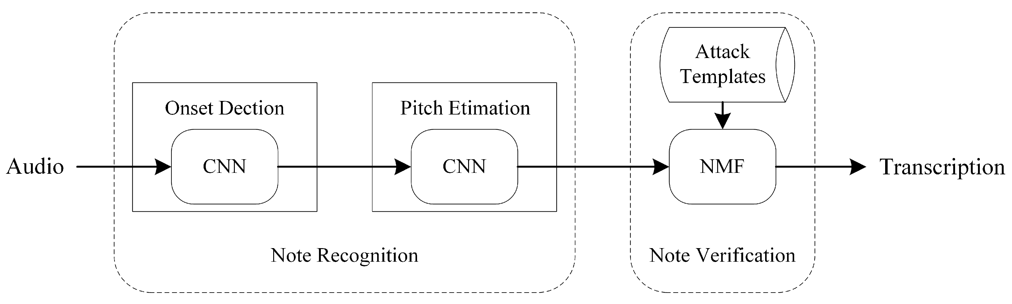
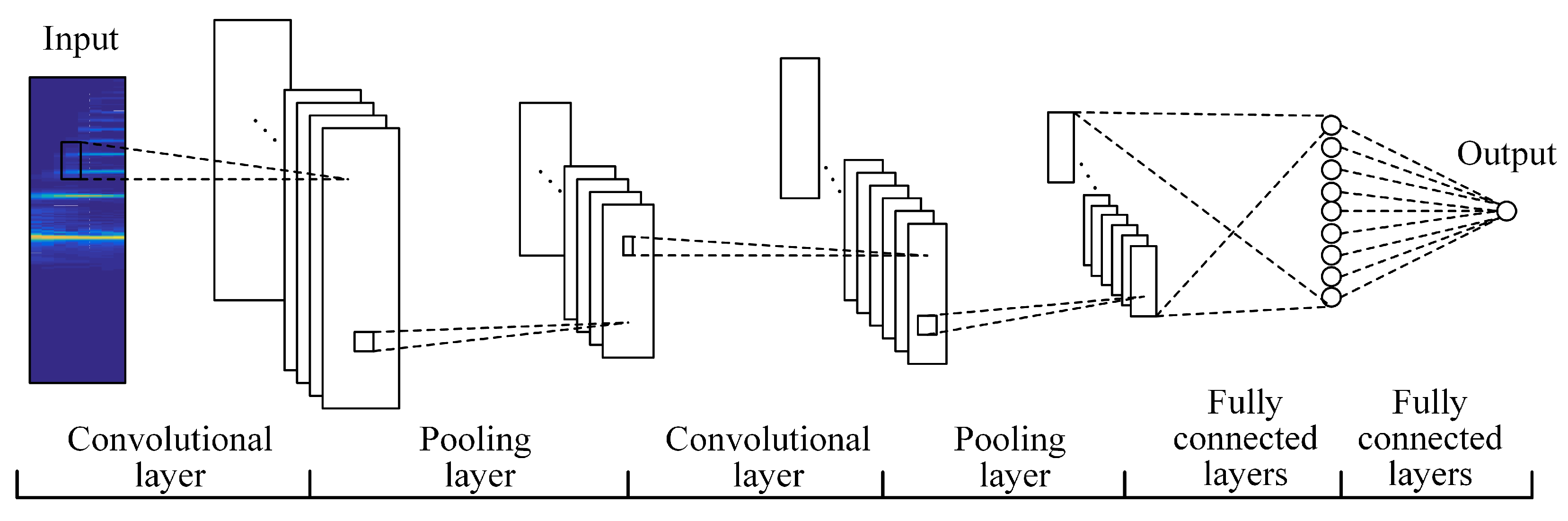
The note recognition stage yields a note-level transcription by estimating the pitch at each onset. Compared to existing deep-learning-based methods which use a single network, two consecutive CNNs yield better performance.
(2)
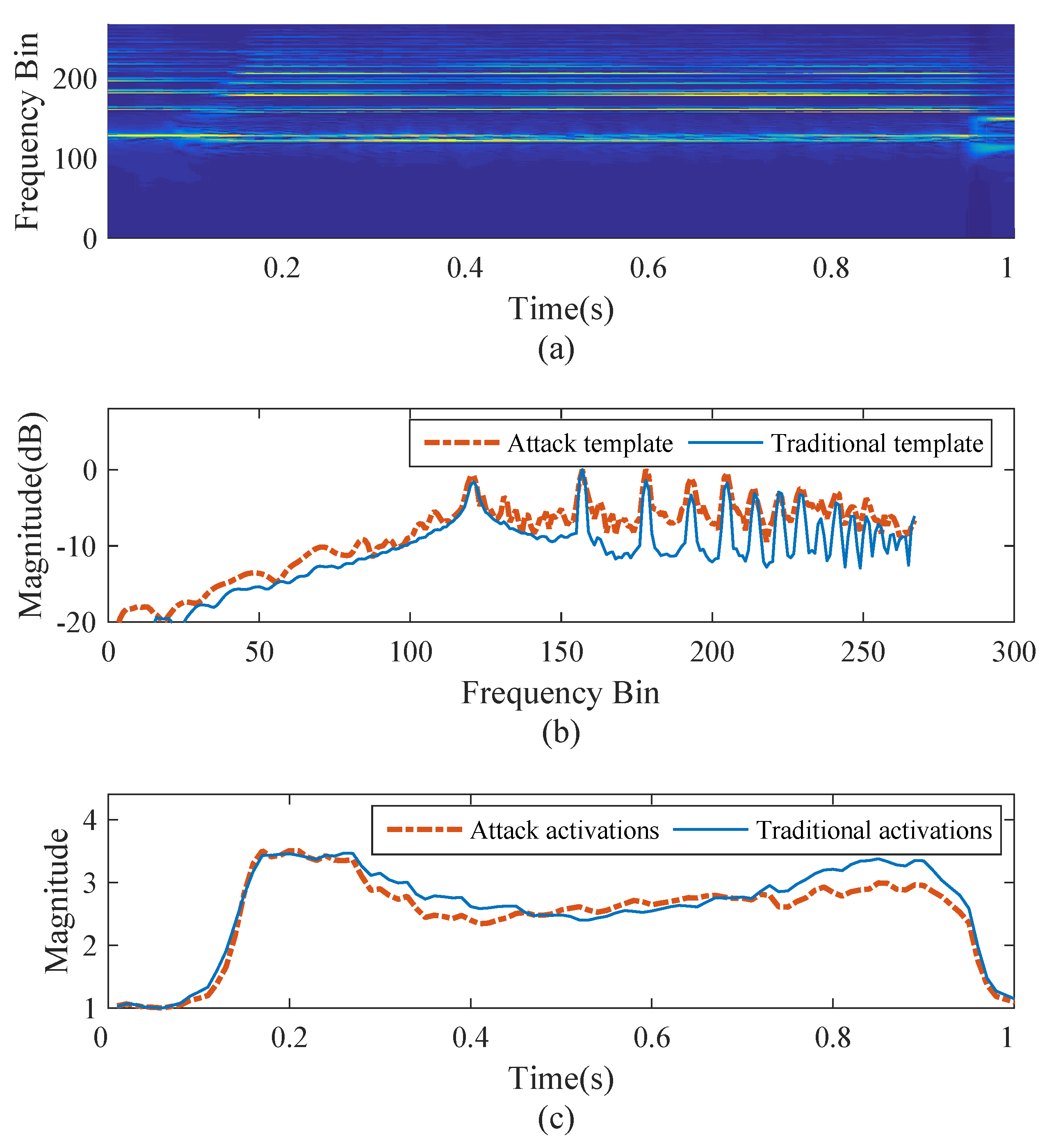
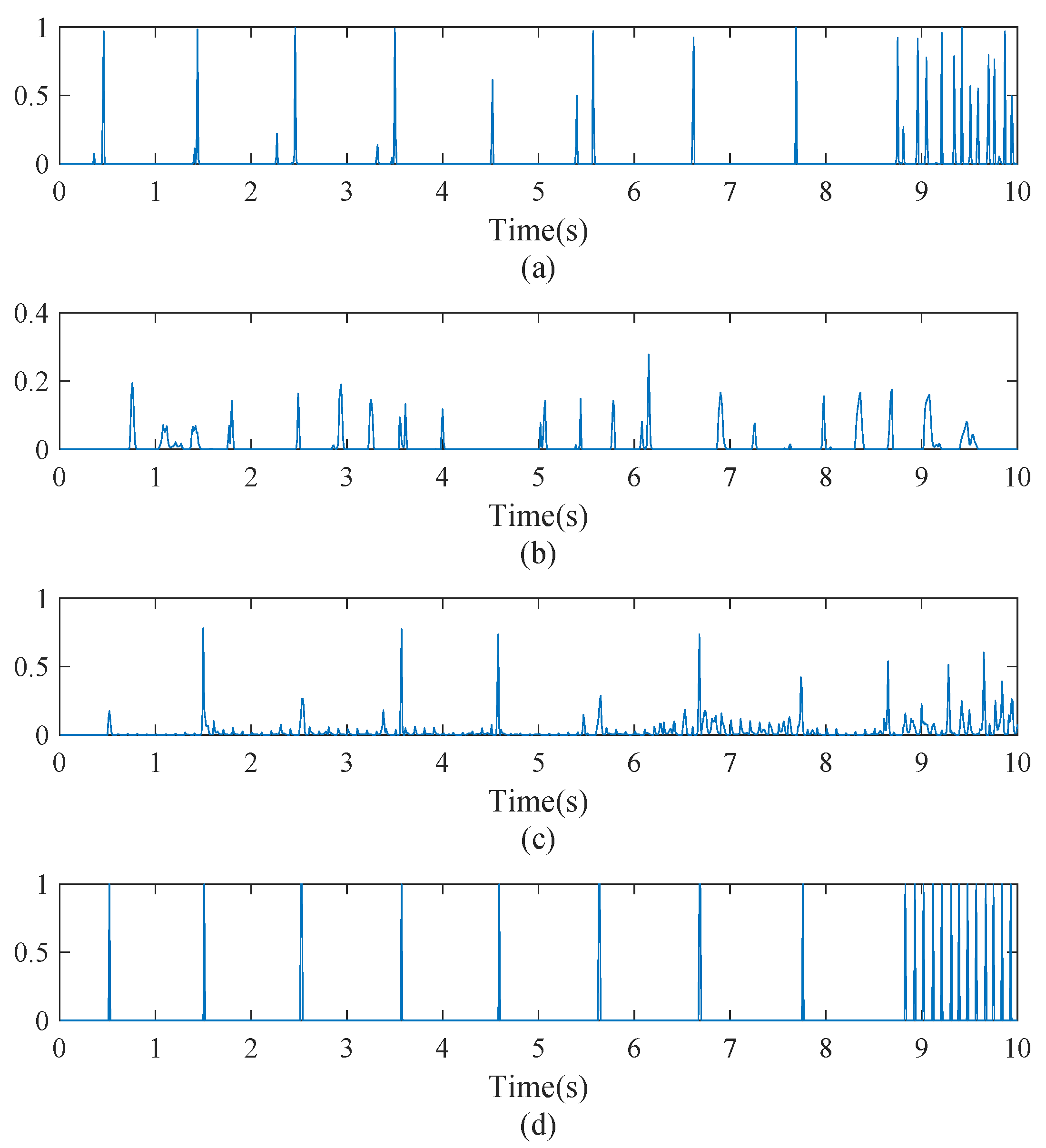
An extra stage of note verification is conducted for the specific piano, in which the spectrogram factorization improves the precision of transcription. Compared with the traditional NMF, the proposed note verification stage could save computing time and storage space to a great extent.
(3)
The proposed method achieves better performance in specific piano transcription compared to the state-of-the-art approach.
The outline of this paper is as follows. The proposed framework is described in Section 2. The transcription and comparison experiments are presented in Section 3. Finally, conclusions are drawn in Section 4.

2. Proposed Framework

The proposed transcription framework is shown in Figure 2, which comprises a note recognition module and a note verification module. In this section, we describe the two stages.

2.1. Note Recognition

Recently, convolutional learning has achieved great success in music signal processing, such as genre classification [34], artist classification [35], and chord detection [36]. In the task of AMT, CNNs have also been evaluated for onset detection and frame-based transcription, respectively. In the experiments of onset detection, Schlüter used CNNs of different architectures [37]. The results shows that a CNN with linear rectifier outperformed the state-of-the-art while requiring less manual preprocessing. Sigtia utilized a CNN to transcribe polyphonic piano music frame-by-frame, and the output was estimated pitches at each frame [21]. Although CNN yields the best performance on the frame-based metrics, an NMF method outperforms CNN on note-based metrics. So, it is promising for CNN to make use of the note onset and generate a note-based transcription. Here we train a CNN to detect onset and another CNN to estimate pitches at each detected onset.
CNNs are neural networks characterized by a convolutional structure. The convolutional layers are designed to preserve the spatial structure of the input. In each convolutional layer, a set of weights act on a fixed-size local region of the input. These weights are then repeatedly applied to the entire input to produce a feature map. After the convolution of input with shared weights, the output of the convolutional layer is obtained by adding a bias term and then applying a non-linear function. Each unit of out feature map in the convolutional layer can be computed as:
q j , m = f ( i I n N o i , n + m 1 w i , j , n + b j )
where o i , m is the mth unit of the ith input feature map, q j , m is the mth unit of the jth output feature map, w i , j , n is the nth element of the weight vector, b j is the bias term added to the jth feature map, f ( · ) is the activation function. I is the number of input feature maps, and N is the size of weight filter. A convolutional layer is often followed by a pooling layer, which subsamples each feature map. For example, the most common max pooling only retains the maximum value in non-overlapping cells. When the max pooling function is used, the pooling layer is defined as:
p j , m = max k = 1 K q j , ( m 1 ) × s + k
where K is the pooling size and s is the shift size of pooling windows. Here, p j , m is the mth unit of the jth output feature map. q j , m is the mth unit of the jth input feature map in this pooling layer, and it is also the corresponding unit of the output feature map in the last convolutional layer. Finally, the CNN ends in fully-connected layers that integrate the information of layers below. In audio signal processing, the input to the CNN is a window of feature frames centering around time t, whereas the output contains posterior probabilities of different categories at time t.
There are several motivations for applying CNNs to music transcription. Firstly, aggregating over several frames achieves better performance than processing a single frame. For example, the attack stage of notes can be modeled by applying a context window around the onset so that the onset will be detected more accurately. Secondly, the architecture of the CNN can learn features along both the time and frequency axes. CNN is proper for processing the harmonic structure in a spectrogram because of its shift invariance. Compared with deep neural network (DNN) and RNN, the weight sharing and pooling architecture leads to a reduction of parameters.
In the proposed note recognition stage, two CNNs are trained using a constant Q transform (CQT) of the music signal. The spectrogram of CQT is suited as time–frequency representation for music since its frequency bins are evenly spaced on a logarithmic axis. Additionally, the inter-harmonic spacings are constant for different pitches so that the CNN can learn pitch-invariant information. We trained a CNN of one output unit as an onset detector, giving binary labels to distinguish onsets from non-onsets. The architecture of this CNN is shown in Figure 3. The CNN takes a spectrogram slice of several frames as a single input, and each spectrogram excerpt centers on the frame to be detected. All of the spectrograms are extracted along the music signal, with a hop size of one frame. Feeding the spectrograms of the test signal to the network, we can obtain an onset activation function over time. The frame whose activation function is greater than the threshold is set to be the candidate onset.
The onset detector is followed by another CNN for multi-pitch estimation (MPE), which has the same architecture except for the output layer. Its input is a spectrogram slice centered at the onset frame. The CNN has 88 units in the output layer, corresponding the 88 pitches of piano. To make sure the multiple pitches can be estimated at the same time, all the outputs are transformed by a sigmoid function. For each training sample, the onset time is annotated accurately in advance. In the testing procedure, the input is a spectrogram slice centered at the candidate onset, which is detected by the previous CNN. A set of probabilities of 88 pitches is estimated through the network. Finally, the candidate pitches at candidate onsets are obtained by applying a threshold to the output.

2.2. Note Verification

Note verification for the specific piano is implemented through an NMF. As a frame-based approach, the traditional NMF factorises a spectrogram of a piano signal into 88 spectral bases and sparsity activations. Here the NMF only takes the candidate onsets and pitches into consideration and provides a note-wise representation. In the proposed framework, the sound to be transcribed is reconstructed by:
R t T t + T = k = 1 K W k H t T t + T
where R t T t + T is the reconstructed spectrogram of 2 T + 1 frames and t is the frame of candidate onset. W is the attack template for the specific piano, k [ 1 , K ] is the index of candidate pitches, and H t T t + T is the note activations. For the piano to be transcribed, 88 individual notes are pre-recorded and each template is obtained by computing the average spectrum over time frames. The attack template was calculated using the attack stage of each note rather than the whole duration. Note activations H t T t + T can be estimated by minimising the difference between the reconstruction R t T t + T and the original spectrogram X t T t + T . The spectrogram X t T t + T is also the input being fed to the pitch estimation CNN. Finally, we verified the candidate notes from activations. Only the candidate pitches whose peaks in the activations exceed a threshold will be identified. Meanwhile, the time when activations exceed the threshold will be set as the onset. Compared with the traditional NMF, the proposed method can save computing time and storage space to a great extent.
An illustration of note verification is shown in Figure 4. Figure 4a is a spectrogram excerpt used for traditional NMF, in which a C4 note starts at 0.14 s and ends at 0.96 s. Additionally, a C#4 note fades away before the C4 note appears, and a A3 note is played at last. Here, we only present the factorization of note C4. The templates and activations are shown in Figure 4b,c, respectively. Compared with the traditional template (solid line), the attack template (dashed line) concentrates on the percussive stage of the note and shows a different characteristic. For example, both the high-order harmonics and components between harmonics have higher amplitude in the spectrum of the attack template. In Figure 4c, the solid line is the frame-wise activations for traditional NMF, and the dashed line corresponds to the attack activations for note verification. Both curves rise rapidly at the onset time, and a note C4 can be detected using a threshold of 3.0. However, another peak appears in the curve of traditional activations at the end of note C4, and a false positive will be detected using the threshold. Therefore, the NMF using attack templates are more suitable to be applied in note verification.
In the stage of note verification, the effect of the dynamic level of templates is important. Even for a specific piano, the spectrograms of same pitch vary depending on different dynamics. Figure 5 shows the attack templates of note C4, played at three common dynamics: forte, mezzo-forte, and piano. As shown in Figure 5, there are differences between the templates of three dynamics—especially for the higher partials. In the high-frequency range, the notes of louder dynamic have richer spectral content compared to notes of softer dynamics. This indicates that the louder dynamics excite more modes in the vibration of strings than softer dynamics, which is consistent with the assumption of [30]. If we factorize a forte note using piano templates, false positives may happen because the forte note contains some spectral content which is not present in the corresponding piano template. This error will not occur when we transcribe a note using attack templates of louder dynamics.

3. Experiments

In this section, we describe the dataset used in our experiments. Then, the experimental preprocessing, parameters, and metrics are introduced. Finally, we present the results from the different experiments and analyze the performance of the proposed approach.

3.1. Dataset

The transcription experiments were conducted on the MIDI aligned piano sounds (MAPS) dataset [38]. The MAPS dataset provides piano recordings, the related aligned MIDI files, and annotated text files. The overall size of MAPS is about 60 h of audio, and it is the largest database for piano transcription. There are nine categories of recordings corresponding to different piano types and recording conditions. Seven categories of audio are produced by software piano synthesizers, while two categories of recordings are obtained from a real Yamaha Disklavier upright piano. The dataset consists of isolated notes, chords, and 30 pieces of music in each category. For music pieces, the number of concurrent notes ranges from one to nine. Each music piece lasts more than 30 s, and all 270 pieces contain 18 h of audio signal.
We aim at the transcription of the Disklavier piano, which is in category “ENSTDkCl” of the MAPS dataset. For the real piano, the recording room was a studio with dimensions equal to about 4 × 5 m. The distance between the piano and the microphones was about 50 cm. MIDI files were created beforehand and were sent to the MIDI input of the Disklavier. Then, the audio was recorded using two omnidirectional microphones.
To build a universal model independent of the real individual, we trained the CNNs using 210 music pieces of synthesized pianos in the MAPS dataset. The training set contains 460,988 notes and the overall size is about 14 h. The proposed system was evaluated on the music pieces of the Disklavier piano. In the testing set, there are 30 music pieces, and only the first 30 s of each piece was used for transcription. The testing set contains 7345 notes in total. The setting is realistic because the training set and testing set are disjoint on piano types. During the note verification, the attack templates were obtained from the isolated notes produced by the same piano.

3.2. Experimental Settings

The proposed framework takes the spectrograms of CQT as input. The audio signal was segmented with a frame length of 100 ms and a hop-size of 10 ms. The CQTs cover 88 notes of piano, and there are 36 bins per octave. Hence, a 267-dimensional CQT vector is extracted for each frame. A context window of nine frames was applied to the CQTs so that we could obtain a spectrogram slice.
In the note recognition, architectures of these two CNNs were similar (as shown in Figure 3): two convolutional layers, two pooling layers, and two fully-connected layers. These two CNNs have the same structure, except for the final fully-connected layer. For the spectrogram slices of 267 dimensions by 9 frames, the first convolutional layer with 10 filters of size 16 × 2 computes 10 feature maps of size 252 × 8 . The next layer performs max-pooling of 2 × 2 , reducing the size of maps to 126 × 4 . The second convolutional layer contains 20 filters of size 11 × 3 , which generates 20 feature maps of 116 × 2 . The max-pooling size of the second pooling layer was also set to 2 × 2 , resulting in 20 maps of 58 × 1 . The first fully-connected layer contains 256 units, and the number of units in the final layer changes with the task. In the CNN for onset detection, the final fully-connected layer has a single output unit. In the CNN for MPE, the final fully-connected layer has 88 output units. The two convolutional layers and the first fully-connected layer use the rectified linear unit (ReLU) activation function, and the final fully-connected layers use the sigmoid function. Appendix A shows more details about the CNNs.
The CNNs were trained using mini-batch gradient descent, and the size of a mini-batch was 256. The Adam algorithm [39] was also used in the training. An initial learning rate of 0.01 was decreased to 0 over 100 epochs. To prevent over-fitting, a dropout of 0.5 was applied to each network. We also used the method of early stopping, in which training was stopped if the cost (cross entropy) did not decrease for 20 epochs. The training of two CNNs was independent, whereas the CNNs were concatenated in the testing procedure. For the testing data, the first CNN estimates the candidate onset and the input of the second CNN is a spectrogram slice centered at the candidate onset.
During the note verification, we trained one attack template per pitch using the forte notes. The attack template was obtained by calculating the average of first 5-frame spectrogram followed by the onset. Each spectrum to be factorised is 267 dimension by 9 frames, and the central frame is the candidate onset detected by the first CNN.
Note-based metrics were employed to assess the performance of the proposed system [40]. A note event is regarded as right if its pitch is correct and its onset is within a ± 50 ms range of the ground truth onset. These measures are defined as:
P = N T P N T P + N F P
R = N T P N T P + N F N
F = 2 × P × R P + R
where P, R, F correspond to precision, recall, and F-measure, respectively, and N T P , N F P , and N F N are the numbers of true positives, false positives, false negatives respectively.

3.3. Results

To evaluate the performance of proposed approach comprehensively, we present the results of each step. Firstly, we analyze the performance of two CNNs, which were trained for onset detection and pitch estimation, respectively. Additionally, the performance of the proposed note recognition module was evaluated on piano transcription. At last, we compared the proposed approach with a state-of-the-art method on individual-specific transcription.

3.3.1. Onset Detection

For comparative purposes, the DNN and RNN were used for onset detection. In the training of DNN and RNN, we performed a grid search over sets of parameters to find an architecture with the best performance. The uncertain parameters of neural networks are: number of layers L { 1 , 2 , 3 , 4 } , number of hidden units H { 32 , 64 , 128 , 256 , 512 } . The hidden unit activation is a ReLU function and the output unit activation is sigmoid. In the architecture of RNN, LSTM [41] units are used, and the length of sequence was set to 10. The other parameters and methods in training are same as them in the CNN, such as dropout and early stopping.
All the results of onset detection are presented in Table 1. As shown in Table 1, the CNN performs best and the RNN outperforms DNN on all evaluation metrics. For example, the CNN yields a relative improvement of 2.84% over the RNN, and the RNN outperforms the DNN by 4.48% on F-measure. Both the CNN and RNN take a sequence of spectrums as input, which utilize the context information over time. Additionally, the spatial structure of the spectrogram is preserved by the CNN, which is useful for onset detection.
Figure 6 shows the outputs of neural networks for a music excerpt along with the corresponding ground truth. The excerpt is the first 10 s of track MAPS_MUS-bk_xmas5_ENSTDkCl. It is a typical example for transcription, and it is analyzed in each of the following experiments. In the ground truth (Figure 6d), there are two values: zero represents non-onset, and one stands for onset. We can also observe that the onset is sparse in the excerpt’s first 8.8 s, and it is dense in the last 1.2 s. As shown in Figure 6, the DNN’s output is far away from the ground truth, which cannot detect the dense onset and bring many false positives. This example explains why the DNN yields low recall and precision in Table 1. RNN and CNN are more suitable for onset detection than DNN. This is largely due to the context information over time. The evolution of a note can be modeled using the sequence information, so the false positives will not be detected in the sustain or decay stage of the note. Compared to RNN, CNN’s output is closer to the ground truth—especially for the dense onset. When two adjacent onsets have small time difference, their detection is difficult through change along the time axis. In this case, we can identify the onset using the pitch information. CNN is such a method, which learns a feature along both the time and frequency axes through its convolutional layers.

3.3.2. Multi-Pitch Estimation

The DNN and RNN were also used as comparative methods for pitch estimation. The architecture and training parameters are the same as that in onset detection, except for the final layer. Each net has 88 units in the output layer, and the output unit activation is sigmoid. In the training and evaluation, all onset time was determined accurately in advance, and the pitch estimation was carried out at each onset.
The results of MPE are shown in Table 2. As shown in Table 2, the CNN outperformed other nets on all evaluation metrics. For example, the CNN yielded a relative improvement of 24.61% over the DNN and outperformed RNN by 15.91% on note-based F-measure. This is largely because the CNN can learn pitch-invariant features from the frames around the onset. We can also observe that the RNN outperformed the DNN on precision and F-measure, which indicates that the context information is helpful in pitch estimation. Therefore, the advantage of CNN is significant in the subtask of onset detection and MPE.
Figure 7 shows the graphical representation of the outputs of neural networks for the music excerpt along with the corresponding ground truth piano roll. As shown in the ground truth (Figure 7d), the pitch estimation of this excerpt is challenging. The polyphony at each time instant is four in the excerpt’s first 8.8 s, and the overlapping is serious. Additionally, the notes are much shorter in the excerpt’s last 1.2 s. Compared to the posteriograms of CNN and RNN, DNN estimated more pitches, where many of them were false positives. This is because DNN’s topology is simple and its input is just the spectrum at onset. Utilizing the note sequence information in piano music, RNN produced a higher-precision output. However, RNN’s output seemed to be a result of monophonic pitch estimation, which yielded many false negatives and corresponded to low recall. In general, the CNN’s output was much closer to the ground truth than DNN and RNN. Unlike RNN’s input, the context information of CNN’s input is from several frames around each onset. CNN can model the attack stage of each pitch through this information, such that the MPE at onset is more accurate. There are also some octave errors which require further effort in the CNN’s posteriogram. For example, the MIDI pitch of 46 (about 116.54 Hz) was estimated to be MIDI pitch 58 (about 233.08 Hz) at the eighth onset.

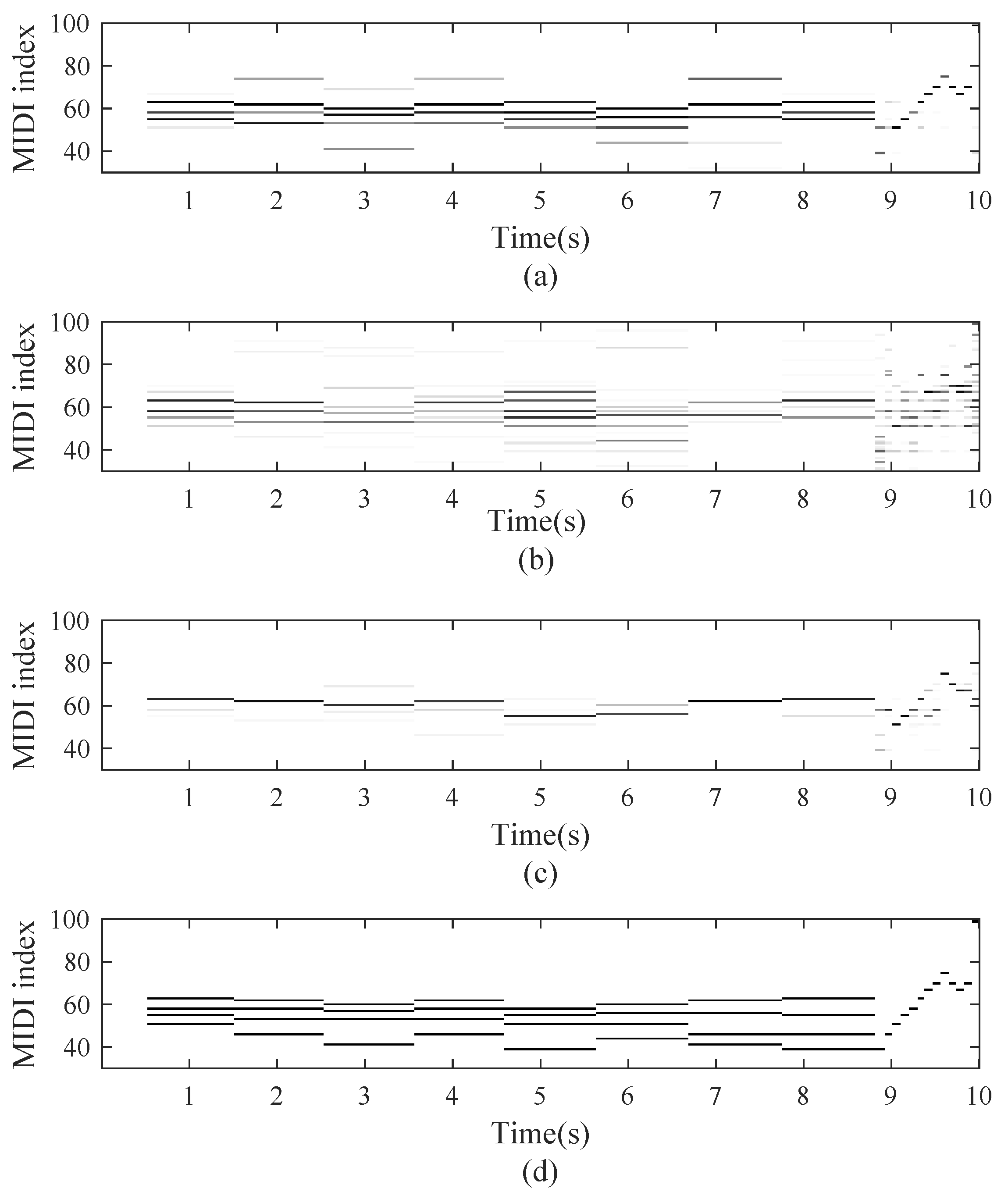
3.3.3. Note Recognition

To evaluate the performance of the proposed note recognition stage which contains two CNNs, another CNN system was used for comparison [21]. The system contained only a single CNN, which transcribes music frame-by-frame and returns a list of notes with pitches and onset. This system will be referred to as Sigtia. Actually, the note recognition stage can be treated as a piano transcription system, which takes no account of the individual to be transcribed. To make a comprehensive comparison, two state-of-the-art transcription methods were also used. Both were submitted to MIREX and evaluated in the task of piano tracking. Benetos’s method uses a variable-Q transform representation as input and employs probabilistic latent component analysis in transcription [42]. Troxel’s system is based on Microsoft’s ResNet, and it has achieved the best performance in MIREX. For Sigtia’s method, we trained a CNN using parameters he described in [21]. We have access to the code of Benetos’s method, and the second baseline system was implemented by the code. For Troxel’s system, the results were obtained from the transcription software named AnthemScore [43].
All of the note-based results of transcription are presented in Table 3. In general, the performance of the proposed note recognition stage is acceptable. Among these four methods, Benetos’ approach performed the worst on each evaluation measure. This is because Benetos’ model is trained for multiple instruments instead of piano, and the pre-shifted templates are not helpful for piano transcription. The proposed note recognition module outperformed Sigtia’s method on all evaluation metrics, which indicates that two independent CNNs are superior to a single one in AMT. Troxel’s method yielded the best performance, and it outperformed us by only 0.14% on F-measure. On the metrics of precision, our proposed note recognition stage was inferior to Troxel’s system. Therefore, we can use a note verification stage to reduce the false positive notes and improve the precision of transcription.
Figure 8 shows the transcription of the MAPS_MUS-bk_xmas5_ENSTDkCl excerpt using the top two systems in Table 3. The corresponding ground truth has been shown in Figure 7d. Compared with the ground truth, the false positive notes are marked using red crosses and the false negative notes are marked using a blue dashed line. We can observe that the onset of notes in Figure 8a are detected more accurately than that in Figure 8b. This can be attributed to the CNN for onset detection in our system. In the excerpt’s first 8.8 s, the transcription result of Troxel’s system is better than that of our two consecutive CNNs. There are eight false negative errors and five false positive errors in Figure 8a. Correspondingly, there are only three false negative notes and two false positive notes in Figure 8b. One solution to reduce the false negative errors is to apply a small threshold to the output of the second CNN. This will bring more false positive notes, so an additional note verification stage is necessary. In the excerpt’s last 1.2 s, the performance of our note recognition stage was much better than Troxel’s system. As the duration of notes here are short, the accurate onset is essential for transcribing them. This also indicates the advantage of our CNNs on short-note transcription.

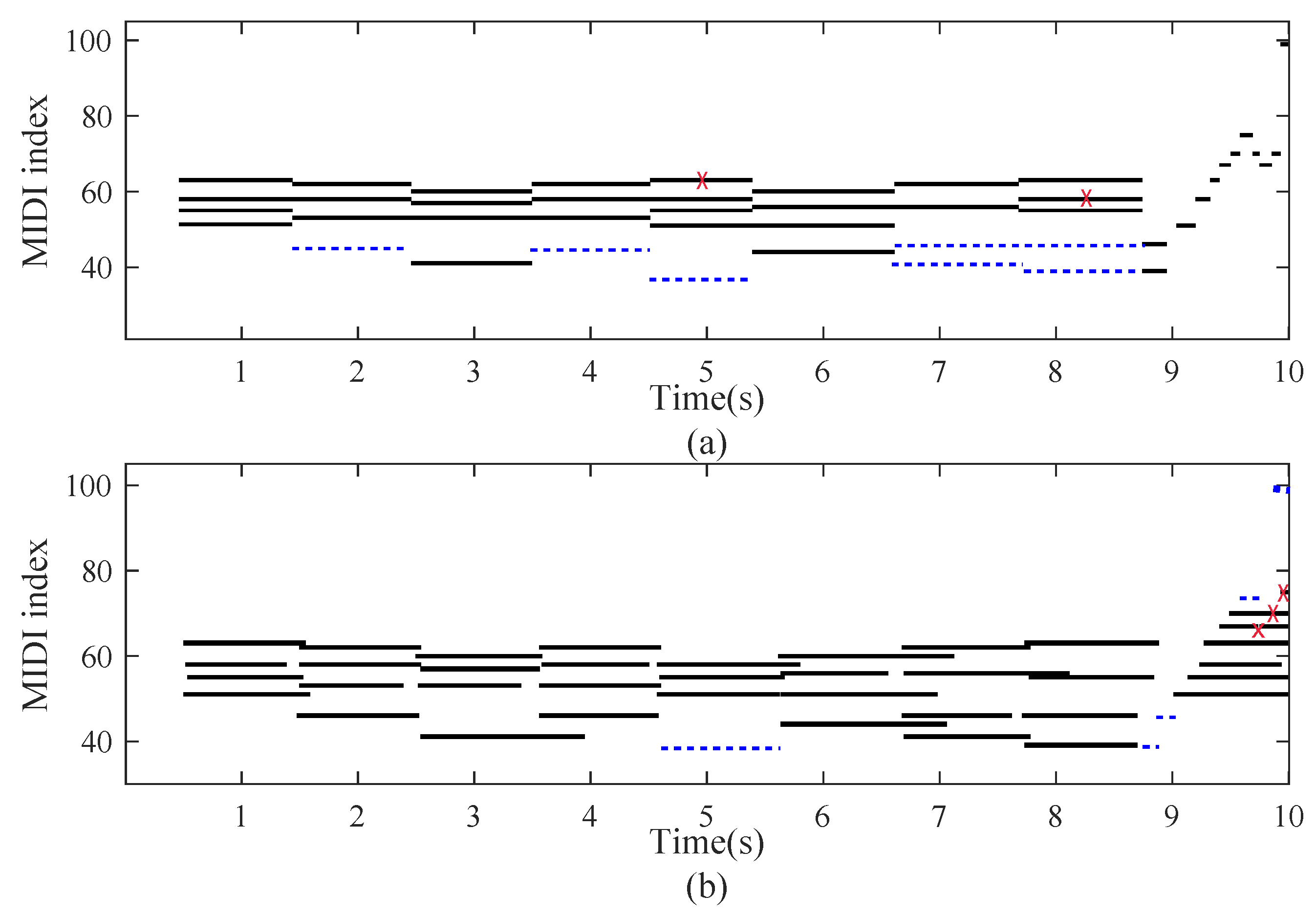
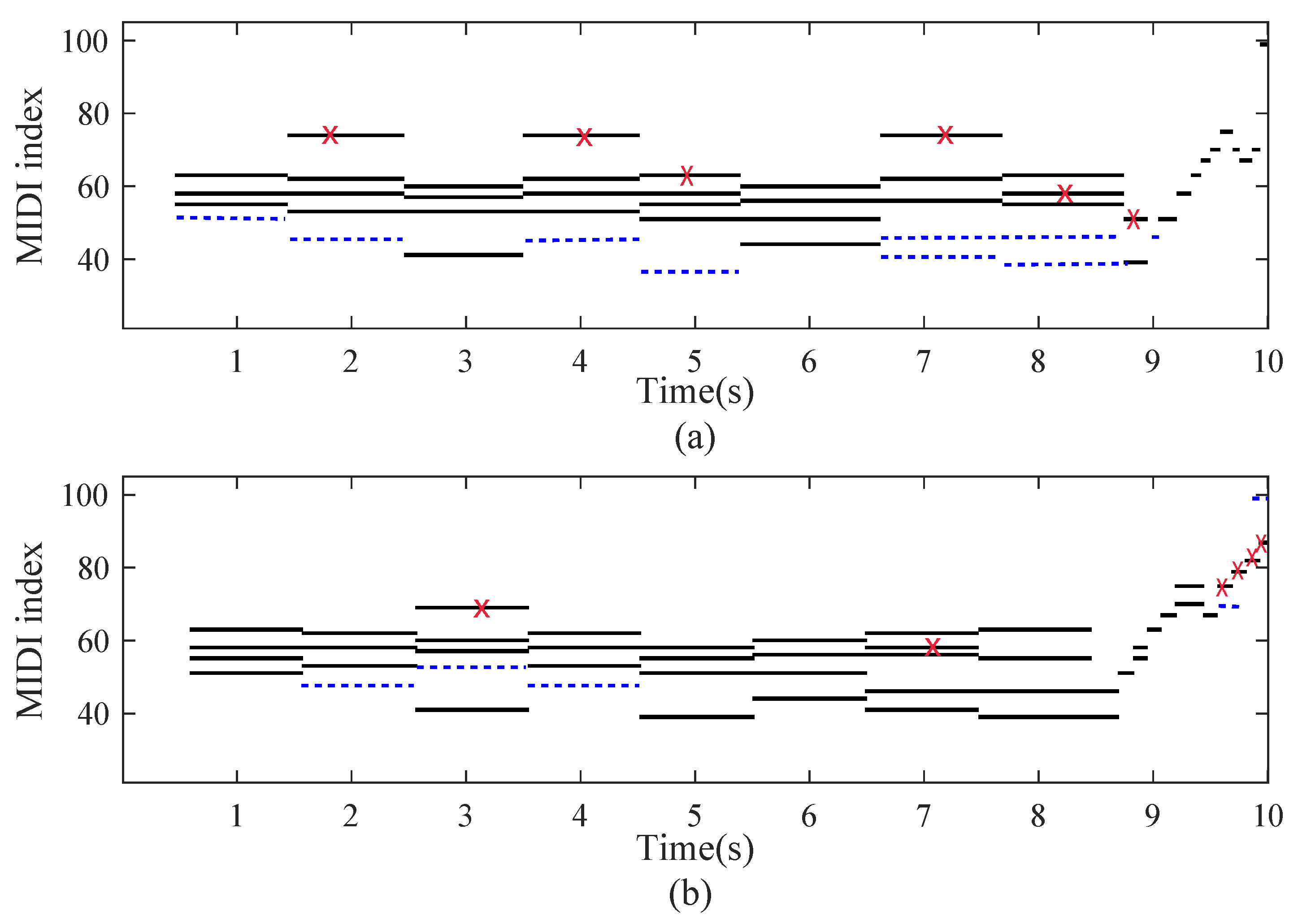
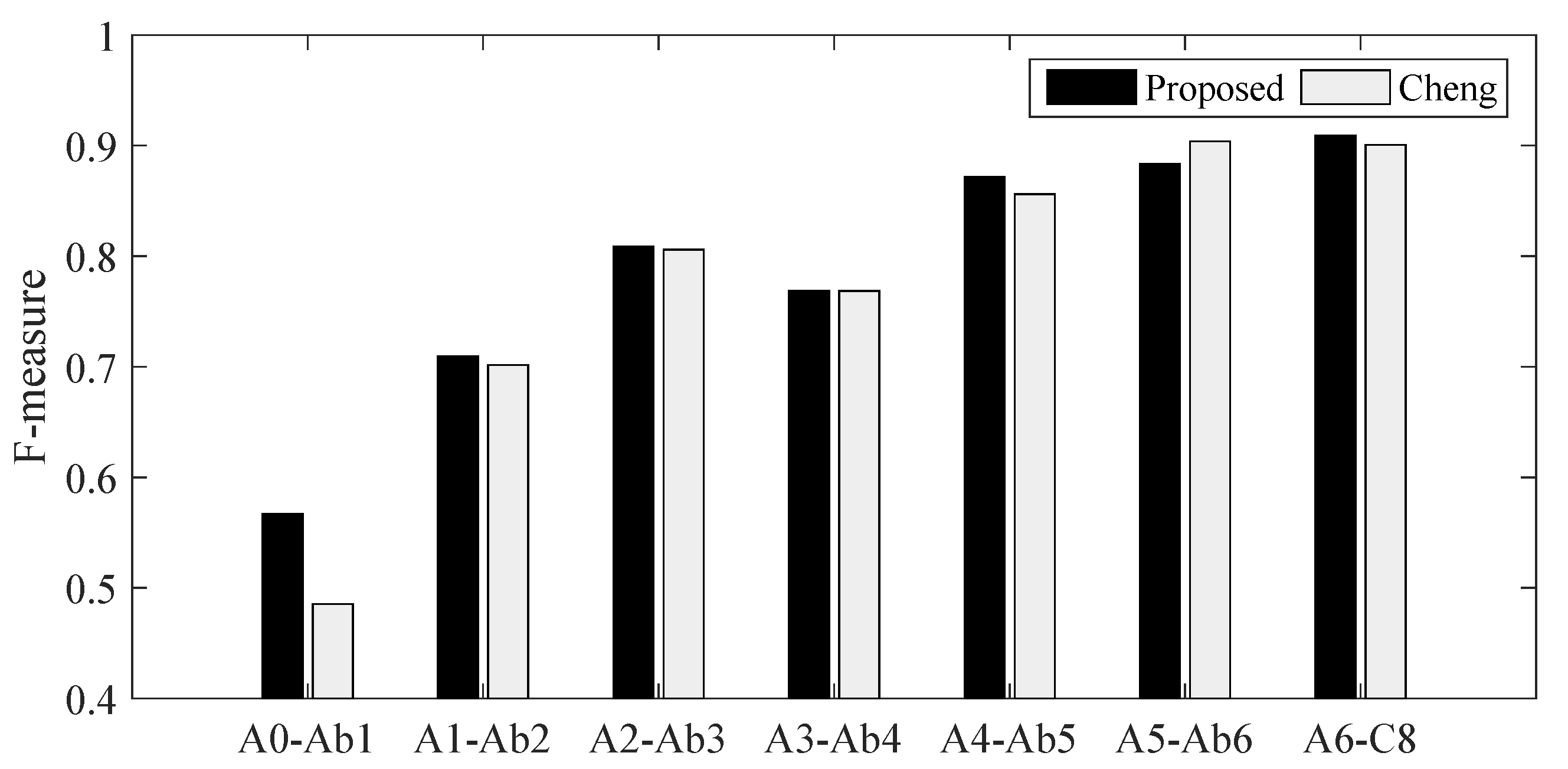
3.3.4. Transcription for Specific Piano

In our proposed framework, the individual-specific transcription is conducted by feeding the output of note recognition into a note verification stage. For comparative purposes, two transcription systems were used to evaluate the performance of the proposed method. The first comparative approach was proposed by Cheng, which is the current state-of-the-art specific piano transcription method [32]. Cheng’s method is implemented using a sparse NMF in AMT, and all the templates are extracted using the notes from "ENSTDkCl" of MAPS. Considering that the CNNs have shown advantages in the note recognition stage, the second comparative approach is based on them. Adding the specific individual’s data to the training set, we got two adapted CNNs. To make a fair comparison, the newly-added training samples were isolated notes produced by the same piano.
The transcription results are shown in Table 4, and the proposed method performed best in general. Although they are based on the same note recognition module, the proposed system outperformed the adapted CNNs on all evaluation metrics. This illustrates the benefits of note verification. Another reason is that the CNNs cannot learn enough information about the specific individual through these limited isolated notes—especially the information of polyphony. The proposed system outperformed Cheng’s system in terms of recall and F-measure. Our proposed method estimated 5511 notes correctly, whereas the number of true positive notes was 5421 for Cheng’s method. This can be attributed to the use of note recognition, which achieved significant performance on recall through CNNs. Meanwhile, the preliminary results led to a limitation of note verification. Both the proposed method and Cheng’s method achieved better performance than the adapted CNN on all evaluation metrics. One of the reasons may be that both of them use the templates of attack during the NMF.
In general, all of the specific piano transcription systems in Table 4 perform better than universal systems in Table 3. We can conclude that making use of the information of specific individual is promising in AMT. Compared with results in Table 3, The proposed system performed better on the metrics of precision and F-measure when the note verification stage was applied. Therefore, the effectiveness of note verification is validated again.
The results of the proposed method and the state-of-the-art method are compared concretely. Figure 9 shows the F-measure obtained by our proposed and Cheng’s methods, which is along the different octaves of a piano. As shown in Figure 9, our proposed method outperformed Cheng’s method for six octaves, except for the A5-Ab6 octave. Cheng’s method achieved an F-measure of 0.4854 for A0-Ab1, which shows its poor performance in the transcription of low-pitch notes. The proposed method showed a more balanced result, with an F-measure of 0.5672 for the first octave. In general, the F-measure increased approximately along the increase of octaves for the two methods. This suggests the limitation of the time-domain approach, which brings a time–frequency resolution trade-off.
Figure 10 shows the specific piano transcription of the MAPS_MUS-bk_xmas5_ENSTDkCl excerpt, which was produced by our proposed framework and Cheng’s system. Compared with the ground truth in Figure 7d, the false positive notes are marked using red crosses, and the false negative notes are marked using a blue dashed line. The contrast between Figure 8a and Figure 10a indicates that the note verification can improve the precision of transcription. As shown in Figure 10, Cheng’s method estimated more correct pitches than our proposed method in the excerpt’s first 8.8 s. This is due to a limitation in our proposed system. Although the note verification conducted on candidate notes can save computing time and storage space, it is limited because the candidate set is not complete. In the excerpt’s last 1.2 s, our system yielded a better performance than Cheng’s system. This indicates the advantage of our note recognition stage, which is good at transcribing short notes. Another reason is that modeling both the attack and decay stages in short duration is difficult for Cheng’s system.

4. Conclusions

We present a two-stage framework for note-level polyphonic piano music transcription, which comprises a note recognition stage and a note verification stage. In the note recognition, one CNN is trained for onset detection and another is trained for pitch estimation at each onset. To our knowledge, the combination of two CNNs has not been attempted before for AMT. The note verification for the specific piano is implemented using NMF. The factorization is conducted in the time slice around candidate onset, which only uses attack templates of the candidate pitches. Our experiments are carried out on the MAPS database and the performance of each module is discussed. The experiments demonstrate that CNN performs better than other types of neural networks in the subtasks of onset detection and pitch estimation, and the connection of two CNNs outperforms a single CNN in note recognition. We also observe that the performance of transcription is improved significantly when note verification is applied to the system, and our proposed system performs better than state-of-the-art systems in specific piano transcription.
There are some limitations of the proposed system. As the biggest dataset for piano AMT, the MAPS has only 270 solo pieces. So, the data may be not enough for training CNNs. Although training data and testing data are from synthesized pianos and a real piano, respectively, they contain overlaps in music pieces. The limited data and piece-dependent scheme led the CNNs to overfit. For the real pieces in the testing dataset, the recording environment was quiet and the distance between the piano and microphones was close. Therefore, one future research direction is to discuss whether the proposed method is robust to noise and reverberation. Additionally, the proposed method cannot estimate note offsets or loudness, which will be another research direction in the future.

Acknowledgments

This work is partially supported by the National Natural Science Foundation of China (Nos. 11461141004, 61271426, U1536117, 11504406, 11590770-4), the Strategic Priority Research Program of the Chinese Academy of Sciences (Nos. XDA06030100, XDA06030500, XDA06040603), the National 863 Program (No. 2015AA016306) and the National 973 Program (No. 2013CB329302).

Author Contributions

Qi Wang and Ruohua Zhou conceived of and designed the experiments; Qi Wang performed the experiments; Qi Wang and Ruohua Zhou analyzed the data; Yonghong Yan contributed analysis tools; Qi Wang wrote the paper.

Conflicts of Interest

The authors declare no conflict of interest.

Appendix A

#Builds the CNN. The code is based on the open source software library-TensorFlow.
import tensorflow as tf
 
def inference(images0):
 """Build the CNN model.
 Args: images0: Images placeholder, from inputs().
 Returns: sigmoid_linear: Output tensor with the computed probabilities.
 """
 images=tf.reshape(images0, [-1,267,9,1])
 
 # conv1
 with tf.variable_scope(’conv1’) as scope:
  weights = tf.Variable(tf.truncated_normal([16,2,1,10],stddev=0.1))
  conv = tf.nn.conv2d(images, weights, [1,1,1,1],padding=’VALID’)
  biases = tf.Variable(tf.constant(0.1,shape=[10]))
  pre_activation = tf.nn.bias_add(conv, biases)
  conv1 = tf.nn.relu(pre_activation, name=scope.name)
 
 # pool1
 pool1 = tf.nn.max_pool(conv1, ksize=[1, 2, 2, 1], strides=[1, 2, 2, 1], padding=’SAME’, name=’pool1’)
 
 # conv2
 with tf.variable_scope(’conv2’) as scope:
  weights = tf.Variable(tf.truncated_normal([11,3,10,20],stddev=0.1))
  conv = tf.nn.conv2d(pool1, weights, [1, 1, 1, 1], padding=’VALID’)
  biases = tf.Variable(tf.constant(0.1,shape=[20]))
  pre_activation = tf.nn.bias_add(conv, biases)
  conv2 = tf.nn.relu(pre_activation, name=scope.name)
 
 # pool2
 pool2 = tf.nn.max_pool(conv2, ksize=[1, 2, 2, 1], strides=[1, 2, 2, 1], padding=’SAME’, name=’pool2’)
 
 # fully-connected1
 with tf.variable_scope(’fully-connected1’) as scope:
  reshape = tf.reshape(pool2, [-1,58*1*20])
  weights = tf.Variable(tf.truncated_normal([58*1*20,256],stddev=0.1))
  biases = tf.Variable(tf.constant(0.1,shape=[256]))
  local = tf.nn.relu(tf.matmul(reshape, weights) + biases, name=scope.name)
 
 # fully-connected2
 with tf.variable_scope(’fully-connected2’) as scope:
  #dropout
  local3_drop =tf.nn.dropout(local, 0.5)
  weights = tf.Variable(tf.truncated_normal([256,num_classes],stddev=0.1))
  biases = tf.Variable(tf.constant(0.1,shape=[num_classes]))
  sigmoid_linear = tf.nn.sigmoid(tf.matmul(local3_drop, weights) + biases, name=scope.name)
 return sigmoid_linear
 
def loss(logits, labels):
 """Calculates the loss from the logits and the labels.
 Args:
 logits: Logits from inference(), float - [batch_size, num_classes].
 labels: Labels tensor, int32 - [batch_size, num_classes].
 Returns: cross_entropy: Loss tensor of type float.
 """
 cross_entropy = -tf.reduce_sum(labels*tf.log(logits+1e-10)+(1-labels)*tf.log(1-logits+1e-10))
 return cross_entropy
 
def evaluation(logits, labels, threshold):
 """Evaluate the quality of the logits at predicting the label.
 Args:
 logits: Logits from inference(), float - [batch_size, num_classes].
 labels: Labels tensor, int32 - [batch_size, num_classes].
 threshold: Threshold applied to the logits.
 Returns: accuracy: Compute precision of predicting.
 """
 pred=tf.cast(tf.greater(logits, threshold),"float")
 correct_prediction = tf.cast(tf.equal(pred, labels), "float")
 accuracy = tf.reduce_mean(correct_prediction)
 return accuracy
 
def training(loss, learning_rate):
 """Sets up the training Ops.
 Creates an optimizer and applies the gradients to all trainable variables.
 Args:
 loss: Loss tensor, from loss().
 learning_rate: The learning rate to use for gradient descent.
 Returns: train_op: The Op for training.
 """
 # Create the gradient descent optimizer with the given learning rate.
 optimizer = tf.train.AdamOptimizer(learning_rate)
 # Use the optimizer to apply the gradients that minimize the loss
 train_op = optimizer.minimize(loss)
 return train_op

References

  1. Moorer, J.A. On the transcription of musical sound by computer. Comput. Music J. 1977, 1, 32–38. [Google Scholar]
  2. Piszczalski, M.; Galler, B.A. Automatic music transcription. Comput. Music J. 1977, 1, 24–31. [Google Scholar]
  3. Klapuri, A. Introduction to music transcription. In Signal Processing Methods for Music Transcription; Springer: Boston, MA, USA, 2006; pp. 3–20. [Google Scholar]
  4. Cogliati, A.; Duan, Z.; Wohlberg, B. Piano transcription with convolutional sparse lateral inhibition. IEEE Signal Process. Lett. 2017, 24, 392–396. [Google Scholar] [CrossRef]
  5. Benetos, E.; Dixon, S.; Giannoulis, D.; Kirchhoff, H.; Klapuri, A. Automatic music transcription: Challenges and future directions. J. Intell. Inf. Syst. 2013, 41, 407–434. [Google Scholar] [CrossRef]
  6. Klapuri, A.P. Multiple fundamental frequency estimation based on harmonicity and spectral smoothness. IEEE Trans. Speech Audio Process. 2003, 11, 804–816. [Google Scholar] [CrossRef]
  7. Pertusa, A.; Inesta, J.M. Multiple fundamental frequency estimation using Gaussian smoothness. In Proceedings of the IEEE International Conference on Acoustics, Speech and Signal Processing (ICASSP), Las Vegas, NV, USA, 31 March–4 April 2008; pp. 105–108. [Google Scholar]
  8. Brown, J.C. Calculation of a constant Q spectral transform. J. Acoust. Soc. Am. 1991, 89, 425–434. [Google Scholar] [CrossRef]
  9. Zhou, R.; Reiss, J.D. A real-time polyphonic music transcription system. In Proceedings of the 4th Music Information Retrieval Evaluation eXchange (MIREX), Philadelphia, PA, USA, 14–18 September 2008. [Google Scholar]
  10. Dressler, K. Multiple fundamental frequency extraction for MIREX 2012. In Proceedings of the 8th Music Information Retrieval Evaluation eXchange (MIREX), Porto, Portugal, 8–12 October 2012. [Google Scholar]
  11. Smaragdis, P.; Brown, J.C. Non-negative matrix factorization for polyphonic music transcription. In Proceedings of the IEEE Workshop on Applications of Signal Processing to Audio and Acoustics, New Paltz, NY, USA, 19–22 October 2003; pp. 177–180. [Google Scholar]
  12. Smaragdis, P.; Raj, B.; Shashanka, M. A probabilistic latent variable model for acoustic modeling. Adv. Models Acoust. Process. 2006, 148, 1–8. [Google Scholar]
  13. Benetos, E.; Dixon, S. A shift-invariant latent variable model for automatic music transcription. Comput. Music J. 2012, 36, 81–94. [Google Scholar] [CrossRef]
  14. Nam, J.; Ngiam, J.; Lee, H.; Slaney, M. A classification-based polyphonic piano transcription approach using learned feature representations. In Proceedings of the International Society for Music Information Retrieval Conference (ISMIR), Miami, FL, USA, 24–28 October 2011; pp. 175–180. [Google Scholar]
  15. Sigtia, S.; Benetos, E.; Boulanger-Lewandowski, N.; Weyde, T.; Garcez, A.S.D.; Dixon, S. A hybrid recurrent neural network for music transcription. In Proceedings of the 2015 IEEE International Conference on Acoustics, Speech and Signal Processing (ICASSP), Brisbane, QLD, Australia, 19–24 April 2015; pp. 2061–2065. [Google Scholar]
  16. Kelz, R.; Widmer, G. An experimental analysis of the entanglement problem in neural-network-based music transcription systems. In Proceedings of the AES Conference on Semantic Audio, Erlangen, Germany, 22–24 June 2017. [Google Scholar]
  17. Berg-Kirkpatrick, T.; Andreas, J.; Klein, D. Unsupervised transcription of piano music. In Proceedings of the International Conference on Neural Information Processing Systems (NIPS), Montreal, QC, Canada, 8–13 Demcember 2014; pp. 1538–1546. [Google Scholar]
  18. Ewert, S.; Plumbley, M.D.; Sandler, M. A dynamic programming variant of non-negative matrix deconvolution for the transcription of struck string instruments. In Proceedings of the IEEE International Conference on Acoustics, Speech and Signal Processing (ICASSP), Brisbane, QLD, Australia, 19–24 April 2015; pp. 569–573. [Google Scholar]
  19. Kameoka, H.; Nishimoto, T.; Sagayama, S. A multipitch analyzer based on harmonic temporal structured clustering. IEEE Trans. Audio Speech Lang. Process. 2007, 15, 982–994. [Google Scholar] [CrossRef]
  20. Böck, S.; Schedl, M. Polyphonic piano note transcription with recurrent neural networks. In Proceedings of the IEEE International Conference on Acoustics, Speech and Signal Processing (ICASSP), Kyoto, Japan, 25–30 March 2012; pp. 121–124. [Google Scholar]
  21. Sigtia, S.; Benetos, E.; Dixon, S. An end-to-end neural network for polyphonic piano music transcription. IEEE/ACM Trans. Audio Speech Lang. Process. 2016, 24, 927–939. [Google Scholar] [CrossRef]
  22. Marolt, M. A connectionist approach to automatic transcription of polyphonic piano music. IEEE Trans. Multimed. 2004, 6, 439–449. [Google Scholar] [CrossRef]
  23. Costantini, G.; Perfetti, R.; Todisco, M. Event based transcription system for polyphonic piano music. Signal Process. 2009, 89, 1798–1811. [Google Scholar] [CrossRef]
  24. Barbancho, I.; de la Bandera, C.; Barbancho, A.M.; Tardon, L.J. Transcription and expressiveness detection system for violin music. In Proceedings of the IEEE International Conference on Acoustics, Speech and Signal Processing (ICASSP), Taipei, Taiwan, 19–24 April 2009; pp. 189–192. [Google Scholar]
  25. Marolt, M. Automatic transcription of bell chiming recordings. IEEE Trans. Audio Speech Lang. Process. 2012, 20, 844–853. [Google Scholar] [CrossRef]
  26. Barbancho, A.M.; Klapuri, A.; Tardón, L.J.; Barbancho, I. Automatic transcription of guitar chords and fingering from audio. IEEE Trans. Audio Speech Lang. Process. 2012, 20, 915–921. [Google Scholar] [CrossRef]
  27. Wan, Y.; Wang, X.; Zhou, R.; Yan, Y. Automatic Piano Music Transcription Using Audio-Visual Features. Chin. J. Electron. 2015, 24, 596–603. [Google Scholar] [CrossRef]
  28. 2016: Multiple Fundamental Frequency Estimation Tracking Results—MIREX Dataset. Available online: http://www.music-ir.org/mirex/wiki/2016:Multiple_Fundamental_Frequency_Estimation_%26_ Tracking_Results_-_MIREX_Dataset (accessed on 15 October 2016).
  29. Cogliati, A.; Duan, Z. Piano music transcription modeling note temporal evolution. In Proceedings of the IEEE International Conference on Acoustics, Speech and Signal Processing (ICASSP), Brisbane, QLD, Australia, 19–24 April 2015; pp. 429–433. [Google Scholar]
  30. Cogliati, A.; Duan, Z.; Wohlberg, B. Context-dependent piano music transcription with convolutional sparse coding. IEEE/ACM Trans. Audio Speech Lang. Process. 2016, 24, 2218–2230. [Google Scholar] [CrossRef]
  31. Ewert, S.; Sandler, M. Piano transcription in the studio using an extensible alternating directions framework. IEEE/ACM Trans. Audio Speech Lang. Process. 2016, 24, 1983–1997. [Google Scholar] [CrossRef]
  32. Cheng, T.; Mauch, M.; Benetos, E.; Dixon, S. An attack/decay model for piano transcription. In Proceedings of the International Society for Music Information Retrieval Conference (ISMIR), New York, NY, USA, 7–11 August 2016. [Google Scholar]
  33. Gao, L.; Su, L.; Yang, Y.H.; Lee, T. Polyphonic piano note transcription with non-negative matrix factorization of differential spectrogram. In Proceedings of the IEEE International Conference on Acoustics, Speech and Signal Processing (ICASSP), New Orleans, LA, USA, 5–9 March 2017; pp. 291–295. [Google Scholar]
  34. Li, T.L.; Chan, A.B.; Chun, A. Automatic musical pattern feature extraction using convolutional neural network. In Proceedings of the International Multi Conference of Engineers and Computer Scientists, Hongkong, China, 17–19 March 2010. [Google Scholar]
  35. Dieleman, S.; Brakel, P.; Schrauwen, B. Audio-based music classification with a pretrained convolutional network. In Proceedings of the International Society for Music Information Retrieval Conference (ISMIR), Miami, FL, USA, 24–28 October 2011; pp. 669–674. [Google Scholar]
  36. Humphrey, E.J.; Bello, J.P. Rethinking automatic chord recognition with convolutional neural networks. In Proceedings of the International Conference on Machine Learning and Applications (ICMLA), Boca Raton, FL, USA, 12–15 December 2012; Volume 2, pp. 357–362. [Google Scholar]
  37. Schluter, J.; Bock, S. Improved musical onset detection with convolutional neural networks. In Proceedings of the IEEE International Conference on Acoustics, Speech and Signal Processing (ICASSP), Florence, Italy, 4–9 May 2014; pp. 6979–6983. [Google Scholar]
  38. Emiya, V.; Badeau, R.; David, B. Multipitch estimation of piano sounds using a new probabilistic spectral smoothness principle. IEEE Trans. Audio Speech Lang. Process. 2010, 18, 1643–1654. [Google Scholar] [CrossRef]
  39. Kingma, D.; Ba, J. Adam: A method for stochastic optimization. arXiv, 2014; arXiv:1412.6980. [Google Scholar]
  40. Bay, M.; Ehmann, A.F.; Downie, J.S. Evaluation of Multiple-F0 Estimation and Tracking Systems. In Proceedings of the International Society for Music Information Retrieval Conference (ISMIR), Kobe, Japan, 26–30 October 2009; pp. 315–320. [Google Scholar]
  41. Eyben, F.; Böck, S.; Schuller, B.W.; Graves, A. Universal Onset Detection with Bidirectional Long Short-Term Memory Neural Networks. In Proceedings of the International Society for Music Information Retrieval Conference (ISMIR), Utrecht, The Netherlands, 9–13 August 2010; pp. 589–594. [Google Scholar]
  42. Benetos, E.; Weyde, T. An efficient temporally-constrained probabilistic model for multiple-instrument music transcription. In Proceedings of the International Society for Music Information Retrieval Conference (ISMIR), Malaga, Spain, 20–26 October 2015. [Google Scholar]
  43. Troxel, D. Automatic Music Transcription Software. Available online: https://www.lunaverus.com/ (accessed on 9 December 2016).
Figure 1. The 2007–2016 annual best results for piano transcription in MIREX (Music Information Retrieval Evaluation eXchange).
Applsci 07 00901 g001
Figure 2. Diagram for the proposed framework. CNN: convolutional neural network; NMF: non-negative matrix factorization.
Applsci 07 00901 g002
Figure 3. CNN architecture for onset detection.
Applsci 07 00901 g003
Figure 4. An illustration of note verification: (a) a spectrogram excerpt used for NMF; (b) the attack templates and traditional templates; (c) the attack activations and traditional activations in NMF.
Applsci 07 00901 g004
Figure 5. Attack templates of note C4 played at three dynamics: forte, mezzo-forte, and piano.
Applsci 07 00901 g005
Figure 6. Results of onset detection: (ac) the output of CNN, DNN, and RNN, respectively; (d) the corresponding ground truth.
Applsci 07 00901 g006
Figure 7. Results of multi-pitch estimation (MPE): (ac) the output of CNN, DNN, and RNN, respectively; (d) the corresponding ground truth piano roll representation.
Applsci 07 00901 g007
Figure 8. Results of piano transcription: (a) the transcription produced by CNNs in our proposed framwork; and (b) the transcription produced by Troxel’s system.
Applsci 07 00901 g008
Figure 9. F-measure per octave achieved by our proposed system and Cheng’s system.
Applsci 07 00901 g009
Figure 10. Results of specific piano transcription: (a) the transcription of our proposed system and (b) the transcription of Cheng’s system.
Applsci 07 00901 g010
Table 1. Performance on onset detection using different neural networks. DNN: deep neural network; RNN: recurrent neural network.
MethodRecallPrecisionF-Measure
CNN0.97310.95900.9660
DNN0.93190.86830.8990
RNN0.95300.92590.9393
Table 2. Performance on pitch estimation using different neural networks.
MethodRecallPrecisionF-Measure
CNN0.78100.83190.8056
DNN0.62230.67270.6465
RNN0.60200.82210.6950
Table 3. Performance on piano transcription.
MethodRecallPrecisionF-Measure
CNNs0.75240.85930.8023
Sigtia0.67860.80230.7353
Benetos0.58570.63050.6073
Troxel0.74770.86870.8037
Table 4. Performance comparison on specific piano transcription.
MethodRecallPrecisionF-Measure
Proposed0.75030.90390.8200
Cheng0.73810.90700.8139
Adapted CNNs0.74580.87920.8070

