FOG De-Noising Algorithm Based on Augmented Nonlinear Differentiator and Singular Spectrum Analysis

Abstract

A novel algorithm based on singular spectrum analysis (SSA) and augmented nonlinear differentiator (AND) for extracting the useful signal from a noisy measurement of fiber optic gyroscope (FOG) is proposed in this paper. As a novel type of tracking differentiator, augmented nonlinear differentiator (AND) has the advantages of dynamical performance and noise-attenuation ability. However, there is a contradiction in AND, i.e., selecting a larger acceleration factor may cause faster convergence but bad random noise reduction, whereas selecting a smaller acceleration factor may lead to signal delay but effective random noise reduction. To overcome the contradiction of AND, multi-scale transformation is introduced. Firstly, the noisy signal is decomposed into components by SSA, and the correlation coefficients between each component and original signal are calculated, then the component with biggest correlation coefficient is reserved and other components are filtered by AND with designed selection criterion of acceleration factor, finally the de-noising result is obtained after reconstruction process. There are mainly two prominent advantages of the proposed SSA-AND algorithm: (i) Compared to traditional tracking differentiators, better de-noising ability can be achieved without signal delay; and (ii) compared to other widely used hybrid de-noising methods based on multi-scale transformation, a parameter determination method is given based on the correlation coefficient of each decomposed component, which improves the reliability of the proposed algorithm.

1. Introduction

Fiber optic gyroscopes (FOGs) are rotation sensors. By using optic wave information, FOGs can detect the phase shift induced by the so-called Sagnac effect [1]. FOGs have already been widely used in industrial and military applications due to the advantages of long life, simple structure, dynamic range and short start-up time.

The precision of FOGs output signal would be degraded due to errors. There are two types of error, which are deterministic error and stochastic error [2,3]. Deterministic errors are caused by bias, misalignment, and scale factors, which can be reduced by appropriate calibration methods. The stochastic errors are caused by environmental temperature variations, imperfect fabrication, and other electronic equipment interference, which mainly consisted by temperature drift and random noise. The drift can be compensated by establishing a temperature model. However, the temperature drift is submerged in noise, therefore it is necessary to reduce the noise at first. Many studies have been explored to cancel out the random noise to improve the precision of temperature drift modeling and compensation. Multi-scale transformation method is a widely used technique for FOG de-noising, such as wavelet-based techniques [4,5], mode decomposition-based techniques [6,7,8], and singular spectrum analysis (SSA) [9,10]. By using multi-scale transformation methods, the signal can be decomposed from time-domain into frequency-domain, and then the high frequency noise can be extracted and eliminated, which are successfully applied for FOG de-noising especially for static signals, but fails in highly dynamic conditions. Optimal estimation method, such as Kalman filter, is another widely used technique for FOG de-noising [11,12]. To solve the divergent problem of Kalman filter, adaptive Kalman filters have been proposed [13,14,15], such as innovation based adaptive estimation, multiple models based adaptive estimation, and residual based adaptive estimation. Experimental results in literatures show that the Kalman filter based technique is promising for FOG de-noising both in static and dynamic conditions. However, the adjusting Kalman filter parameters for real-time filtering application still need to be improved. Moreover, many other de-noising methods have been reported for FOG in the literature, such as time-frequency peak filtering [16], forward linear predication [17], and hybrid de-noising algorithms [18]. These algorithms are available for FOG de-noising but still with the problems of complex model or time delay.

Recently, tracking differentiators have been widely used in signal tracking and differential estimation [19]. Additionally, the application of tracking differentiators on de-noising has attracted increasing attention from research community due to the excellent noise suppression ability. Many researchers have dedicated to developing various differentiators to achieve a satisfactory signal tracking and noise suppression result with good convergence property, such as sliding mode technique-based differentiator [20], finite-time-convergent differentiator [21], sigmoid tracking differentiator [22], and augmented nonlinear differentiator (AND) [23]. It is notable that the AND has the characteristics of global fast convergence and simple structure with promising noise-attenuation ability among the existed tracking differentiators, but the application of AND on gyroscope de-noising has never been reported. Compared to the widely used Kalman filter based de-noising method, tracking differentiators have the advantage of simple structure without pre-designed model.

Tracking differentiators has excellent advantages in signal de-noising. However, it must be pointed out that since the tradeoff always exists between the immunity to measurement noise and the speed of state recovery in observer theory, the differentiators must compromise between the noise filtering, and state reconstruction speed, i.e., better noise filtering property in signal differentiation is often achieved at the expense of noticeable time delay.

Motivated by above analysis, to develop a novel de-noising algorithm for FOG with advantages of strong noise suppression ability, simple structure, and delay-free, an SSA-AND algorithm is proposed. In addition, the superiority and effectiveness of the proposed de-noising algorithm in significantly reducing the noise is demonstrated through experiments. The main contributions of this article are summarized as follows:

• The idea of combining singular spectrum analysis (SSA) and augmented nonlinear differentiator (AND) for de-noising is firstly proposed, based on which the signal delay caused by AND is eliminated, and the de-noising ability is enhanced effectively.
• A parameter determination method for the proposed hybrid de-noising algorithm is proposed based on the correlation coefficient of each decomposed component.

The rest of paper is organized as follows: the description of proposed algorithm is given in Section 2; the simulation is shown in Section 3; Section 4 is experimental and verification; and at last the conclusion is given in Section 5.

2. Algorithm

2.1. Augmented Nonlinear Differentiator

In this section, some fundamental theorems on designing augmented nonlinear differentiator (AND) is introduced.

Lemma 1

[23]: Let $f:{ℝ}^2\to ℝ$ be a locally Lipschitz continuous function with $f(0,0)=0$, the following system is globally asymptotically stable with respect to the equilibrium point $(0,0)$:

$$\{\begin{array}{l}{\dot{x}}_1(t)=x_2(t),x_1(0)=x_{10}\\ {\dot{x}}_2(t)=f(x_1(t),x_2(t)),x_2(0)=x_{20}\end{array}$$

(1)

provided that the solution of differential system (1) satisfies $(x_1(t),x_2(t))\to 0$ as $t\to \infty$, where $(x_{10},x_{20})$ is any given initial value. Then for any differential and bounded input signal $v(t)$ with the condition of $A={\sup }_{t\in \left[0,\infty \right)}\left|\dot{v}(t)\right|<\infty$, the solution of the following tracking differentiator:

$$\{\begin{array}{l}{\dot{z}}_{1R}(t)=z_{2R}(t),z_{1R}(0)=z_{10}\\ {\dot{z}}_{2R}(t)=R^{2}f(z_{1R}(t)-v(t),z_{2R}(t)/R),z_{2R}(0)=z_{20}\end{array}$$

(2)

is convergent in the sense that: For every $a>0$, $z_{1R},z_{2R}$ are uniformly convergent to the input signal $v(t)$ and its derivative on $\left[a,\infty \right)$ as $R\to \infty$, respectively. Additionally, R > 0 is referred as the acceleration factor.

Lemma 2

[23]: Suppose that there exist some positive constants ${\delta }_1,{\delta }_2>0$ such that $sig\left(x_1\right)\ge {\delta }_1{x}_1$, $sig\left(x_2\right)\ge {\delta }_2{x}_2$, $0<si{g}^{\prime }\left(x_0\right)<{\delta }_1{\delta }_2$ for any $x_0,x_1,x_2\in ℝ$, then the following system is globally asymptotically stable with respect to the equilibrium point $(0,0,0)$ on the condition that $a_0>0,a_1>0,a_2>0,b>0$:

$$\{\begin{array}{l}{\dot{x}}_0(t)=x_1(t),x_0(0)=x_{00}\\ {\dot{x}}_1(t)=x_2(t),x_1(0)=x_{10}\\ {\dot{x}}_2(t)=-sig(x_0(t);a_0,b)-sig(x_1(t);a_1,b)-sig(x_2(t);a_2,b),x_2(0)=x_{20}\end{array}sig(x;a_i,b)=a_i\left[{\left(1+e^{-bx}\right)}^{-1}-0.5\right]$$

(3)

where $sig()$ denotes the sigmoid function. Then for any bounded input signal $v(t)$, satisfying $M={\sup }_{t\in \left[0,\infty \right)}\left|v\left(t\right)\right|<\infty$, the solution of the following augmented nonlinear differentiator:

$$\{\begin{array}{l}{\dot{z}}_{0R}(t)=z_{1R}(t),z_{0R}(0)=z_{00}\\ {\dot{z}}_{1R}(t)=z_{2R}(t),z_{1R}(0)=z_{10}\\ {\dot{z}}_{2R}(t)=-R^3\left[sig(z_{0R}(t)-{\displaystyle \int v(\tau )d\tau };a_0,b)+sig(z_{1R}(t)/R;a_1,b)+sig(z_{2R}(t)/R^2;a_2,b)\right],z_{2R}(0)=z_{20}\end{array}$$

(4)

is convergent in the sense that: for every $a>0$, $z_{1R},z_{2R}$ are uniformly convergent to the input signal $v(t)$ and its derivative on $\left[a,\infty \right)$ as $R\to \infty$, respectively. Additionally R > 0 is referred to as the acceleration factor.

It should be noted that in the absence of measurement noise, the estimation quality of the described tracking differentiator, such as the dynamic performance, is mainly dependent on the characteristic of acceleration function designed. Furthermore, Lemmas 1 and 2 also indicate that the approximation error can be made sufficiently small if acceleration factor is chosen as a high-gain than necessarily.

2.2. Singular Spectrum Analysis Algorithms

Singular spectrum analysis (SSA) algorithm consists of two complementary stages, which are decomposition and reconstruction, and both two steps contain two distinct steps. In this section, a brief description of SSA algorithm is presented. Let $X=\left(x_1,\dots ,x_N\right)$ of length N denote an observed finite realization of a stochastic process. We assume that $X$ has been corrupted by noise. It is noted that only the decomposition process of SSA is used in our proposed method, therefore the description of reconstruction process is not given.

The decomposition stage starts with the embedding step, which maps the original times series to a sequence of multidimensional lagged vectors of size $L$ by forming $K=N-L+1$ lagged vectors $X_i={(x_i,\cdots ,x_{i+L-1})}^T$, which have dimension $L$ and $1\le i\le K$. The matrix formed by these vectors is the trajectory matrix presented in Equation (5):

$$X=[X_1:\cdots :X_K]={(x_{ij})}_{i,j=1}^{L,K}=\left(\begin{array}{ccccc}{x}_1& x_2& x_3& \cdots & x_K\\ x_2& x_3& x_4& \cdots & x_{K+1}\\ x_3& x_4& x_5& \cdots & x_{K+2}\\ ⋮& ⋮& ⋮& \ddots & ⋮\\ x_L& x_{L+1}& x_{L+2}& \cdots & x_N\end{array}\right)$$

(5)

The matrix $X$ is a Hankel matrix, which means that the matrix has equal elements on the diagonals $i+j=constant$.

The next step is the singular value decomposition (SVD) of the trajectory matrix $X$ into a sum of biorthogonal elementary matrices of rank one. Take $S=X{X}^T$ and the eigenvalues of $S$ in the decreasing order of magnitude (${\lambda }_1\ge {\lambda }_2\ge \cdots \ge {\lambda }_L\ge 0$), also the orthonormal system of the eigenvectors denoted by $U_1,\dots ,U_L$ corresponding these eigenvalues. Let $d=\max \left\{i,such{\lambda }_i>0\right\}=rankX$, so if we denote $V_i=X^T{U}_i/\sqrt{{\lambda }_i}{U}_i{V}_i^T$ and $X_i=\sqrt{{\lambda }_i}{U}_i{V}_i^T$, where $i=1,\dots ,d$, then the SVD of the trajectory matrix $X$ can be written as Equation (6):

$$X=X_1+X_2+\cdots +X_d$$

(6)

This work applies the useful property of Equation (6) to evaluate the contribution of each component $X_i$ in the expansion of the original time series. It can be done as follows: Among all the matrices $X^{(r)}$ of rank $r<d$ ($d$ id the number of ${\lambda }_i>0$), the matrix ${\displaystyle {\sum }_{i=1}^r{X}_i}$ provides the best approximation to the trajectory matrix $X$, which means that the Frobenius norm is minimum $|X-X^r|{|}_M$. In practical terms, it means that the components contributing to form the original time series can be measured by Equation (7). Therefore, we can decide which components could be selected to perform the reconstruction stage by selecting the first values sorted in decreasing order of their contribution:

$$\%contrib=\frac{{\lambda }_i}{{\displaystyle {\sum }_{i=1}^d{\lambda }_i}}$$

(7)

2.3. Innovation Solutions

Inspired by the above problem analysis of AND, the question is focused on how to decompose the noisy signal into different components and filter the components with different appropriate acceleration factors. It is well known that singular spectrum analysis (SSA) is one of the representations of multi-scale transformation methods with good time-frequency analysis ability, which can adaptively decompose arbitrary signals into a set of components with different frequencies [8,9]. Moreover, experimental results have also shown that the SSA outperforms empirical mode decomposition (EMD) and WT in noise robustness. Therefore, SSA is selected for decomposing noisy signal before AND filtering. Another important issue needing to be resolved is how to determine the R of AND for each component obtained by SSA decomposition. If R is just determined by experience, the final de-noising result cannot be guaranteed. The correlation coefficient (CC) can be used to reflect the correlation degree between decomposed component and original signal. Therefore, CC is used here as a determination criterion for each R of AND. The steps of SSA combining AND is shown as follows:

Step 1: Decomposition. The signal X is decomposed into components by using SSA, which are u₁, u₂,…, u_n, respectively.

Step 2: Calculate CC for each component.

$$C{C}_j=\frac{{{\displaystyle \sum }}_{i=1}^m\left(x_i-\overline{x}\right)\left(u_{ji}-\overline{u_j}\right)}{\sqrt{{{\displaystyle \sum }}_{i=1}^m{\left(x_i-\overline{x}\right)}^2{{\displaystyle \sum }}_{i=1}^m{\left(u_{ji}-\overline{u_j}\right)}^2}}\hspace{1em}\hspace{1em}i=1,2,\dots m; j=1,2,\dots n$$

(8)

Step 3: Judge the biggest CC_j and select the corresponding u_j, where u_j is the jth decomposed component by using SSA. Set an origin value of R which is the acceleration factor of AND, then AND is used to track u_j and d_u_j is obtained, where d_u_j is the tracking result output by AND. Calculate the difference between u_j and d_u_j, if the difference is smaller than the defined threshold θ, then R is selected as R_j, where R_j is acceleration factor of the jth AND for u_j. If the difference is bigger than θ, adjusting the value of R until $u_j-d\_u_j\le \theta$ is reached. The threshold θ is defined as Equation (9) by experience, where q is the length of u_j.

$$\theta =\frac{\mathrm{mean}\left\{{{\displaystyle \sum }}_1^q\left|u_j\left(i\right)\right|\right\}}{q\times 100}$$

(9)

After R_j is determined, the other R_i can be calculated by Equation (10), where R_i is acceleration factor of the ith AND for u_i, $i=1,2,\dots ,n,i\ne j$.

$$R_i=\frac{C{C}_i}{C{C}_j}{R}_j$$

(10)

Step 4: Design n ANDs for all the decomposed components by using the calculated R in Equation (10). Then each component is de-noised by the corresponding AND.

Step 5: Reconstruction. The last step is to get the final de-noising result by reconstruction. Note that u_j with the biggest CC_j is the most useful component of original signal according to the definition of correlation coefficient, therefore u_j will be reserved and this step can make sure that the time-delay would be avoid. The d_u₁, d_u₂, …, u_j, …, d_u_n are added together and the final de-noising result is obtained.

Since the proposed de-noising algorithm is the combination of AND and SSA, it is named as the SSA-AND algorithm.

3. Simulation

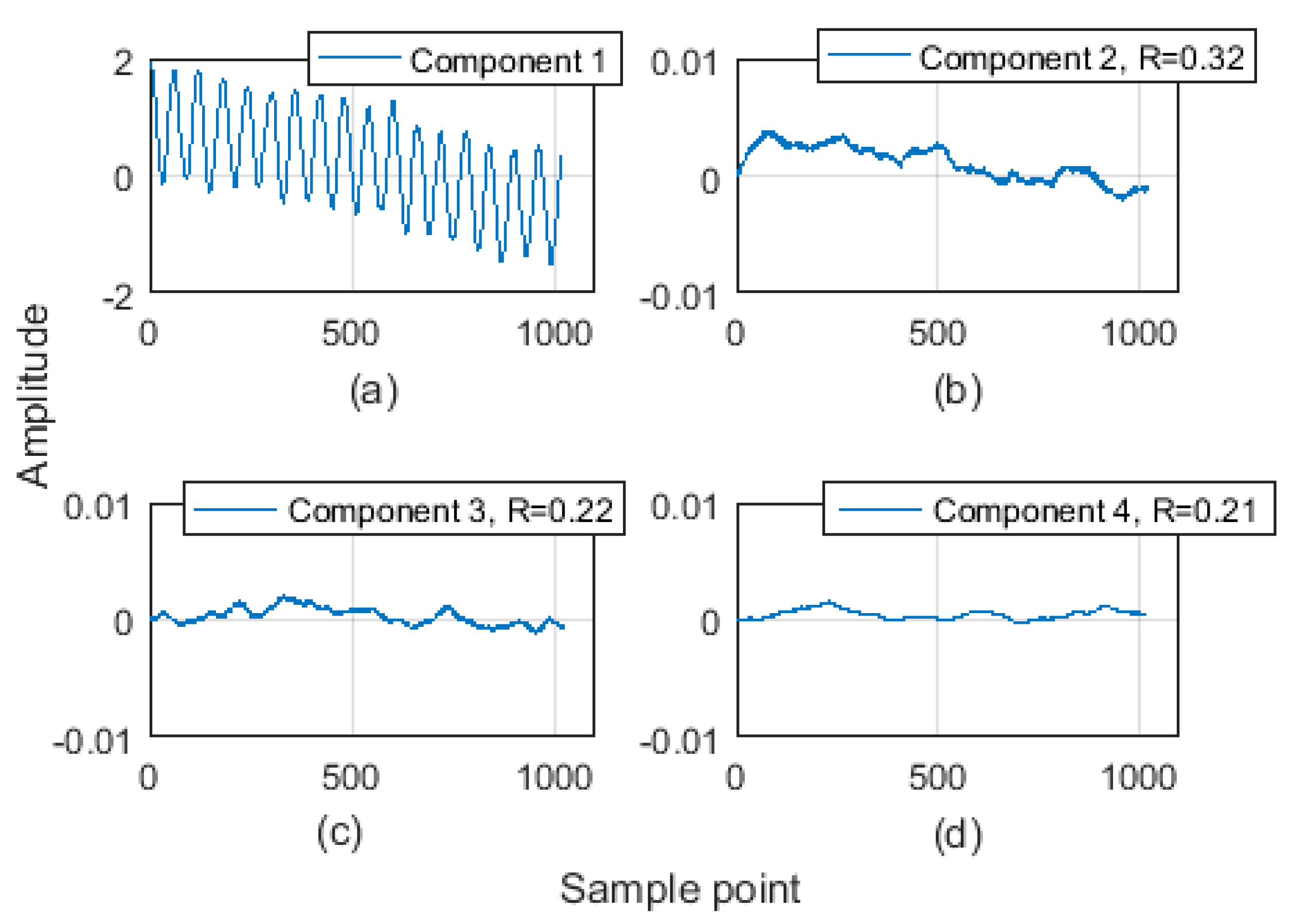
To present the superiority of the proposed SSA-AND de-noising algorithm, simulated noisy signal $Z\left(t\right)=\cos \left(2\pi t/2700\right)+\cos \left(2\pi t/60\right)+ \mathsf{\phi }\left(\mathrm{t}\right)$ is employed for verification, where $\mathsf{\phi }\left(\mathrm{t}\right)$ is random white noise. Firstly, the noisy signal $Z\left(t\right)$ is decomposed into components, as shown in Figure 1, we can see that the low frequency signal is extracted mainly in component 1 and high frequency noises are mainly in component 2, component 3, and component 4. Therefore, ANDs for each component should be designed separately. After decomposition, the next step is to calculate the CC of each component, as shown in

Table 1. The correlation coefficients of each component in Figure 1.

Parameters	Component 1	Component 2	Component 3	Component 4
Correlation Coefficient (CC)	0.78	0.30	0.21	0.20
Acceleration Factor (R)	0.82	0.32	0.22	0.21

, in which we can see that component 1 has the biggest CC. Then AND is applied on component1 to determine the first R of AND according to Step 3, then the other Rs can be calculated by Equation (10), as shown in Table 1.

Next step is the application of ANDs on components with determined Rs. It is of note that component 1 will be reserved directly without any processing, which can guarantee there is no signal delay or low frequency component. Figure 2 is the de-noising results of each component by using ANDs with determined Rs. We can see that: The details of component 1 are reserved totally; component 2 is filtered by AND with R = 0.32 which makes part of the details is reserved, and signal delay is occurred compared to Figure 1b; and component 3 to component 4 are filtered by AND with bigger Rs which make a set of smooth de-noising results are obtained, and it goes without saying that the signal delays are occurred.

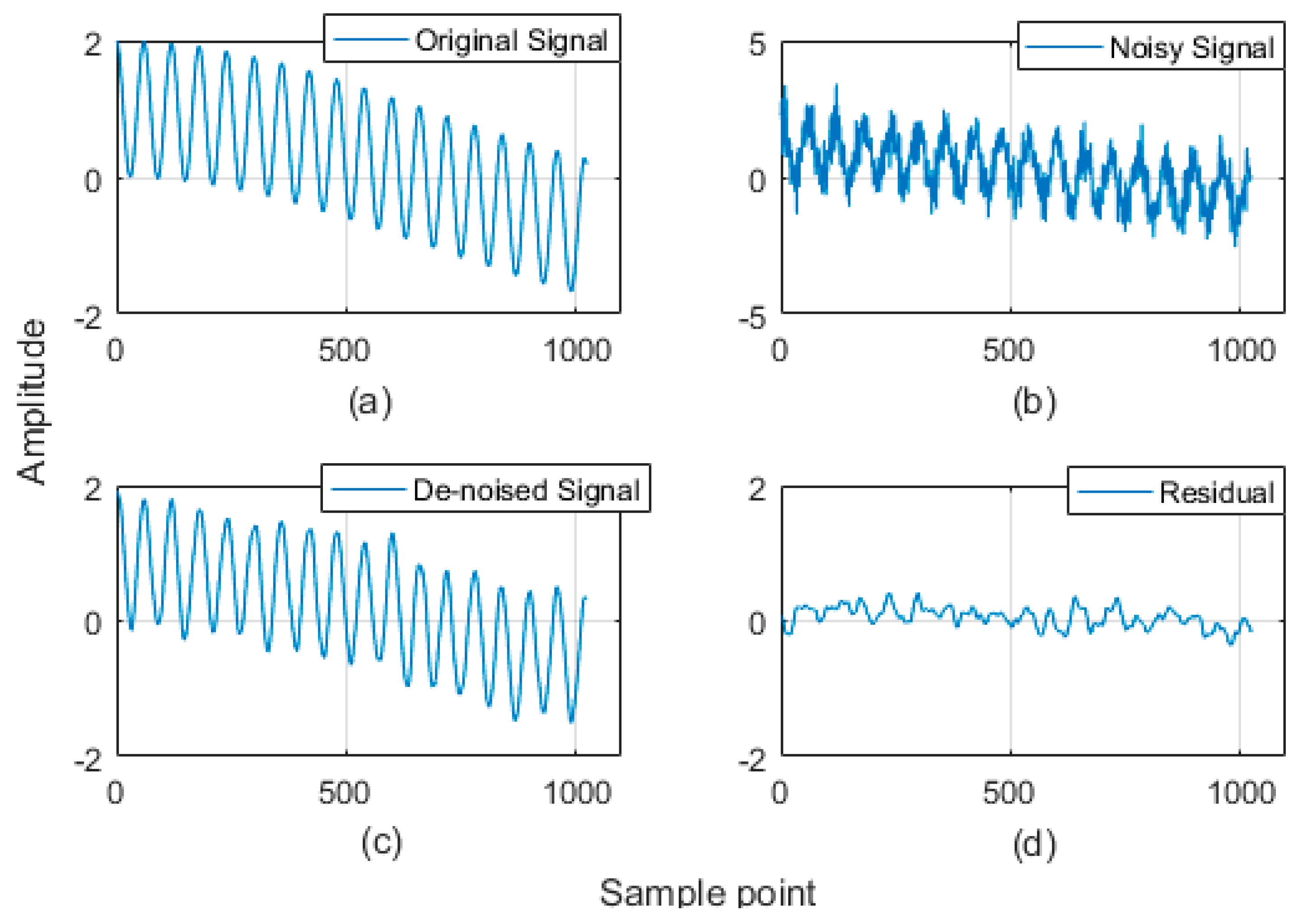
The last step is reconstruction. All the filtered components in Figure 2 are added together and then the reconstruction result is obtained, which is shown as Figure 3c. Comparison between Figure 3a–c show that the noise is reduced effectively; comparison between Figure 3a–c show that there is almost no signal delay occurred after de-noising by the proposed SSA-AND algorithm due to the low frequency component1 is reserved totally; from Figure 3d it can be seen that the residual still exists, which means the noise-attenuation ability or signal distortion problem of AND still need to be considered which would be our future work.

Furthermore, to verify the robustness of the proposed SSA-AND de-noising algorithm, we added the corresponding noise with different signal-to-noise power ratios (SNRs) for simulation. Additionally, some other advanced de-noising methods, such as Adaptive Robust Kalman Filter (ARKF), Detrended Fluctuation Analysis-VMD (DFA-VMD), empirical mode decomposition-forward linear prediction (EMD-FLP) and traditional AND are employed for comparison. In ARKF algorithm, the measurement noise covariance matrix is adapted using the weighted covariance of the innovation sequence which improves its robustness [13]. In combination of DFA and VMD, the number of band-limited intrinsic mode functions (BLIMF) decomposed by VMD is determined by DFA, aiming to avoid the impact of over-binning or under-binning on the VMD de-noising [24]. EMD-FLP algorithm is a hybrid de-noising algorithm, by using which noisy signal is decomposed into intrinsic mode functions (IMFs) first, and then each IMF is de-noised by forward linear prediction (FLP) [18]. The comparison results are shown in

Table 2. Comparison of the singular spectrum analysis-augmented nonlinear differentiator (SSA-AND) to other de-noising methods with different signal-to-noise power ratios (SNRs). EMD-FLP: empirical mode decomposition-forward linear prediction; DFA-VMD: detrended fluctuation analysis-variational mode decomposition; ARKF: adaptive robust Kalman filter.

SNR (dB)	−20	−16	−9	−3	0	3	6	9	11	13	16
EMD-FLP	−14.51	−10.23	−3.63	1.76	3.29	7.85	9.67	11.96	15.79	18.34	21.15
DFA-VMD	−16.55	−12.35	−5.59	0.38	6.54	6.48	12.77	12.47	16.73	18.90	22.56
ARKF	−12.71	−9.21	−0.41	4.69	7.12	10.30	13.49	15.68	19.59	21.30	24.87
SSA-AND	−10.3	−4.78	0.75	4.33	9.02	11.87	12.93	16.75	17.33	19.90	21.88

, and we can see that the SNR can be improved by using SSA-AND algorithm effectively from SNR’s range from + 20 dB to −20 dB, which also proves the excellent robustness of the proposed method.

4. Experimental and Verification

In this section, the output of FOG is employed for verifying the effectiveness of SSA-AND de-noising algorithm. Figure 4 is the experimental setup of FOG. The equipment is mainly including: Temperature control cabinet, a single axis FOG sensor, data acquisition system, computer, and (alternating current) AC-(direct current) DC converter. The diameter of the FOG is 11.5 cm, and the height is 2.5 cm.

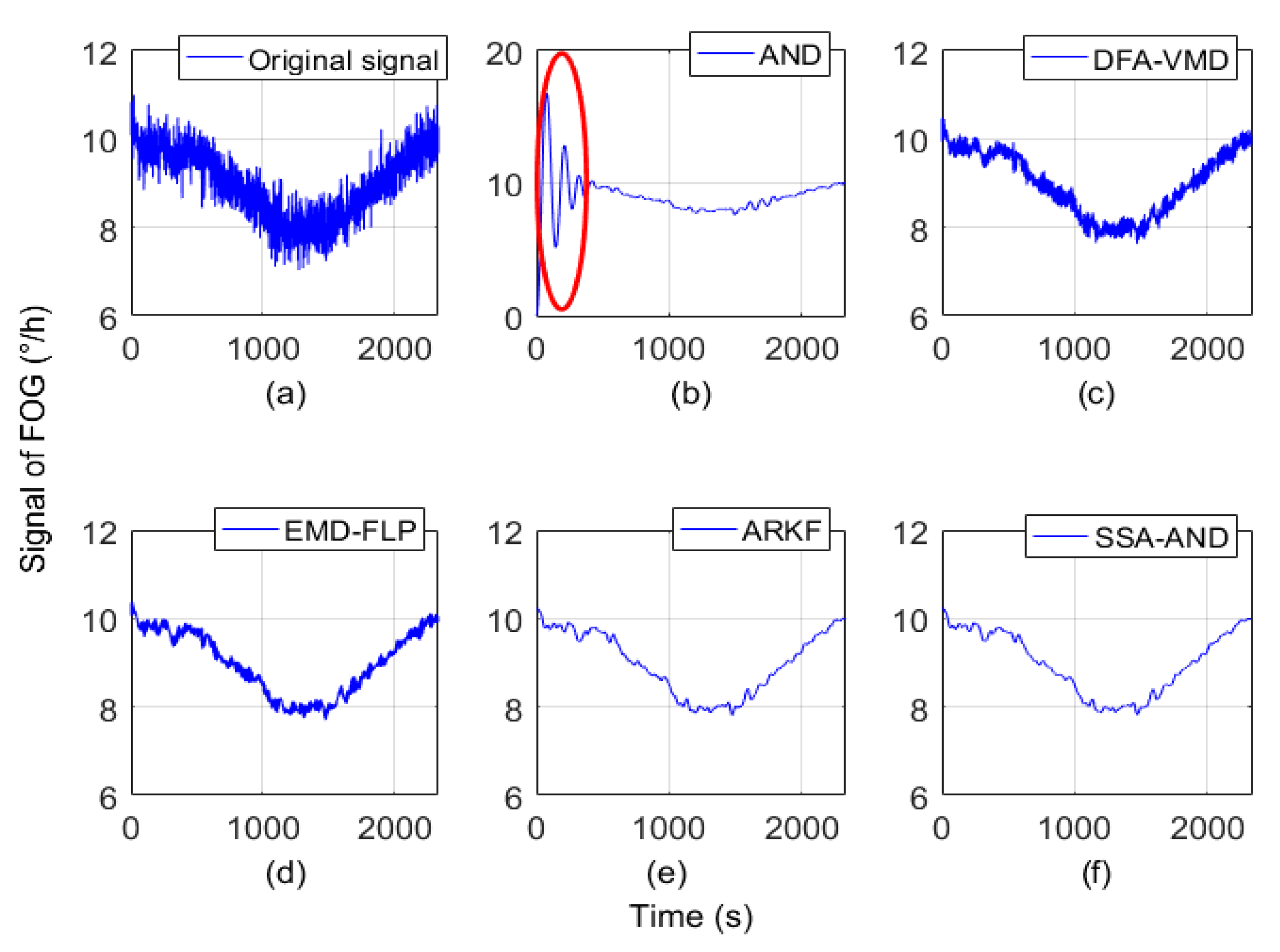
In this work, two set of data are collected from two different FOGs with temperature changing from +10 °C to −10 °C to +10 °C, where the temperature change rate is less than 1 °C /min. The two FOGs are the same type but different production batch. Figure 5a is the collected data from FOG1, and Figure 6a is FOG2. From the two figures we can see that, during the temperature variation, there is an obvious drift trend which is submerged in large noises. To extract the precise drift, it is necessary to eliminate the noises effectively. The de-noising procedure by using SSA-AND algorithm for FOG output signal is the same as Section 2. The comparison results are shown in Figure 5 and Figure 6.

From Figure 5 and Figure 6, all the de-noising methods can eliminate the noise of FOG output in some degree. Figure 5b and Figure 6b both show that when AND is used for de-noising alone, the signal delay phenomenon occurred, while there is almost no signal delay by using the proposed SSA-AND algorithm. From the step 3 of SSA-AND algorithm we know that after calculation of correlation coefficients, the strongest correlated component will remain entirely, which would ensure both no obvious signal delay after signal reconstruction and no damage of useful low frequency information. Compared to DFA-VMD algorithm, the de-noising result of SSA-AND algorithm seems better. According to the process of DFA-VMD algorithm, the function of DFA is defined to select the relevant modes to construct the de-noised signal, which means that the components with smaller DFAs would be abandoned, and the rest of components remained for reconstruction, therefore the noise in the remained components will be reserved. While in the process of SSA-AND, almost all the components would be processed by AND except the component with the biggest correlation coefficient, and the smaller correlated components would be suppressed strictly, therefore the de-noising performance of SSA-AND algorithm is better. The principle of EMD-FLP algorithm decomposes the signal into IMFs by EMD and then filter each IMF by FLP, which is similar as our proposed SSA-AND algorithm. However, there is no selection criterion for the parameters of FLP for each IMF which means that it is hard to select the best parameters just by experience, therefore the de-noising result of EMD-FLP algorithm is not optimal. Compared to AND, DFA-VMD, and EMD-FLP, a better de-noising result can be obtained by using ARKF. But the de-noising result of ARKF is still not as smooth as SSA-AND algorithm, that is because ARKF is de-noising the signal in time-domain directly, while the SSA-AND algorithm is decomposing the time domain signal into different components firstly and then each component is de-noised independently which makes the de-noising process more specific. Besides, compared to ARKF, it does not need to pre-design any model in the application of SSA-AND, which makes the structure of the proposed algorithm simpler.

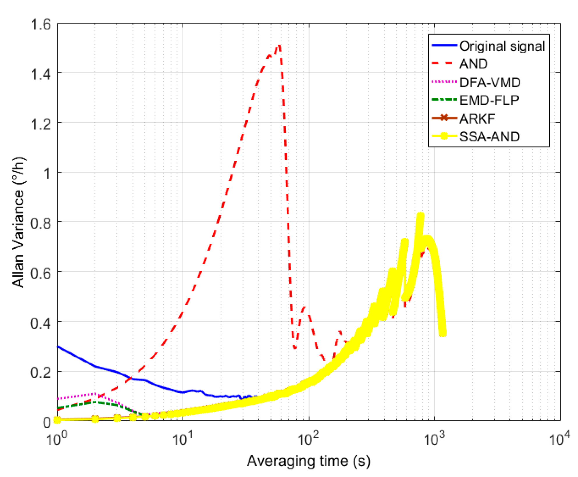
Moreover, Allan variance analysis is introduced to provide the quantitative comparison for de-noising results of different methods. Allan variance analysis has advantages in evaluating and identifying random noise coefficients. The random noise coefficients are Q (quantification noise, QN), N (angle random walk, ARW), B (bias instability, BI), K (rate random walk, RRW), and R (angular rate ramp, ARR), respectively. Among these parameters, ARW is the most widely used for representing the white noise, and QN stands for the noise induced by A/D and D/A conversion. Therefore, ARW and QN are the most important parameters for the determination of noise. Figure 7 and Figure 8 are the Allan standard deviation curves of de-noising results.

Table 3. Allan variance analysis results after de-noising of FOG1 and FOG2.

	Q($\mathit{\mu }$ rad)		N(°/h1/2)		B (°/h)		K(°/h3/2)		R(°/h2)
	FOG1	FOG2	FOG1	FOG2	FOG1	FOG2	FOG1	FOG2	FOG1	FOG2
Original	4.56	3.38	0.026	0.021	0.52	0.63	1.51	4.02	3.31	4.92
AND	5.50	4.08	0.027	0.019	1.29	1.04	4.87	2.74	6.73	3.85
DFA-VMD	1.82	3.14	0.0091	0.020	0.49	0.63	1.23	4.02	3.08	4.91
EMD-FLP	3.51	3.34	0.019	0.020	0.52	0.63	1.48	4.02	3.28	4.91
ARKF	2.08	2.88	0.010	0.015	0.51	0.62	1.39	4.01	3.21	4.91
SSA-AND	1.45	2.70	0.0083	0.013	0.48	0.62	1.23	4.01	3.07	4.91

shows the quantitative results. From Table 3 we can see that, after denoising, the ARW (N) and QN (Q) are reduced effectively. Take FOG1 as example, the ARW is reduced from 0.026 °/h^1/2 to 0.0083 °/h^1/2 by using the proposed SSA-AND algorithm, and the QN is reduced from 4.56 $\mu$ rad to 1.45 $\mu$ rad. Meanwhile, from Table 3 we can see that the SSA-AND algorithm performs better than other de-noising methods, which proves the superiority.

5. Conclusions

To minimize the random noise of FOG, an SSA-AND de-noising algorithm is proposed. Temperature experimental of FOG is carried out and the data are collected to verify the proposed SSA-AND algorithm. It can be concluded that the proposed SSA-AND algorithm has the best de-noising ability compared to other advanced de-noising algorithms, and the temperature drift of FOG can be extracted effectively without signal delay. The advantages of the proposed SSA-AND algorithm can be summarized as: (1) By combining SSA and AND together, the de-noising ability is enhanced effectively, and the signal delay caused by AND is eliminated; and (2) based on the correlation coefficient of each decomposed component, a parameter determination method for SSA-AND algorithm is proposed, which can be used as a reference for other similar hybrid de-noising methods based on multi-scale decomposition.

References

- Ying, D.Q.; Wang, Z.Y.; Ye, K.B.; Xie, T.; Mao, J.M.; Jin, Z.H. An open-loop RFOG based on 2nd/4th harmonic feedback technique to suppress phase modulation index’s drift. Opt. Commun. 2018, 426, 427–434. [Google Scholar] [CrossRef]
- Song, R.; Chen, X.Y.; Huang, H.Q. Nonstationary dynamic stochastic error analysis of fiber optic gyroscope based on optimized Allan variance. Sens. Actuators. A Phys. 2018, 276, 26–33. [Google Scholar] [CrossRef]
- Shen, C.; Song, R.; Li, J.; Zhang, X.M.; Tang, J.; Shi, Y.B.; Liu, J.; Cao, H.L. Temperature drift modeling of MEMS gyroscope based on genetic-Elman neural network. Mech. Syst. Signal Process. 2016, 72–73, 897–905. [Google Scholar]
- Ren, C.H.; Hu, X.M.; Qin, P.Y.; Li, L.L.; He, T. Signal filtering for small-diameter, dual-axis FOG inclinometer. Sens. Rev. 2018, 38, 353–359. [Google Scholar] [CrossRef]
- Jin, J.; Zhang, T.; Kong, L.H.; Ma, K. In-orbit performance evaluation of a spaceborne high precision fiber optic gyroscope. Sensors 2018, 18, 106. [Google Scholar] [CrossRef] [PubMed]
- Chen, X.Y.; Wang, W. Extracting and compensating for FOG vibration error based on improved empirical mode decomposition with masking signal. Appl. Opt. 2017, 56, 3848–3856. [Google Scholar] [CrossRef] [PubMed]
- Song, R.; Chen, X.Y. Analysis of fiber optic gyroscope vibration error based on improved local mean decomposition and kernel principal component analysis. Appl. Opt. 2017, 56, 2265–2272. [Google Scholar] [CrossRef] [PubMed]
- Yi, C.C.; Lv, Y.; Xiao, H.; Xiao, G.H.; You, G.H.; Dang, Z. Research on the blind source separation method based on regenerated phase-shifted sinusoid-assisted EMD and its application in diagnosing rolling-bearing faults. Appl. Sci. 2017, 7, 414. [Google Scholar] [CrossRef]
- Moreno, S.R.; Coelho, L.D. Wind speed forecasting approach based on singular spectrum analysis and adaptive neuro fuzzy inference system. Renew. Energy 2018, 126, 736–754. [Google Scholar] [CrossRef]
- Pal, C. Singular spectrum analysis, harmonic regression and EI-Nino effect on total ozone (1979-1993) over India and surrounding regions. J. Earth Sci. 2018, 127, 1–13. [Google Scholar] [CrossRef]
- Zhang, L.; Wang, Z.B.; Tan, C.; Si, L.; Liu, X.H.; Feng, S. A fruit fly-optimized Kalman filter algorithm for pushing distance estimation of a hydraulic powered roof support through tuning covariance. Appl. Sci. 2016, 6, 299. [Google Scholar] [CrossRef]
- Zhang, C.X.; Wang, L.; Gao, S.; Lin, T.; Li, X.M. Vibration noise modeling for measurement while drilling system based on FOGs. Sensors 2017, 17, 367. [Google Scholar] [CrossRef] [PubMed]
- Narasimhappa, M.; Sabat, S.L.; Peesapati, R.; Nayak, J. Fiber-optic gyroscope signal denoising using an adaptive robust Kalman filter. IEEE Sens. J. 2016, 16, 3711–3718. [Google Scholar] [CrossRef]
- Narasimhappa, M.; Nayak, J.; Terra, M.H.; Sabat, S.L. ARMA model based adaptive unsented fading Kalman filter for reducing drift of fiber optic gyroscope. Sens. Actuators A Phys. 2016, 251, 42–51. [Google Scholar] [CrossRef]
- Zhang, Y.; Shen, C.; Tang, T.; Liu, J. Hybrid algorithm based on MDF-CKF and RF for GPS/INS system during GPS outages (April 2018). IEEE Access 2018, 6, 35343–35354. [Google Scholar] [CrossRef]
- Shen, C.; Li, J.; Zhang, X.M.; Shi, Y.B.; Tang, J.; Cao, H.L.; Liu, J. A noise reduction method for dual-mass micro-electromechanical gyroscopes based on sample entropy empirical mode decomposition and time-frequency peak filtering. Sensors 2016, 16, 796. [Google Scholar] [CrossRef] [PubMed]
- Guo, X.T.; Sun, C.; Wang, P.; Huang, L. A hybrid method for MEMS gyroscope signal error compensation. Sens. Rev. 2018, 38, 517–525. [Google Scholar] [CrossRef]
- Shen, C.; Cao, H.L.; Li, J.; Tang, J.; Zhang, X.M.; Shi, Y.B.; Yang, W.; Liu, J. Hybrid de-noising approach for fiber optic gyroscopes combing improved empirical mode decomposition and forward linear prediction algorithms. Rev. Sci. Instrum. 2016, 87, 033305. [Google Scholar] [CrossRef] [PubMed]
- Castaneda, H.; Plestan, F.; Chriette, A.; de Leon-Morales, J. Continuous differentiator based on adaptive second-order sliding-mode control for a 3-DOF helicopter. IEEE Trans. Ind. Electron. 2016, 63, 5786–5793. [Google Scholar] [CrossRef]
- Dehkordi, N.M.; Sadati, N.; Hamzeh, M. A robust backstepping high-order sliding mode control strategy for grid-connected DG units with harmonic/interharmonic current compensation capability. IEEE Trans. Sustain. Energy 2017, 8, 561–572. [Google Scholar] [CrossRef]
- Lan, Q.X.; Qian, C.J.; Li, S.H. Finite-time disturbance observer design and attitude tracking control of a rigid spacecraft. J. Dyn. Syst. Meas. Control 2017, 139, 061010. [Google Scholar] [CrossRef]
- Shao, X.L.; Wang, H.L. Back-stepping robust linearization control for hypersonic reentry vehicle via novel tracking differentiator. J. Frankl. Inst. 2016, 353, 1957–1984. [Google Scholar] [CrossRef]
- Shao, X.L.; Liu, J.; Yang, W.; Tang, J.; Li, J. Augmented nonlinear differentiator design. Mech. Syst. Signal Process. 2017, 90, 268–284. [Google Scholar] [CrossRef]
- Liu, Y.Y.; Yang, G.L.; Li, M.; Yin, H.L. Variational mode decomposition denoising combined the detrended fluctuation analysis. Signal Process. 2016, 125, 349–364. [Google Scholar] [CrossRef]
Figure 1.
Decomposition results of (a) component 1 of decomposition results; (b) component 2; (c) component 3; (d) component 4.
Figure 2.
De-noising results of each component by using augmented nonlinear differentiator (AND) with determined Rs: (a) component 1 without de-noising; (b) component 2 denoising result with R = 0.32; (c) component 3 denoising result with R = 0.22; (d) component 2 denoising result with R = 0.21.
Figure 3.
Reconstruction results and comparisons: (a) original signal; (b) original signal added with noise; (c) de-noised signal by using SSA-AND; (d) residual.
Figure 4.
Experimental equipment arrangement of fiber optic gyroscope (FOG).
Figure 5.
Comparison results of different de-noising methods for the signal of FOG1: (a) original signal; (b) signal de-noised by AND with R = 0.5, the red circle shows the signal delay happens when using AND; (c) signal de-noised by DFA-VMD; (d) signal de-noised by EMD-FLP; (e) signal de-noised by ARKF; (f) signal de-noised by SSA-AND. AND: augmented nonlinear differentiator; DFA-VMD: detrended fluctuation analysis-variational mode decomposition; ARKF: adaptive robust Kalman filter; EMD-FLP: empirical mode decomposition-forward linear prediction; SSA-AND: singular spectrum analysis-augmented nonlinear differentiator.
Figure 6.
Comparison results of different de-noising methods for the signal of FOG2: (a) original signal; (b) signal de-noised by AND, where R = 0.5; (c) signal de-noised by DFA-VMD; (d) signal de-noised by EMD-FLP; (e) signal de-noised by ARKF; (f) signal de-noised by SSA-AND.
Figure 7.
Allan variances analysis for FOG1.
Figure 8.
Allan variances analysis for FOG2.