Article

A New Hybrid Approach for Wind Speed Forecasting Applying Support Vector Machine with Ensemble Empirical Mode Decomposition and Cuckoo Search Algorithm

1
Faculty of Professions, University of Adelaide, Adelaide 5000, Australia
2
School of Statistics, Dongbei University of Finance and Economics, Dalian 116025, China
*
Author to whom correspondence should be addressed.
Appl. Sci. 2018, 8(10), 1754; https://doi.org/10.3390/app8101754
Submission received: 12 July 2018 / Revised: 17 September 2018 / Accepted: 20 September 2018 / Published: 28 September 2018
(This article belongs to the Special Issue Sustainable Energy Systems Planning, Integration and Management)

Abstract

:

Featured Application

Wind speed forecasting.

Abstract

Wind speed forecasting plays a crucial role in improving the efficiency of wind farms, and increases the competitive advantage of wind power in the global electricity market. Many forecasting models have been proposed, aiming to enhance the forecast performance. However, some traditional models used in our experiment have the drawback of ignoring the importance of data preprocessing and the necessity of parameter optimization, which often results in poor forecasting performance. Therefore, in order to achieve a more satisfying performance in forecasting wind speed data, a new short-term wind speed forecasting method which consists of Ensemble Empirical Mode Decomposition (EEMD) for data preprocessing, and the Support Vector Machine (SVM)—whose key parameters are optimized by the Cuckoo Search Algorithm (CSO)—is developed in this paper. This method avoids the shortcomings of some traditional models and effectively enhances the forecasting ability. To test the prediction ability of the proposed model, 10 min wind speed data from wind farms in Shandong Province, China, are used for conducting experiments. The experimental results indicate that the proposed model cannot only improve the forecasting accuracy, but can also be an effective tool in assisting the management of wind power plants.

1. Introduction

1.1. Background and Motivation

In recent years, a demand for clean and renewable energy resources has increased significantly because of the air pollution caused by traditional fossil fuels. Wind power, which is one of the most promising renewable resources, proved to be an ideal alternative. Currently, wind energy has been successfully employed in many countries, representing approximately 10% of energy consumption in Europe and more than 15% in countries like America and Spain [1]. However, wind speed, which is one of the most essential factors in wind power generation, is difficult to forecast due to many natural factors such as pressure, temperature, and the rotation of the planet.
Therefore, in the development of wind energy, wind speed forecasting is rather important. The accuracy of the forecasting result can influence the wind rotating equipment, operation cost, and the limitations of wind power penetration. With a precise prediction of wind speed, the dispatching department is able to make adjustments to the program efficiently, so that the influence of wind energy itself on the power station and the adverse effect of the wind farm on the power system can be minimized, making wind power more competitive in the global electricity market.

1.2. Existing Models

Currently, developing an accurate and effective wind speed forecasting model is a priority in many countries. These models can be divided into four categories based on the specific time horizon: Very short-term, short-term, medium-term, and long-term forecasting [2]. Very short-term and short-term forecasting can provide aids and references when making economic load dispatch plans, while medium and long-term forecasting are employed for the maintenance of the grid, wind farm planning, and providing information for site selection [3,4]. Using computational methods, these forecasting methods can be further categorized into four different types: Physical, statistical, intelligent, and hybrid methods. Physical methods are usually based on numerical weather prediction (NWP), which simulates the physical characteristics of the atmosphere through applying physical rules and geographical conditions, though there are still many difficulties in employing this model for wind speed forecasting directly—for example, the forecasting accuracy, resolutions of space and time, and the importance of the physical procedures. Statistical methods are used for wind speed forecasting through setting mathematical models, which are similar to the direct random time-series models [5]. As one of the most widely employed statistical methods, the Autoregressive Integrated Moving Average (ARIMA) model is adopted to predict wind speed. Moreover, an Autoregressive Fractional Integrated Moving Average (ARFIMA) model is used in wind speed prediction because of its superior ability to select valid information from the past time series more effectively, compared with the traditional ARIMA model. In recent years, intelligent approaches such as artificial neural networks (ANN) and back propagation neural networks (BP), with the aim of reducing errors by employing past time series, are being applied to forecast future wind speed because of the rising popularity of artificial intelligence [6,7,8,9,10,11,12].
Due to the complexity of the raw wind speed series, forecasting the traits in the time series accurately is very difficult to achieve with individual models. Therefore, hybrid models which adopt multiple approaches to increase the prediction ability of the raw time series, or which assemble multiple forecasting methods to obtain the traits of the raw data to forecast wind speed, have been proposed in many studies. Guo et al. combined the Seasonal Autoregressive Intergrated Moving Average model (SARIMA) and the Least Square Support Vector Machine model (LSSVM) to obtain a more accurate forecasting model [13]. This new approach can effectively catch the seasonal and nonlinear features in the input data. Similarly, Guo et al. used a back-propagation neural network, and relied on the theory of using a seasonal exponential adjustment to reduce seasonal influence from the raw data, to create a new hybrid approach [14]. Experimental results showed that this new model is able to effectively increase the forecasting precision, as compared to the results of an independent back propagation neural network (BPNN) with no adjustment of the seasonal exponent. From the studies of Pourmousavi et al., a new and very short-term wind speed hybrid model was proposed and proven to significantly increase the prediction range [15,16]. Liu et al. combined Empirical Model Decomposition to create a new hybrid Empirical Mode Decomposition-Artificial Neural Network (EMD-ANN) model. The proposed approach was effective in capturing jumping samples in raw data with high noise [17]. Mohammadi et al. proposed a Stackelberg game technique to improve the efficiency of electric grid [18]. Kianoosh et al. introduced a new multi-time-scale approach modeled by historical time-series for electric data forecasting [19]. Haque et al. put forward the idea of combining multiple soft computing models with a data preprocessing technique to perform short-term wind speed forecasting [20]. Li and Shi conducted an experiment to make a comprehensive comparison among three ANN using one h ahead of forecasting; namely, ADLINE (adaptive linear element), RBFNN (radial basis function neural network), and BPNN (back-propagation neural network) [21]. Moreover, to reduce the influence of data diversity, Ortiz-García et al. introduced several novel SVM structures, which achieved a better performance than a similar multilayer perception [22].

1.3. Introduction of the Proposed Model

However, these individual models mentioned above have certain drawbacks. The disadvantages are summarized as followed: (1) They usually require a huge amount of wind speed data in order to build a model for a precise prediction, because of the inner irregularity and instability within the raw data. If the raw data suddenly changes due to environmental factors, the error of the forecasting result can be relatively high [23]; (2) Some models only try to match the fitness of the model closer to the original data. As a result, when processing the wind speed data with high noise and irregularity, it is difficult to fit the individual model to it by using only traditional physical or statistical methods, causing poor forecasting accuracy and low efficiency; (3) Individual forecasting methods ignore the importance of data preprocessing and the necessity of model parameter optimization. Because of this, the accuracy of the result is not satisfying; (4) While some new models take advantage of artificial intelligence to enhance their forecasting ability, they still have the problem of over-fitting and a low convergence rate [24].
Therefore, in order to solve the problems mentioned above, a new hybrid model for more precise wind speed forecasting and better evaluation, achieved by adapting the Ensemble Empirical Mode Decomposition (EEMD), the Cuckoo Search Optimization (CSO) algorithm, and the Support Vector Machine (SVM) model, is introduced in this paper.
The main contributions and innovations of this paper compared to other studies in the field of wind speed forecasting are summed up as follows:
  • The newly proposed approach in this paper takes advantage of the data preprocessing method and the algorithm of parameter optimization to enhance the performance of the SVM model. In this paper, the raw time series is first decomposed into several sub-signals, among which signals with high frequency ones are removed and the rest are restructured to obtain a stationary time series, with which the intrinsic characteristics of the wind speed data can be better captured and analyzed so that the forecasting accuracy can be greatly improved.
  • This paper employs the Cuckoo Search algorithm to optimize the parameters of the SVM before training. The CS algorithm, which has the advantage of a powerful capability in terms of global optimization, requires few parameters and has strong multi-objective problem solving ability, and therefore can significantly improve the accuracy of the forecasting. The Support Vector Machine can overcome the difficulties of traditional models, such as the curse of dimensionality, falling into local optima easily, and over-learning.
  • To verify the forecasting ability of the proposed approach, conventional models like BPNN, RBFNN, and ARIMA are used for comparison. A more comprehensive evaluation is conducted, including multi-step forecasting experiments and performance evaluation metrics such as six indexes and a DM(Diebold-Mariano) test, to assess and analyze the performance of the newly developed method.
The model used the raw data from wind turbines in a large wind farm. The result of this paper shows that the newly developed approach effectively improves the forecasting accuracy and can be successfully applied in wind grids to provide statistical support for making operation plans and managing the power station.

1.4. Structure of the Paper

This paper is organized as follows. Section 2 concisely introduces the required techniques. Forecasting performance evaluation criterion and numerical experimentation are introduced in Section 3 and Section 4. In Section 5 and Section 6, the results and the superiority of the proposed approach are discussed by using comparisons with other conventional methods. Finally, Section 7 concludes this paper and introduces the direction for future studies.

2. Materials and Methods

In this section, main theories about the proposed model will be introduced first. Then, the proposed hybrid model is introduced. DM tests and forecasting effectiveness are also introduced.

2.1. Empirical Mode Decomposition (EMD)

EMD, which has been proved to be an effective data preprocessing method, is usually applied to reduce the noise of a time series, which is non-stationary [25]. The main theory of EMD is that by local characteristic timescale filtering, the original series is decomposed into oscillatory modes (IMFs). The IMFs follow the rules as shown below: (1) The extremes and the zeros must have the same quantity or the difference of quantity must be within one in the whole time series; (2) The upper and lower bounds’ mean must be equal to zero. Let the raw data be s ( t ) ( t = 1 , 2 , , l ) . The main procedures of EMD are listed below:
(a)
Set all local maxima and minima of time series.
(b)
Connect all local extreme to produce the upper bound e u p ( t ) and the lower bound e l o w ( t ) by applying a cubic spline.
(c)
Compute the mean value from the upper and lower bounds m ( t ) = [ e u p ( t ) + e l o w ( t ) ] / 2 .
(d)
Compute the difference value between the raw data and the mean value h ( t ) = s ( t ) m ( t ) .
(e)
Inspect if h ( t ) fits characteristics of IMF. If yes, h ( t ) is defined as the ith IMF and the residual r ( t ) = s ( t ) h ( t ) will replace s ( t ) . If no, s ( t ) will be replaced by h ( t ) .
(f)
Repeat the above-mentioned procedures. Stop when the value of the two successive siftings’ standard deviation is lower than the threshold set earlier.
By utilizing mentioned procedures, a group of IMFs is settled from the raw data, which is arranged based on the frequency from high to low.
Definition 1.
The raw data, which is used for decomposition and consists of n IMFs and one residual is obtained as:
s ( t ) = i = 1 n c i ( t ) + r n ( t )
where n is the number of IMFs, r n ( t ) is the residuals representing a trend in s ( t ) ( t = 1 , 2 , , l ) , and c i ( t ) ( i = 1 , 2 , , n ) represents the IMFs. When describing the local characters of a raw time series, each IMF is independent.

2.2. Ensemble Empirical Mode Decomposition (EEMD)

EEMD, which can successfully overcome the shortcomings of EMD, is first introduced by Wu and Huang [26]. The main theory of EEMD is that by using the features of the noise, the problem of mode mixing can be effectively solved. The original time series are combined with true signals and noise. Thus, to extract the true signals in the raw data, a white noise is added to the original data. Procedures of EEMD can be described as follows.
  • Step (a). Add a white noise to the raw time series.
  • Step (b). Based on the method of EMD, decompose the time series with the added white noise to nIMFs.
  • Step (c). Repeat the mentioned two steps, but add the white noise at different scales each time.
  • Step (d). Calculate the means of each IMF of decomposition to constitute the final IMFs.
Through the mentioned process, the whole series of white noise, which are added into the raw data, can provide a unified reference range to assist the process of noise reduction. As a result, the true IMFs can be obtained from the original data.
Definition 2.
The relationship among the ensemble number, the error tolerance, and the added noise level is described based on the research of Wu and Huang:
N ε = ε 2 ε n 2
where ε represents the amplitude of the added noise, ε n is the error’s standard deviation, and N ε is value of ensemble members. Generally, it is suggested that an amplitude fixed at 0.2 will result in an accurate result [26]. In this study, the value of ensemble members are set to 100 and the optimal standard deviation of white noise series are settled from 0.1 to 0.2.

2.3. Cuckoo Search Optimization (CSO) Algorithm

The CSO, which was recently introduced by Yang et al., is a meta-heuristic search algorithm [27]. The main principle of the algorithm is originated from the application of cuckoo birds’ obligating brood parasitic behavior and the behavior of Lévy flight. Generally, by the switching/discovery probability (pa), Cuckoo Search algorithm is able to perform more powerful capability of optimization [28]. In order to successfully adopt the CS algorithm, three basic assumptions are illustrated as follows:
  • The egg which is generated by each cuckoo bird represents a solution in a time period, and it is dumped randomly in the nest.
  • The nests which contain better eggs (better solution) are described as the best nests and they will be passed to the next generation.
  • The available host nests’ number is restricted to n, and each host bird is able to recognize the cuckoo bird’s egg with a probability P a [ 0 , 1 ] . As a result, the host bird has two possible choices, which are either throwing away the egg or giving up the whole nest and finding a new location to build a new nest.
Definition 3.
Based on the Lévy flight behavior of the cuckoo bird’s nest-seeking nature, set the current solution as x i t for i th cuckoo, then new solution x i t + 1 is generated as follows:
x i t + 1 = x i t + α L ( λ ) , i = 1 , 2 , 3 n L ( λ ) = t λ , ( 1 < λ 3 )
where α > 0 is the size of each step which relates to the optimization. ⊕ is the entry wise multiplications. L ( λ ) stands for a Lévy distribution which has an infinite mean and variance. Lévy flight essentially provides a random walk while the random step length is drawn from L ( λ ) , which can produce a random walk process. Around the best solution, the local search process can be faster because of the new solution generated by Lévy walk [29]. The flowchart of CSO is shown in Figure 1.

2.4. Support Vector Machine (SVM)

The Support vector machine, which is introduced by Vapnik, is one of the newest algorithms [30]. Different from the conventional models, SVM follows the rule of statistical machine learning process and structural risk minimization to obtain the minimal upper bound generalization error, which is the biggest advantage of SVM compared with other models. Due to this, SVM has a great popularity and a wide use in the area of pattern recognition, classification, and regression analysis and forecasting [31,32].
Definition 4.
Suppose a set of data { x i d i } i n , the n-dimensional input vector is represented as x i , and the output is expressed as d i . The estimating function of SVM can be represented as:
f ( x ) = w · ϕ ( x ) + b
where ϕ ( x ) is a nonlinear mapping while w, b is the weight vector and scalar, separately, and they are estimated through the equation:
R S V M s ( C ) = 1 2 w 2 + C 1 n i = 1 n L ( x i , d i )
where C represents the penalty factor of the error. The L ( x i , d i ) is the loss function C n 2 i = 1 n L ( x i , d i ) represents the empirical error.
Definition 5.
Setting the upper and lower excess deviation ξ i and ξ i * as the positive slack variables, the optimization problem is obtained as the follows:
M i n i m i z e R S V M s ( w , ξ ( ) ) = 1 2 w 2 + C 1 n i = 1 n ( ξ i + ξ i )
S u b j e c t   t o { d i w ϕ ( x i ) b i ε + ξ i w ϕ ( x i ) + b i d i ε + ξ i ξ i , ξ i 0 , i = 1 , , l
where w 2 / 2 represents the regularization term. ε stands for the loss factor, and its value is related to the approximate accuracy of the input sample. l represents the quantity of elements in the sample data series.
Equation (4) can be explained through the Lagrange function, which is described as follows:
f ( x ) = i = 1 n ( α i α i ) K ( x , x i ) + b
where α i and α i * are the multipliers of Lagrange function. K ( x , x i ) represents the kernel function and K ( x i , x j ) = ϕ ( x i ) ϕ ( x j ) , which is the dot product of the two inner vectors x i , x j in ϕ ( x i ) and ϕ ( x j ) .
Gaussian function, which is known for its features of simplicity, efficiency, and reliable computing ability, has proved to be one of the most effective core functions [30]. SVM model, which employs it as the core function, can effectively obtain the complex features of nonlinearity of the original data and result sample by matching input data into a higher-dimensional feature space.
Definition 6.
Gaussian function, which is employed as core function of SVM model, is described as follows:
K ( x i , x j ) = exp ( γ x i x j 2 )
where the γ stands for the parameter of the kernel function. xi, xj are vector quantities in the input space.
In this paper, parameters (γ, C), which are considered as the two most valuable figures that influence the performance of wind speed prediction. The CSO is used to optimize them.

2.5. Introduction of the EEMD-CSO-SVM Model

Based on the above-mentioned methods, the EEMD-CSO-SVM model is proposed for wind speed forecasting. Taking one of the datasets as an example, the main procedures of the proposed model is shown in Figure 2. Firstly, the EEMD noise reduction technique is applied to the raw wind speed data in order to obtain a stationary time series. In this paper, the raw data is decomposed into 10 IMFs, among which the first IMF is considered as noise and removed. The rest are recombined for the forecasting. Then, each set of data from the four wind turbines are used to perform three-step forecasting to testify the validity of the proposed model. The de-noised wind speed data is applied to train the SVM model whose key parameters (γ, C) are optimized by the Cuckoo Search algorithm. The results of forecasting are recorded for further analysis.

2.6. DM Test and Forecasting Effectiveness

The DM test, which focuses on the difference in the forecasting precision between the proposed hybrid model and other traditional methods, is described as follows:
H 0 : E ( d n ) = 0 , n H 1 : E ( d n ) 0 , n
The value of the DM test is described as follows:
DM = h = 1 k ( L ( ε t + h ( i ) ) L ( ε t + h ( j ) ) ) / k S 2 / k s 2
where ε t + h is the forecasting error.
S 2 represents the estimation value for the variance of d h = L ( ε t + h ( i ) ) L ( ε t + h ( j ) ) . L is the loss function, which represents the accuracy of the forecasting.
Among the loss functions, absolute deviation error loss and square error loss are widely applied. They are described as follows:
Absolute deviation error loss:
L ( ε t + h ( i ) ) = | ε t + h ( i ) |
Square error loss:
L ( ε t + h ( i ) ) = ( ε t + h ( i ) ) 2
If no significant differences are found between the performances of the included methods, the null hypothesis will be rejected.
The null hypothesis is described as follows:
| DM | > z α / 2
where z α / 2 represents the critical value of the standard value distribution when the value of significance is α.
Forecasting effectiveness, which evaluates the performance of the proposed model using the sum of the squared errors and the mean squared deviation of the forecasting results is also applied. The forecasting effectiveness is described as follows [33].
The kth order forecasting effectiveness unit is described as:
m k = n = 1 N Q n A n k n = 1 N Q n = 1
where Qn stands for the discrete probability distribution when the time is n. An represents the forecasting accuracy.
The k-order forecasting effectiveness is presented as:
H ( m 1 , m 2 , , m k )
The first order forecasting effectiveness is defined as H ( m 1 ) = m 1 while the second-order forecasting effectiveness is the difference between the standard deviation and expectation, which is shown as:
H ( m 1 , m 2 ) = m 1 ( 1 m 2 ( m 1 ) 2 )

3. Performance Evaluation Criterion

In this study, to test the accuracy of the proposed approach, six evaluation indexes including MAE, MAPE, RMSE, WI, ENS, and ELM are applied for evaluating forecasting accuracy. These indexes are shown as follows in Table 1:
Respectively, where N is the total output samples; yi represents the actual series; and ypi stands for the prediction results. For WI, ENS, and ELM, when the values of them are closer to 1, the model achieves a higher performance.

4. Numerical Experimentation

The Windows 7 Professional operating system was used to perform the experiments. The specific version of software, which was used to conduct the proposed model, is Matlab2016a. The details of the hardware are: Intel Core i5-3230M2.60 GHz CPU, and 4 GB RAM.

4.1. Introduction of Datasets

Penglai is located in the east coast of Shandong in China. It has a 3100 km coastline. Thus, although the whole region is not large, it is famous for its abundant wind power due to this unique geographical feature. The approximate wind power capacity of the region is 67 million KW. In this paper, datasets 1, 2, 3, and 4 were chosen from a wind farm in Penglai, with the latitude from 120°43′ N to 120°47′ N and longitude from 37°50′ E to 37°37′ E. These datasets are located in mountain and hilly areas whose altitude is from 100 m to 240 m. The features of the wind power generator are provided as follows: Rated power: 1500 KW. Height of measurement: 70 m. Sampling time period: 10 min. Scanning frequency: 144 times per day. All four datasets were included in the experiment, to help analyze the differences in the results. Multistep forecasting was also conducted in this paper.
Each group is divided into a training group and a testing group. The size ratio of the training and testing group is set to 9:1. The training sample included a total of 1350 10-min wind speed series, and the testing sample contains 150 wind speed data points. The ratio of input and output data is set to 4:1. Figure 3 shows the structure of each dataset.

4.2. Forecasting Model Parameter Setting

Wind speed series from four datasets are chosen to test the forecasting accuracy of the proposed hybrid model. The results of the proposed model are also used to compare with other conventional methods; namely, BP neural networks, the ARIMA model, and the RBF model. This paper followed the standard of energy industry NB/T31046-2013 and the rules for measuring wind sources, which were published and made by the National Energy Administration in 2013.
(1)
For BPNN, the newff function of the neural network toolbox is employed to build the network. The dimensions of the input, hidden, and output layers are 4, 5, and 1, respectively. The learning rate is set to 0.1, the maximum number of iterations is set to 100, and the training precision is set to 0.00004.
(2)
For ARIMA, the forecasting results are influenced by the moving average and the order of auto-regressive. The observed value’s fitting effect is measured by the AIC criterion, and the AIC also calculates the most suitable number for the parameters. When the AIC reaches the lowest value, the ARIMA method can achieve the best order.
(3)
For RBFNN, similar with BPNN, the newrb function of the neural network toolbox is employed to build the forecasting network. The same parameters as the BPNN are used in the RBFNN.

4.3. Experimental Results for Datasets

The original time series are first preprocessed through the EEMD. Figure 3 presents the preprocessed data obtained by the EEMD method for the four wind turbines. As indicated in Figure 3, for the #2, #3, and #4 wind turbines, 10 IMF sequences are obtained from the original training data of the time series. According to the principles of denoising, eliminating the high-frequency sequence from the IMF sequences can assist in obtaining a cleaner data sequence; that is, a data sequence with lower noise. For this paper, the first IMF sequence obtained by the EEMD method is eliminated from the original data sequence due to its high frequency, so that a stationary time series can be obtained to improve the accuracy of the prediction. Taking wind turbine #2’s data as an example, the visualization of the de-noise preprocessing of the EEMD method is shown in Figure 4. The final result after the de-noise processing with the EEMD method is also presented in Figure 4. The preprocessing results of all four wind turbines are shown in Figure 3.
For the experiment, the proposed method is trained using the selected data from four datasets. Multistep forecasting is applied in the experiment, which performs the prediction through removing the old input data for each circulation. By applying the previous output values rather than the actual series, the multistep ahead method predicts the next wind speed value through this circulation [34]. The one-step forecasting result is calculated based on the observed values from x1 to xn, where n is the number of output value. Two-step forecasting result is calculated based on the observed value from x2 to xn and the one-step result. Additionally, three-step forecasting result is obtained based on the observed value from x3 to xn and the previous two-steps results. The validity of the proposed hybrid model was analyzed based on the results of multistep ahead forecasting. Table 2, Table 3, Table 4 and Table 5 show the forecasting results of different models in four wind turbines, respectively. The results of multistep ahead forecasting are shown Table 6.
The performance of hybrid and traditional methods in one-step forecasting are compared. To testify the effectiveness of the CSO, Particle swarm optimization (PSO) is used for comparison. PSO, which is similar with CSO, optimizes the parameters based on the velocity of particle and the method of position updating. The MAPE values of the proposed hybrid are 4.79%, 3.07%, 2.69%, and 3.91% in four wind turbines, respectively. The values of Willmott’s Index reach 0.9838, 0.9929, 0.9918, and 0.9839, respectively. The other values of forecasting error indexes also indicate that the hybrid approach performs better than traditional methods. The results are shown in Table 2 and Table 3.
In the results of dataset 2, the MAPE values of the proposed model are 3.07%, 6.53%, and 10.70% in three-steps forecasting, separately, which shows that one step forecasting performs better. Multistep forecasting, which is based on the theory of removing old input data and adding new output data from the previous step, cannot achieve the same performance accuracy as single step forecasting.
Remark 1.
The hybrid approach includes more parameters so that better performance can be achieved. As for the multistep forecasting, its process is complex and leads to high error because less historical data is employed and the forecasted result of each step will be included as input in the next circulation. Therefore, with more steps of forecasting being conducted, more errors will appear, leading to poor performance.

5. Analysis of the Forecasting Results

This section analyzes the experimental results of the hybrid approach, and the effectiveness of the proposed method is verified. First, based on the results of single step forecasting, the hybrid approach is compared with some existing conventional models. Then, the results of multi-step forecasting are used for further analysis.

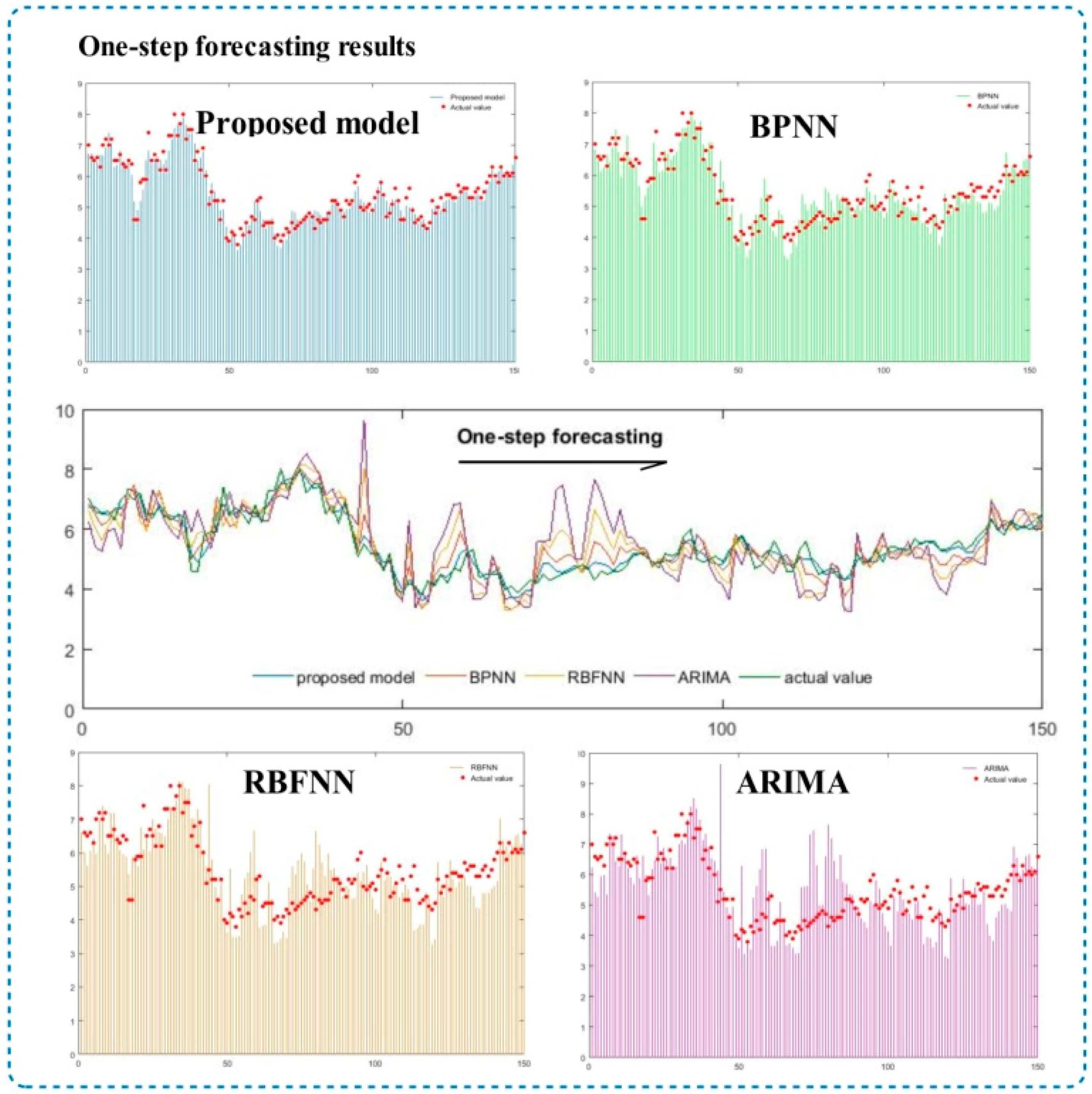
5.1. Single-Step Forecasting

This is divided into two parts to verify the effectiveness of the hybrid approach. First, the hybrid method is tested by comparing it with conventional methods. Then, the results of four different datasets are analyzed.

5.1.1. Analysis of the Proposed Method and Conventional Models

The forecasting results of the proposed model and conventional models are shown in Table 4 and Table 5. The original time series and preprocessed data obtained by the EEMD technique is shown in Figure 3. By comparing the results illustrated above, the following conclusions are made:
The fluctuation and instability of the original time series are clearly shown in Figure 3. Additionally, in Figure 3, the reconstructed wind speed data in which the signals with high frequency have been removed obviously shows reduced noise of the raw data. By comparing the forecasting results of the new preprocessed data with the original data from Table 2 and Table 3, the model achieves a high performance when using the de-noised wind speed data. The MAPE values of the CSOSVM model decrease by 5.88%, 5.56%, 2.39%, and 7.36%, respectively. Using the PSOSVM model for comparison, the MAPE values also decrease by 6.55%, 6.88%, 5.34%, and 5.71% in four datasets, respectively. Therefore, the EEMD technique has good validity.
The proposed hybrid approach achieves better performance than the conventional methods in wind speed prediction. From Table 4, the MAPE value of BPNN, RBFNN, ARIMA, and the proposed model in wind turbine 1 are 8.68%, 10.32%, 8.41%, and 4.79%, respectively. In the other three datasets the proposed method also achieves higher performance than other conventional methods. The values of the evaluation metrics shown in Table 4 and Table 5 all suggest that the hybrid model achieves higher accuracy. The new hybrid approach can be regarded as more effective than traditional methods.
Remark 2.
The data preprocessing technique is a reliable method to reduce the fluctuation in the raw data, and the EEMD proves to be an effective method to achieve this purpose. Therefore, the proposed hybrid approach outperforms the conventional methods in forecasting.

5.1.2. Analysis of the Four Different Wind Turbines

This paper employs four wind turbines to conduct the forecasting experiment of the wind speed. The original time series of the four datasets are presented in Figure 3. The results from the four different datasets using different approaches are shown in Table 2, Table 3, Table 4 and Table 5.
From Figure 3, the general trend of the four time series is approximately the same, though there are still differences in some time points. The main reason for this difference is that in a general location, the wind speed is nearly the same. However, when narrowing down to a specific wind farm unit, the location and size of the wind farm varies, resulting in different wind speed data from one dataset to another.
When analyzing from the specific forecasting results, according to the data presented in Table 4 for instance, the MAPE values of the proposed model from the four wind turbines are 4.79%, 3.07%, 2.69%, and 3.91%. For the forecasting accuracy, dataset 3 achieves the highest performance.
Remark 3.
Because of the uncertainty of the magnitude and direction of the wind in different locations, the forecasting results of four different datasets vary. The wind speed also experiences enormous fluctuations in different time periods. As a result, the prediction precision also varies due to different locations and time periods.

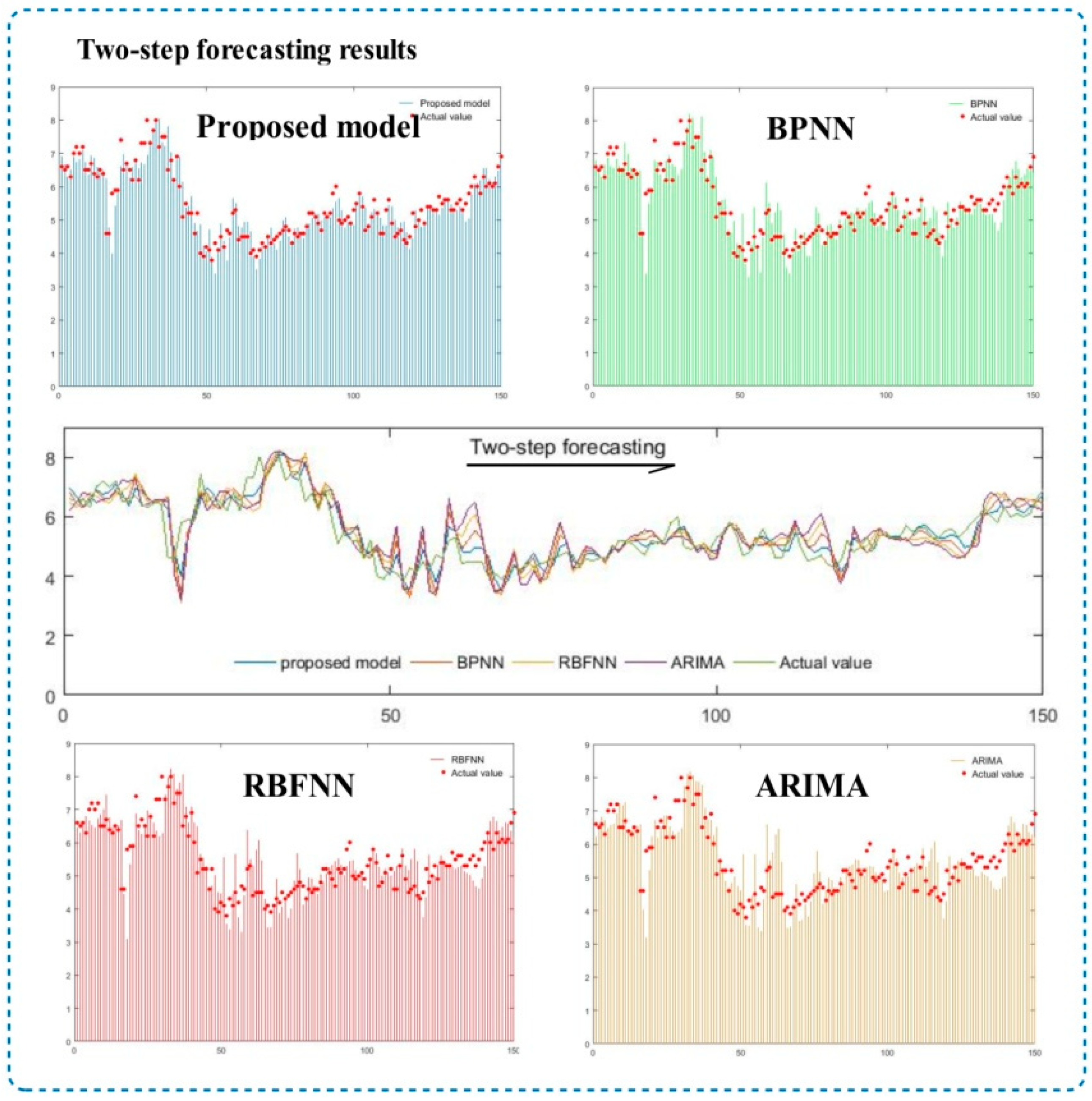
5.2. Multi-Step Forecasting

Multi-step forecasting is an effective way to test the accuracy of the forecasting method. Therefore, this paper employed multistep forecasting on the proposed hybrid model. The experimental results are used to verify the accuracy of the proposed approach. The results of the multi-step forecasting are presented in Table 6. Figure 5, Figure 6 and Figure 7 show the output values of different methods using multi-step forecasting. In 1-step ahead forecasting, the MAPE values of the BP, ARIMA, RBF, and the proposed model are 5.46%, 5.22%, 4.83%, and 3.07%, respectively. In 2-step ahead forecasting, the MAPE values of these models are 6.70%, 6.42%, 5.97%, and 4.55%. Additionally, in 3-step ahead forecasting, the MAPE values of the four models are 7.83%, 7.15%, 6.92%, and 5.46%, which indicates that the proposed hybrid model achieves a better performance than other conventional models.
When comparing the results of three-step forecasting with each other, one-step forecasting clearly performs better than the others.
Remark 4.
These results can be summarized as follows: The proposed hybrid approach obtains higher accuracy compared with the traditional models used in our experiments in both single step and multi-step forecasting. Therefore, the proposed hybrid approach is valid.

6. Discussion

This section discusses the sample selection, experimental results, which consist of each element in the proposed hybrid approach, the error evaluation indexes, and the forecast performance based on the DM (Diebold-Mariano) test and the Forecasting Effectiveness test.

6.1. Sample Selection

Currently, there is no explicit theory about how to select the number of training and testing sample. Too small and the input sample cannot train the model well, while too large and the sample will cause over-fitting. In terms of wind speed forecasting, how to select the number of input set is still a difficult and challenging issue [35,36]. It can only get the optimal input set by experiments. Besides, we organized and list the simulation results based on different ratio between training and testing samples in Table 7. Taking the one-step forecasting result of dataset one as an example, the MAPE values of the proposed model are 5.40%, 4.92%, 4.79%, 4.95%, and 5.11% when the ratio of training and testing sample is set to 7:3, 8:2, 9:1, 14:1, and 29:1, respectively. The forecasting accuracy of other ratios are all lower than the ratio 9:1′s accuracy. Table 1 below shows that the experiment we took before choosing a suitable ratio of training sample and testing sample. It can be indicated that when the ratio of training and testing sample is set to 9:1, the performance of wind speed forecasting outperforms the other ratios used in the experiment. Thus, based on the experiments and experience sample data are selected.

6.2. Forecasting Error Analysis

The proposed hybrid approach outperforms the conventional methods. The forecasting results and precision of the proposed model in four different wind turbines in multi-step forecasting are shown in Table 6. Then, Figure 5, Figure 6 and Figure 7 show the forecasting results of multi-step forecasting from the proposed approach and different traditional methods. The following conclusions are obtained from these results: (1) From the results of three-step forecasting, we can see that the hybrid method is more accurate than other conventional models because the error is the lowest many times. (2) The degree of fitting between the output series and the actual data from different models is shown in Figure 5, Figure 6 and Figure 7. The proposed approach is superior to the corresponding traditional methods, with a higher precision.
Multi-step forecasting is employed to further test the validity of the new hybrid approach. From Table 6, the results of multi-step forecasting of four wind turbines are shown. For wind turbine 1, the MAPE values of multi-step forecasting are 4.79%, 6.19%, and 10.14%, respectively. The other three wind turbines obtain similar results. As the results show, the new hybrid model is valid in multi-step forecasting.
Remark 5.
From the analysis, the performance of the hybrid method is better than those of the traditional models. The proposed model is able to adapt to the fluctuation of the input data so that it can obtain a more accurate result. Therefore, the new hybrid approach is more effective in wind speed prediction.

6.3. Validity of the Data Preprocessing Technique

The irregularity of the raw wind speed series often makes the input data contain high noise and fluctuation. Therefore, removing the noise from the original data is important to obtain a better forecasting accuracy. To test the validity of this data preprocessing technique, the results of the proposed model for four datasets using original and preprocessed data are listed together for comparison. From Table 2 and Table 3, the MAPE values of the proposed model decrease by 5.88%, 5.56%, 2.39%, and 7.36% in four wind turbines compared with the CSO-SVM model without the EEMD process. The MAE values also decreases by 0.1160, 0.0086, 0.2031, and 0.3109 in four wind turbines, respectively. The WI value increases by 0.0686, 0.0723, 0.0251, and 0.1565, respectively. The results indicate that the EEMD effectively improves the accuracy of the forecasting. As Table 2 and Table 3 show, all six metrics changed positively, and the results demonstrate that after reducing the noise of the raw data, the performance of the hybrid model improved significantly.

6.4. Significance of the Error Evaluation Indexes

Based on the results of six error evaluation indexes, namely MAPE, MAE, RMSE, WI, ENS, and ELM, the significance of the proposed hybrid model is estimated. Taking the forecasting results of dataset 2 as an example, the MAPE values of the proposed model, BPNN, RBFNN, and ARIMA are 3.07%, 5.42%, 6.41%, and 5.61%, respectively. The WI values are 0.9929, 0.9731, 0.9595, and 0.9752, respectively. Combining the results of these together, the hybrid model is proven to be superior to the traditional methods. In conclusion, the forecasting ability of the proposed model can be better analyzed with the help of these evaluation indexes, and the comparison between the proposed model and the other forecasting methods is more comprehensive.

6.5. Results of DM Test and Forecasting Effectiveness

Besides the error evaluation indexes, which have been applied to evaluate the forecasting ability of the proposed hybrid approach, this paper also used the DM (Diebold-Mariano) test and Forecasting Effectiveness to further study the forecasting accuracy.
In this paper, the DM test is used to study the significant differences in forecasting ability between the new hybrid model and some conventional methods. The results of the DM test are shown in Table 8. The DM statistical values far exceed the critical value at the 1% significance level, at which the value of | D M | is 2.1017. Thus, the proposed approach performs significantly different with the conventional methods at the 1% significance level. In conclusion, the proposed approach significantly outperforms the conventional methods.
The results of forecasting effectiveness is shown in Table 9. The first-order forecasting effectiveness is based on the expected value of the forecasting accuracy sequence, while the second-order forecasting effectiveness is related to the difference between the standard deviation and expectation of the forecasting accuracy sequence. In Table 8, the forecasting effectiveness of the proposed model outperforms all the other models in both first order and second order.

7. Conclusions

With a rapidly rising demand for clean energy obtained from renewable power resources, more attention and resources have been focused on the development of effectively utilizing these energy resources. Among those resources, wind power has the most promising future. In the area of the prediction, not only the accuracy, but also the stability, should be seen as key factors of the forecasting model. However, due to the uncertainty and intermittence of the raw wind speed data, the forecasting results obtained by conventional models cannot meet this goal. Additionally, with the poor results of forecasting, the power grids cannot make adjustments to the wind plan timely, causing low productivity and increasing the operation cost of the wind farms. Therefore, it is necessary to develop a short-term forecasting method that can achieve satisfactory accuracy and stability at the same time [37]. This paper suggests a new hybrid model that combines a parameter optimization algorithm (CSO) and a forecasting module (SVM). The key weight coefficients of the forecasting module are optimized by the proposed algorithm. To reduce the noise in the raw data, a data preprocessing technique (EEMD) is used to obtain a stationary time series. To verify the validity of the proposed model, multi-step ahead forecasting and several performance evaluation metrics are applied in this paper. Traditional forecasting methods are used for comparison. In one-step ahead forecasting, the MAPE values of the BP, ARIMA, RBF, and the proposed model are 5.46%, 5.22%, 4.83%, and 3.07%, respectively. In two-step ahead forecasting, the MAPE values of these models are 6.70%, 6.42%, 5.97%, and 4.55%, while in three-step ahead forecasting, the MAPE values of the four models are 7.83%, 7.15%, 6.92%, and 5.46%. Not only the figures of MAPE, but also other five variables and the two tests, show the excellent performance of the proposed approach. Based on the experimental results, the newly proposed approach achieved the highest performance in wind speed prediction in both one-step forecasting and multi-step forecasting, in comparison with the other three methods used in the experiment. In conclusion, based on the experimental results, the proposed approach achieved significant improvement in both forecasting accuracy and stability. The proposed a hybrid model, which effectively improved the accuracy and the stability of wind speed forecasting, can be a great tool in managing wind farms. Since this paper used the wind speed data from the power grids of China, the proposed model can adapt to the system smoothly, which can reduce the costs and risks of the power station. When employed in the dispatch of the power system, the proposed hybrid model can generate benefits economically. For instance, the wind station is able to make timely adjustments of the operating plan, and the accurate forecasting results can reserve the capacity of the wind farm, saving unnecessary costs, and avoiding generating waste. As for the focus of future studies, this proposed hybrid approach could be employed in other areas relating to trend forecasting, namely extreme weather prediction, profit forecasting, and traffic condition forecasting.

Author Contributions

Conceptualization, T.L.; Methodology, T.L.; Software, Y.G.; Validation, T.L. and J.H.; Formal Analysis, S.L.; Investigation, T.L.; Resources, S.L.; Data Curation, Y.G.; Writing-Original Draft Preparation, T.L.; Writing-Review & Editing, T.L.; Visualization, J.H.; Supervision, S.L.; Project Administration, S.L.

Conflicts of Interest

The authors declare no conflict of interest.

Abbreviation

VariablesMeaning
s(t)Raw data
ci(t)Residuals in raw data
rn(t)IMFs of the raw data
ε Amplitude of the added noise
ε n Standard deviation of the error
N ε Value of ensemble member
x i t + 1 New solution of cuckoo search
x i t Current solution of cuckoo search
αSize of each step in cuckoo search
Entry wise multiplications
L ( λ ) Lévy distribution
ϕ ( x ) Nonlinear mapping
wWeight vector of SVM
bScalar of SVM
C Penalty factor of the error
L ( x i , d i ) Loss function
C n 2 i = 1 n L ( x i , d i ) Empirical error
w 2 / 2 Regularization term
lQuantity of elements in the sample data series
α i ,   α i * Multipliers of Lagrange function
K ( x , x i ) Kernel function of SVM
γParameter of the kernel function
NTotal output samples
y i Actual series
y p i Predicting results

References

  1. Salcedo-Sanz, S.; Pérez-Bellido, Á.M.; Ortiz-García, E.G.; Portilla-Figueraa, A.; LuisPrieto, L.; Correosoc, F. Accurate short-term wind speed forecasting by exploiting diversity in input data using banks of artificial neural networks. Neurocomputing 2009, 72, 1336–1341. [Google Scholar] [CrossRef]
  2. Soman, S.S.; Zareipour, H.; Malik, O.; Mandal, P. A review of wind power and wind speed forecasting methods with different time horizons. In Proceedings of the North American Power Symposium 2010, Arlington, TX, USA, 26–28 September 2010. [Google Scholar]
  3. Wang, J.; Heng, J.; Xiao, L.; Wang, C. Research and application of a combined model based on multi-objective optimization for multi-step ahead wind speed forecasting. Energy 2017, 125, 591–613. [Google Scholar] [CrossRef]
  4. Mohandes, M.A.; Halawani, T.O.; Rehman, S.; Hussaina, A.A. Support vector machines for wind speed prediction. Renew. Energy 2004, 29, 939–947. [Google Scholar] [CrossRef]
  5. Liu, H.; Tian, H.-Q.; Chen, C.; Li, Y. A hybrid statistical method to predict wind speed and wind power. Renew. Energy 2010, 35, 1857–1861. [Google Scholar] [CrossRef]
  6. Liu, H.; Tian, H.Q.; Pan, D.F.; Li, Y.F. Forecasting models for wind speed using wavelet, wavelet packet, time series and artificial neural networks. Appl. Energy 2013, 107, 191–208. [Google Scholar] [CrossRef]
  7. Li, G.; Shi, J. On comparing three artificial neural networks for wind speed forecasting. Appl. Energy 2010, 87, 2313–2320. [Google Scholar] [CrossRef]
  8. Barbounis, T.G.; Theocharis, J.B.; Alexiadis, M.C.; Dokopoulos, P.S. Long-term wind speed and power forecasting using local recurrent neural network models. IEEE Trans. Energy Convers. 2006, 21, 273–284. [Google Scholar] [CrossRef]
  9. Cheng, C.H.; Wei, L.Y. A novel time-series model based on empirical mode decomposition for forecasting TAIEX. Econ. Model. 2014, 36, 136–141. [Google Scholar] [CrossRef]
  10. Zhou, J.Y.; Shi, J.; Li, G. Fine tuning support vector machines for short-term wind speed forecasting. Energy Convers. Manag. 2011, 52, 1990–1998. [Google Scholar] [CrossRef]
  11. Liu, D.; Niu, D.X.; Wang, H.; Fan, L. Short-term wind speed forecasting using wavelet transform and support vector machines optimized by genetic algorithm. Renew. Energy 2014, 62, 592–597. [Google Scholar] [CrossRef]
  12. Hu, Q.H.; Zhang, S.G.; Xie, Z.X.; Mi, J.S.; Wan, J. Noise model based v-support vector regression with its application to short-term wind speed forecasting. Neural Netw. 2014, 57, 1–11. [Google Scholar] [CrossRef] [PubMed]
  13. Guo, Z.H.; Wu, J.; Lu, H.Y.; Wang, J.Z. A case study on a hybrid wind speed forecasting method using BP neural network. Knowl.-Based Syst. 2011, 24, 1048–1056. [Google Scholar] [CrossRef]
  14. Guo, Z.H.; Zhao, J.; Zhang, W.Y.; Wang, J.Z. A corrected hybrid approach for wind speed prediction in Hexi Corridor of China. Energy 2011, 36, 1668–1679. [Google Scholar] [CrossRef]
  15. Pourmousavi Kani, S.A.; Aredhali, M.M. Very short-term wind speed prediction: A new artificial neural network-Markov chain model. Energy Convers. Manag. 2011, 52, 738–745. [Google Scholar] [CrossRef]
  16. Pourmousavi Kani, S.A.; Riahy, G.D.; Mazhari, D. An innovative hybrid algorithm for very short-term wind speed prediction using linear prediction and markov chain approach. Int. J. Green Energy 2011, 8, 147–162. [Google Scholar] [CrossRef]
  17. Liu, H.; Chen, C.; Tian, H.Q.; Li, Y.F. A hybrid model for wind speed prediction using empirical mode decomposition and artificial neural networks. Renew. Energy 2012, 48, 545–556. [Google Scholar] [CrossRef]
  18. Mohammadi, A.; Dehghani, M.J.; Ghazizadeh, E. Game Theoretic Spectrum Allocation in Femtocell Networks for Smart Electric Distribution Grids. Energies 2018, 11, 1635. [Google Scholar] [CrossRef]
  19. Kianoosh, G.; Boroojeni, M.; Hadi, A.; Bahrami, S.S.; Iyengar, A.I.; Sarwat, O.K. A novel multi-time-scale modeling for electric power demand forecasting: From short-term to medium-term horizon. Electr. Power Syst. Res. 2017, 142, 58–73. [Google Scholar]
  20. Haque, A.U.; Mandal, P.; Kaye, M.E.; Meng, J.L.; Chang, L.C.; Senjyu, T. A new strategy for predicting short-term wind speed using soft computing models. Renew. Sustain. Energy Rev. 2012, 16, 4563–4573. [Google Scholar] [CrossRef]
  21. Li, G.; Shi, J. On comparing three artificial neural networks for wind speed forecasting. Appl. Energy 2010, 87, 2313–2320. [Google Scholar]
  22. Ortiz-García, E.G.; Salcedo-Sanz, S.; Perez-Bellido, A.M.; Gascon-Moreno, J.; Portilla-Figueras, J.A.; Prieto, L. Short-term wind speed prediction in wind farms based on banks of support vector machines. Wind Energy 2011, 14, 193–207. [Google Scholar]
  23. Xiao, L.; Wang, J.; Hou, R.; Wu, J. A combined model based on data pre-analysis and weight coefficients. optimization for electrical load forecasting. Energy 2015, 82, 524–549. [Google Scholar] [CrossRef]
  24. Vapnik, V. Statistical Learning Theory, 2nd ed.; Wiley: New York, NY, USA, 1998. [Google Scholar]
  25. Vapnik, V. The Nature of Statistical Learning Theory; Springer: New York, NY, USA, 1999. [Google Scholar]
  26. Wu, Z.; Huang, N.E. Ensemble empirical mode decomposition: A noise-assisted data analysis method. Adv. Adapt. Data Anal. 2009, 1, 1–41. [Google Scholar] [CrossRef]
  27. Yang, X.S.; Deb, S. Engineering optimization by cuckoo search. Int. J. Math. Model. Numer. Optim. 2010, 1, 330–343. [Google Scholar]
  28. Yang, W.; Wang, J.; Wang, R. Research and application of a novel hybrid model based on data selection and artificial intelligence algorithm for short term load forecasting. Entropy 2017, 19, 52. [Google Scholar] [CrossRef]
  29. Yang, X.S.; Deb, S. Cuckoo search via Lévy flights. Presented at 2009 World Congress on Nature & Biologically Inspired Computing (NaBIC), Coimbatore, India, 9–11 December 2009. [Google Scholar]
  30. Pai, P.; Lin, C. A hybrid ARIMA and support vector machines model in stock price forecast. Omega 2005, 33, 497–505. [Google Scholar] [CrossRef]
  31. Huang, C.; Davis, L.; Townshend, J. An assessment of support vector machines for land cover classification. Int. J. Remote Sens. 2002, 23, 725–749. [Google Scholar] [CrossRef]
  32. Sung, A.H.; Mukkamala, S. Identifying important features for intrusion detection using support vector machines and neural networks. In Proceedings of the 2003 Symposium on Applications and the Internet, Orlando, FL, USA, 27–31 January 2003. [Google Scholar]
  33. Xiao, L.; Shao, W.; Wang, C.; Zhang, K.; Lu, H. Research and application of a hybrid model based on multi-objective optimization for electrical load forecasting. Appl. Energy 2016, 180, 213–233. [Google Scholar] [CrossRef]
  34. Iversen, E.B.; Morales, J.M.; Møller, J.K.; Madsen, H. Short-term probabilistic forecasting of wind speed using stochastic differential equations. Int. J. Forecast. 2015, 32, 981–990. [Google Scholar] [CrossRef]
  35. Chao, R.; Ning, A.; Wang, J.Z.; Li, L.; Hu, B.; Shang, D. Optimal parameters selection for BP neural network based on particle swarm optimization: A case study of wind speed forecasting. Knowl.-Based Syst. 2014, 56, 226–239. [Google Scholar]
  36. Wang, J.; Zhu, S.; Zhao, W.; Zhu, W. Optimal parameters estimation and input subset for grey model based on chaotic particle swarm optimization algorithm. Expert Syst. Appl. 2011, 38, 8151–8158. [Google Scholar] [CrossRef]
  37. Zhou, J.Z.; Sun, N.; Jia, B.J.; Peng, T. A Novel Decomposition-Optimization Model for Short-Term Wind Speed Forecasting. Energies 2018, 11, 1752. [Google Scholar] [CrossRef]
Figure 1. The flowchart of the Cuckoo Search Algorithm.
Applsci 08 01754 g001
Figure 2. The flowchart of the proposed forecasting method.
Applsci 08 01754 g002
Figure 3. The original wind speed data and de-noised data from four datasets.
Applsci 08 01754 g003
Figure 4. Wind speed data noise reduction using EEMD preprocessing process.
Applsci 08 01754 g004
Figure 5. One-step forecasting results of the proposed model and other traditional models (BP RBF ARIMA).
Applsci 08 01754 g005
Figure 6. Two-step forecasting results of the proposed model and other traditional models (BP RBF ARIMA).
Applsci 08 01754 g006
Figure 7. Three-step forecasting results of the proposed model and other traditional models (BP RBF ARIMA).
Applsci 08 01754 g007
Table 1. The description of the error evaluation indexes.
MetricDefinitionEquation
MAEThe mean absolute error of N forecasting results MAE = 1 N i = 1 N | y p i y i |
MAPEThe average of N absolute percentage error MAPE = 1 N i = 1 N | y p i y i y i | × 100 %
RMSEThe square root of the average of the error square RMSE = 1 N i = 1 N ( y p i y i ) 2
WIWillmott’s Index WI = 1 [ i = 1 N ( y p i y i ) 2 i = 1 N ( | y p i y ¯ | + | y i y ¯ | ) 2 ] , 0 WI 1
ENSNash-Sutcliffe coefficient E NS = 1 [ i = 1 N ( y p i y i ) 2 i = 1 N ( y i y ¯ ) 2 ] , E NS 1
ELMLegates and McCabe Index E LM = 1 [ i = 1 N | y i y p i | i = 1 N | y i y ¯ | ] , E LM 1
Table 2. Comparison of the value of RMSE, MAE, and MAPE between the proposed model and some related models.
ModelRMSEMAE MAPE (%)RMSEMAE MAPE (%)
Wind turbine 1 Wind turbine 3
EEMDCSOSVM0.35130.18154.790.24630.21202.69
EEMDPSOSVM0.46520.21595.630.30270.24362.82
CSOSVM0.82940.297510.670.51210.42515.08
PSOSVM1.01350.710012.180.79280.63629.70
Wind turbine 2 Wind turbine 4
EEMDCSOSVM0.23420.18413.070.26790.30283.91
EEMDPSOSVM0.27440.21913.240.31470.18694.44
CSOSVM1.13810.19277.630.92040.61379.27
PSOSVM0.66800.51658.581.14780.819010.15
Table 3. Comparison of the value of WI, ENS, and ELM between the proposed model and some related models.
ModelWIENSELMWIENSELM
Wind turbine 1 Wind turbine 3
EEMDCSOSVM0.98380.93320.76000.99180.96700.8268
EEMDPSOSVM0.97230.92510.71480.97440.93100.7201
CSOSVM0.91520.68580.44600.96670.87200.6525
PSOSVM0.86220.53670.35990.82390.49500.1197
Wind turbine 2 Wind turbine 4
EEMDCSOSVM0.99290.97130.83880.98390.93500.7565
EEMDPSOSVM0.98760.94240.79500.97860.92340.7159
CSOSVM0.92060.70110.51340.82740.48850.2514
PSOSVM0.91740.68520.48120.74900.33550.1253
Table 4. Comparison of the value of RMSE, MAE, and MAPE between the proposed model and some traditional models (BP RBF ARIMA).
ModelRMSEMAE MAPE (%)RMSEMAEMAPE (%)
Wind turbine 1 Wind turbine 3
BPNN0.59390.49848.680.47940.32865.28
RBFNN0.88670.592410.320.65870.44686.52
ARIMA0.57840.46728.410.44720.29075.13
EEMDCSOSVM0.35130.18154.790.24630.21202.69
Wind turbine 2 Wind turbine 4
BPNN0.39980.32325.420.45850.33856.34
RBFNN0.48470.38066.411.23740.554310.32
ARIMA0.36270.29255.610.41220.36795.88
EEMDCSOSVM0.23420.18413.070.26790.30283.91
Table 5. Comparison of the value of WI, ENS and ELM between the proposed model and some traditional models (BP RBF ARIMA).
ModelWIENSELMWIENSELM
Wind turbine 1 Wind turbine 3
BPNN0.94100.78220.54030.97080.88500.6806
RBFNN0.89260.60170.46300.94290.77510.6128
ARIMA0.94760.81370.65120.97550.90240.7148
EEMDCSOSVM0.98380.93320.76000.99180.96700.8268
Wind turbine 2 Wind turbine 4
BPNN0.97310.88890.69620.94120.76280.5877
RBFNN0.95950.83200.64220.70350.33390.3248
ARIMA0.97520.89330.70170.95030.79370.6128
EEMDCSOSVM0.99290.97130.83880.98390.93500.7565
Table 6. Results of multi-step forecasting of the proposed model.
Dataset MAEMAPE (%)RMSEWIENSELM
Dataset 11-Step0.18154.790.35130.98380.93320.7600
2-Step0.36226.190.45460.97200.88740.6699
3-Step0.589510.140.73540.92490.71150.4609
Dataset 21-Step0.18413.070.23420.99290.97130.8388
2-Step0.39626.530.50340.95830.83550.6310
3-Step0.657910.700.82910.88870.60730.3925
Dataset 31-Step0.21202.690.24630.99180.96700.8268
2-Step0.48145.97053080.95290.83060.5820
3-Step0.86949.520.83290.85990.57050.3240
Dataset 41-Step0.30283.910.26790.98390.93500.7565
2-Step0.42755.120.36520.96450.86040.6667
3-Step0.53108.030.54370.91890.68830.4797
Table 7. MAPE (%) values of different ratios between training and testing sample of the proposed model.
DataseForecasting StepsRaito Between the Training Sample and Testing Sample (MAPE (%))
7:38:29:114:129:1
Dataset 11-step5.404.924.794.955.11
2-step9.578.156.198.828.97
3-step13.9413.4610.1414.8415.73
Dataset 21-step4.163.913.073.543.76
2-step9.327.526.537.328.44
3-step12.6911.2410.7011.1511.80
Dataset 31-step3.483.282.693.413.97
2-step6.626.125.976.156.72
3-step10.739.829.529.8410.15
Dataset 41-step4.884.093.914.164.51
2-step7.266.655.125.525.84
3-step11.0110.398.038.858.99
Table 8. Results of DM test.
Datasets BPNNRBFNNARIMA
Dataset 11-step7.28597.43928.0205
2-step6.80737.16827.5217
3-step6.52706.94637.2258
Dataset 21-step6.94697.42456.2829
2-step6.77167.28396.5691
3-step6.83587.14756.2039
Dataset 31-step7.13256.21616.2934
2-step7.04136.47556.7390
3-step6.94276.35866.4803
Dataset 41-step6.89417.27907.1783
2-step7.25647.23877.0492
3-step6.43966.92576.5864
Table 9. Forecasting Effectiveness of different models for four datasets.
Dataset BPNNRBFNNARIMAEEMDCSOSVM
Dataset 1First order0.89510.88890.88740.9146
Second order0.83220.82570.82830.8638
Dataset 2First order0.91300.90290.90720.9367
Second order0.83840.83620.84360.8842
Dataset 3First order0.92830.91770.92200.9409
Second order0.85170.85820.86250.8975
Dataset 4First order0.89560.89340.90310.9269
Second order0.83440.83600.84920.8816

