Registration of Dental Tomographic Volume Data and Scan Surface Data Using Dynamic Segmentation

Abstract

Over recent years, computer-aided design (CAD) has become widely used in the dental industry. In dental CAD applications using both volumetric computed tomography (CT) images and 3D optical scanned surface data, the two data sets need to be registered. Previous works have registered volume data and surface data by segmentation. Volume data can be converted to surface data by segmentation and the registration is achieved by the iterative closest point (ICP) method. However, the segmentation needs human input and the results of registration can be poor depending on the segmented surface. Moreover, if the volume data contains metal artifacts, the segmentation process becomes more complex since post-processing is required to remove the metal artifacts, and initially positioning the registration becomes more challenging. To overcome these limitations, we propose a modified iterative closest point (MICP) process, an automatic segmentation method for volume data and surface data. The proposed method uses a bundle of edge points detected along an intensity profile defined by points and normal of surface data. Using this dynamic segmentation, volume data becomes surface data which can be applied to the ICP method. Experimentally, MICP demonstrates fine results compared to the conventional registration method. In addition, the registration can be completed within 10 s if down sampling is applied.

1. Introduction

In the dental computer-aided design and computer-aided manufacturing (CAD/CAM) industry, volumetric computed tomography (CT) images and scan surfaces are most commonly used. However, the two data types are very different, because their measurement techniques fundamentally differ. The volume data contains intensity information of the internal organs of the human body, while the surface data contains only the visible surfaces, that is, the teeth and the gingiva. Because of their different features, volume data and surface data are used for different dental applications. However, there are many applications which require both volume data and surface data and for the accurate registration of the volume and surface data is necessary. To achieve this we propose a novel registration method of volume data and surface data.

1.1. Backgrounds

1.1.1. Volumetric Computed Tomography (CT) Data

Volumetric computed tomography (CT) data features a voxel structure, with each voxel having an intensity value. The standard data format for this volume data is the Digital Imaging and Communications in Medicine (DICOM) format, which contains more than 90 valuable information fields such as intensity values, patient details, modality, and manufacturer, acquisition data, and so on [1,2,3]. The volume data is obtained by X-ray computed tomography (CT) scanning. In practice, the volume data is divided into three parallel planes, the sagittal, axial, and coronal planes, and is used in the analysis of many operations. For dental applications, cone beam computed tomography (CBCT) is used [4,5,6]. While a ‘fan-shaped’ X-ray beam is used in medical CT, a ‘cone’ X-ray beam is used in cone beam CT. Because medical CT features higher X-ray exposure than CBCT, the resolution of the volume data provided by medical CT is higher than that provided by CBCT [7]. However, CBCT is used in many fields of dentistry due to the low X-ray exposure associated with it. Also, CBCT data is much easier to use with 3D interpolation since, due to its X-ray geometry, it forms isotropic voxels, whereas medical CT forms anisotropic voxels.

1.1.2. Dental Surface Data

3D scanners are well established and widely used in industry and dental 3D scanners, which are optimized to scan plaster models, are also widely used in dentistry. The standard data format for the surface data is standard triangle language (STL) [8] and polygon file format (PLY). This surface data contains vertices, faces, normal vectors, and so on. To obtain the surface data, 3D optical scanners using structured light are generally used because they are fast and precise [9,10]. The 3D optical scanner is composed of two cameras for epipolar geometry and one projector for pattern projection. The surface data features much better resolution and accuracy than the volume data.

1.2. Related Works

Volume data and surface data have different features and there are various dental CAD/CAM applications which use both volume and surface data. Therefore, the registration of volume data and surface data is necessary.

Before approaching the registration problem, the intrinsic errors of each data should be considered numerically. 3D dental scanners (Identica Blue, MEDIT Corp., Seongbuk-gu, Seoul, Korea) are accurate to 0.007 mm. However, considering the whole process of making the impression and the plaster model for measurement, the total intrinsic error of the surface data is around 0.06 mm in practice [11,12]. On the other hand, the accuracy of CBCT (MercuRay, HITACHI, Chiyoda, Japan) is approximately 0.20 mm [13]. Dental prostheses cannot be designed using CBCT volume data because of this relatively low accuracy. Thus, the intrinsic error of the scan-derived data is generally negligible and only that of the volume data is a cause for concern.

Usually the registration problem concerns the same types of data and that is the basic premise in 2D images or 3D data registration. However, the registration problem in this paper concerns different types of data, volume data and surface data. Data must be converted to identical data types before the registration process, and most previous works convert the volume data to surface data. This type of conversion process that extracts dental surface data from volume data is called segmentation. Surface data registration can be performed on the resulting segmented dental surface data. Generally, surface registration is done by the iterative closest point (ICP) method, which needs good initial conditions [14,15,16,17] and is widely used in the dental CAD/CAM industry. The flow chart for the ICP method is shown in Figure 1.

Although the established registration framework (ICP) is currently used clinically for dental applications, some drawbacks still exist; the requirement of human inputs and the metal artifact problem.

Human input is needed to set the initial positioning. Although there is much research on global registration, which obtains the initial conditions automatically for ICP, applying this algorithm to dental model registration is challenging because dental surface data suffers from ambiguity due to teeth shape characteristics [18]. Segmentation also requires human input. The most commonly used segmentation methods are thresholding, region growing, and active contour methods such as a level set. Thresholding is the most straightforward and basic segmentation method and teeth volume data is segmented by giving lower and upper intensity values [19]. The region growing method starts with a set of seed points and regions are grown based on the similarity of intensity [20,21]. Level set segmentation is performed using 2D axial direction sliced images and stacked for a 3D segmentation result [22,23,24]. To improve the result of segmentation, combining the above segmentation methods has also been studied [25]. However, every segmentation method mentioned above needs a human input; lower and upper threshold values must be defined for thresholding segmentation, seed points must be defined for region growing segmentation, and initial contours must be defined for level set segmentation. In the established framework for the registration of volume and surface data, this human input stage for segmentation represents the most time-consuming step. Although some automatic tooth segmentation methods have been studied, each study has constraints and cannot be used in a wide variety of applications [26,27]. Also, once the segmentation has been done, post processing, such as surface smoothing and island removing, is required. The result of segmentation may even differ from person to person.

Another drawback of the established registration procedure is the metal artifact problem [28]. If a patient has a prosthetic appliance made of metal, the volume data is seriously affected by white saturation. The quality of the resulting segmented surface is also affected. Initial conditioning for ICP also becomes more difficult because non-artifact points on the segmented surface must be selected manually. Many studies have considered the metal artifact problem [29,30] but they have resulted in a reduction rather than an elimination of the metal artifact effect so the problem remains unsolved.

1.3. Motivation and Contribution of the Thesis

ICP is the most useful fine registration algorithm and produces accurate results. However, volume data is composed of voxel structures with intensity values and contains no points or normal data. To find corresponding points between volume and surface data to apply to ICP, point data should be segmented from the volume data. In the established registration procedure, the segmented surface is used as a target surface for the ICP algorithm. Hence, the previous works must make considerable effort to ensure good quality segmented surface data, and this requires human input. We are motivated to try and overcome this fundamental limitation of the established registration procedure. Registration does not require fully segmented surface information, but only the corresponding points for the ICP method. Obtaining these points has proven the most challenging step in previous works on segmentation. The proposed method, the modified iterative closest point (MICP) obtains the corresponding points by dynamic segmentation defined by an intensity profile analysis. The remainder of this paper is organized as follows. In Section 2 detailed explanations of the proposed method are given. In Section 3 the results of the proposed method are shown and a comparison of its effectiveness with that of the established method is provided. Finally, the concluding remarks of the paper are given in Section 4.

2. Proposed Method: MICP

2.1. Overview

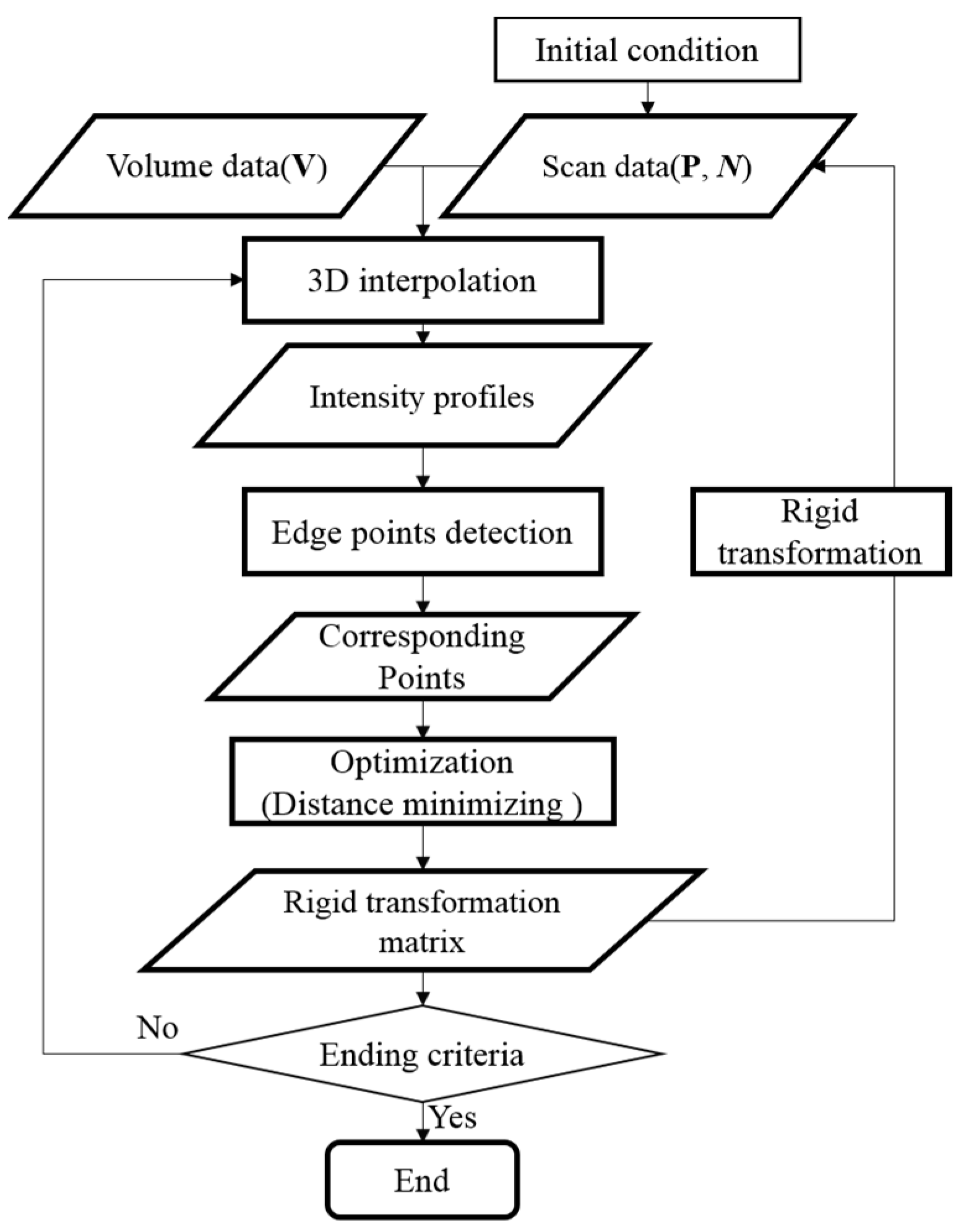
The overall process of the algorithm can be written in pseudo-code as follows:

Pseudo-code: The overall process of the proposed method

Data: $\mathrm{V},\mathrm{P}$ Result: $T_f$ while (e < ending criteria) $\left\{V^{\prime }\right\}$ ← interpolation(V) {E} ← step_edge(V) {M} ← match(E,P′,N) $\left\{T_{init}\right\}$ ← minimizing point-to-plane distance metric $\left\{P^{\prime }\right\}$ ← {$T_{init}$P} end $\left\{T_f\right\}\leftarrow ICP\left(T_{init}·P_s,P_t\right)$

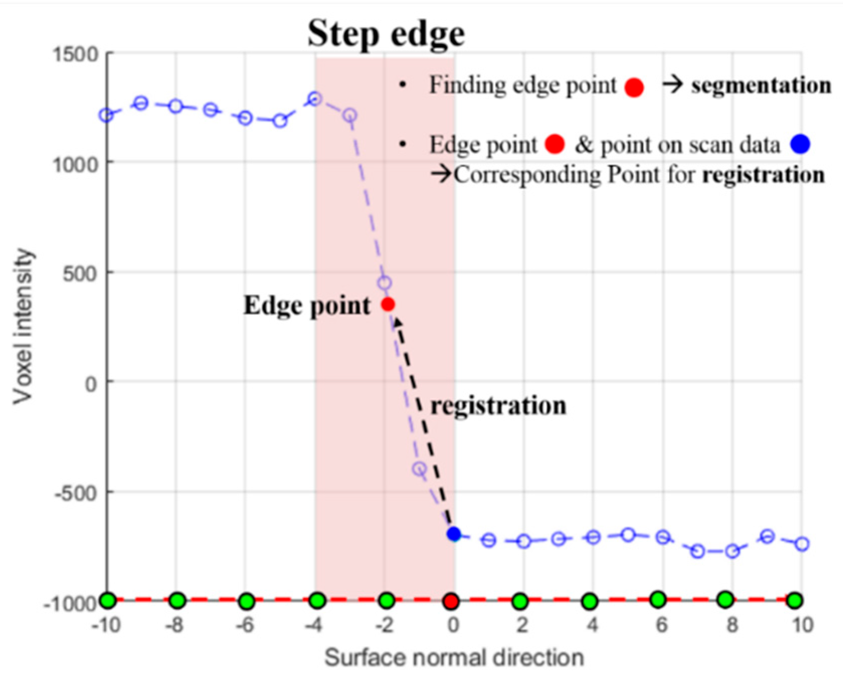
To align the volume data (V) and the scan data (P), the two were initially manually placed proximally. For a single point and normal vector from the surface data, an intensity profile can be defined in the volume data. The intensity profile has several new points aligned with the normal vector to the surface data. These points are defined with uniform intervals and new intensity values are given to these points by 3D interpolation (V′). Because the volume data and surface data are initially positioned well, a single intensity step edge is apparent in the intensity profile (Figure 2).

The step edge represents the boundary of the teeth in the volume data and provides valuable information for both segmentation and registration. For most existing segmentation algorithms that extract surface data from volume data, points of the segmented surface must be positioned in the step edge(E). In other words, an edge point on an intensity profile should relate directly to a 3D segmented point. From the registration aspect, if the volume data and scan data are aligned properly, this step edge point must converge to the origin (x = 0).

The intensity profile is calculated for every point so the step edge can be determined. If the step edge exists in the intensity profile, the interpolated edge point in the 3D vertex can be obtained and the edge point becomes a segmented point. These points are the corresponding points used for the ICP algorithm (M). The rigid transformation matrix can be calculated by minimizing the distance between the matching points. If the average distance between the two data sets becomes less than the ending criteria, the dynamic segmentation process terminates.

Unlike the previous methods that use only volume data for segmentation, we use both volume data and surface data. The proposed registration procedure does not need any human input except for initial positioning and works automatically. In addition, the proposed method uses the edge points of the teeth. Therefore, it is robust to the artifact problem. The overall flow chart of the proposed registration procedure is shown in Figure 3.

2.2. Automatic Registration Process

2.2.1. Defining an Edge Point on Intensity Profile

Based on a single point of scan data, an intensity profile can be generated along the normal direction of the point by 3D interpolating with a uniform interval. For this intensity profile generating process, two parameters are needed, the maximum distance and the interval. In this study, we used 10 voxels as the maximum distance and 1 voxel as the interval, and a total of 21 interpolation values are calculated for 1 intensity profile. With this intensity profile, the presence of step edges can be determined. The first derivative of the line profile can be used to determine the presence of a step edge. The determined step edge could correspond to an intensity increasing shape or an intensity decreasing shape.

Because the normal direction of the surface data and the gradient direction of the volume data are opposite, the sign of the first gradient of the step edge must be negative. In conclusion, if an intensity profile has a high negative value for the first derivatives, that intensity profile has a step edge and the point of the surface data becomes a corresponding point for ICP. Then, the minimum value of the first derivatives is defined. Many studies have evaluated the HU values of materials in CBCT volume data [31,32,33,34]. There are two step edges which define the teeth boundaries, whether bone—air or bone—skin. To detect and use both step edges, the step edge defined by the relatively low first derivatives value, the bone—skin value, becomes the reference. Based on the previous studies, −800 was defined as a reasonable slope value of the first derivatives for defining the step edge [19]. All experiments in Section 3 used this slope value to define step edges. This edge point is physically the same as a zero-crossing edge point [35]. The detected edge point on the intensity profile is a 3D point because the intensity profile is defined by 3D interpolation from volume data.

Volume data is highly complex data containing not only teeth, but also bones and tissues. Therefore, more than two step edges could be found. These intensity profiles are not used for the registration process. The proposed registration works based on only the defined points of surface data which are near the step edges. Because of this strict standard, the proposed registration method is robust to cases with metal artifacts.

Once the edge point is found, the sub-voxel level edge point is defined by local 3D interpolation back and forth along the intensity profile. This is the final step for a single intensity profile. The sub-voxel level edge point becomes a corresponding point to the point defining the intensity profile.

2.2.2. Dynamic Segmentation

For a single point on the surface data, a corresponding point in the volume data can be found by intensity profile analysis. If this intensity profile analysis is applied to all points on the surface data, a set of corresponding points for ICP can be obtained. The surface data and volume data are initially positioned. All detected edge points can be visualized as surface data. This surface data is a segmented surface representing the tooth volume data and can be a corresponding point for ICP. In the proposed method, if correspondence is obtained, the conventional ICP step for finding corresponding points becomes unnecessary. Now, points with edge points are set as moving surface data and the segmented points are set as the target surface data. Then, the sum of the distance between the corresponding points is minimized using the singular value decomposition (SVD) method and a rigid transformation matrix can be obtained [36]. The moving surface data is transformed by the obtained transformation matrix in a process which is a single iteration process under the proposed procedure. Even if the data is down-sampled, ICP still uses several thousands of points for which it needs to find correspondences. Repeating SVD iteratively increases the computational costs of ICP. In contrast, the proposed algorithm uses only hundreds of points from the interpolated data and already knows the correspondences. Therefore, the computational costs incurred by using SVD are substantially lower than those of ICP.

This whole process is performed iteratively just the same as for the conventional iterative closest point algorithm. The procedure of the established registration method for volume data and surface data uses only one segmented surface data. However, the proposed registration method includes the segmentation process within the iteration which is why this segmentation method is termed ‘dynamic’ segmentation. The segmented surface used as the target surface differs every iteration. For the proposed dynamic segmentation method using intensity profile analysis, the volume data can be used directly as input data. Above all, the dynamic segmentation works automatically without needing any human input. During the iteration process, the edge point on the intensity profile gets closer to the point on the surface.

2.3. Factors to Consider in Proposed Method

2.3.1. Normal Correction

Fundamentally, the 3D vertex points are the raw data obtained from the 3D scanning and are not positioned regularly due to the geometry of the model. From this point cloud, a mesh model is generated from various meshing algorithms and a surface normal can be calculated. From the near surface normal directions of a point, a vertex normal can be calculated. However, the mesh model generated from raw scan data is not good mesh data because of its point irregularity. There are many long-edge triangle faces on the raw mesh data and the calculated normal data is noisy. The dynamic segmentation that is proposed for MICP is sensitive to the normal direction of the scan data. Using raw scan data works fine but more accurate registration results can be achieved by correcting the normal data. There are two ways to correct normal data, normal smoothing and remeshing [37,38]. Normal smoothing can remove the high-frequency noise in the normal data and generates more reliable intensity profiles. However, the input normal for smoothing is basically inaccurate because of the irregular mesh data from the raw point cloud data. To overcome the irregularity, we remeshed the mesh data. After remeshing from the original mesh data with equal edge lengths, points on the surface are realigned and regular mesh data is generated (Figure 4). More accurate face normal data can be calculated from the regular mesh data and more accurate vertex normal data can be obtained sequentially.

2.3.2. Length Value to Generate Intensity Profile

To generate the intensity profile through point normal direction, a limitation length should be set before the process. To achieve accurate registration, a proper length value is needed. If the intensity profile is set to a short length value, no edge points can be detected and registration cannot be performed because there is no correspondence between the scan data and the CBCT volume data. Alternatively, if the intensity profile is set to a long length value, unintended edge points can be detected and wrong correspondences lead to inaccurate registration results. Edge points of gums, tissue regions or metal artifact regions can be ignored automatically by the proper length value. With the proper distance value, the edge points of teeth regions are segmented and can be used to achieve good correspondences.

2.3.3. Down Sampling

One of the differences between volume data and surface data is their resolution. Surface data have a much higher resolution than CBCT volume data. The resolution of volume data is not as high as that of surface data even if 3D interpolated intensity values are given to all the points. A voxel in the volume data may even correspond to more than dozens of points in the surface data. Thus, using all points of the surface data is ineffective. To improve the efficiency of MICP registration, input surface data was down sampled to match the volume data. The conventional registration process, always contains a segmentation process that takes at least 20 min, so the expected time reduction is low. However, the expected elapsed time of the proposed registration method is dramatically lowered because segmentation is contained in the iteration. Generally, there are 4 down sampling algorithms that are widely used in 3D data handling; uniform sampling, random sampling, normal sampling, and covariance sampling [39]. The volume data has uniform resolution along the x, y, and z directions. Given this feature of the volume data, it is reasonable to use uniform sampling to adjust the resolution of the input data.

3. Results & Discussion

In this chapter, the experimental results of MICP are presented. Also, the proposed method is compared to the conventional registration method in terms of the average distance of points (D value). The proposed algorithm was implemented in MATLAB R2017a (The MathWorks Inc., Natick, MA, USA) on a personal computer with an i7-4770K processor with 8GB memory and a Windows 7 operating system (Microsoft Cop., Redmond, Washington, DC, USA). To visualize the results, MITK 2016.11.0 [40] and Meshlab 2016 [41] software were used.

3.1. Result

3.1.1. Data Sets

To be able to register the CBCT volume data and the dental scan surface data, naturally both data types should be obtained from the same patient. To obtain the experimental result, four sets of volume data and surface data were used for the registration (Figure 5). The volume data were obtained from CBCT (CB MercuRay, HITACHI, Chiyoda, Japan) and the surface data was obtained from a 3D optical dental scanner (Identica blue, MEDIT Corp., Seongbuk-gu, Seoul, Korea). The dimension of all volume data is 512 × 512 × 512. The pixel spacing of the volume data of set1 and set2 is 0.2920 and of set3 and set4 is 0.2.

3.1.2. Registration by the Conventional Method

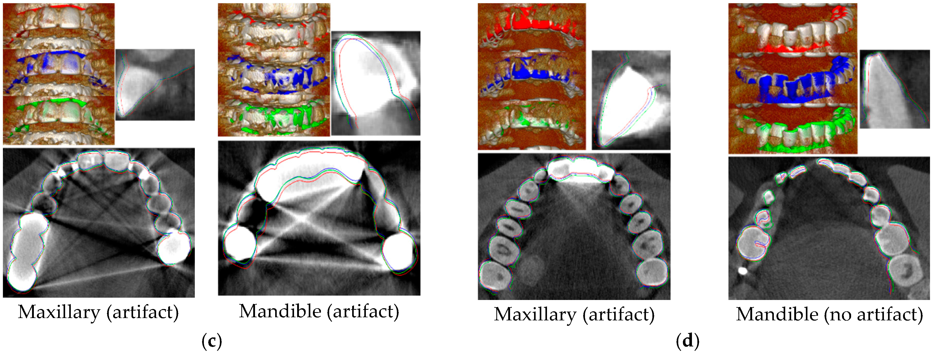
Although there is no ground truth for the registration result of volume data and scan data, conventional registration using segmentation and the iterative closest point has been used in the dental field for a long time. Therefore, to compare registration performance, the ground truth used was the result of conventional registration. For the comparison, the conventional registration process was performed on all input data sets. The region of interest (ROI) was set to the teeth region in the CBCT volume data. In the ROI, thresholding and region growing was performed for segmentation. After the volume data has been segmented, the segmented region is extracted as surface mesh data. Then, human input is used to select a 3-point pair for the initial condition. ICP is performed as the last registration step. The result of ICP is shown in Figure 6 and

Table 1. The result of conventional registration.

Input Data		Metal Artifact	${\mathit{E}}_{\mathit{ICP}}$ (mm)	$\mathit{S}{\mathit{D}}_{\mathit{ICP}}$ (mm)
Set no.1	Maxillary	No	0.3612	0.1308
	Mandible	No	0.3357	0.1140
Set no.2	Maxillary	Yes	0.4170	0.1574
	Mandible	No	0.3812	0.1380
Set no.3	Maxillary	Yes	0.3178	0.1242
	Mandible	Yes	0.3464	0.1420
Set no.4	Maxillary	Yes	0.5025	0.1914
	Mandible	no	0.4834	0.1823

. It is hard to measure the exact time cost of this conventional registration because it varies with the skills of the user and the computing power of the hardware. The conventional registration process takes at least 20 min for a no-artifact case and even more for an artifact case. The most time-consuming steps are segmentation and exportation of the surface data.

3.1.3. Modified Iterative Closest Point (MICP) Registration Results: Normal Correction

Modified iterative closest point (MICP) was performed on the four data sets to register the volume data and surface data. The volume data was set as the fixed data and the surface data was set as the moving data. The result of the MICP method is a 3D rigid transformation from dental scan data to CBCT volume data. To compare the results to those of the conventional registration method, the average point distance of the two surface data after registration was calculated (D).

The results of the MICP using row scan data converged well and show good results compared to those of the conventional registration process. After normal correction, even more accurate registration results are obtained (Figure 7).

Table 2. Registration result of modified iterative closest point (MICP) after normal correction.

Input Data		Normal Correction	${\mathit{N}}_{\mathit{MICP}}$	${\mathit{E}}_{\mathit{MICP}}$ (mm)	$\mathit{S}{\mathit{D}}_{\mathit{MICP}}$ (mm)	${\mathit{D}}_{\mathit{MICP}}$ (mm)
Set no.1	Maxillary	No	212,125	0.3145	0.7173	0.6178
		Normal sampling		0.3146	0.7198	0.6172
		Remeshing	180,186	0.2882	0.6703	0.6219
	Mandible	No	160,112	0.3953	1.0815	1.1811
		Normal sampling		0.3723	1.0094	1.1774
		Remeshing	131,545	0.3357	0.9217	1.1679
Set no.2	Maxillary	No	199,456	0.8431	1.8762	1.2145
		Normal sampling		0.8374	1.8500	1.2461
		Remeshing	185,546	0.7412	1.6113	1.2730
	Mandible	No	113,333	0.4203	1.2217	1.1116
		Normal sampling		0.4071	1.1760	1.1070
		Remeshing	95,438	0.2830	0.8040	1.0955
Set no.3	Maxillary	No	78,442	0.3828	1.4925	0.4458
		Normal sampling		0.3339	1.2376	0.4350
		Remeshing	51,398	0.3337	1.2289	0.4466
	Mandible	No	34,081	0.5730	1.9817	0.5957
		Normal sampling		0.5000	1.6143	0.5366
		Remeshing	78,657	0.4998	1.6196	0.5387
Set no.4	Maxillary	No	69,563	0.2920	1.1811	0.6204
		Normal sampling		0.2602	1.0053	0.5959
		Remeshing	56,335	0.2515	0.9704	0.5891
	Mandible	No	56,817	0.1457	0.5928	0.9164
		Normal sampling		0.1084	0.3837	0.9146
		Remeshing	44,472	0.1059	0.3801	0.9298

shows the registration numbers in detail both before and after normal correction.

3.1.4. MICP Registration Results: Different Length Values

To identify the optimal length for generating the intensity profiles of the four data sets, MICP is performed as the length values are varied from 1 to 10 (

Table 3. Modified iterative closest point (MICP) results with different length values for the intensity profiles.

Input Data		Metal Artifact	D Value Respect to Length of Intensity Profile
			1	2	3	4	5	6	7	8	9	10
Set no.1	Maxillary	No	X	0.7009	0.5681	0.5512	0.5409	0.5402	0.5410	0.5442	0.5446	0.5453
	Mandible	No	X	X	1.1733	1.1743	1.1735	1.1734	1.1741	1.1776	1.1780	1.1738
Set no.2	Maxillary	Yes	X	1.0571	1.1947	1.2525	1.0014	1.0817	1.0813	1.3574	1.3294	1.2866
	Mandible	No	X	1.2707	1.1302	1.1186	1.1215	1.1185	1.1186	1.1185	1.1186	1.1184
Set no.3	Maxillary	Yes	X	0.7850	0.4375	0.4101	0.4241	0.4533	0.4557	0.4725	0.4781	0.4817
	Mandible	Yes	X	X	0.5127	0.5345	0.5482	0.5703	0.5593	0.5508	0.5530	0.5501
Set no.4	Maxillary	Yes	X	X	0.5614	0.5604	0.5696	0.5844	0.5826	0.5838	0.5717	0.5824
	Mandible	No	X	X	0.9393	0.9370	0.9371	0.9371	0.9371	0.9372	0.0973	0.9371

). The length values 1 and 2 are too short to find edge points on the intensity profiles. Also, the D value increases with the length value. The registration result changes depending on the length used, and 3–6 seem to be good lengths for generating the intensity profile due to the lower D values obtained. Note that, based on this length test, all MICP registration results in this paper use 4 as the length when generating the intensity profile.

3.1.5. MICP Registration Results: Down Sampling

Down sampling can be applied to the proposed MICP registration method and the expected time saving is much higher than for the conventional registration procedure. Figure 8 shows the down sampled point cloud using uniform sampling with grid sizes of 1, 5, and 10. The result of MICP using the down sampled surface data is shown in

Table 4. MICP registration results using uniform down sampled data.

Input Data		Sampling	${\mathit{N}}_{\mathit{Point}}$	${\mathit{E}}_{\mathit{MICP}}$ (mm)	$\mathit{S}{\mathit{D}}_{\mathit{MICP}}$ (mm)	${\mathit{D}}_{\mathit{MICP}}$ (mm)	$\mathbf{Time}\left(\mathbf{s}\right)$
Set no.1	Maxillary	No	180,186	0.2882	0.6703	0.6219	1062.8
		1	47,499	0.2860	0.6622	0.6159	274.8
		5	2157	0.2528	0.5933	0.5881	12.4
		10	552	0.2434	0.5635	0.5299	3.5
	Mandible	No	131,545	0.3210	0.8730	1.1677	793.4
		1	34,781	0.3131	0.8470	1.1760	210.4
		5	1593	0.2609	0.6881	1.1882	9.9
		10	395	0.2401	0.5460	1.2847	2.9
Set no.2	Maxillary	No	173,449	0.7386	1.6003	1.2689	1142.4
		1	46,158	0.7279	1.5659	1.2766	307.0
		5	2155	0.6971	1.4932	1.2698	14.1
		10	539	0.5489	0.9869	1.3935	4.0
	Mandible	No	84,735	0.2716	0.7618	1.0742	550.4
		1	22,285	0.2636	0.7348	1.0698	146.4
		5	1021	0.1592	0.3407	1.0895	6.9
		10	227	0.1789	0.4136	1.1974	1.7
Set no.3	Maxillary	No	163,714	0.3386	1.2525	0.4448	1149.0
		1	77,997	0.3358	1.2416	0.4464	537.8
		5	3982	0.3337	1.2247	0.4827	27.7
		10	1013	0.3210	1.1381	0.4661	7.4
	Mandible	No	78,657	0.4991	1.6165	0.5390	581.9
		1	40,812	0.5004	1.6167	0.5388	303.0
		5	2097	0.4993	1.6027	0.5468	15.9
		10	543	0.5131	1.6708	0.5920	4.3
Set no.4	Maxillary	No	163,714	0.2597	1.0095	0.5843	1092.8
		1	82,483	0.2589	1.0015	0.5862	580.0
		5	4232	0.2576	0.9843	0.5753	29.4
		10	1081	0.2462	0.9398	0.5856	7.6
	Mandible	No	125,617	0.1093	0.3891	0.9128	871.6
		1	65,067	0.1088	0.3857	0.9130	444.3
		5	3384	0.1067	0.3621	0.9166	23.4
		10	892	0.1248	0.4066	0.9329	6.4

.

3.1.6. MICP Registration Results

Detailed results of proposed MICP registration are shown in Figure 9 and Figure 10. Surface data with volume rendered volume data is shown. Also, both the axial and sagittal views are shown. The red surface data is the initial condition, the blue surface data is the result of conventional registration, and the green surface data is the result of the proposed MICP registration.

3.2. Discussion

3.2.1. Evaluation of MICP Registration Results

Some patients who take both CBCT volume data and dental scanning surface data may have uneven teeth geometry as in our data set. Even with this uneven and poor teeth condition, the proposed algorithm showed fine results, even for the case with artifacts without needing any extra processing. The convergence error of MICP is similar to that of ICP.

As the proposed algorithm selects reliable points, it is robust to artifact cases. In the proposed procedure, registration and segmentation work complementarily; the better registration result causes the dynamic segmented points to increase, and the increased dynamic segmented points cause a better registration result. For artifact cases, the ratio of the increasing number of segmented points is lower.

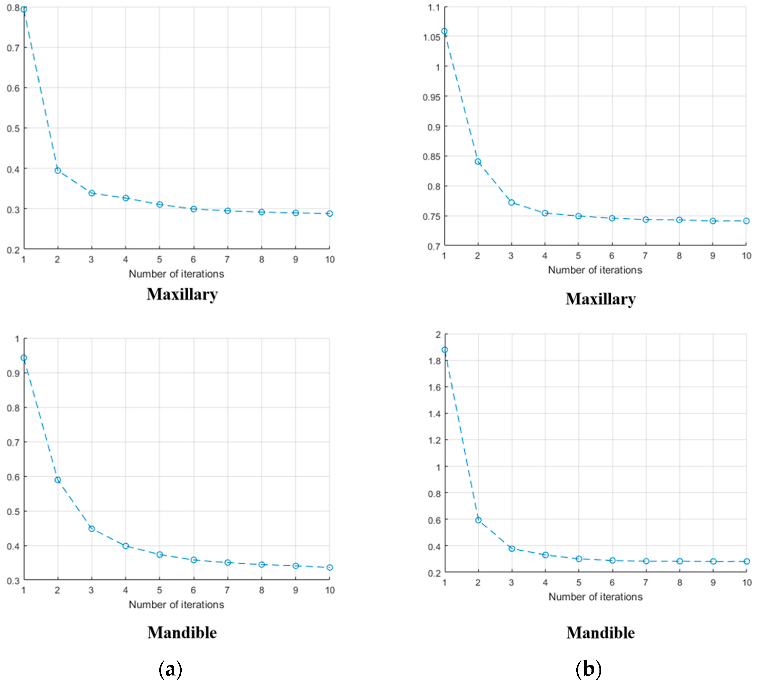
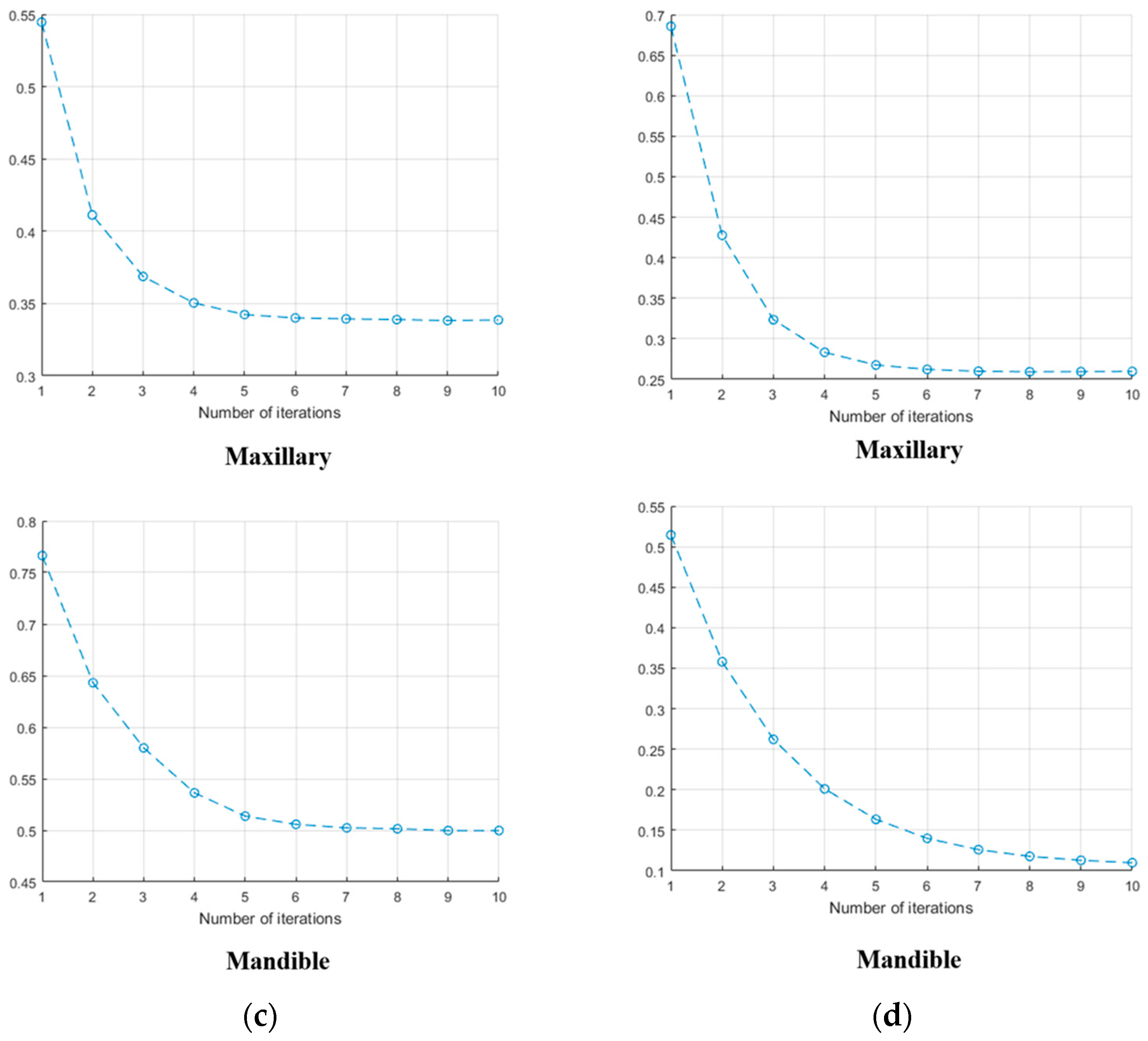
The D value is computed in order to compare the result with the conventional registration result. As mentioned earlier, there is no ground truth for the registration of volume data and surface data. In other words, D = 0 does not exactly correspond to a perfect result. However, it is taken as the ground truth on the basis that the conventional registration is currently used in all dental applications by experts in this field. Maximum tolerance in the registration of volume data and surface data for dental applications ranges from 1.0 mm to 2.0 mm. In most cases, the distance values D between the conventional registration result and the result of the proposed method were less than 2.0 mm. This means that the proposed MICP registration result has fine registration accuracy and can be used for conventional applications without any problem. Also, from the early iterations of MICP, the D values decreased in all test cases. This proves that the surface is moving in the right direction.

While the established registration framework takes more than 20 min to register the volume data and the surface data, the proposed MICP registration takes less than 10 min for all cases because the segmentation process became automatic.

3.2.2. Evaluation of MICP Registration Results by Down Sampling

MICP using full surface data is two times faster than conventional registration and down sampling makes MICP even faster. The MICP registration result using the most down sampled surface data took less than 20 s and varying the D values caused almost no significant difference to this time. If the faster registration of volume data and surface data is needed for some applications, MICP with down sampling is a realistic solution, especially considering that it guarantees fine registration results.

3.2.3. Limitations

In the overall MICP process, segmentation is done automatically but setting the initial condition still needs a human input. Like general ICP, MICP could suffer from poor initial conditions. To determine the maximum effective limits of the initial condition, translations and rotations through x, y, z directions are applied to each data set and used as the initial position of the MICP input data. The D value is used to judge whether the registration works or not with the initial conditions.

To set an initial condition for MICP in real applications, landmarks selected by human input are necessary. In medical image registration, landmark-based registration is widely used instead of total manual registration by picking arbitrary point pairs. Consistency of the landmarks on medical images is about 1.64 mm and this is the initial condition for the registration [42]. This 1.64 mm can be considered directly as the initial condition error. From these initial condition tests, acceptable registration results are obtained with 2 mm differences of translation and rotation.

4. Conclusions

In this paper, modified iterative closest point (MICP), an automatic segmentation method for CBCT volume data and dental scan data is proposed. The proposed registration algorithm is based on a classic local registration algorithm, the iterative closest point (ICP). To find corresponding points for registration of CBCT volume data and dental scan data, previous methods had to extract full surface data from the volume data by segmentation. In the proposed method, the step for finding corresponding points was modified to a dynamic segmentation and the volume data could be directly used as input data. The whole registration process, except for the initial condition setting, is automatic and the registration result of the proposed method differs from conventional registration result by less than 2 mm, which is an acceptable tolerance in the dental CAD/CAM industry. With normal correction, more accurate registration results can be achieved and proper distance values for generating the intensity profile are provided. The registration speed is at least two times faster than the conventional method. With down sampling, MICP works much faster and registration is completed within only 10 s.

References

- Mildenberger, P.; Eichelberg, M.; Martin, E. Introduction to the DICOM standard. Eur. Radiol. 2002, 12, 920–927. [Google Scholar] [CrossRef] [PubMed]
- Gueld, M.O.; Kohnen, M.; Keysers, D.; Schubert, H.; Wein, B.B.; Bredno, J.; Lehmann, T.M. Quality of DICOM header information for image categorization. Med. Imaging 2002, 4685, 280–288. [Google Scholar] [Green Version]
- Mustra, M.; Delac, K.; Grgic, M. Overview of the DICOM standard. In Proceedings of the 2008 50th International Symposium ELMAR, Zadar, Croatia, 10–12 September 2008; Volume 1, pp. 39–44. [Google Scholar]
- Mozzo, P.; Procacci, C.; Tacconi, A.; Tinazzi Martini, P.; Bergamo Andreis, I.A. A new volumetric CT machine for dental imaging based on the cone-beam technique: Preliminary results. Eur. Radiol. 1998, 8, 1558–1564. [Google Scholar] [CrossRef] [PubMed]
- Scarfe, W.C.; Farman, A.G.; Sukovic, P. Clinical applications of cone-beam computed tomography in dental practice. J. Can. Dent. Assoc. 2006, 72, 75–80. [Google Scholar] [CrossRef] [PubMed]
- Scarfe, W.C.; Farman, A.G. What is Cone-Beam CT and How Does it Work? Dent. Clin. N. Am. 2008, 52, 707–730. [Google Scholar] [CrossRef] [PubMed]
- Suomalainen, A.; Vehmas, T.; Kortesniemi, M.; Robinson, S.; Peltola, J. Accuracy of linear measurements using dental cone beam and conventional multislice computed tomography. Dentomaxillofac. Radiol. 2008, 37, 10–17. [Google Scholar] [CrossRef] [PubMed]
- Hiller, J.D.; Lipson, H. STL 2.0: A Proposal for a Universal Multi-Material Additive Manufacturing File Format. In Proceedings of the 20th Solid Freeform Fabrication Symposium (SFF), Austin, TX, USA, 3–5 August 2009; pp. 266–278. [Google Scholar] [CrossRef]
- Morano, R.A.; Ozturk, C.; Conn, R.; Dubin, S.; Zietz, S.; Nissanov, J. Structured light using pseudorandom codes. IEEE Trans. Pattern Anal. Mach. Intell. 1998, 20, 322–327. [Google Scholar] [CrossRef]
- Salvi, J.; Fernandez, S.; Pribanic, T.; Llado, X. A state of the art in structured light patterns for surface profilometry. Pattern Recognit. 2010, 43, 2666–2680. [Google Scholar] [CrossRef]
- Reza Rokn, A.; Hashemi, K.; Akbari, S.; Javad Kharazifard, M.; Barikani, H.; Panjnoosh, M. Accuracy of Linear Measurements Using Cone Beam Computed Tomography in Comparison with Clinical Measurements. J. Dent. 2016, 13, 333. [Google Scholar]
- Patcas, R.; Müller, L.; Ullrich, O.; Peltomäki, T. Accuracy of cone-beam computed tomography at different resolutions assessed on the bony covering of the mandibular anterior teeth. Am. J. Orthod. Dentofac. Orthop. 2012, 141, 41–50. [Google Scholar] [CrossRef] [PubMed]
- Van Assche, N.; Quirynen, M. Tolerance within a surgical guide. Clin. Oral Implant Res. 2010, 21, 455–458. [Google Scholar] [CrossRef] [PubMed]
- Besl, P.; McKay, N. A Method for Registration of 3-D Shapes. IEEE Trans. Pattern Anal. Mach. Intell. 1992. [Google Scholar] [CrossRef]
- Jung, S.; Song, S.; Chang, M.; Park, S. Range image registration based on 2D synthetic images. CAD Comput. Aided Des. 2018, 94, 16–27. [Google Scholar] [CrossRef]
- Gelfand, N.; Mitra, N.J.; Guibas, L.J.; Pottmann, H. Robust global registration. Symp. Geom. Process. 2005, 2, 5. [Google Scholar] [CrossRef]
- Aiger, D.; Mitra, N.J.; Cohen-Or, D. 4-Points Congruent Sets for Robust Pairwise Surface Registration. ACM Trans. Graph. 2008, 27, 1. [Google Scholar] [CrossRef]
- SanthaKumar, R.; Vidhya, S. Three-Dimensional Reconstruction of Cone Beam Computed Tomography Using Splines Interpolation Technique for Dental Application. J. Med Devices 2016, 10, 030927. [Google Scholar] [CrossRef]
- Rumboldt, Z.; Huda, W.; All, J.W. Review of portable CT with assessment of a dedicated head CT scanner. Am. J. Neuroradiol. 2009, 30, 1630–1636. [Google Scholar] [CrossRef] [PubMed]
- Revol, C.; Jourlin, M. A new minimum variance region growing algorithm for image segmentation. Pattern Recognit. Lett. 1997, 18, 249–258. [Google Scholar] [CrossRef]
- Yau, H.T.; Lin, Y.K.; Tsou, L.S.; Lee, C.Y. An adaptive region growing method to segment inferior alveolar nerve canal from 3d medical images for dental implant surgery. Comput. Aided Des. Appl. 2008, 5, 743–752. [Google Scholar] [CrossRef]
- Hosntalab, M.; Aghaeizadeh Zoroofi, R.; Abbaspour Tehrani-Fard, A.; Shirani, G. Segmentation of teeth in CT volumetric dataset by panoramic projection and variational level set. Int. J. Comput. Assist. Radiol. Surg. 2008, 3, 257–265. [Google Scholar] [CrossRef]
- Ji, D.X.; Ong, S.H.; Foong, K.W.C. A level-set based approach for anterior teeth segmentation in cone beam computed tomography images. Comput. Boil. Med. 2014, 50, 116–128. [Google Scholar] [CrossRef] [PubMed]
- Gao, H.; Chae, O. Individual tooth segmentation from CT images using level set method with shape and intensity prior. Pattern Recognit. 2010, 43, 2406–2417. [Google Scholar] [CrossRef]
- Pəvəloiu, I.B.; Vasiləţeanu, A.; Goga, N.; Marin, I.; Ilie, C.; Ungar, A.; Pətraşcu, I. 3D dental reconstruction from CBCT data. In Proceedings of the 2014 International Symposium on Fundamentals of Electrical Engineering, Bucharest, Romania, 28–29 November 2014. [Google Scholar] [CrossRef]
- Mortaheb, P.; Rezaeian, M.; Soltanian-Zadeh, H. Automatic dental CT image segmentation using mean shift algorithm. In Proceedings of the 2013 8th Iranian Conference on Machine Vision and Image Processing (MVIP), Zanjan, Iran, 10–12 September 2013; pp. 121–126. [Google Scholar] [CrossRef]
- Thariat, J.; Ramus, L.; Maingon, P.; Odin, G.; Gregoire, V.; Darcourt, V.; Malandain, G. Dentalmaps: Automatic dental delineation for radiotherapy planning in head-and-neck cancer. Int. J. Radiat. Oncol. Boil. Phys. 2012, 82, 1858–1865. [Google Scholar] [CrossRef] [PubMed]
- Schulze, R.; Heil, U.; Groß, D.; Bruellmann, D.D.; Dranischnikow, E.; Schwanecke, U.; Schoemer, E. Artefacts in CBCT: A review. Dentomaxillofac. Radiol. 2011, 40, 265–273. [Google Scholar] [CrossRef] [PubMed]
- Wang, G.; Snyder, D.L.; O’Sullivan, J.; Vannier, M.W. Iterative Deblurrinf for CT metal artifact reduction. IEEE Trans. Med. Imaging 1996, 15, 657–664. [Google Scholar] [CrossRef] [PubMed]
- Watzke, O.; Kalender, W.A. A pragmatic approach to metal artifact reduction in CT: Merging of metal artifact reduced images. Eur. Radiol. 2004, 14, 849–856. [Google Scholar] [CrossRef] [PubMed]
- Cann, C.E. Quantitative CT for determination of bone mineral density: A review. Radiology 1988, 166, 509–522. [Google Scholar] [CrossRef] [PubMed]
- Norton, M.R.; Gamble, C. Bone classification: An objective scale of bone density using the computerized tomography scan. Clin. Oral Implant Res. 2001, 12, 79–84. [Google Scholar] [CrossRef]
- Turkyilmaz, I.; Ozan, O.; Yilmaz, B.; Ersoy, A.E. Determination of bone quality of 372 implant recipient sites using hounsfield unit from computerized tomography: A clinical study. Clin. Implant Dent. Relat. Res. 2008, 10, 238–244. [Google Scholar] [CrossRef] [PubMed]
- Rafic, M.; Ravindran, P. Evaluation of on-board imager cone beam CT hounsfield units for treatment planning using rigid image registration. J. Cancer Res. Ther. 2015, 11, 690. [Google Scholar] [CrossRef] [PubMed]
- Grimson, W.E.L.; Hildreth, E.C. Comments on “Digital Step Edges from Zero Crossings of Second Directional Derivatives”. IEEE Trans. Pattern Anal. Mach. Intell. 1985, PAMI-7, 121–127. [Google Scholar] [CrossRef]
- Sorkine, O.; Rabinovich, M. Least-Squares Rigid Motion Using SVD. Technical Notes. 2009, pp. 1–6. Available online: http://www.igl.ethz.ch/projects/ARAP/svd_rot.pdf (accessed on 24 February 2009).
- Botsch, M.; Kobbelt, L. An intuitive framework for real-time freeform modeling. ACM Trans. Graph. 2004, 23, 630. [Google Scholar] [CrossRef]
- Kobbelt, L.P.; Bareuther, T.; Seidel, H.P. Multiresolution shape deformations for meshes with dynamic vertex connectivity. Proc. Eurographics 2000 2000, 19, 249–260. [Google Scholar] [CrossRef]
- Gelfand, N.; Ikemoto, L.; Rusinkiewicz, S.; Levoy, M. Geometrically stable sampling for the ICP algorithm. In Proceedings of the Fourth International Conference on 3-D Digital Imaging and Modeling, Banff, AB, Canada, 6–10 October 2003; pp. 260–267. [Google Scholar] [CrossRef]
- Wolf, I.; Vetter, M.; Wegner, I.; Böttger, T.; Nolden, M.; Schöbinger, M.; Meinzer, H.P. The medical imaging interaction toolkit. Med. Image Anal. 2005, 9, 594–604. [Google Scholar] [CrossRef] [PubMed]
- Cignoni, P.; Corsini, M.; Ranzuglia, G. MeshLab: An Open-Source Mesh Processing Tool. In Proceedings of the Eurographics Italian Chapter Conference, Salerno, Italy, 2–4 July 2008; pp. 129–136. [Google Scholar] [CrossRef]
- Schlicher, W.; Nielsen, I.; Huang, J.C.; Maki, K.; Hatcher, D.C.; Miller, A.J. Consistency and precision of landmark identification in three-dimensional cone beam computed tomography scans. Eur. J. Orthod. 2012, 34, 263–275. [Google Scholar] [CrossRef] [PubMed]
Figure 1.
Flow chart: the iterative closest point (ICP)-based method, the established registration method.
Figure 2.
Intensity profile and step edge point.
Figure 3.
Overall procedure of the proposed method.
Figure 4.
Results of normal correction methods for scan data. (a) raw scan data, (b) normal smoothing, (c) remeshing.
Figure 5.
Input data ((a): surface data, (b): volume data). (1) set no.1 (2) set no.2 (3) set no.3 (4) set no.4.
Figure 6.
Conventional registration result. ((a): segmented surface data, (b): maxillary, (c): mandible) (1) set no.1 (2) set no.2 (3) set no.3 (4) set no.
Figure 7.
Registration result of modified iterative closest point (MICP) after normal correction.
Figure 8.
Uniform sampling results. (a) No sampling, (b) uniform sampling (grid size = 1 voxel) (c) uniform sampling (grid size = 5 voxels), (d) uniform sampling (grid size = 10 voxels).