The Progress in Photoacoustic and Laser Ultrasonic Tomographic Imaging for Biomedicine and Industry: A Review

Abstract

The current paper reviews a set of principles and applications of photoacoustic and laser ultrasonic imaging, developed in the Laser Optoacoustic Laboratories of ILIT RAS, NUST MISiS, and ILC MSU. These applications include combined photoacoustic and laser ultrasonic imaging for biological objects, and tomographic laser ultrasonic imaging of solids. Principles, algorithms, resolution of the developed methods, and related problems are discussed. The review is written in context of the current state-of-art of photoacoustic and laser ultrasonic imaging.

1. Introduction

When a laser pulse is absorbed by a medium, instant thermal expansion takes place. This thermal expansion gives rise to an acoustic transient. The amplitude and shape of the transient is determined by the parameters of the laser pulse and properties of the medium. When the laser pulse is short enough (shorter than the transit time of the acoustic wave over the light absorption depth, the so-called condition of stress confinement, and shorter than the characteristic thermal diffusion time—thermal confinement), acoustic transients resemble an absorbed energy distribution. This is the physical basis of the photoacoustic effect that attracted significant attention of scientific and industrial community in the last two decades.

The photoacoustic (PA) or optoacoustic (OA) effect was discovered by Bell in [1] (1880). The first application of this phenomenon was for the measurement of IR absorption in gases [2] (1938). Investigation of the dynamics of excited molecules was performed in [3] (1946). Pulsed lasers open a new area in photoacoustics. Pioneers in this field were Askar’yan, Prokhorov, Chanturiya, and Shipulo [4] (1963). White [5] (1963) proposed the theory of thermal excitation of acoustic transients, due to surface absorption of short electromagnetic bursts. The dependence of the temporal shape of a PA signal on the value of the light absorption coefficient was established in the first experimental investigation of laser–matter interaction using a time-resolved PA method performed by Carome, Clark, and Moeller in [6] (1964). The lack of a theoretical basis, however, did not allow them to obtain quantitative results. The first attempt to give a theoretical explanation of the profile of the PA transient was given by Cleary and Hamrick [7] (1968). The relationship between the spatial distribution of heat sources and the temporal shape of the acoustic signal, excited by a laser pulse, was first theoretically analyzed in [8,9]. The method for measuring the light absorption coefficient from the shape of a PA signal, excited therein, was first suggested and experimentally realized in [10,11], and was later used in [12,13,14,15,16] for biological tissues.

Considerable technological advances in computing, data acquisition, and processing, as well as progress in piezoelectric sensor array manufacturing, lead to rapid development of tomographic techniques employing PA effects. The two most developed and widely applied tomographic imaging modalities are various types of PA imaging (PAI) and laser ultrasonic imaging (LUI).

The main difference between these two modalities is the location of light absorber. In PAI, the light is absorbed inside the investigated object and ultrasound waves carry information about the distribution of the light absorbers. Thus, the contrast in PAI is optical. In the case of LUI, the light is absorbed either in the dedicated external absorbing material (PA generator) or in the surface layer of the investigated object generating probe ultrasonic pulse. This probe pulse is scattered by the acoustic inhomogeneities inside the investigated object, and the scattered waves carry information about the distribution of acoustic inhomogeneities. Thus, the contrast in LUI is acoustic.

Although there are various techniques that are used for conversion of wide-band acoustic waves (mechanical displacement) into electronic signals, including electromagnetic [17] and capacitive transducers [18], in this review, we focus on the two widely used ultrasound detection techniques [18]: piezoelectric transducers [13,19,20] and optical interferometers and deflectors [21,22,23,24]. The non-contact nature of laser generation of ultrasound makes it attractive to develop fully non-contact (all-optical) PAI and laser ultrasonic (LU) evaluation systems employing both optical generation and optical detection of acoustic transients. Although optical sensors can possess ultrawide detection bandwidth [18], surface roughness strongly affects the sensitivity of optical detection, and overall system sensitivity is typically a few orders of magnitude smaller than that of contact wideband ultrasound sensors [24]. Therefore, the main attention is drawn, in this paper, to the piezoelectric detection of acoustic waves. The most sensitive acoustic detectors utilize resonance of physical dimensions and ultrasound waves to be detected. The product of sensitivity and the bandwidth is a constant defined by properties of the detector. Therefore, detection within a narrow frequency band is the most sensitive [25]. However, LU probe pulses, as well as PA ultrasonic transients, have intrinsic wide bandwidth that should be detected if a high spatial resolution is desired.

In the traditional pulse-echo mode of ultrasound (US) imaging, array transducers (linear array, phased array, and curved array) have replaced single element transducers decades back. It helped US imaging devices to become real-time, portable, and handheld. Similarly, the PA community has also adopted array transducers (linear, semicircular, circular, and spherical array) to develop highspeed/real-time PA imaging [26,27,28,29].

Medical imaging is continuously evolving following new medical technologies. The advances in medical imaging tools (X-ray computed tomography (X-ray CT), ultrasound (US), magnetic resonance imaging (MRI), positron emission tomography (PET), and single-photon emission computed tomography, etc.) have led to better diagnosis and patient care [26,30,31,32]. During the last decade, PAI has been evolving rapidly, from the laboratory to preclinical and clinical phases [33,34,35]. PAI is a three-dimensional (3D) hybrid imaging modality that combines the advantages of optical and acoustic imaging. Optical excitation and acoustic detection enable PAI to combine the high contrast available from optical imaging with the spatiotemporal resolution of ultrasound imaging.

Several comprehensive reviews on PAI can be found in the literature [19,22,33,34,36]. There are three types of PAI systems: photoacoustic microscopy (PAM) [34,37,38], photoacoustic endoscopy (PAE) [39], photoacoustic tomography (PAT), or photoacoustic-computed tomography (PACT) [26,33,40].

The interest in PAT is mostly connected with the successful results in tumor diagnostics obtained over the past years [16,22,26,33,34,41]. Time-resolved detection of a PA signal excited by a laser pulse in the investigated medium provides information on the spatial distribution of the optical properties of tissue. Laser pulses may be effectively used to produce acoustic waves in tissue with different optical absorption. Ultrasonic waves can propagate in biological tissue with minimal distortion and deliver diagnostic information to the surface of the tissue, where they may be detected with high temporal resolution by piezoelectric or optical detectors.

Hence, PAT uses the inherent optical contrast of tissue structure. PAT is applicable to almost any problem where the absorption of light occurs [19]. For example, in the task of tumor detection, on the one hand, the contrast of a PA image depends on the large difference in optic absorption between a tumor and healthy tissue. On the other hand, high resolution can be achieved in a PA image. In this case the penetration depth can reach several centimeters, since ultrasonic waves are attenuated much less then light (~1 dB/MHz in the range from 20 kHz to 2 MHz) in soft biological tissues [41].

PAI found applications outside biomedicine. In [42], PAT was proposed as a method for the study of femtosecond filaments in air, and the spatial resolution was studied numerically for this case. In [43], the waveforms calculated numerically were compared with those obtained in experiments. Kerr self-focusing, in the medium, causes a high-power femtosecond laser pulse to overcome the diffraction and collapse, ionizing the medium. Filamentation is a unique optical phenomenon where Kerr self-focusing is balanced with plasma defocusing, so that an elongated plasma column (the core of the filament) is formed. When the plasma recombines, the medium is heated, due to non-radiative de-excitation, and an ultrasonic pulse is generated as in traditional PAI scenarios. The core of the filament is surrounded by laser radiation (the reservoir of the filament), which contains ~90% of the laser pulse energy. In [44], the authors reported a first experimental PAT of a femtosecond filament in water. The position of the filament core was determined with 10 μm accuracy. The authors observed “the halo” around the core in the experimental images and interpreted it as the reservoir of the filament. Thus, PAT has a potential of being a direct high-resolution reservoir imaging technique.

PAT does not replace any current biomedical imaging methods; however, it can complement them. Since PAT combines optics and ultrasound, combining PAT with either optical or ultrasound imaging methods in one complex system is of interest. Since PAT already widely utilizes piezoelectric transducers, PAT systems can be combined with conventional pulse-echo ultrasound. Therefore, such systems can potentially provide not only PA images of endogenous absorbers, such as small blood vessels, but also ultrasound images of mechanical structures, indicating the boundaries of organs. In addition, combined PA and LU imaging can be used to guide invasive procedures, such as needle insertion into blood vessels [45], where the blood vessel is highlighted by PAT, and LUT is used to image the needle. As mentioned, commercial ultrasound detectors have been applied in PAT, such as hand-held arrays, as the PA detector, while optical fibers are used to deliver light [16,46]. Since LUI share similarities with conventional ultrasound, combining PAI and LUI is also of interest.

During the last decade, constant improvements have been made in materials and structures design and control. However, in some problems (e.g., in the field of the reliability), conventional methods (like X-ray computed tomography, conventional ultrasound etc.) are approaching their limits, and the use of the new alternative technologies may be advantageous. LUI can be used for measurements of residual stresses, porosity, local elastic moduli, detection of microscopic internal cracks, and accurate measurements of the surface profile in various materials [47,48,49,50].

LUI systems can employ raster scanning with 1D depth profiling using a single LU transducer, or it can gather scattering information using multiple receivers forming a tomogram. The latter can be called LU tomography (LUT), analogous to PAT. In addition, LUI can be used to reconstruct the distribution of speed of sound in the investigated object with transmission mode time-of-flight measurements [51].

LUT is an acoustic imaging modality that has much in common with conventional ultrasound imaging—the inhomogeneities of compressibility and density in the object reflect and scatter ultrasonic probe pulse. However, the probe pulse is generated in a dedicated light-absorbing material via a photoacoustic effect. While PAT and LUT image different physical properties, they share a common underlying principle of ultrasound generation and reception and, therefore, can share a common laser light source and a common ultrasound detection system, providing complementary information about the object under study. In the following sections, we will discuss the progress in PAT systems, and compare it with LUT with array-based ultrasound transducers.

The separation of the ultrasound generation and detection processes in LUI allows for their separate optimization. The amplitude and the temporal shape of the probe pulse can be optimized for a given task by choosing appropriate laser and material for the PA generator. The piezoelectric transducers can be damped to widen their reception bandwidth (therefore increasing the image quality) at the cost of lower reception sensitivity. However, since the amplitude of the probe pulse can be optimized separately, the overall sensitivity of the system can be maintained.

LUT was applied to the immersion ultrasound profilometry of solid samples [52,53], measurements of internal geometry of solid samples with complex external surface [54], inspection of thick welded joints [55], and evaluation of internal structure of rock samples [56] and biological objects [45,57,58,59,60,61] (often in combination with PAT). These applications will be reviewed, in more detail, below.

2. The Methods of PAI and LUI

2.1. Applications of PAI and LUI—Image Formation Principles

Advantages of the PAI for characterization of optically heterogeneous tissue structures with high spatial resolution were demonstrated over the past several years [14,15,16,62,63]. One of the major merits of PAI is high sensitivity in detecting variations of laser-induced heating. Unique features of PAI found utility in various medical applications, including detection of early cancer [62], monitoring therapeutic effects of lasers in tissues [64,65], and measuring tissue properties and molecular content [26,30,65]. Optimal design and development of PAI and monitoring systems requires, first of all, comprehensive analysis of capabilities and limitations in detection of wide-band ultrasonic transients.

From an image formation standpoint, both conventional ultrasound and PAT can use delay-and-sum type algorithms. However, an important difference between conventional ultrasound and PAT is that ultrasonic systems normally operate in a pulse-echo mode, and it is possible to phase array elements for the radiation whereas, in PAT, the ultrasound sources are inside the investigated object and their radiation pattern is not known in advance. For this reason, the algorithm of image reconstruction is different than in classical ultrasound and, thus, the dependences of resolution and the contrast range of the obtained images differ from the array parameters, as well [66].

The LU method uses sound generation by a laser pulse absorbed in a thin surface layer of the investigated medium, or a dedicated PA generator, the propagation of an ultrasonic pulse in the investigated medium and recording of the passed or scattered ultrasonic signals with high temporal resolution, like conventional ultrasonic method. This trend of object diagnostics is similar to conventional ultrasonic diagnostics and echoscopy [67]. Active research is being conducted to find better materials for PA generators [68]. The advantage of the LU method, compared with other methods, is laser generation of short and intense aperiodic ultrasonic pulses, inaccessible to the usual ultrasonic transducers [69,70]. The method provides efficient excitation in a wide spectral range, from one to tens of megahertz. The short duration of the probing ultrasonic pulse results in an increase in longitudinal spatial resolution, while a reasonable width of the signal band is preserved. The small diameter of the probing beam serves to increase sensitivity; the aperiodic probing pulse almost completely avoids a “dead” zone.

The temporal shape and the amplitude of the ultrasonic pulse depend on the light absorption and thermal conductivity of the medium, the temporal profile of laser pulse intensity, and the density of the absorbed laser energy [70,71]. The pulses have a smooth bipolar profile free from reverberations (Figure 1a). The spectral band of such pulses lies within a wide frequency range, limited only by the spectrum width of the laser pulse (Figure 1b). In contact LUI scenarios, a dedicated PA generator, made of a light-absorbing material, is typically used to generate LU probe pulse [66,70]. In this case, the temporal shape and the amplitude of the pulse are fixed, and can be optimized for the particular task. The surface absorption in the investigated medium can be used, for example, in non-contact LUI applications [55]. The temporal shape and the amplitude of the probe pulse here may depend on a particular point of the sample where the light pulse is absorbed.

2.2. Forward and Inverse Problems of PAT and LUT—Reconstruction Algorithms

2.2.1. Algorithms for PAT

A forward problem for PAT, under the assumption of absorption of short laser pulse and acoustically homogeneous lossless medium, is formulated as a wave equation with initial pressure source:

$$\frac{{\partial }^{2}p}{\partial t^2}-c^2{\nabla }^{2}p=p_0\left(\mathit{r}\right)\frac{d\delta \left(t\right)}{dt},$$

(1)

where $p\left(\mathit{r},t\right)$ is the acoustic pressure field, $c$ is the speed of sound in the medium, $p_0\left(\mathit{r}\right)$ is the initial pressure distribution in the light absorbing material, and $\delta \left(t\right)$ is the Dirac delta function. Note, that $p_0\left(\mathit{r}\right)=\mathsf{\Gamma }\left(\mathit{r}\right)H\left(\mathit{r}\right)$, where $\mathsf{\Gamma }\left(\mathit{r}\right)=\beta c^2/c_p$ is the Gruneisen parameter, $H\left(\mathit{r}\right)$ is the amount of optical energy, absorbed in the medium per unit volume [70], $\beta =-{\rho }^{-1}{\left(\partial \rho /\partial T\right)}_p$ is the volume thermal expansion coefficient, $\rho$ and $T$ are the density and temperature of the medium, $c_p$ is the specific heat capacity at constant pressure.

Solution of Equation (1) is given by

$$p\left(\mathit{r},t\right)=\frac{1}{4\pi c}\frac{\partial }{\partial t}{\int }_{\left|\mathit{r}-\mathit{r}\prime \right|=ct}\frac{p_0\left(\mathit{r}\prime \right)}{\left|\mathit{r}-\mathit{r}\prime \right|}d{S}^{\prime }\left({\mathit{r}}^{\prime },t\right),$$

(2)

where the integral is taken over a surface of a sphere in 3D, and $d{S}^{\prime }$ is the surface element. The inversion of Expression (2) to obtain $p_0\left(\mathit{r}\right)$, using known dependences of pressure on time $p\left({\mathit{r}}_m,t\right)$ in a set of points ${\mathit{r}}_m$, $m=1,\dots ,N$, where $N$ is the number of sensors on the detection surface, is the basis for the majority of the algorithms in PAT. All reconstruction algorithms can be divided into two groups. The first group considers the PA source (the initial pressure distribution) to be continuous, and it includes time-reversal, Fourier-domain, and back-projection algorithms. The second group, which is represented by the model-based algorithms, considers the PA source to be inherently discrete (typically a sum of a finite number of functions with limited support). As there are good reviews on algorithms for PAT (e.g., [72]), they are reviewed here briefly.

Time reversal algorithm. Time reversal is based on the invariance of the wave equation to the substitution $t\to -t$. Let us denote sufficiently large time by $t_0$, so that acoustic pressure in medium volume $V$ decays to $p\left(\mathit{r},t_0\right)=0$. Let us define the reversed pressure wave as

$$p_{tr}\left(\mathit{r},t\right)=p\left(\mathit{r},2t_0-t\right), t_0\le t\le 2t_0.$$

(3)

The inhomogeneous wave equation (Equation (1)) is equivalent to the homogeneous wave equation with initial conditions $p\left(\mathit{r},0\right)=p_0\left(\mathit{r}\right)$ and $\left(\partial p/\partial t\right)\left(\mathit{r},0\right)=0$. The homogeneous wave equation is invariant under transform $t\to -t$, then $p_{tr}\left(\mathit{r},t\right)$ is a solution of homogeneous wave equation with initial conditions $p_{tr}\left(\mathit{r},t_0\right)=p\left(\mathit{r},t_0\right)=0$ and $\left(\partial p_{t\mathit{r}}/\partial t\right)\left(\mathit{r},t_0\right)=- \left(\partial p/\partial t\right)\left(\mathit{r},t_0\right)=0$.

According to Equation (3), time reversal gives the initial distribution of acoustic pressure $p_0\left(\mathit{r}\right)$ at time $t=2t_0$. Measured values are known on the boundary of medium volume $\partial V—$the detection surface $S_0$. Hence, time reversal assumes the solution of system:

$$\{\begin{array}{cc}\frac{{\partial }^2{p}_{tr}}{\partial t^2}-c_0^2\Delta p_{tr}=0& \left(\mathit{r},t\right)\in V\times \left[t_0,2t_0\right]\\ p_{tr}\left(\mathit{r},t_0\right)=\frac{\partial p_{t\mathit{r}}}{\partial t}\left(\mathit{r},t_0\right)=0& \mathit{r}\in V\\ p_{tr}\left(\mathit{r},t\right)=p\left(\mathit{r},2t_0-t\right)& \left(\mathit{r},t\right)\in \partial V\times \left[t_0,2t_0\right]\end{array}.$$

(4)

To find the reconstructed initial pressure distribution $p_0^r\left(\mathit{r}\right)=p_{tr}\left(\mathit{r},2t_0\right)$, the solution can be carried out using, for example, Fourier transform in combination with Green’s function. One of the key advantages of these types of inversion algorithms is that they do not assume the medium to be acoustically homogeneous, and can even be generalized to account for acoustic absorption and dispersion. However, such algorithms are quite computationally expensive, and still cannot be used for real-time imaging.

Fourier transform-based algorithm. Fourier-domain algorithms for PAT [73] are based on the decomposition of the acoustic field. Such algorithms are usually applied when planar detector geometry is used, and the medium is assumed to be acoustically homogeneous. In this case, the acoustic field can be decomposed into the sum of planar monochromatic waves using efficient Fourier transform algorithms. In the cases of spherical and cylindrical detector geometries, the acoustic field has to be decomposed into the sum of spherical or cylindrical waves, respectively, which cannot be done with such high efficiency. They operate using spatial and temporal frequency components $\mathit{k}=\left(k_x,k_y,k_z\right)$ (wave-vector) and $\omega$ (temporal circular frequency) of solution:

$$p\left(\mathit{r},t\right)={\left(2\pi \right)}^{-3}\int P_0\left(\mathit{k}\right)\cos \left(\omega t\right)\exp \left(ı\mathit{k}\cdot \mathit{r}\right)d^3\mathit{k},\omega =c\left|\mathit{k}\right|=c\sqrt{k_x^2+k_y^2+k_z^2},$$

(5)

where $P_0\left(\mathit{k}\right)=\int p_0\left(\mathit{r}\right)\exp \left(-ı\mathit{k}\cdot \mathit{r}\right)d^3\mathit{r}$. The spatial spectrum of the pressure field acquired by the planar detector at the plane $z=0$ is

$$A\left(k_x,k_y,t\right)=\int \int p\left(x,y,z=0,t\right)\exp \left[-ı\left(k_{x}x+k_{y}y\right)\right]dxdy.$$

(6)

The spatial spectrum of the reconstructed initial pressure distribution $P_0^r\left(\mathit{k}\right)$ can be obtained by the inverse spatial Fourier transform of the expression:

$$P_0^r\left[k_x,k_y,k_z=\pm \sqrt{{\left(\omega /c\right)}^2 -k_x^2-k_y^2}\right]=\pm 2\frac{c^2}{\omega }\sqrt{{\left(\omega /c\right)}^2 -k_x^2-k_y^2}{\int }_0^{\infty }A\left(k_x,k_y, t\right)\cos \left(\omega t\right)dt.$$

(7)

Back-projection algorithm. Xu and Wang [74] derived the exact inversion back-projection type formula for the cases of planar, cylindrical, and spherical detector geometries under the assumption of uniform speed of sound in the medium:

$$p_0^r\left(\mathit{r}\right)={\int }_{S_0}\frac{d{\mathsf{\Omega }}_0}{{\mathsf{\Omega }}_0}{\left[2p\left({\mathit{r}}_S,t\right)-2t\frac{\partial p\left({\mathit{r}}_S,t\right)}{\partial t}\right]}_{t=\left|\mathit{r}-{\mathit{r}}_S\right|/c},$$

(8)

where integration is preformed over the detection surface $S_0$, $d{\mathsf{\Omega }}_0$ is the solid angle of the detection surface element $d{S}_0$ at point ${\mathit{r}}_S$, and ${\mathsf{\Omega }}_0$ is the solid angle of the whole surface $S_0$ as seen from point $\mathit{r}$. Expression (8) can be easily interpreted. If there is a point-like PA source at the point, $\mathit{r}$, the travel time $t\left({\mathit{r}}_S\right)$ of the acoustic wave, from this source to the detector at the point ${\mathit{r}}_S$, will be $\left|\mathit{r}-{\mathit{r}}_S\right|/c$. Therefore, for each detector, a “probability sphere” of radius $ct\left({\mathit{r}}_S\right)$ can be constructed, and the PA source will be located at the intersection of all the “probability spheres” for all the detectors. Reconstruction of the amplitude of the PA source requires the quantity in square brackets in (8) to be projected onto the “probability sphere” and all the results for all the detectors to be summed.

Model-based algorithms. Model-based algorithms generally use a discrete representation of (2), with decomposition of initial pressure distribution $p_0\left(\mathit{r}\right)$ into a finite sum of pre-defined basis functions with decomposition coefficients [75,76]. This decomposition usually results in a system of linear equations, which have to be solved to find the vector of decomposition coefficients. For illustration, we follow [75], and take a discrete representation of the integral in (2) in spherical coordinates, expressing the surface element as $d{S}^{\prime }\left({\mathit{r}}^{\prime },t\right)={\left|\mathit{r}-{\mathit{r}}^{\prime }\right|}^2\cos \varphi d\varphi d\theta$

$${\int }_{S^{\prime }\left(\mathit{r},t\right)}\frac{p_0\left(\mathit{r}\prime \right)}{\left|\mathit{r}-\mathit{r}\prime \right|}d{S}^{\prime }\left(\mathit{r}\prime ,t\right)={\int }_{\varphi }{\int }_{\theta }{p}_0\left(\mathit{r}\prime \right)\left|\mathit{r}-\mathit{r}\prime \right|\cos \varphi d\varphi d\theta \approx \Delta \varphi \Delta \theta {\displaystyle \sum }_l{p}_0\left({\mathit{r}}_l^{\prime }\right)\left|\mathit{r}-\mathit{r}\prime \right|\cos {\varphi }_{l,}.$$

(9)

Here, $p_0\left({\mathit{r}}_l^{\prime }\right)$ denotes the values of initial pressure in the points of spatial grid, $\varphi$ and $\theta$ are the spherical coordinates of the surface element $d{S}^{\prime }$, and $\Delta \varphi$ and $\Delta \theta$ are its angular sizes. Combining Equations (2) and (9), discretizing in time, a system of linear equations can be written:

$$p\left({\mathit{r}}_i,t_j\right)\approx {\displaystyle \sum }_{l=1}{a}_l^{ij}{p}_0\left({\mathit{r}}_l^{\prime }\right)\to p=\mathcal{A}{P}_0,$$

(10)

where the second equation is a matrix form of the first equation, $p\left({\mathit{r}}_i,t_j\right)$ is the pressure at time instant $t_j$ recorded by the sensor located at ${\mathit{r}}_i$, $\mathrm{p}=\left\{p\left({\mathit{r}}_i,t_j\right)\right\}$. Here, $\mathcal{A}=\left\{a_l^{ij}\right\}$ is the model matrix, which is defined by the geometry of the setup and the properties of the medium. The vector $P_0$ denotes the initial pressure in grid points, and is to be found, as it gives the distribution of optical absorption. A minimization problem

$$P_0=\arg \underset{\mathcal{P}}{\min }{\Vert p-\mathcal{A}\mathcal{P}\Vert }^2+\mathcal{R},$$

(11)

where $\mathcal{R}$ is a regularization term, has to be solved to find vector $P_0$. The numerical methods, such as LSQR, Moore–Penrose pseudoinverse [76], and others, can be used for this purpose.

Summing up the benefits of different reconstruction algorithms, when a small number of receivers is used ($N\lesssim 100$), the images reconstructed by the time-domain algorithms have less artifacts than those reconstructed by Fourier domain methods. If large number of receivers is used, then the situation is reversed [73]. Fourier domain algorithms are generally fast, due to use of fast Fourier transform. However, they are applicable for real-time imaging only when planar detector geometry is used, and cannot account for non-uniform distribution of speed of sound. Model-based algorithms can be modified to account for different a priori factors and provide more accurate images, but requirements for memory and computational capacities are high. In our studies, we used back-projection algorithm for PAT, as it can be applied to different detector surfaces and can be parallelized for real-time operation. Another advantage is that obtained images are easily interpreted, that enables modification to account for non-uniform speed of sound distribution in a set of important cases.

2.2.2. Algorithms for LUT

In the majority of applications reviewed in the present article, shear waves can be neglected. Therefore, here, we consider a forward problem of ultrasonic tomography in approximation of propagation of longitudinal waves in an infinite medium with no boundaries [77]:

$${\nabla }^{2}p-\frac{1}{c^2}\frac{{\partial }^{2}p}{\partial t^2}={\gamma }_{\kappa }\left(\mathit{r}\right)\frac{1}{c^2}\frac{{\partial }^{2}p}{\partial t^2}+\nabla \cdot \left[{\gamma }_{\rho }\left(\mathit{r}\right)\nabla p\right],$$

(12)

where $\kappa ,\rho$ are constant compressibility and density of the infinite medium, $\tilde{\kappa },\tilde{\rho }$ are actual (inhomogeneous) compressibility and density, ${\gamma }_{\kappa }\left(\mathit{r}\right)=\left(\tilde{\kappa }\left(\mathit{r}\right)-\kappa \right)/\kappa , {\gamma }_{\rho }\left(\mathit{r}\right)=\left(\tilde{\rho }\left(\mathit{r}\right)-\rho \right)/\tilde{\rho }\left(\mathit{r}\right)—$their deviations in a region with an object, $c^{-2}=\rho \kappa$, and $c$ is a speed of sound in the infinite medium. Even in this simplified formulation of the inverse problem, finding reflectivity of the medium is very complicated.

Generally, all ultrasonic algorithms for solution of the inverse problem can be divided into two groups. Algorithms of the first group are based on a ray approach, and the second wave approach to solution of the inverse problem. Wave algorithms provide better resolution; however, they have strong requirements for memory and computational capacity. Therefore, it is more reasonable to use a ray-based approach for real-time imaging applications, which will be shortly reviewed here.

Back-projection. There are few exact inversion formulas derived for ultrasonic tomography, and all of them are derived for soft biological tissues. Most of the inverse problems are solved under Born or Rytov approximations, or iteratively under these approximations. Single scattering covers the majority of regions of interest in nondestructive testing and evaluation (NDT&E) and biological imaging. Norton and Linzer [77] derived one of such solutions for calculation of unknown parameters from backscattering measurements, for the general case of broadband insonification by a spherically diverging probe pulse under the assumption of the first Born approximation. They have shown that, in this case, simple back-projection gives a solution close to exact, under general practical conditions. The back-projection process is an easily interpreted reconstruction procedure, which assumes summing up all the signals recorded by all the sensors, which are known to have been scattered from the specified point.

Synthetic aperture focusing. Many systems for ultrasonic tomography of solids are based on the synthetic aperture focusing technique (SAFT) [78,79,80]. In this technique, an acoustic array of piezoelectric transducers is used in a pulse-echo mode. A single ultrasonic image is obtained by a series of electric pulses. In each “shot”, different time delays are applied to each element of the array in different sequences, to effectively focus the imaging system onto different points of the inspected object. Scattered waves are detected, and electrical signals are used to calculate “one-shot” images by, e.g., back-propagation. The resulting image is obtained by summing up of all “one-shot” images. The multiple “shot” reconstruction leads to a sufficiently long reconstruction process which, however, can be optimized for real-time applications.

A filtered back-projection algorithm can be used in LUT [81]. The PA generator is a plane-parallel plate; therefore, the probe plane wave travels along z-axis towards the acoustic inhomogeneity, located in immersion liquid at the point ${\mathit{r}}_{ij}=\left(x_i,z_j\right)$ of image. The scattered and reflected waves are detected by the $m$-th sensor at the point ${\mathit{r}}_m=\left(x_m,z_m\right)$, $m=1,\dots ,N$. The total travel time is calculated as ${\mathcal{T}}_{ijm}=\left(z+\left|{\mathit{r}}_m-{\mathit{r}}_{ij}\right|\right)/c_0$. The effective amplitude of scatterers is given by the sum over “paraboloids (in 3D) or parabolas (in 2D) of probability”:

$$ϵ\left({\mathit{r}}_{ij}\right)={\displaystyle \sum }_{m=1}^{N}p\left({\mathit{r}}_m,{\mathcal{T}}_{ijm}\right)\cdot \left|{\mathit{r}}_m-{\mathit{r}}_{ij}\right|\cdot \mathcal{D}\left({\mathit{r}}_m,{\mathit{r}}_{ij}\right),$$

(13)

where $ϵ\left({\mathit{r}}_{ij}\right)$—the strength of the scatterer at the point ${\mathit{r}}_{ij}$ of the image, $p\left({\mathit{r}}_m,{\mathcal{T}}_{ijm}\right)—$the amplitude of pressure detected by the $m$-th transducer at time ${\mathcal{T}}_{ijm}$, $\left|{\mathit{r}}_m-{\mathit{r}}_{ij}\right|$ accounts for the $1/r$ attenuation of spherical waves scattered at ${\mathit{r}}_{ij}$, and $\mathcal{D}\left({\mathit{r}}_m,{\mathit{r}}_{ij}\right)$ accounts for directivity pattern of transducers to reduce streak artifacts in the reconstructed image. The back-projection algorithm, in the present form, provides reasonable results, and can be parallelized for real-time operation.

2.3. Spatial Resolution, Sampling, and Limited-View Issues

While the closed-form solution exists for the inverse problem of PA imaging, in practice the measured data is not perfect. The experimental signals contain noise. The sensors have finite bandwidth and aperture, while the reconstruction formulas assume they are point-like. The sensor array contains a finite number of sensors, and the experimental signals contain a finite number of samples, so the problem is discrete, rather than continuous. Finally, the investigated object may not be accessible from all angles, so the sensor array has limited angular aperture (limited view). In addiction, the analytical solutions usually assume lossless acoustically homogeneous medium, which may not be the case in practice. All these imperfections affect the image quality.

The effects of imperfect imaging setup can be quantified using the point-spread function (PSF). PSF is the image of a point source reconstructed by the system. For the perfect system, the PSF is a Dirac delta function. Generally, for a given imaging setup, $PSF\left(\mathit{r}|{\mathit{r}}_0\right)$ functionally depends on the image spatial coordinates $\mathit{r}$, and parametrically depends on the coordinates of the point source ${\mathit{r}}_0$. The imaging system is usually assumed to be linear. In this case, the image of a non-point-like source is a spatial convolution of the source with the PSF. The sizes (e.g., full width at half-maximum, FWHM) of the PSF along three spatial directions—axial, lateral, and elevation—are the spatial resolutions of the system. PSF depends on both the geometrical characteristics of the sensor array and the reconstruction algorithm [82].

Manufacturing of sensor arrays remains a complicated procedure. Therefore, characterization and comparison of sensor array geometries is an important task. In [82,83], the authors propose the sensitivity maps and spatial resolution maps for characterization of the toroidal sensor arrays with limited view and back-projection reconstruction algorithm. Toroidal arrays are promising for real-time 2D imaging with high lateral resolution [84]. Such arrays are curved, both in the image plane (to achieve high lateral resolution) and perpendicular to it (to achieve high elevation resolution). Construction of the sensitivity and spatial resolution maps involves placing a point PA source, calculating the response of all the sensors, accounting for their finite size and bandwidth, reconstructing the image of the source (PSF), and calculating its FWHM in axial and lateral directions (spatial resolutions—dimensions of $PSF\left(\mathit{r}|{\mathit{r}}_0\right)$) and maximum amplitude (sensitivity is $\underset{\mathit{r}}{\max }PSF\left(\mathit{r}|{\mathit{r}}_0\right)$ and depends on ${\mathit{r}}_0$). Figure 2 shows the examples of such maps for cylindrical and spherical sensor arrays.

Having analyzed more than a hundred sensitivity and spatial resolution maps, the authors provided approximate formulas for the FWHM of the sensitivity map along $z$-axis $D$ and the lateral resolution $Lat$ [82]:

$$D^2\left(R\right)=D_F^2+4{\left(R-F\right)}^2{\sin }^2\left[{\left(D_{\infty }^2-D_F^2\right)}^{1/2}/\left(2R\right)\right],$$

$$La{t}^2\left(R\right)=La{t}_F^2+4{\left(R-F\right)}^2{\sin }^2\left[{\left(La{t}_{\infty }^2-La{t}_F^2\right)}^{1/2}/\left(2R\right)\right],$$

where $R$ and $F$ are the radii of curvature of the sensor array in the image plane and perpendicular to it, and $D_F$, $La{t}_F$ are FWHM of the sensitivity region and the lateral resolution for a spherical array ($R=F)$, $D_{\infty }$, $La{t}_{\infty }$—for a cylindrical array ($R\to \infty$). As the radius of curvature increases (sensor array is getting “more cylindrical” and less focused in the image plane) the size of the region with high sensitivity increases, and the lateral resolution worsens. Spherical arrays have the best lateral resolution and the smallest region with high sensitivity. Toroidal geometry of the array can be optimized for a specific task using formulas above.

Earlier the practical limitations for PA imaging were addressed in [85]. Here, we will briefly review the results and try to draw parallels between PA and LU imaging.

In the case of a finite bandwidth of the sensors and full-view reconstruction in ideal medium, the PA PSF is isotropic, spatially independent, and depends on the sensor’s temporal response $h\left(t\right)$: $PSF\left(\mathit{r}|{\mathit{r}}_0\right)=PSF\left(\left|\mathit{r}-{\mathit{r}}_0\right|\right)=-\left(h^{\prime }\left(\left|\mathit{r}-{\mathit{r}}_0\right|/c\right)+h^{\prime }\left(-\left|\mathit{r}-{\mathit{r}}_0\right|/c\right)\right)/\left(4\pi \left|\mathit{r}-{\mathit{r}}_0\right|\right)$. In the case of a finite sensor aperture, the registered signal is a spatial average of the actual ultrasonic field. The PSF is typically spatially dependent and anisotropic. If the sensor’s bandwidth is infinite, the angular size of the PSF (as seen from the center of curvature of the detection surface) is generally equal to the angular aperture of the sensor. The spatial resolution maps show that increasing the radius of curvature in the image plane decreases the lateral resolution. If the detection surface is an infinite plane, the PSF will be spatially independent. The axial resolution in PAI is determined by the bandwidth of the sensors $f_{sens}$, the lateral resolution by the angular size of the sensors in the image plane, and the elevation resolution by the width of the sensors in the elevation direction and focusing.

The axial spatial resolution in LUI seems to be twice as good as the axial resolution in PAI. Let two point-like PA sources (or LU scatterers) be separated by the distance $d$ in the medium with speed-of-sound $c$. The duration $\delta t$ of the temporal response from each source/scatterers is limited by the bandwidth of the sensors (and the duration of the probe pulse in LUI): $\delta t\gtrsim 1/f_{sens}$. The temporal responses from the two point-like PA sources will not overlap when $d/c\gtrsim \delta t\gtrsim 1/f_{sens}$, since the PA pulses travel from the sources to the sensors only once. The temporal responses from the two point-like LU scatterers will not overlap when $2d/c\gtrsim \delta t\gtrsim 1/f_{sens}$ since, first, the LU probe pulse should travel the distance $d$ between the scatterers, and then the reflected pulse should travel the distance $d$ back to the sensor. For the same reason, the LU PSF (the LU image of a point-like acoustic scatterer) is half as thick in the longitudinal direction, in comparison with PA PSF. If, however, the acoustic boundary is highly reflective, the travel-time can be estimated using dedicated time-delay estimation algorithms. In this case, the distance to the boundary can be found with much better accuracy than the size of LU PSF [52,53].

Temporal sampling usually does not pose a problem, provided the sampling frequency of the analog-to-digital converter (ADC) fulfills the Nyquist criterion. Spatial undersampling leads to the increased number of artifacts in the image. The particular shape of the artifacts depends on the reconstruction algorithm. For the back-projection algorithm, the artifacts are streak-shaped. In PAI, the streaks have a spherical (or circular) shape, while in LUI with planar probe pulse, the streaks’ shape is parabolic. In general, the streaks have a shape of lines of constant times-of-flight of the PA or LU acoustic response. The amplitude of the streak artifacts decreases as $1/N$, where $N$ is the number of the sensors, since $N$ streaks are summed coherently in a single point in space where the source is located. Oversampling in the spatial domain (scanning with step-sizes smaller than the sensor’s aperture), as well as oversampling in the time domain, cannot mitigate the blurring if the reconstruction procedure assumes point-like sensors with infinite bandwidth. Hence, sensitivity and spatial resolution maps depend only weakly on the number of sensors [82]. While there are algorithms that may restore the higher frequencies lost during the measurements, they may enhance the high-frequency noise and should be used with care.

Limited view scenarios can be analyzed in the far-field approximation. Let the acoustic field be represented as an infinite sum of plane monochromatic waves (by spatiotemporal Fourier transform). Let the sensor at point $\mathit{r}\left(r,{\theta }_{\mathrm{r}},{\phi }_{\mathrm{r}}\right)=\mathit{n}r$ (where $r,{\theta }_{\mathrm{r}},{\phi }_{\mathrm{r}}$ are the spherical coordinates of the sensor), far away from the source in the origin, detect the plane waves with wave vectors $\mathit{k}=\mathbf{n}\omega /c$. If the PA source is an infinitely thin plane normal to vector $\nu \left(1,\theta ,0\right)$ (Figure 3), then the PA response will be a plane wave with wave vectors $\mathit{k}=\mathbf{\nu }\omega /c$ that can be detected by the sensors with $\mathbf{n}=\mathbf{\nu }$. If the LU reflector is the same infinitely thin plane, and the probe pulse is a plane wave with a wave vector $\mathbf{m}\left(1,\pi ,0\right),$ then the reflected wave will have the wave vectors $\mathit{k}=\mathbf{u}\omega /c$, where $\mathbf{u}\left(1,2\theta ,0\right)$. Therefore, the angular aperture necessary to detect the reflected LU pulse should be twice as large as the angular aperture necessary to detect the PA response. In PAI, the angular aperture of $2\pi$ steradian is sufficient for exact reconstruction, since the PA response in the direction $\left(–\mathsf{\nu }\right)$ can be expressed using the response in the direction $\mathsf{\nu }$. In LU imaging, the acoustic inhomogeneities cannot be reconstructed without full tomographic coverage.

In general, for PA imaging, the “visibility” condition [86] states that the image will be blurred away (“invisible”) at point $P$ on the sharp boundary $L$ of the object, if the normal to $L$ at $P$ does not pass through any receiver (there is no sensor that will detect the corresponding plane wave). In LU imaging, the “visibility” condition is analogous. Non-linear combination of multiple images for different positions of the sensor array [27], or different positions of the point-like sources inside the object [87], can be used to improve image quality. However, these approaches require longer acquisition times.

3. Combining PAI and LUI in Biomedicine

3.1. Hybrid Methods

Rapid evolvement of multimodal (hybrid) techniques is a noticeable trend in biomedical imaging [63,88,89,90,91]. Multimodal systems enable more comprehensive examinations of biological specimens without the need of repositioning them in independent set-ups, thus allowing for a reduction of motion artifacts and higher throughput [91]. By leveraging the strengths of different imaging modalities, hybridization provides a better picture of the tissue anatomy and function as compared to stand-alone modalities [92]. On the one hand, multiple multimodal approaches have been exploited for both preclinical and clinical investigations at the macroscopic level, by combining the different contrast mechanisms available in whole-body imaging modalities, such as X-ray CT, MRI, PET, or SPECT [93,94]. On the other hand, various microscopic methods can also be combined into multimodal devices, in order to examine shallow tissue regions [95,96,97].

Efficient combination of the two modalities (PAT and LUT) may be fundamentally advantageous, since LUT enables easy anatomical navigation and localization of structures, while PAT can provide additional functional information, which translates into better applicability in a clinical setting. As both the modalities are based on ultrasound detection, they can be, in principle, readily combined into a highly complementary hybrid imaging system [98].

In this section, we will review the combination of PAT and LUI diagnostics and their biomedical applications. By “combined systems”, we mean the systems that are capable of co-registering PA and LU pressure signals with the same sensor array. The sensor array provides the same coordinate system for both modalities, and the images can be overlaid [85].

3.2. Combined PA and LU Speed-of-Sound Imaging

LU speed-of-sound (SoS) measurement method found wide applications in material characterization, due to its high accuracy. SoS can be used to determine local elastic moduli, porosity, and residual stresses. Depending on composition of the biological tissue, the SoS can vary between 1350 m/s and 1700 m/s [99]. The quality of PA images reconstructed, without taking into account SoS variations, may be degraded. The short duration and aperiodic waveform of LU probe pulse makes it possible to make accurate transmission mode measurements of the SoS in various media [70], and use the reconstructed SoS map to correct PA images.

In the approximation of geometrical acoustics, the total travel time of a probe pulse along the ray path is

$$\mathcal{T}={\int }_{l\left(\mathit{r}\right)}\frac{dl}{\tilde{c}\left(\mathit{r}\right)},$$

where $\tilde{c}\left(\mathit{r}\right)$ is the inhomogeneous speed of sound, and $l\left(\mathit{r}\right)$ is the ray path. Generally, $l\left(\mathit{r}\right)$ depends on $\tilde{c}\left(\mathit{r}\right)$, and the problem is non-linear. However, if the variations in the speed of sound are small (weakly refractive tissues), the problem can be linearized. If ${\mathcal{T}}_0$ is the travel time and $l\left({\mathrm{r}}_0\right)$ is a straight path in a homogeneous medium with a speed of sound $c$, we get

$$\mathcal{T}={\mathcal{T}}_0+\delta \mathcal{T}\approx {\mathcal{T}}_0+{\int }_{l\left({\mathit{r}}_0\right)}\left(\frac{1}{\tilde{c}\left(\mathit{r}\right)}-\frac{1}{c}\right)dl.$$

Since the integration paths are now straight, we have a form of a classical Radon transform with well-established solution techniques.

Manohar et al. was the first to use a carbon fiber or a horsetail hair placed in the path of laser light as a PA generator, and a US array as a receiver in fan-beam fashioned (Figure 4) SoS imaging [51,99,100,101]. Such a PA generator (which the authors refer to as a “passive element”—PE) acted as a point PA source in the image plane. The laser light was not blocked completely by the PE 250 μm in diameter, and the remaining major part of laser light was used for illumination of the sample and PA imaging. A cross-correlation of the recorded waveforms with the reference waveforms (without a sample) was used to obtain the rough estimate of travel time, and the phase difference $\delta \psi$ at a specific frequency $f$ was used to calculate $\delta \mathcal{T}=\delta \psi /\left(2\pi f\right)$ in [51], because frequency-dependent acoustic attenuation and SoS dispersion in the tissue could cause the pulse shape to degenerate.

The setup was later modified to perform the hybrid “PA + SoS + Acoustic attenuation” imaging [100]. The time-domain travel-time estimation method employed iterative Gauss–Newton optimization for a non-linear problem: $\left[\mathcal{T},\mathrm{A}\right]={\arg }_{\left[\mathsf{\tau },\mathrm{A}\right]}\min {\Vert \mathrm{p}\left(\mathrm{t}\right)-\mathrm{Ah}\left(\mathrm{t}+\mathsf{\tau }\right)\Vert }^2$, where $\mathrm{p}\left(\mathrm{t}\right)$ is the recorded waveform, and $\mathrm{h}\left(\mathrm{t}\right)$ is the signal from the PA generator. The acoustic attenuation was estimated in the frequency domain by minimization accounting for frequency dependence and dispersion. Later, multiple PEs, illuminated all at once by a single laser pulse, were introduced in [101] to speed up data acquisition. Nine horsetail hairs were placed so that signals from individual PEs did not overlap. Although on phantoms, the measurement time was reduced eightfold, the image quality slightly degraded when compared with a single PE. Finally, in [99], the authors employed an iterative TV-regularized reconstruction algorithm that used Eikonal Equation for both SoS and PA imaging: ${\left|\nabla \mathcal{T}\right|}^2= {\tilde{\mathrm{c}}}^{-2}$, where $\nabla \mathcal{T}$ is the gradient of the wavefront. The modified fast marching method was used to calculate the first arrival time, accounting for ray bending according to Snell’s law. The SoS and PA images of a kidney of a mouse embedded in an agar matrix were presented, although SoS map did not detail the inner structure of the organ.

Wurzinger et al. [102] also used multiple PA generators (twenty 1 mm broad stripes of black acrylic paint on a transparent staircase-shaped polymer substrate) for SoS imaging in straight-ray approximation. The authors employed a single free-beam Mach–Zehnder interferometer as a receiver. Pressure waves that crossed the detection laser beam caused the change of the refractive index of water, and corresponding change in the optical path length, which was detected by the interferometer. The setup was later modified to include pulse-echo LU imaging [87] (Figure 4), implemented by the authors earlier [81,103] without SoS imaging.

The setups discussed earlier were designed to acquire the projection data from a 2D slice ($xy$-plane) of an object by rotating the sample. Then, the sample was translated perpendicular to the slice plane (in $z$-direction) to obtain 3D images. Ermilov et al. [104] reported a combined volumetric 3D “PA + SoS” system, where all the projection data was acquired with a single rotation of the sample object. The 150° arc-shaped array, with 64 piezocomposite transducers, was placed vertically (in $xz$-plane), and multiple PA generators were placed diagonally (in the $y=z$ plane) along a straight line. The outputs of 33 optical fibers (600 μm in diameter) were directed at a polymer film painted with black acrylic. For each rotational position of the object, a fiber-optic output of the laser was sequentially aligned, with each of the 33 fiber inputs using a motorized stage and a ball-lens projection system. The full SoS scanning time was 1.5 h. The SoS maps were reconstructed in straight-ray approximation with TV regularization. 3D multi-wavelength PA images of a nude mouse in vivo, and combined 3D “PA + SoS” images of phantoms, were presented.

3.3. Combined PA and LU Pulse-Echo Imaging

PA imaging can be combined with pulse-echo ultrasound imaging. PA imaging has high contrast and can provide spectroscopic information, while ultrasound can provide morphological and anatomical information about the surrounding tissues and structures. Thus, numerous systems combining PA imaging with conventional B-mode ultrasound (US) imaging were proposed (e.g., [84,105,106,107,108,109,110,111,112,113]) and some integrated PAUS systems are commercially available (e.g., Fujifilm VisualSonics Vevo LAZR or Seno Medical Instruments Imagio). LUI may be advantageous, since it may use the same laser pulse to generate the probe pulse and the bandwidth of the probe pulse may be wider (from 1 to 10 MHz). The ultrasound transducers can also be optimized for wideband reception and better acoustic coupling, since they are not used for ultrasound generation.

Simonova et al. [41] were, to the best to our knowledge, the first to manufacture a combined “PA + LU” system. The system contained a planar array of sixteen 1 mm-wide broadband (1.6–9 MHz) polyvinylidene fluoride (PVDF) piezoelectric transducers glued to the plane-parallel black polymer film (100 μm thick) as a PA generator and poly (methyl methacrylate) (PMMA) cylindrical focusing acoustic lens (Figure 5) for 2D “PA + LU” imaging. The piezoelectric elements were damped, and detected the full PA generation bandwidth. Later [45], the system was equipped with a real-time field-programmable gate array (FPGA)-based data acquisition system, and used for medical needle guidance studies. PA imaging was used to locate the polymeric blood vessel model filled with a diluted Indian ink solution, and LU imaging was used to track the position of the needle tip inside the vessel. The setup was proposed to prevent piercing blood vessels through. In this scenario, both the blood vessel and the needle acted as PA sources, so LUI helped to determine the needle tip position inside the vessel more accurately. The achieved frame rate was 10 Hz. The acceptance angle of the needle was not studied in [45], but it was noted that wideband LU probe pulse reverberates inside the needle, which could be used to identify the needle.

It is worth noting that combined “PA + US” systems, proposed for needle guidance earlier [114,115], used PAI differently. There, the needle acted as a cylindrical PA source, and the PA image showed the position of the needle relative to the US array and the injected absorptive agent, while the US image provided anatomical landmarks. In this imaging scenario, the PA imaging helped to enhance the contrast of US images of the needle and effectively double the acceptance angle $\mathsf{\vartheta }$ between the needle and the linear US array. In the purely US needle guidance scenarios, the needle acts as an ultrasonic reflector, since it has an order of magnitude higher acoustic impedance than the surrounding tissue. However, the acoustic wave reflected from the needle travels at the $2\mathsf{\vartheta }$ angle to the linear array. In PAI of the needle, the wave generated by the needle travels along the normal of the needle, so the angle of incidence on the array is equal to $\mathsf{\vartheta }$. If the angle of incidence exceeds the angular size of the main lobe of the piezoelectric sensor, the needle becomes “invisible”. It could also be said that the effective doubling of the acceptance angle occurs because the angular aperture necessary to detect the reflected LU pulse should be twice as large as the angular aperture necessary to detect the PA response. While, in [115], the achieved frame rate (10 Hz) was limited by the repetition rate of the high-power laser and, in [41], the authors used a high repetition rate (~1 kHz) laser with relatively low pulse energy (~2 mJ), and integrated it with a real-time clinical ultrasound scanner. The narrow laser beam was scanned over the imaging area using a rotating galvo-mirror, and the 256-element linear US array was used for both modalities. The combined PA/US imaging system achieved 30 frames (2.8 × 2.8 cm) per second.

Another approach to needle guidance is integrating the PA generator and ultrasound sensor into the needle tip [116,117,118]. In [117], the needle contained three fibers. The authors used a Fabry–Pérot cavity (two dielectric mirror coatings with an epoxy spacer in between) manufactured on the end face of the fiber as a receiver, a composite coating (polydimethylsiloxane with integrated multiwalled carbon nanotubes) on the end face of another fiber. The third fiber was supposed to be used for PA illumination; it was not used in [117], but was used in [116]. The needle tip tracking was implemented in [116]. The linear US array, at the tissue surface, transmitted acoustic pulses which were received by the fiber-optic sensor in the needle tip. The accuracy was better than 1 mm in both axial and lateral dimensions. One of the main challenges was crosstalk, since the generator and the receiver were situated at a very close proximity inside the needle. In [118], a custom needle with a metallic septum between the two fibers for acoustic isolation was used.

The combined “PA + LU + SoS” setup, by Wurzinder et al. [57], employed optical detection of ultrasonic waves. This work expanded on the authors’ earlier setup [81,103] that combined PA and pulse-echo LU imaging. The same laser pulse was used for illuminating the object in PA mode, the PEs in SoS mode, and the PA generator in LU mode. The same laser beam was used for ultrasound detection, making the setup all-optical. The PA signals from the object, LU probe pulse, LU echo signals, and LU transmission signals all arrived at different times, allowing their separation. This non-overlapping condition limited the maximum diameter of the sample object. Focusing into the 2D plane was achieved by a concave cylindrical acoustic mirror coated with 100 nm thick Cr-layer, used as a PA generator for pulse-echo LU imaging. The spatial resolution of the optical detector is limited by the beam waist (~35 μm). The overlaid “PA + LU” images of transparent zebrafish embedded in gelatin and “PA + LU + SoS” images of phantoms were presented.

Fehm et al. [58] reported a hand-held combined real-time 3D “PA + LU” imaging system. The authors earlier [43] presented a custom-made sensor array (256 3 × 3 mm piezocomposite elements) with a shape of a spherical cap covering an angle of 90°. The curvature radius was 40 mm. On the axis of the array, the fiber bundle for illumination was embedded. On the same axis a carbon microsphere (PE) ~400 μm in diameter was placed embedded in agar ~1.5 cm from the focal point. Thus, the illumination was not blocked completely, and both the object and the microsphere were illuminated simultaneously. Back-projection algorithm, implemented on a GPU, was used for real-time PA and LU image reconstruction (10 volumetric frames per second). It was noted that the emitted spectrum was significantly broader than the detection bandwidth of the piezocomposite transducers, and a band-pass filter from 2 MHz to 4 MHz was applied. Authors presented the “PA + LU” images of phantoms and a human finger. The achieved spatial resolution in LU mode was ~500 μm, due to the size of the PE, and a smaller PE could not be used due to image contrast deterioration. Later, in [119], the authors presented a hemispherical array with 510 broadband piezocomposite elements, 1 mm in diameter and with a curvature radius of 15 mm. The system was capable of 100 volumetric PA images per second. LU imaging mode was not implemented.

Completely non-contact “PA + LU” imaging setups [59,60,61] should also be mentioned. The LU probe pulse can be generated in the subsurface layer of the biological tissue [59]. Alternatively, a dedicated absorbing film or tape can be applied to the surface of the tissue [60,61].

4. Laser-Ultrasonic Imaging of Solid Bodies

In recent years, imaging of solids has drawn much research attention [55,120]. While non-destructive testing and evaluation of objects with complex shapes have numerous practical applications, they pose a significant challenge. For a wide range of industrial control applications, the problem of surface profile measurements is very important [121,122]. X-ray-computed tomography, used often to solve this task, requires access to the object from all sides, and has low spatial resolution for visualization of small internal cracks. These features limit the applicability of X-ray tomography, and can be partially overcome by ultrasonic methods [52] that have improved rapidly these last years.

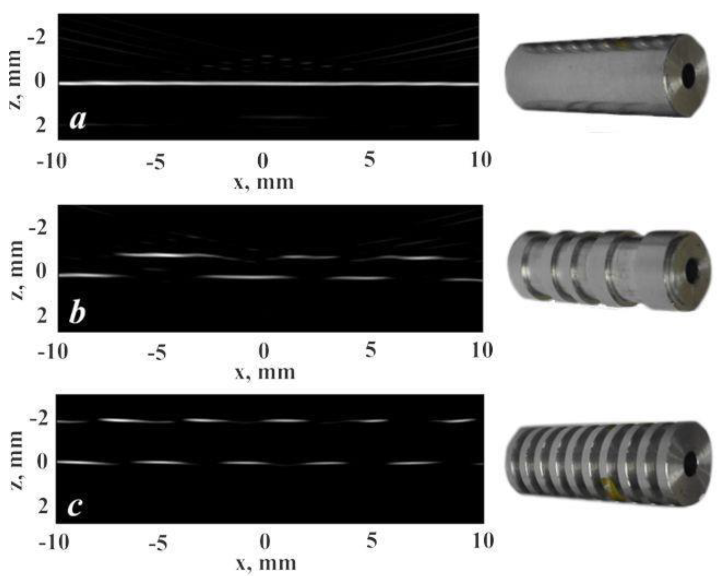
4.1. LU Profilometry of Solids

The LU modality of the combined PA and LU imaging system developed by Simonova et al. [45] was applied to the profile measurement of solid objects [52]. There are several common types of profilometers, such as contact stylus profilers, or non-contact optical profilers. However, such systems are not applicable for inspection of immersed or contaminated objects. For measurement of such objects (e.g., pipes, oil tanks, objects in cooling liquids, underwater works), the developed setup for LU profilometry provides high acoustic resolution in real time: in the longitudinal direction (along the probe pulse beam) up to 20–40 $\mathsf{\mu }\mathrm{m}$; and in transverse, up to 150–250 $\mathsf{\mu }\mathrm{m}$ (along the direction perpendicular to the probe beam).

2D LU images of solid samples are obtained using the back-projection algorithm (Equation (13)) described above. In Figure 6, the negative part of the images is truncated, while white boundaries denote reflections from the sample profile. Images are reconstructed under the assumption of uniform speed of sound in the whole domain of measurements. Hence, only the positions of water–solid interfaces are correctly displayed, and all the positions of the scatterers inside the object (the internal structure) are distorted.

Let the immersion liquid (water) have speed of sound $c_0$ and density ${\rho }_0$, and let the sample have speed of sound $c_1$ and density ${\rho }_1$. As the acoustic impedance of water $Z_0={\rho }_0{c}_0$ is significantly lower than that of material of the sample (duralumin) $Z_1={\rho }_1{c}_1$, the reflection coefficient of the acoustic waves is positive, and takes the greatest value on the water–solid interface. Hence, the position of sample profile on the tomogram is defined by the first local maximum of the obtained tomograms. A set of such local maxima forms the LU image of the surface profile (Figure 7a). A Hough transform and linear least squares method are applied to the set of profile points, to find linear regions. This procedure enables calculation of the deviation of the measured sample profile from the model. Comparison of images, obtained by LU measurements and X-ray imaging has shown good agreement of the results. The discrepancy of the results was within 20–30 $\mathsf{\mu }\mathrm{m}$ in the longitudinal direction, and 150–250 $\mathsf{\mu }\mathrm{m}$ in the transverse direction. The properties of such resolution are connected to the fundamental properties of all ultrasonic measurements: in the direction along the acoustic beam path, the resolution is significantly higher than in the perpendicular direction.

Reconstruction of the 3D surface profiles (Figure 7b,f) was performed using step-by-step 2D imaging with sample rotation and subsequent composition of the profile lines into the surface. Figure 7e shows 3D image of the same object as in Figure 7c, but with a damaged surface. The diameters of parts, measured by X-ray tomography and LU measurements, showed agreement within 100–150 $\mathsf{\mu }\mathrm{m}$. This discrepancy is caused mainly by misalignment of the rotational axis and the object’s axis of symmetry.

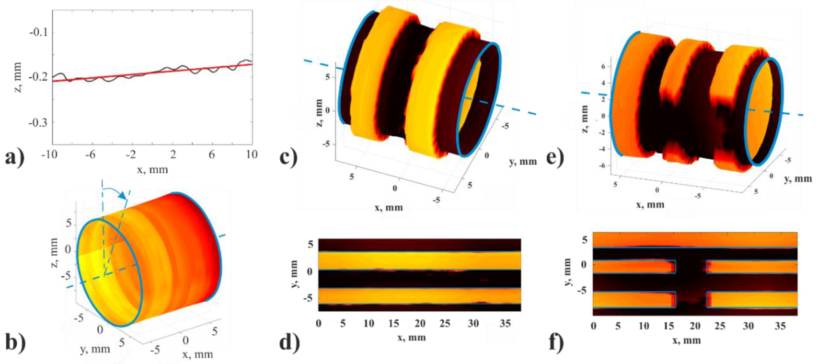
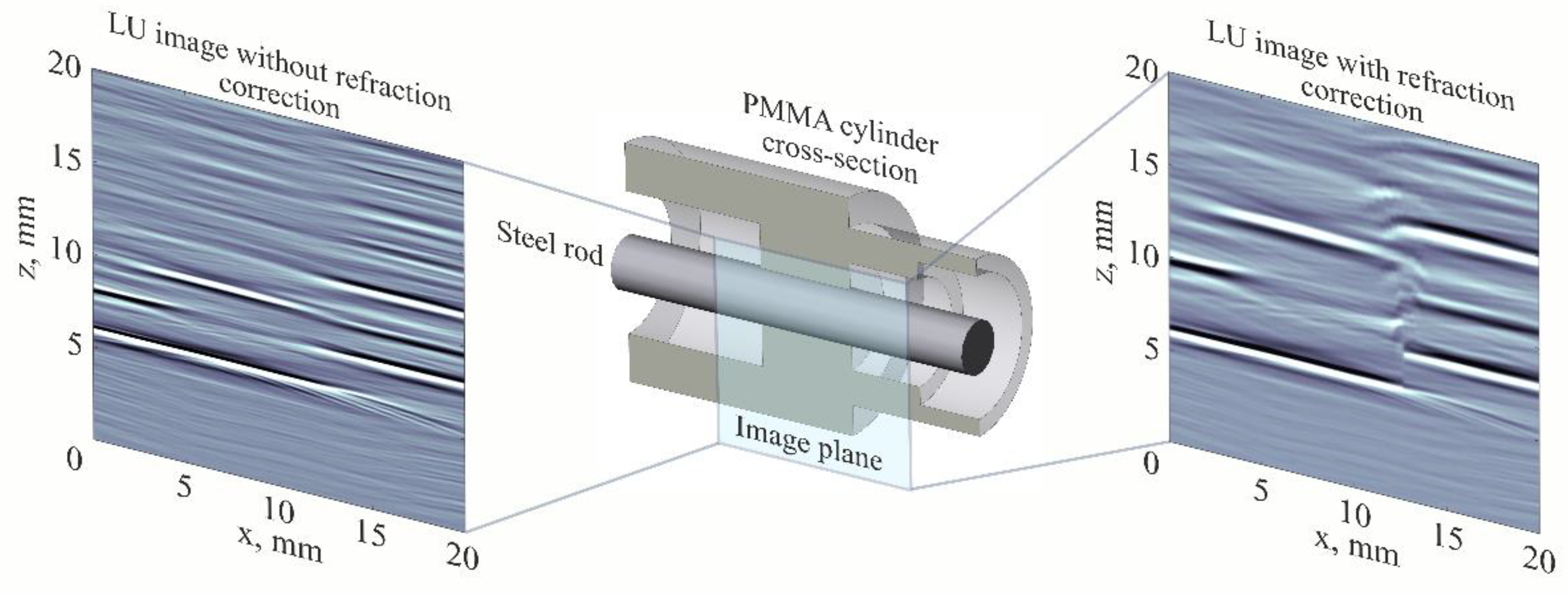
4.2. LU Measurements of Geometry of Solids with Complex Surface

The ability to segment the profile in LU images allows for the internal part of samples with complex surface to be imaged correctly [54]. In this way, such limitations of X-ray tomography for solids, as low sensitivity and requirement of access to inspected object from all sides, can be overcome for a set of applications.

The refraction of ultrasonic waves that occurs at the water–solid interface can be taken into account by a two-step algorithm based on a heuristic ray tracing technique demonstrated in [54], for solids with piecewise-linear surface profiles. First, the profile is obtained in the form of the equations of linear segments analogous to the LU profilometry (Section 4.1). Second, a part of image corresponding to the internal part of the sample is recalculated, accounting for the changes in the time-of-flight and amplitude, introduced by refraction on the solid–water interface.

The propagation of acoustic waves in the approximation of geometrical acoustics is shown in Figure 8. The total path of the acoustic ray can be divided into forward and backward paths. Then, the total travel time is

$${\mathcal{T}}_{ijm}={\mathcal{T}}_{ij}^{forw}+{\mathcal{T}}_{ijm}^{back},$$

(14)

where ${\mathcal{T}}_{ij}^{forw}, {\mathcal{T}}_{ijm}^{back}$ are the travel times on forward (from PA generator to $\left(i,j\right)$ pixel of image) and backward (from $\left(i,j\right)$ pixel of image to $m$-th detector) paths, correspondingly. The positions of ray entry $\left(x_e,z_e\right)$ and exit $\left(x_o,z_o\right)$ from sample should be calculated to determine these times, under the assumption of homogeneous speed of sound in both media. The coordinates of the entry point are calculated from the Snell’s law, and the equations of line profiles know from the LU profilometry. In the first Born approximation, the inhomogeneity, located in the point $\left(x_i,z_j\right)$, scatters waves in all directions, and the coordinates of the exit point $\left(x_o,z_o\right)$ are calculated following the Fermat’s principle of least time for ${\mathcal{T}}_{ijm}^{back}$, which is achieved at the profile lines:

$$\{\begin{array}{c}{\mathcal{T}}_{ijm}^{back}\left(x_o,z_o\right)=\frac{1}{c_0}\sqrt{{\left(z_o-z_m\right)}^2+{\left(x_o-x_m\right)}^2}+\frac{1}{c_1}\sqrt{{\left(z_o-z_i\right)}^2+{\left(x_o-x_j\right)}^2}\to \min ,\\ z_o=k_s{x}_o+b_s,\end{array}$$

(15)

where $k_s$ and $b_s$ are the coefficients of the $s$-th line of surface profile. The gradient descent method can be applied to solve this minimization problem.

The expression for the recalculated part of the image corresponding to the internal part of the object can be obtained from Equation (13), with modified times-of-flight and amplitudes:

$${ϵ}^{\prime }\left({\mathit{r}}_{ij}\right)={\displaystyle \sum }_{m=1}^{N}p\left({\mathit{r}}_m,{\mathcal{T}}_{ijm}\right)\cdot \mathcal{D}\left({\mathit{r}}_m,{\mathit{r}}_{ij}\right)\cdot W_{ijk}^{ol}{W}_{ijm}^{el},$$

(16)

where $W_{ijk}^{ol},W_{ijm}^{el}$ are the coefficients used to account for the partial transmission and mode-conversion (longitudinal waves in water into transverse waves in the solid sample) on the forward and backward paths, correspondingly. They are evaluated standard formulas from [123].

The sample (Figure 9a) is a PMMA cylinder with complex internal and external generatrices. In the image obtained after the first step of the algorithm (Figure 9b), the internal part of the sample appears “squeezed” vertically. The corrected image (Figure 9c) shows the real sample dimensions. The comparison of the results of measurement by LUI and standard gauge measurements showed agreement of the results within $100 \mathsf{\mu }\mathrm{m}$ in the longitudinal (along z-axis) direction in PMMA, and $200-300 \mathsf{\mu }\mathrm{m}$ in the transverse direction (along x-axis).

5. Conclusions

The research in the fields of PAI and non-contact LUI is highly active. The interest in PAI is primarily biomedical (cancer diagnostics, small animal imaging etc.) while the interest in non-contact LUI is primarily industrial (early-stage inspection, additive technologies, inspection in harsh environments etc.). The promising results of these techniques draw considerable attention from the scientific and industrial community. However, today, there is a lack of review papers about the contact LU method. Thus, the purpose of this review is to put a spotlight on the contact LUI and its combinations with PAI, and discuss the algorithms, experimental setups, applications, etc.

The research in the Laser Optoacoustic Laboratories of ILIT, NUST MISiS, and ILC MSU is primarily concerned with tomographic diagnostics of objects that are of interest for biomedicine and industry. Nowadays, tomographic imaging is a hot topic, since it can provide detailed information about the internal structure, reliability, and safety. One of the important advantages of PAI and LUI is mobility, high speed of operation (up to real time), and moderate cost in comparison with other well-established imaging modalities (like MRI, X-ray CT, neutron imaging etc.). Besides, PAI and LUI are usually safer for humans, since the necessary power of laser radiation can comply with safety standards in PAI, or can be confined inside the setup in contact LUI. Perhaps, PAI and LUI cannot replace the well-established and highly developed techniques completely, however, they can provide valuable complementary information about the object and can be integrated in the existing systems.

In this paper, we observe methods and algorithms of PAI and LUI imaging first, then we discuss the combined PAI and LUI systems and their biomedical applications in more detail and, finally, we focus on the immersion LU profilometry and tomography as an example of a possible industrial application of LUI.

References

1. Bell, A.G. On the production and reproduction of sound by light. Am. J. Sci. 1880, 3, 305–324. [Google Scholar] [CrossRef]
2. Veingerov, M.L. New method of gas analysis based on optoacoustic Tyndall-Röntgen phenomena. Dokl. Akad. Nauk SSSR 1938, 19, 687–688. [Google Scholar]
3. Gorelik, G.S. On a possible method of studying the energy exchange time between the different degrees of freedom of molecules in a gas. Dokl. Akad. Nauk SSSR 1946, 54, 779. [Google Scholar]
4. Askar’yan, G.A.; Prokhorov, A.M.; Chanturiya, G.F.; Shipulo, G.P. The effects of a laser beam in a liquid. Sov. Phys. JETP 1963, 17, 1463–1465. [Google Scholar]
5. White, R.M. Generation of elastic waves by transient surface heating. J. Appl. Phys. 1963, 34, 3559–3567. [Google Scholar] [CrossRef]
6. Carome, E.F.; Clark, N.A.; Moeller, C.E. Generation of acoustic signals in liquids by ruby laser-induced thermal stress transient. Appl. Phys. Lett. 1964, 4, 95–97. [Google Scholar] [CrossRef]
7. Cleary, S.F.; Hamrick, P.E. The generation of elastic plane wave by linear thermal transient. Va. J. Sci. 1968, 19, 228–231. [Google Scholar]
8. Burmistrova, L.V.; Karabutov, A.A.; Portnyagin, A.I.; Rudenko, O.V.; Cherepetskaya, E.B. The method of transfer functions in problems of thermooptical sound generation. Sov. Phys. Acoust. 1978, 24, 655–663. [Google Scholar]
9. Karabutov, A.A.; Rudenko, O.V.; Cherepetskaya, E.B. To the theory of thermooptical generation of non-stationary acoustic fields. Sov. Phys. Acoust. 1979, 25, 383–394. [Google Scholar]
10. Karabutov, A.A.; Portnyagin, A.I.; Rudenko, O.V.; Cherepetskaya, E.B. Nonlinear transformation of thermooptically excited acoustic pulses. Sov. Phys. JETP Lett. 1979, 5, 369–373. [Google Scholar]
11. Karabutov, A.A.; Omel’chuk, N.N.; Rudenko, O.V.; Chupryna, V.A. Quantitative study of the nonlinear transformation of sound pulses in liquid under thermooptical excitation. Moscow Univ. Bull. Ser. 1985, 40, 72–77. [Google Scholar]
12. Cross, F.W.; Al-Dhahir, R.K.; Dyer, P.E.; MacRobert, A.J. Time-resolved photoacoustic studies of vascular tissue ablation at three laser wavelengths. Appl. Phys. Lett. 1987, 50, 1019–1021. [Google Scholar] [CrossRef]
13. Oraevsky, A.A.; Esenaliev, R.O.; Jacques, S.L.; Tittel, F.K. Laser optoacoustic tomography for medical diagnostics principles. Proc. SPIE 1996, 2676, 22–32. [Google Scholar] [CrossRef]
14. Brochu, F.; Brunker, J.; Joseph, J.; Tomaszewski, M.R.; Morscher, S.; Bohndiek, S.E. Towards quantitative evaluation of tissue absorption coefficients using light fluence correction in optoacoustic tomography. IEEE Trans. Med. Imaging 2017, 36, 322–331. [Google Scholar] [CrossRef] [PubMed]
15. Hupple, C.W.; Morscher, S.; Burton, N.C.; Pagel, M.D.; McNally, L.R.; Cárdenas-Rodríguez, J. A light-fluence-independent method for the quantitative analysis of dynamic contrast-enhanced multispectral optoacoustic tomography (DCE MSOT). Photoacoustics 2018, 10, 54–64. [Google Scholar] [CrossRef] [PubMed]
16. Becker, A.; Masthoff, M.; Claussen, J. Multispectral optoacoustic tomography of the human breast: Characterisation of healthy tissue and malignant lesions using a hybrid ultrasound-optoacoustic approach. Eur. Radiol. 2018, 28, 602–609. [Google Scholar] [CrossRef] [PubMed]
17. Murfin, A.S.; Soden, R.A.J.; Hatrick, D.; Dewhurst, R.J. Laser-ultrasound detection systems: A comparative study with Rayleigh waves. Meas. Sci. Technol. 2000, 11, 1208–1219. [Google Scholar] [CrossRef]
18. Lutzweiler, C.; Razansky, D. Optoacoustic imaging and tomography: Reconstruction approaches and outstanding challenges in image performance and quantification. Sensors 2013, 13, 7345–7384. [Google Scholar] [CrossRef] [PubMed]
19. Karabutov, A.A.; Podymova, N.B.; Letokhov, V.S. Time-resolved laser optoacoustic tomography of inhomogeneous media. Appl. Phys. B 1996, 63, 545–563. [Google Scholar] [CrossRef]
20. Oraevsky, A.A.; Esenaliev, R.O.; Jacques, S.L.; Thomsen, S.; Tittel, F.K. Lateral and z-axial resolution in laser optoacoustic imaging with ultrasonic transducers. Proc. SPIE 1995, 2389, 198–208. [Google Scholar] [CrossRef]
21. Dewhurst, R.J.; Shan, Q. Optical remote measurement of ultrasound. Meas. Sci. Technol. 1999, 10, R139. [Google Scholar] [CrossRef]
22. Beard, P. Biomedical photoacoustic imaging. Interface Focus 2011, 1, 602–631. [Google Scholar] [CrossRef] [PubMed] [Green Version]
23. Esenaliev, R.O.; Karabutov, A.A.; Oraevsky, A.A. Sensitivity of laser opto-acoustic imaging in detection of small deeply embedded tumors. IEEE J. Sel. Top. Quant. Electr. 1999, 5, 981–988. [Google Scholar] [CrossRef]
24. Pelivanov, I.; Buma, T.; Xia, J.; Wei, C.-W.; O’Donnell, M. A new fiber-optic non-contact compact laser-ultrasound scanner for fast non-destructive testing and evaluation of aircraft composites. J. Appl. Phys. 2014, 115, 113105. [Google Scholar] [CrossRef] [PubMed] [Green Version]
25. Oraevsky, A.; Karabutov, A. Ultimate sensitivity of time-resolved opto-acoustic detection. Proc. SPIE 2000, 3916, 1–12. [Google Scholar]
26. Upputuri, P.K.; Pramanik, M. Recent advances toward preclinical and clinical translation of photoacoustic tomography: A review. J. Biomed. Opt. 2016, 22, 041006. [Google Scholar] [CrossRef] [PubMed]
27. Li, G.; Li, L.; Zhu, L.; Xia, J.; Wang, L.V. Multiview Hilbert transformation for full-view photoacoustic computed tomography using a linear array. J. Biomed. Opt. 2015, 20, 066010. [Google Scholar] [CrossRef] [PubMed] [Green Version]
28. Dean-Ben, X.L.; Razansky, D. Portable spherical array probe for volumetric real-time optoacoustic imaging at centimeter-scale depths. Opt. Express 2013, 21, 28062–28071. [Google Scholar] [CrossRef] [PubMed]
29. Esenaliev, R.; Petrov, I.; Petrov, Y.; Guptarak, J.; Boone, D.R.; Mocciaro, E.; Weisz, H.; Parsley, M.A.; Sell, S.L.; Hellmich, H.; et al. Nano-pulsed laser therapy is neuroprotective in a rat model of blast-induced neurotrauma. J. Neurotrauma 2018, 35, 1510–1522. [Google Scholar] [CrossRef] [PubMed]
30. Xu, M.; Wang, L.V. Time-domain reconstruction for thermoacoustic tomography in a spherical geometry. IEEE Trans. Med. Imaging 2002, 21, 814–822. [Google Scholar] [PubMed] [Green Version]
31. Lu, G.; Fei, B. Medical hyperspectral imaging: A review. J. Biomed. Opt. 2014, 19, 010901. [Google Scholar] [CrossRef] [PubMed]
32. Aldrich, M.B.; Marshall, M.V.; Sevick-Muraca, E.M.; Lanza, G.; Kotyk, J.; Culver, J.; Wang, L.V.; Uddin, J.; Crews, B.C.; Marnett, L.J.; et al. Seeing it through: Translational validation of new medical imaging modalities. Biomed. Opt. Express 2012, 3, 764–776. [Google Scholar] [CrossRef] [PubMed]
33. Zhou, Y.; Yao, J.; Wang, L.V. Tutorial on photoacoustic tomography. J. Biomed. Opt. 2016, 21, 061007. [Google Scholar] [CrossRef] [PubMed] [Green Version]
34. Wang, L.V.; Gao, L. Photoacoustic microscopy and computed tomography: From bench to bedside. Annu. Rev. Biomed. Eng. 2014, 16, 155–185. [Google Scholar] [CrossRef] [PubMed]
35. Brunker, J.; Yao, J.; Laufer, J.; Bohndiek, S.E. Photoacoustic imaging using genetically encoded reporters: A review. J. Biomed. Opt. 2017, 22, 070901. [Google Scholar] [CrossRef] [PubMed]
36. Oraevsky, A.A.; Andreev, V.G.; Karabutov, A.A.; Esenaliev, R.O. Two-dimensional optoacoustic tomography: Array transducers and image reconstruction algorithm. Proc. SPIE 1999, 3601, 256–267. [Google Scholar]
37. Chen, S.-L.; Guo, L.J.; Wang, X. All-optical photoacoustic microscopy. Photoacoustics 2015, 3, 143–150. [Google Scholar] [CrossRef]
38. Zhang, H.F.; Maslov, K.; Stoica, G.; Wang, L.V. Functional photoacoustic microscopy for high resolution and noninvasive in vivo imaging. Nat. Biotechnol. 2006, 24, 848–851. [Google Scholar] [CrossRef] [PubMed]
39. Cai, D.; Li, G.; Xia, D.; Li, G.; Xia, D.; Li, Z.; Guo, Z.; Chen, S.L. Synthetic aperture focusing technique for photoacoustic endoscopy. Opt. Express 2017, 25, 20162–20171. [Google Scholar] [CrossRef] [PubMed]
40. Lin, L.; Hu, P.; Shi, J.; Appleton, C.M.; Maslov, K.; Li, L.; Zhang, R.; Wang, L.V. Single-breath-hold photoacoustic computed tomography of the breast. Nat. Commun. 2018, 9, 2352. [Google Scholar] [CrossRef] [PubMed]
41. Simonova, V.A.; Savateeva, E.V.; Karabutov, A.A. Novel combined optoacoustic and laser ultrasound transducer array system. MSU Phys. Bull. B 2009, 64, 394–396. [Google Scholar] [CrossRef]
42. Bychkov, A.S.; Cherepetskaya, E.B.; Karabutov, A.A.; Makarov, V.A. Laser optoacoustic tomography for the study of femtosecond laser filaments in air. Laser Phys. Lett. 2016, 13, 085401. [Google Scholar] [CrossRef]
43. Uryupina, D.S.; Bychkov, A.S.; Pushkarev, D.V.; Mitina, E.V.; Savel’ev, A.B.; Kosareva, O.G.; Panov, N.A.; Karabutov, A.A.; Cherepetskaya, E.B. Laser optoacoustic diagnostics of femtosecond filaments in air using wideband piezoelectric transducers. Laser Phys. Lett. 2016, 13, 095401. [Google Scholar] [CrossRef]
44. Potemkin, F.V.; Mareev, E.I.; Rumiantsev, B.V.; Bychkov, A.S.; Karabutov, A.A.; Cherepetskaya, E.B.; Makarov, V.A. Two-dimensional photoacoustic imaging of femtosecond filament in water. Laser Phys. Lett. 2018, 15, 075403. [Google Scholar] [CrossRef]
45. Bychkov, A.S.; Zarubin, V.P.; Karabutov, A.A.; Simonova, V.A.; Cherepetskaya, E.B. On the use of an optoacoustic and laser ultrasonic imaging system for assessing peripheral intravenous access. Photoacoustics 2017, 5, 10–16. [Google Scholar] [CrossRef] [PubMed]
46. Li, C.; Wang, L.V. Photoacoustic tomography and sensing in biomedicine. Phys. Med. Biol. 2009, 54, 59–97. [Google Scholar] [CrossRef] [PubMed]
47. Karabutov, A.A.; Podymova, N.B.; Cherepetskaya, E.B. Determination of uniaxial stresses in steel structures by the laser-ultrasonic method. J. Appl. Mech. Tech. Phys. 2017, 58, 503–510. [Google Scholar] [CrossRef]
48. Cherepetskaya, E.B.; Karabutov, A.A.; Mironova, E.A.; Podymova, N.B.; Zharinov, A.N. Contact laser-ultrasonic evaluation of residual stress. Appl. Mech. Mater. 2016, 843, 118–124. [Google Scholar] [CrossRef]
49. Podymova, N.B.; Karabutov, A.A. Combined effects of reinforcement fraction and porosity on ultrasonic velocity in SiC particulate aluminum alloy matrix composites. Compos. Part B Eng. 2017, 113, 138–143. [Google Scholar] [CrossRef]
50. Karabutov, A.A.; Cherepetskaya, E.B.; Podymova, N.B. Laser-Ultrasonic Measurement of Local Elastic Moduli. In Proceedings of the VIIIth International Workshop NDT in Progress, Prague, Czech Republic, 12–14 October 2015; pp. 75–78. Available online: https://www.ndt.net/events/NDTP2015/app/content/Paper/26_Cherepetskaya.pdf (accessed on 12 October 2018).
51. Manohar, S.; Willemink, R.G.H.; van der Heijden, F.; Slump, C.H.; van Leeuwen, T.G. Concomitant speed-of-sound tomography in photoacoustic imaging. Appl. Phys. Lett. 2007, 91, 131911. [Google Scholar] [CrossRef]
52. Zarubin, V.; Bychkov, A.; Karabutov, A.; Simonova, V.; Cherepetskaya, E. Laser-induced ultrasonic imaging for measurements of solid surfaces in optically opaque liquids. Appl. Opt. 2018, 57, C70–C76. [Google Scholar] [CrossRef] [PubMed]
53. Zarubin, V.; Bychkov, A.; Karabutov, A.; Simonova, V.; Cherepetskaya, E. A method of laser ultrasound tomography for solid surfaces mapping. MATEC Web Conf. 2018, 145, 05009. [Google Scholar] [CrossRef] [Green Version]
54. Zarubin, V.; Bychkov, A.; Simonova, V.; Zhigarkov, V.; Karabutov, A.; Cherepetskaya, E. A refraction-corrected tomographic algorithm for immersion laser-ultrasonic imaging of solids with piecewise linear surface profile. Appl. Phys. Lett. 2018, 112, 214102. [Google Scholar] [CrossRef]
55. Levesque, D.; Asaumi, Y.; Lord, M.; Bescond, C.; Hatanaka, H.; Tagami, M.; Monchalin, J.P. Inspection of thick welded joints using laser-ultrasonic SAFT. Ultrasonics 2016, 69, 236–242. [Google Scholar] [CrossRef] [PubMed]
56. Shibaev, I.A.; Cherepetskaya, E.B.; Bychkov, A.S.; Zarubin, V.P.; Ivanov, P.N. Evaluation of the internal structure of dolerite specimens using X-ray and laser ultrasonic tomography. IJCIET 2018, 9, 84–92. Available online: http://www.iaeme.com/ijciet/issues.asp?JType=IJCIET&VType=9&IType=9 (accessed on 14 October 2018).
57. Wurzinger, G.; Nuster, R.; Paltauf, G. Combined photoacoustic, pulse-echo laser ultrasound, and speed-of-sound imaging using integrating optical detection. J. Biomed. Opt. 2016, 21, 086010. [Google Scholar] [CrossRef] [PubMed] [Green Version]
58. Fehm, T.F.; Dean-Ben, X.L.; Razansky, D. Four dimensional hybrid ultrasound and optoacoustic imaging via passive element optical excitation in a hand-held probe. Appl. Phys. Lett. 2014, 105, 173505. [Google Scholar] [CrossRef]
59. Rousseau, G.; Blouin, A.; Monchalin, J.-P. Non-contact photoacoustic tomography and ultrasonography for tissue imaging. Biomed. Opt. Express 2012, 3, 16–25. [Google Scholar] [CrossRef] [PubMed]
60. Hung, S.-Y.; Wu, W.-S.; Hsieh, B.-Y.; Li, P.-C. Concurrent photoacoustic-ultrasound imaging using single-laser pulses. J. Biomed. Opt. 2015, 20, 086004. [Google Scholar] [CrossRef] [PubMed]
61. Johnson, J.L.; Shragge, J.; van Wijk, K. Nonconfocal all-optical laser-ultrasound and photoacoustic imaging system for angle-dependent deep tissue imaging. J. Biomed. Opt. 2017, 22, 041014. [Google Scholar] [CrossRef] [PubMed]
62. Attia, A.B.E.; Chuah, S.Y.; Razansky, D.; Ho, C.J.H.; Malempati, P.; Dinish, U.S.; Bi, R.; Fu, C.Y.; Ford, S.J.; Lee, J.S.-S.; et al. Noninvasive real-time characterization of non-melanoma skin cancers with handheld optoacoustic probes. Photoacoustics 2017, 7, 20–26. [Google Scholar] [CrossRef] [PubMed]
63. Varkentin, A.; Mazurenka, M.; Blumenröther, E. Trimodal system for in vivo skin cancer screening with combined optical coherence tomography-Raman and colocalized optoacoustic measurements. J. Biophotonics 2018, 11, 1–12. [Google Scholar] [CrossRef] [PubMed]
64. Hupple, C.; Burton, N.; Driessen, W. Dynamic imaging of chronic inflammation and tumour therapeutic response with multispectral optoacoustic tomography (MSOT). J. Nucl. Med. 2015, 56, 620. [Google Scholar]
65. Karabutov, A.A.; Savateeva, E.V.; Podymova, N.B.; Oraevsky, A.A. Backward detection of laser-induced wide-band ultrasonic transients with optoacoustic transducer. J. Appl. Phys. 2000, 87, 2003–2014. [Google Scholar] [CrossRef]
66. Suslov, O.A.; Novikov, A.A.; Karabutov, A.A.; Podymova, N.B.; Simonova, V.A. Use of acoustoelasticity effect with application of laser sources of the ultrasound for control of the stress state of railbars of the continuous welded rails. Int. J. Appl. Eng. Res. 2015, 10, 41121–41128. [Google Scholar]
67. Kremkau, F.W. Diagnostic Utrasound. Principles and Instruments, 6th ed.; W.B. Saunders Company: Philadelphia, PA, USA, 2002. [Google Scholar]
68. Chen, S.-L. Review of laser-generated ultrasound transmitters and their applications to all-optical ultrasound transducers and imaging. Appl. Sci. 2017, 7, 25. [Google Scholar] [CrossRef]
69. Simonova, V.A.; Karabutov, A.A.; Khokhlova, T.D. Wideband focused transducer array for optoacoustic tomography. Akust. J. 2009, 55, 822–827. [Google Scholar] [CrossRef]
70. Gusev, V.E.; Karabutov, A.A. Laser Opto-Acoustics; AIP Press: New York, NY, USA, 1993. [Google Scholar]
71. Oraevsky, A.A.; Karabutov, A.A.; Solomatin, S.V.; Savateeva, E.V.; Andreev, V.A.; Gatalica, Z.; Singh, H.; Fleming, R.D. Laser optoacoustic imaging of breast cancer in vivo. Proc. SPIE 2001, 4256, 6–15. [Google Scholar]
72. Buehler, A.; Rosenthal, A.; Razansky, D.; Ntziachristos, V. Model-based optoacoustic inversions with incomplete projection data. Med. Phys. 2011, 38, 1694–1704. [Google Scholar] [CrossRef] [PubMed]
73. Köstli, K.P.; Beard, P.C. Two-dimensional photoacoustic imaging by use of Fourier-transform image reconstruction and a detector with an anisotropic response. Appl. Opt. 2003, 42, 1899–1908. [Google Scholar] [CrossRef] [PubMed]
74. Xu, M.; Wang, L.V. Universal back-projection algorithm for photoacoustic computed tomography. Phys. Rev. E 2005, 71, 016706. [Google Scholar] [CrossRef] [PubMed]
75. Dean-Ben, X.L.; Buehler, A.; Ntziachristos, V.; Razansky, D. Accurate model-based reconstruction algorithm for three-dimensional optoacoustic tomography. IEEE Trans. Med. Imaging 2012, 31, 1922–1928. [Google Scholar] [CrossRef] [PubMed]
76. Rosenthal, A.; Razansky, D.; Ntziachristos, V. Fast semi-analytical model-based acoustic inversion for quantitative optoacoustic tomography. IEEE Trans. Med. Imaging 2010, 29, 1275–1285. [Google Scholar] [CrossRef] [PubMed]
77. Norton, S.J.; Linzer, M. Ultrasonic reflectivity imaging in three dimensions: Exact inverse scattering solutions for plane, cylindrical, and spherical apertures. IEEE Trans. Ultrason. 1981, 2, 202–220. [Google Scholar] [CrossRef] [PubMed]
78. Zhang, J.; Drinkwater, B.W.; Wilcox, P.D. Comparison of ultrasonic array imaging algorithms for nondestructive evaluation. IEEE Trans. Ultrason. 2013, 60, 1732–1745. [Google Scholar] [CrossRef] [PubMed]
79. Nikolov, S.; Jensen, J.A. Comparison between different encoding schemes for synthetic aperture imaging. Proc. SPIE 2002, 4687, 1–12. [Google Scholar] [CrossRef]
80. Langenberg, K.J.; Berger, M.; Kreutter, T.; Mayer, K.; Schmitz, V. Synthetic aperture focusing technique signal processing. NDT Int. 1986, 19, 177–189. [Google Scholar] [CrossRef]
81. Wurzinger, G.; Nuster, R.; Schmitner, N.; Gratt, S.; Meyer, D.; Paltauf, G. Simultaneous three-dimensional photoacoustic and laser-ultrasound tomography. Biomed. Opt. Express 2013, 4, 1380–1389. [Google Scholar] [CrossRef] [PubMed]
82. Bychkov, A.S.; Cherepetskaya, E.B.; Karabutov, A.A.; Makarov, V.A. Toroidal sensor arrays for real-time photoacoustic imaging. J. Biomed. Opt. 2017, 22, 076003. [Google Scholar] [CrossRef] [PubMed]
83. Bychkov, A.S.; Cherepetskaya, E.B.; Karabutov, A.A.; Makarov, V.A. Improvement of image spatial resolution in optoacoustic tomography with the use of a confocal array. Acoust. Phys. 2018, 64, 77–82. [Google Scholar] [CrossRef]
84. Dima, A.; Burton, N.C.; Ntziachristos, V. Multispectral optoacoustic tomography at 64, 128, and 256 channels. J. Biomed. Opt. 2014, 19, 036021. [Google Scholar] [CrossRef] [PubMed]
85. Rosenthal, A.; Ntziachristos, V.; Razansky, D. Acoustic inversion in optoacoustic tomography: A review. Curr. Med. Imaging Rev. 2013, 9, 318–336. [Google Scholar] [CrossRef] [PubMed]
86. Xu, Y.; Wang, L.V.; Ambartsoumian, G.; Kuchment, P. Reconstructions in limited-view thermoacoustic tomography. Med. Phys. 2004, 31, 724–733. [Google Scholar] [CrossRef] [PubMed] [Green Version]
87. Dean-Ben, X.L.; Ding, L.; Razansky, D. Dynamic particle enhancement in limited-view optoacoustic tomography. Opt. Lett. 2017, 42, 827–830. [Google Scholar] [CrossRef] [PubMed]
88. Pichler, B.J.; Judenhofer, M.S.; Wehrl, H.F. PET/MRI hybrid imaging: Devices and initial results. Eur. Radiol. 2008, 18, 1077–1086. [Google Scholar] [CrossRef] [PubMed]
89. Yang, Y.; Li, X.; Wang, T.; Kumavor, P.D.; Aguirre, A.; Shung, K.K.; Zhou, Q.; Sanders, M.; Brewer, M.; Zhu, Q. Integrated optical coherence tomography, ultrasound and photoacoustic imaging for ovarian tissue characterization. Biomed. Opt. Express 2011, 2, 2551–2561. [Google Scholar] [CrossRef] [PubMed] [Green Version]
90. Merčep, E.; Dean-Ben, X.L.; Razansky, D. Combined pulse-echo ultrasound and multispectral optoacoustic tomography with a multi-segment detector array. IEEE Trans. Med. Imaging 2017, 36, 2129–2137. [Google Scholar] [CrossRef] [PubMed]
91. Kramer, C.M. Multimodality Imaging in Cardiovascular Medicine; Demos Med. Publishing: New York, NY, USA, 2010. [Google Scholar]
92. Curiel, L.; Chopra, R.; Hynynen, K. Progress in multimodality imaging: Truly simultaneous ultrasound and magnetic resonance imaging. IEEE Trans. Med. Imaging 2007, 26, 1740–1746. [Google Scholar] [CrossRef] [PubMed]
93. Choyke, P.L. Abstract IA23: Diagnosing prostate cancer with image fusion (MRI, PET, CT, US). Cancer Res. 2012, 72, IA23. [Google Scholar] [CrossRef]
94. Culver, J.; Akers, W.; Achilefu, S. Multimodality molecular imaging with combined optical and SPECT/PET modalities. J. Nucl. Med. 2008, 49, 169–172. [Google Scholar] [CrossRef] [PubMed]
95. Rao, B.; Li, L.; Maslov, K.; Wang, L. Hybrid-scanning optical resolution photoacoustic microscopy for in vivo vasculature imaging. Opt. Lett. 2010, 35, 1521–1523. [Google Scholar] [CrossRef] [PubMed]
96. Iftimia, N.; Ferguson, R.D.; Mujat, M.; Patel, A.H.; Zhang, E.Z.; Fox, W.; Rajadhyaksha, M. Combined reflectance confocal microscopy/optical coherence tomography imaging for skin burn assessment. Biomed. Opt. Express 2013, 4, 680–695. [Google Scholar] [CrossRef] [PubMed]
97. Lin, H.-C.A.; Chekkoury, A.; Omar, M.; Schmitt-Manderbach, T.; Koberstein-Schwarz, B.; Mappes, T.; López-Schier, H.; Razansky, D.; Ntziachristos, V. Selective plane illumination optical and optoacoustic microscopy for postembryonic imaging. Laster Photonics Rev. 2015, 9, L29–L34. [Google Scholar] [CrossRef]
98. Dean-Ben, X.L.; Merčep, E.; Razansky, D. Hybrid-array-based optoacoustic and ultrasound (OPUS) imaging of biological tissues. Appl. Phys. Lett. 2017, 110, 203703. [Google Scholar] [CrossRef]
99. Jose, J.; Willemink, R.G.H.; Steenbergen, W.; Slump, C.H.; van Leeuwen, T.G.; Manohar, S. Speed-of-sound compensated photoacoustic tomography for accurate imaging. Med. Phys. 2012, 39, 7262–7271. [Google Scholar] [CrossRef] [PubMed] [Green Version]
100. Jose, J.; Willemink, R.G.H.; Resink, S.; Piras, D.; van Hespen, J.G.; Slump, C.H.; Steenbergen, W.; van Leeuwen, T.; Manohar, S. Passive element enriched photoacoustic computed tomography (PER PACT) for simultaneous imaging of acoustic propagation properties and light absorption. Opt. Express 2011, 19, 2093–2104. [Google Scholar] [CrossRef] [PubMed]
101. Resink, S.; Jose, J.; Willemink, R.G.H.; Slump, C.H.; Steenbergen, W.; van Leeuwen, T.G.; Manohar, S. Multiple passive element enriched photoacoustic computed tomography. Opt. Lett. 2011, 36, 2809–2811. [Google Scholar] [CrossRef] [PubMed]
102. Wurzinger, G.; Nuster, R.; Gratt, S.; Paltauf, G. Combined photoacoustic and speed-of-sound imaging using integrating optical detection. Proc. SPIE 2014, 8943. [Google Scholar] [CrossRef]
103. Nuster, R.; Schmitner, N.; Wurzinger, G.; Gratt, S.; Salvenmoser, W.; Meyer, D.; Paltauf, G.G. Hybrid photoacoustic and ultrasound section imaging with optical ultrasound detection. J. Biophotonics 2013, 6, 549–559. [Google Scholar] [CrossRef] [PubMed] [Green Version]
104. Ermilov, S.A.; Su, R.; Conjusteau, A.; Anis, F.; Nadvoretskiy, V.; Anastasio, M.A.; Oraevsky, A.A. Three-Dimensional Optoacoustic and Laser-Induced Ultrasound Tomography System for Preclinical Research in Mice: Design and Phantom Validation. Ultrason. Imaging 2016, 38, 77–95. [Google Scholar] [CrossRef] [PubMed]
105. Kolkman, R.G.M.; Brands, P.J.; Steenbergen, W.; van Leeuwen, T.G.C. Real-time in vivo photoacoustic and ultrasound imaging. J. Biomed. Opt. 2008, 13, 050510. [Google Scholar] [CrossRef] [PubMed] [Green Version]
106. Montilla, L.G.; Olafsson, R.; Bauer, D.R.; Witte, R.S. Real-time photoacoustic and ultrasound imaging: A simple solution for clinical ultrasound systems with linear arrays. Phys. Med. Biol. 2013, 58, N1–N12. [Google Scholar] [CrossRef] [PubMed]
107. Yuan, J.; Xu, G.; Yu, Y.; Zhou, Y.; Carson, P.L.; Wang, X.; Liu, X. Real-time photoacoustic and ultrasound dual-modality imaging system facilitated with graphics processing unit and code parallel optimization. J. Biomed. Opt. 2013, 18, 086001. [Google Scholar] [CrossRef] [PubMed] [Green Version]
108. Alqasemi, U.; Li, H.; Aguirre, A.; Zhu, Q. FPGA-Based Reconfigurable Processor for Ultrafast Interlaced Ultrasound and Photoacoustic Imaging. IEEE Trans. Ultrason. Ferroelectr. Freq. Control 2012, 59, 1344–1353. [Google Scholar] [CrossRef] [PubMed]
109. Schellenberg, M.W.; Hunt, H.K. Hand-held optoacoustic imaging: A review. Photoacoustics 2018, 11, 14–27. [Google Scholar] [CrossRef] [PubMed]
110. VanderLaan, D.; Karpiouk, A.; Yeager, D.; Emelianov, S. Real-Time Intravascular Ultrasound and Photoacoustic Imaging. IEEE Trans. Ultrason. Ferroelectr. Freq. Control 2017, 64, 141–149. [Google Scholar] [CrossRef] [PubMed]
111. Daoudi, K.; van den Berg, P.; Rabot, O.; Kohl, A.; Tisserand, S.; Brands, P.; Steenbergen, W. Handheld probe integrating laser diode and ultrasound transducer array for ultrasound/photoacoustic dual modality imaging. Opt. Express 2014, 22, 26365–26374. [Google Scholar] [CrossRef] [PubMed]
112. Bouchard, R.; Sahin, O.; Emelianov, S. Ultrasound-guided photoacoustic imaging: Current state and future development. IEEE Trans. Ultrason. Ferroelectr. Freq. Control 2014, 61, 450–466. [Google Scholar] [CrossRef] [PubMed]
113. Kim, J.; Park, S.; Jung, Y.; Chang, S.; Park, J.; Zhang, Y.; Lovell, J.F.; Kim, C. Programmable Real-time Clinical Photoacoustic and Ultrasound Imaging System. Sci. Rep. 2016, 6, 35137. [Google Scholar] [CrossRef] [PubMed] [Green Version]
114. Wei, C.-W.; Nguyen, T.-M.; Xia, J.; Arnal, B.; Wong, E.Y.; Pelivanov, I.M.; O’Donnell, M. Real-Time Integrated Photoacoustic and Ultrasound (PAUS) Imaging System to Guide Interventional Procedures: Ex Vivo Study. IEEE Trans. Ultrason. Ferroelectr. Freq. Control 2015, 62, 319–328. [Google Scholar] [CrossRef] [PubMed]
115. Su, J.L.; Karpiouk, A.B.; Wang, B.; Emelianov, S.Y. Photoacoustic imaging of clinical metal needles in tissue. J. Biomed. Opt. 2010, 15, 021309. [Google Scholar] [CrossRef] [PubMed] [Green Version]
116. Xia, W.; Mosse, C.A.; Colchester, R.J.; Mari, J.M.; Nikitichev, D.I.; West, S.J.; Ourselin, S.; Beard, P.C.; Desjardins, A.E. Fiber optic photoacoustic probe with ultrasonic tracking for guiding minimally invasive procedures. Proc. SPIE 2015, 9539. [Google Scholar] [CrossRef]
117. Colchester, R.; Mosse, C.A.; Nikitichev, D.I.; Zhang, E.Z.; West, S.; Beard, P.C.; Papakonstantinou, I.; Desjardins, A.E. Real-time needle guidance with photoacoustic and laser-generated ultrasound probes. Proc. SPIE 2015, 9323. [Google Scholar] [CrossRef]
118. Finlay, M.C.; Mosse, C.A.; Colchester, R.J.; Noimark, S.; Zhang, E.Z.; Ourselin, S.; Beard, P.C.; Schilling, R.J.; Parkin, I.P.; Papakonstantinou, I.; et al. Through-needle all-optical ultrasound imaging in vivo: A preclinical swine study. Light-Sci. Appl. 2017, 6, e17103. [Google Scholar] [CrossRef] [PubMed]
119. Dean-Ben, X.L.; Lopez-Schier, H.; Razansky, D. Optoacoustic micro-tomography at 100 volumes per second. Sci. Rep. 2017, 7, 6850. [Google Scholar] [CrossRef] [PubMed]
120. Levesque, D.; Bescond, C.; Lord, M.; Cao, X.; Wanjara, P.; Monchalin, J.P. Inspection of additive manufactured parts using laser ultrasonics. Proc. Rev. Progr. QNDE AIP 2015, 1706, 130003. [Google Scholar]
121. Bolognesi, G.; Cottin-Bizonne, C.; Guene, E.M.; Teisseire, J.; Pirat, C. A novel technique for simultaneous velocity and interface profile measurements on micro-structured surfaces. Soft Matter 2013, 9, 2239–2244. [Google Scholar] [CrossRef]
122. Li, C.; Hall, G.; Zhu, D.; Li, H.; Eliceiri, K.W.; Jiang, H. Three-dimensional surface profile measurement of microlenses using the Shack-Hartmann wavefront sensor. J. Microelectromech. Syst. 2012, 21, 530–540. [Google Scholar] [CrossRef]
123. Brekhovskih, L. Waves in Layered Media; Academic Press: New York, NY, USA, 1976. [Google Scholar]
Figure 1. Specific temporal shape (a) and spectrum (b) of laser-induced photoacoustic (PA) pulse. Reproduced with permission from [41], Springer Nature, 2009.
Applsci 08 01931 g001
Figure 2. Sensitivity and spatial resolution maps 32 × 32 mm for a cylindrical (top row) and spherical (bottom row) arrays with 64 elements, 0.5 mm wide with 0.5 mm pitch and a curvature radius of 40 mm [83]. The sensor array is located below the maps symmetrically, with respect to the z = 0 mm line. The cylindrical sensor array is located at x = −40 mm, and the center of curvature of the spherical array is x = 0 mm, z = 0 mm. Adapted with permission from [83], Springer Nature, 2018.
Applsci 08 01931 g002
Figure 3. Limited view issue in PA and laser ultrasonic (LU) imaging.
Applsci 08 01931 g003
Figure 4. Combined schematic of the passive element (PE)-enriched “PA + speed-of-sound (SoS) + LU” imaging.
Applsci 08 01931 g004
Figure 5. (Left) Schematic of the 2D combined imaging setup by Simonova et al. in the needle imaging scenario. (Right) Combined “PA + LU” image of a needle (0.7 mm in diameter) inside a blood vessel model (2.4 mm in diameter): red—PA image, cyan—LU image. Adapted with permission from [45], CC BY, 2017.
Applsci 08 01931 g005
Figure 6. LU images ϵ ( r ) of the duralumin samples reconstructed using filtered back-projection algorithm: (a) a cylinder 14 mm in diameter, (b) a cylinder 14 mm in diameter with irregular grooves 1 mm in depth, and (c) a cylinder 14 mm in diameter with regular grooves 2 mm in depth. Reproduced with permission from [52], OSA Publishing, 2018.
Applsci 08 01931 g006
Figure 7. (a,b) Line of tomogram maxima and 3D image of a cylindrical sample. (c,d) Images of the cylinder with irregular grooves. (e,f) Images of the cylinder with irregular grooves and slots. (c,e) Reconstructed 3D images of cylinder surface. (d,f) 2D projections of the corresponding 3D maps. Bright color denotes more distant parts from the center of the sample, and dark color denotes closer parts to the center. The blue lines are auxiliary, denoting the boundaries of the relief. Adapted with permission from [52], OSA Publishing, 2018.
Applsci 08 01931 g007
Figure 8. Propagation of waves through liquid–solid interface. Forward path on the right, backward path on the left.
Applsci 08 01931 g008
Figure 9. The cross-sectioned 3D model of the sample object: poly (methyl methacrylate) (PMMA) solid of revolution with complex external and internal generatrices fixed on a steel rod and submerged in water (center). The reconstructed LU image of the sample object after the first stage of the algorithm without refraction correction (left). The final refraction-corrected image (right). Black and white stripes show the position of the boundaries that reflect the ultrasonic probe pulse and the sign of the acoustic reflection coefficient (black—negative and white—positive). Adapted with permission from [54], OSA Publishing, 2018.
Applsci 08 01931 g009