Dynamic Pressure Analysis of Hemispherical Shell Vibrating in Unbounded Compressible Fluid

Abstract

This paper is the first to highlight the vibrations of a hemispherical shell structure interacting with both compressible and incompressible fluids. To precisely calculate the pressure of the shell vibrating in the air, a novel analytical approach has been established that has existed in very few publications to date. An analytical formulation that calculates pressure was developed by integrating both the ‘small-density method’ and the ‘Bessel function method’. It was considered that the hemispherical shell vibrates as a simple harmonic function, and the fluid is non-viscous. For comparison, the incompressible fluid model has been analyzed. Surprisingly, it is the first to report that the pressure of the shell surface is proportional to the vibration acceleration, and the velocity amplitude decreased at the rate of $\raisebox{1ex}{$1$}\!\left/ \!\raisebox{-1ex}{$r^2$}\right.$ when the fluid was incompressible. Otherwise, the surface pressure of the hemispherical shell was proportional to the vibration velocity, and the velocity amplitude decreased with the rate of $\raisebox{1ex}{$1$}\!\left/ \!\raisebox{-1ex}{$r$}\right.$ when the fluid was compressible. The compressibility of fluid played an important role in the dynamic pressure of the shell structure. Furthermore, the scale factor derived by the theoretical approach was the product of the density and the sound velocity of the fluid (${\rho }_{o}c$) exactly. In this study, the analytical solutions were verified by the calibrated numerical simulations, and the analytical formulation were rigorously tested by extensive parametric studies. These new findings can be used to guide the optimal design of the spherical shell structure subjected to wind load, seismic load, etc.

1. Introduction

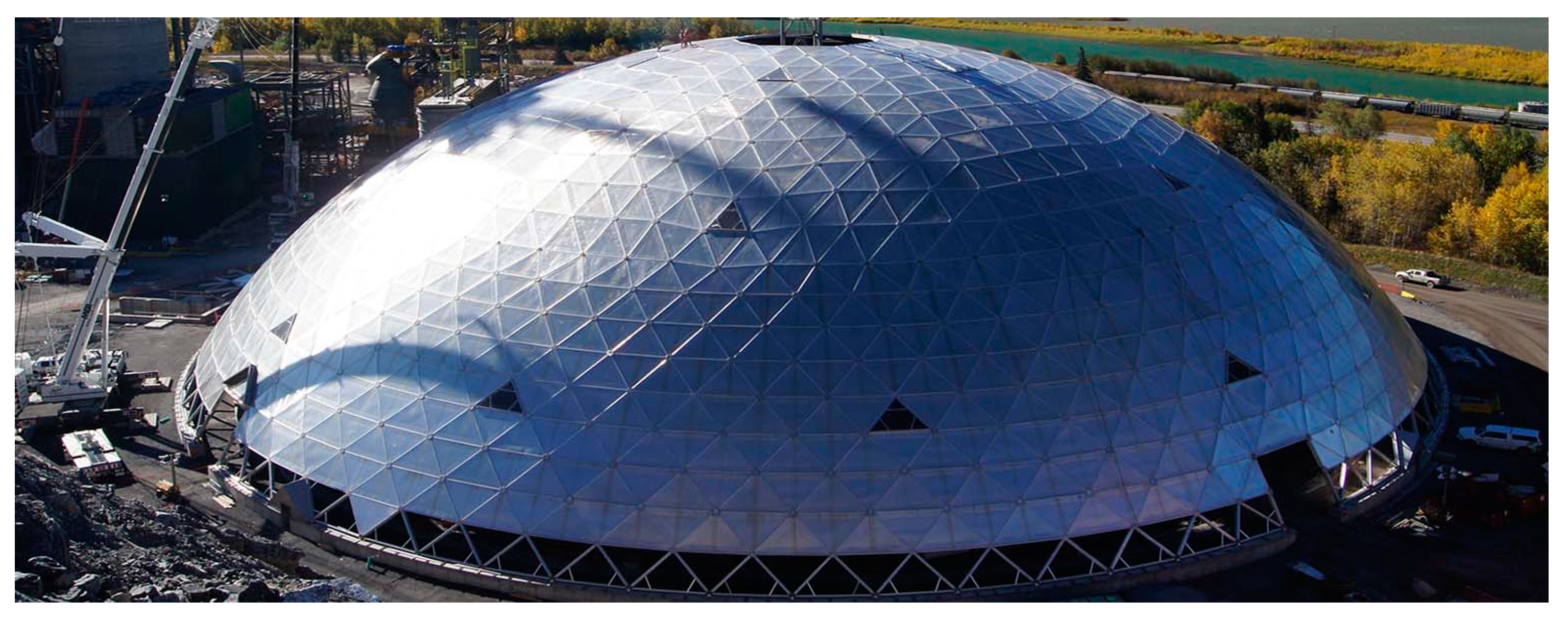
A hemispherical shell is widely used in large span structures, which have been constructed in large public buildings such as gymnasiums, exhibition centers, and opera houses [1,2]. Such curved shapes are often used for steel shells and rod structure as they are naturally strong structures, allowing wide areas to be spanned without the use of internal supports, giving an open, unobstructed interior. Figure 1 shows a geodesic dome for digital artwork that was established in 2014 [3]. The use of steel as a building material reduces both material costs and construction costs, as steel is relatively inexpensive and easily made into compound curves. The shell structure tends to be immensely strong and safe. For example, modern monolithic dome houses have resisted hurricanes and fires. In recent literature, there has been renewed interest in the problem of a hemispherical shell vibrating in contact with air or other fluids [4]. The vibrations of a structure induce local air movement, while the moving air and global atmospheric pressure affect the structure at the same time. Such phenomenon is called fluid–structure interaction (FSI) effect.

There are some publications in the literature devoted to the interaction of fluid and shell by theoretical approaches [5,6]. In the way of potential flow theory, Minami [7] derived the added mass ratio for a rectangular plate under the assumption that the vibration mode is simple harmonic. Actually, the researcher utilized the incompressible assumption so the obtained result was an added mass ratio. Wang [8] reanalyzed the same problem with the assumption that the structure vibrates as a quadratic function and raised another added mass formula. In both papers, the problem was actually treated as a one-dimensional model so that their method cannot be applied to two-dimensional (2D) and three-dimensional (3D) problems. Yadykin [9] studied the effect of the added mass of a thin shell vibrating in a stationary fluid through using the energy method, and the pressure of the shell was calculated by the thin-airfoil theory. Ping and Wei [10] studied the problem of a beam vibrating in the fluid based on the classical Fourier series, and reported the effects of the added mass ratio on the one-dimensional beam vibrating in non-viscous fluid.

Most of the research about the vibrations of shell in fluids commonly studied them by a numerical method, especially by the computation fluid dynamics (CFD) method [11,12]. Sorokin and Terentiev [13] studied the effect of the generation and transmission of the vibro-acoustic energy in an elastic cylindrical shell filled with water. They focused more on vibro-acoustic energy than the pressure. Chen et al. [14] studied the Guangzhou International Convention and Exhibition Center with dimensions that were 210 m wide and 457 m long. They studied the pressure distribution of the exhibition according to the wind tunnel test. Stolarski [15] conducted some research studies on the pressure of compressible squeeze film. In the study, the CFD method was used. Jeong and Kim [16,17] developed a Rayleigh–Ritz method to study a proportional hydroelastic vibration of two annular plates coupled with a bounded fluid. They considered the effects of the compressibility of the fluid and obtained a theoretical result that could predict the fluid-coupled frequencies well. Kubenko et al. [18] conducted a number of studies on a cylindrical shell submerged in an unbounded medium. They also assumed the fluid to be an incompressible fluid. Eftekhari [19] developed a differential quadrature method (DQM) to investigate the problem of the free vibration of circular plates in contact with fluid. Hu and Tang [20,21] investigated a simple-based monolithic implicit method for the strong-couple FSI problem. Their method may be used to analyze the vibration of the shell. These methods consist of several numerical approaches, but they offered little findings on a basis of theoretical analysis.

In spite of previous research on shells in contact with an incompressible fluid by experimental or numerical methods, very few studies on shells vibrating in compressible fluid have been performed. There have also been no attempts to tackle the problem of hemispherical shell vibration, which is highlighted in this paper. Moreover, up to now, very few studies have reported how many errors occurred owing to the incompressible fluid assumption. According to previous studies, our research is the first to consider the compressibility of fluid, which cannot be neglected. In the present paper, the pressure of a hemispherical surface vibrating under both compressible and incompressible fluid are analyzed using the Bessel function method. The principle of pressure on the shell surface is discussed, and some formulas about the velocity and pressure are highlighted. All of the results are verified using the calibrated numerical simulations. The outcome of this study will enable a novel analytical formulation that can be used to predict the vibration of a spherical shell structure interacting with fluids. This formulation can be used in the design and analysis of the structure in practice.

2. Control Equation and Solution

2.1. Formulation for Hemispherical Shell

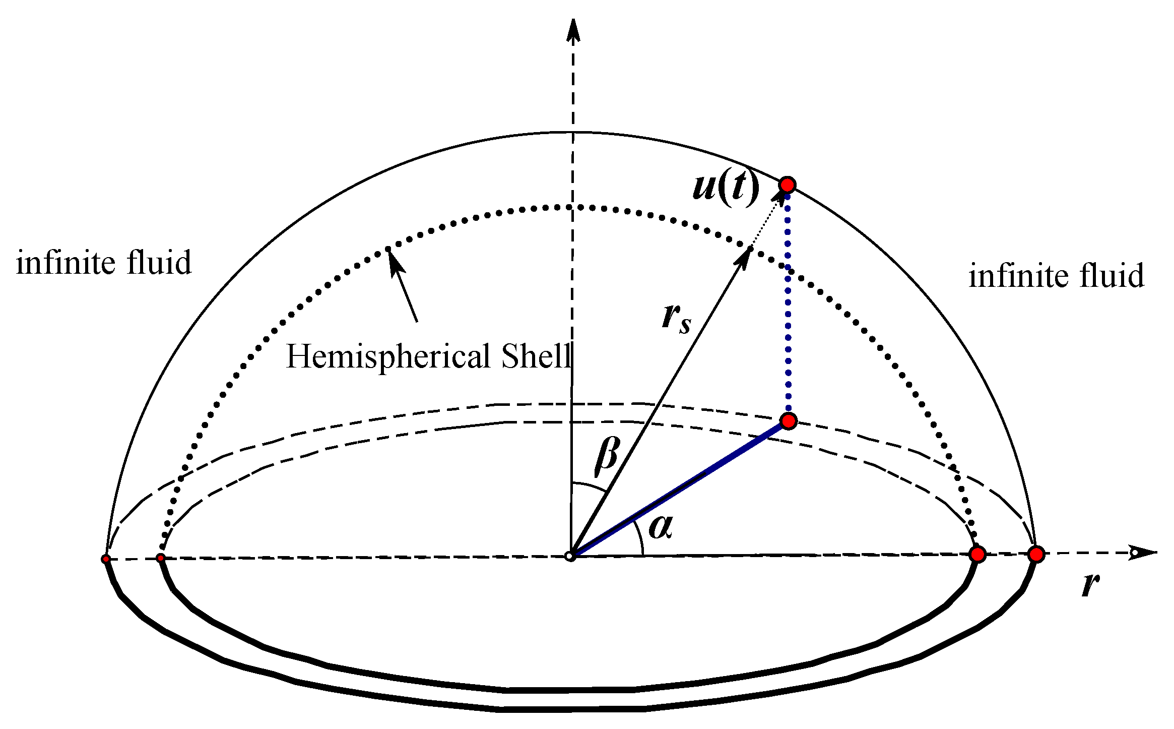
Figure 2 shows a mechanical model of a hemispherical shell vibrating in a radial direction in the unbounded fluid. Obviously, structure vibration affected the boundary of flow, while the pressure of flow affected the structure simultaneously. With an inviscid fluid hypothesis, the assumption of $p=c^2\rho$, and the character of axial symmetry, the FSI coupling equation can be simplified as follows [22], where $m$ represents the areal density of the shell, $U$ represents the displacement of vibration, $k$ represents the bending stiffness, $u$ represents the velocity of fluid in the radius direction, and $\Delta p$ represents the pressure differential between the upper surface and the bottom surface of the shell.

$$m\frac{{\partial }^{2}U}{{\partial }^{2}t}+k\cdot {\nabla }^{4}U+\Delta p=0$$

(1)

$$\frac{\partial \rho }{\partial t}+\frac{\partial \rho \cdot u}{\partial r}+\frac{2\rho \cdot u}{r}=0$$

(2)

$$\frac{\partial u}{\partial t}+u\frac{\partial u}{\partial r}+\frac{1}{\rho }\frac{\partial p}{\partial r}=0$$

(3)

Equation (1) is the structural control equation of vibration. The first term of Equation (1) presents the inertial force (pressure) derived from the acceleration of motion, and the second term of Equation (1) shows the elastic force contributed from the deformation of the shell. According to Newton’s second law, the combination of inertial force, elastic force, and pressure without damping force are in the condition of balance. The boundary conditions can be written as Equation (4), where the first term condition means the displacement is zero at the initial time, and the second term shows that the initial velocity of the shell is in compliance to the $u_s(0)$ at the initial time.

$${U|}_{t=0}=0,{\frac{\partial U}{\partial t}|}_{t=0}=u_s(0).$$

(4)

Equations (2) and (3) are fluid control equations, which are well known as Naiver–Stokes equations (3D axial symmetry), where the density, static pressure, sound speed, and velocity of the fluid is denoted by $\rho$, $p$, $c$, and $u$, respectively. Equation (2) was derived from the conservation of mass, and Equation (3) was deduced from the conservation of momentum. Let:

$$\frac{\partial U}{\partial t}=u_s(t),$$

(5)

The velocity of fluid boundary vibration is, u = u_s(t). Here, it assumes that |u_s| = c. Therefore, the boundary conditions can be rewritten as Equation (6), where, the first term shows that the boundary of fluid is just the position of the shell, and both the second and third terms present that on the boundary of the far field, the velocity and pressure are approximate to the initial condition 0, $p_0$, respectively.

$${u|}_{r=r_s}=u_s(t),{u|}_{r=R->\infty }=0,{p|}_{r=R->\infty }=p_0$$

(6)

According to the physical conditions, the boundary of the fluid is the structural shell itself actually; thus, the initial value of the radius is the radius of the hemispherical shell, $r_s$, therefore:

$$r_s(t)=r_s+U(t),$$

(7)

where $r_s(t)$ is the radius of the fluid boundary, which varies with time. Since $U$ is taken into account in a small value, $r_s(t)$ can be denoted as $r_s$. The initial condition can be expressed by:

$${\rho |}_{t=0}={\rho }_0,{p|}_{t=0}=p_0$$

(8)

2.2. Solution on the Compressible Fluid Case

Using the Fourier series method, the velocity can be written in a harmonic function with a frequency of $\omega$. This implies that:

$$\frac{{\partial }^{2}u}{\partial t^2}=-{\omega }^{2}u$$

(9)

For the physical property of the fluid, the density changes slightly, but the change of density over time and space cannot be neglected. Thus, in this paper, the density is assumed to be a constant as ${\rho }_o$, but the changes of density over time and space have to be considered in the solution. From Equation (2), pressure can be obtained by the integration between limits from $r$ to the unbounded position:

$$\Delta p=p-p_0=-{\rho }_o{\displaystyle {\int }_r^{\infty }\frac{\partial u}{\partial t}}dr+\frac{{\rho }_o}{2}{u}^2,$$

(10)

From Equation (10), it is found that the pressure comes from two parts: the local acceleration, which is the velocity changes with respect to time, and the convective acceleration, which is the change in velocity with respect to space. It should be noted that there is only one boundary condition with respect to the pressure as prescribed in Equation (6). Therefore, the pressure at the position of $r$ is an unknown value. This implies that there is an arbitrary constant that needs to be determined in Equation (10). For the assumption of $u_s\ll c$, the second term of Equation (10) is very small. After neglecting the convective acceleration (the second term) and substituting the local acceleration (the first term) to the continuous equation of Equation (2), it can be obtained as follows:

$$-\frac{{\omega }^2}{c^2}{\displaystyle {\int }_r^{\infty }u}dr+\frac{\partial u}{\partial r}+\frac{2u}{r}=0.$$

(11)

Equation (11) can be simplified as Equation (12) below after a derivative by $r$. Having an arbitrary constant in pressure discussed above, two boundary conditions are necessary to solve Equation (11), although it is a first order differential equation. The two boundary conditions are the same as Equation (12):

$$\frac{{\partial }^{2}u}{\partial r^2}+\frac{2}{r}\frac{\partial u}{\partial r}+(\frac{{\omega }^2}{c^2}-\frac{2}{r^2})u=0,$$

(12)

Let $s=\frac{\omega }{c}r$, and the above equation can be expressed in terms of the classical Bessel equation as follows:

$$s^2\frac{{\partial }^{2}u}{\partial s^2}+2s\frac{\partial u}{\partial s}+(s^2-1\times 2)u=0.$$

(13)

Equation (13) is a classical Bessel equation, so the solution can be derived as:

$$u=A\cdot j_1(s)+B\cdot y_1(s),$$

(14)

where $A$ and $B$ are the arbitrary functions of the time, and $j_1(s)$, $y_1(s)$ are the first and the second-order Bessel function, respectively. Applying the boundary conditions into Equation (14), it can be rewritten as Equation (15) shows:

$$\{\begin{array}{l}{A\cdot j_1(s)+B\cdot y_1(s)|}_{r=r_s}=u_s(t)\\ {A\cdot j_1(s)+B\cdot y_1(s)|}_{r=R->\infty }=0\end{array}$$

(15)

Thus, to get the exact solution, there are only $A$ and $B$ left to be confirmed. It should be noted that when $r=R\to \infty$, both $j_1(s_R)$ and $y_1(s_R)$ converge to zero. Therefore, the second term of the boundary condition is satisfied naturally. In such cases, taking into account that $u$ is a harmonic function, it can be assumed that:

$$A=C\cdot \cos (\omega t+\phi ),B=C\cdot \sin (\omega t+\phi ).$$

(16)

According to the first term of the boundary conditions, the amplitude and phase angle will be equal to that of initial vibration, so that $A$ and $B$ can be confirmed. In addition, it is found that the solution can be determined totally by the boundary condition $u_s(t)$.

2.3. The Analysis of the Velocity

Due to the physical boundary conditions, the vibration at the boundary can be expressed as:

$$u_s(t)=D\cdot \sin (\omega t),$$

(17)

where $D$ represents the amplitude of vibration. So, the first term of the boundary condition can be expressed as Equation (18):

$$C\cdot [\cos (\omega t+\phi )\cdot j_1(s_r)+\sin (\omega t+\phi )\cdot y_1(s_r)]=u_s(t),$$

(18)

Afterward, it may be simplified as follows:

$$C\sqrt{j_1^2(s_r)+y_1^2(s_r)}\sin (\omega t+\phi +\varphi )=D\cdot \sin (\omega t),$$

(19)

where, $s_r=\frac{\omega }{c}{r}_r$, and $\tan (\varphi )=\frac{j_1(s_r)}{y_1(s_r)}$. Furthermore, it may be obtained that:

$$C=\frac{D}{\sqrt{j_1^2(s_r)+y_1^2(s_r)}},\phi =-\varphi =-\arctan [\frac{j_1(s_r)}{y_1(s_r)}].$$

(20)

By the nature of the Bessel function [23,24], if $s$ is very large, then there are:

$$\{\begin{array}{l}{j}_1(s)=\frac{\cos (s-\pi )}{s}\\ y_1(s)=\frac{\sin (s-\pi )}{s}\end{array},$$

(21)

Finally, the solution can be derived as Equation (22):

$$u=\frac{c}{\omega }\frac{D}{\sqrt{j_1^2(s_r)+y_1^2(s_r)}}\frac{\cos (\omega t-\frac{\omega }{c}r+\pi -\phi )}{r}.$$

(22)

Accordingly, it can be concluded that the characteristic of vibration at time $t_0$ will transfer to the position $r=ct$ with the same frequency between time $t$, and the amplitude will be decreased with the rate of $\raisebox{1ex}{$1$}\!\left/ \!\raisebox{-1ex}{$r$}\right.$.

2.4. The Analysis of the Pressure

By the characters of the Bessel function, it also can be written that:

$$\{\begin{array}{l}{\displaystyle \int j_1(r)}dr=-j_0(r)\\ {\displaystyle \int y_1(r)}dr=-y_0(r)\end{array},\{\begin{array}{l}\underset{r\to \infty }{\lim }{j}_1(r)=0\\ \underset{r\to \infty }{\lim }{y}_1(r)=0\end{array},$$

(23)

Thus, the formula about pressure can be obtained:

$$\Delta p={\rho }_{o}c\cdot D\frac{\cos (\omega t+\phi +\frac{\pi }{2})j_0(s)+\sin (\omega t+\phi +\frac{\pi }{2})y_0(s)}{\sqrt{j_1^2(s_r)+y_1^2(s_r)}},$$

(24)

where $s$, $\phi$, $D$ are the same as the Section 2.3. if $s$ is large, there are:

$$j_0(s)=\cos (s-\frac{\pi }{2})/s, y_0(s)=\sin (s-\frac{\pi }{2})/s$$

(25)

Finally, the solution of the pressure can be induced:

$$\Delta p=\frac{{\rho }_o{c}^2}{\omega }\frac{\left|u_s\right|}{\sqrt{j_1^2(s_r)+y_1^2(s_r)}}\frac{\cos [\omega (t-\frac{r}{c})+\phi -\pi ]}{r}={\rho }_{o}c\cdot u.$$

(26)

It can be seen from Equation (26) that the pressure is proportional to the velocity of vibration and the ratio is the product of the density and the sound speed. Furthermore, according to Equation (22), the convective acceleration is $\raisebox{1ex}{$1$}\!\left/ \!\raisebox{-1ex}{$2$}\right.{\rho }_o{u}^2$, which is the commonly used pressure formula derived by Bernoulli law [25]. Besides, compared to Equation (26), the value of the convective acceleration is very small. This means that neglecting the value of convective acceleration cannot cause a large error.

2.5. Incompressible Fluid Solution

As for a comparison, it is necessary to consider the model of a shell vibrating in the incompressible fluid. The control equation can be expressed as follows:

$$m\frac{{\partial }^{2}U}{{\partial }^{2}t}+k\cdot {\nabla }^{4}U+\Delta p=0,$$

(27)

$$\frac{\partial u}{\partial r}+\frac{2u}{r}=0,$$

(28)

$$\frac{\partial u}{\partial t}+u\frac{\partial u}{\partial r}+\frac{1}{{\rho }_o}\frac{\partial p}{\partial r}=0,$$

(29)

Equation (27) is the structural control equation, which is the same as Equation (1). Equation (28) is the continuity equation with the constant density. Equation (29) is the equation for the conservation of momentum. The symbols and the boundary conditions of structure are the same as Equation (4), whilst the boundary of the fluid domain is as follows:

$${u|}_{r=r_s}=u_s(t),{u|}_{r=R->\infty }=0, {p|}_{r=R->\infty }=p_0$$

(30)

According to the continuity equation, it may be concluded as Equation (31):

$$u(r,t)=\frac{r_s^2}{r^2}{u}_s(t),$$

(31)

While according to the momentum equation, it can be written as:

$$p(r)=-{\rho }_0\frac{\partial u_s}{\partial t}\frac{r_s^2}{r}-\frac{1}{2}\frac{r_s^4}{r^4}{u}_s^2+C.$$

(32)

Substituting the boundary condition of the far field to Equation (32), it can be found that:

$$\Delta p=p-p_0={\rho }_0\frac{r_s^2}{r}\frac{\partial u_s}{\partial t}+\frac{1}{2}{\rho }_0{u}_s^2\frac{r_s^4}{r^4}.$$

(33)

From the solution of Equation (31), in the condition of incompressible fluid, it is found that the motion of boundary will transfer to the far field simultaneously, and the amplitude decreases with the rate of $\raisebox{1ex}{$1$}\!\left/ \!\raisebox{-1ex}{$r^2$}\right.$. According to Equation (33), it can be observed that the pressure is contributed from two parts [26]. The first term of pressure can be seen as added mass, and the second term is also convective acceleration, which is the same as Equation (5). The pressure under the shell is $\Delta p={\rho }_0{r}_s\frac{\partial u_s}{\partial t}+\frac{1}{2}{\rho }_0{u}_s^2$, which is very different to the solution of compressible fluid condition.

2.6. Discussion

For the incompressible fluid condition, Equation (33) shows that it has an important influence, as the incompressible assumption was adopted, and the pressure is contributed from two parts. The first part is the local acceleration, which is proportional to both the boundary acceleration and the reciprocal of the radius of the fluid domain. Another part is proportional to the square of the fluid velocity. As for compressible fluid, according to the solution, $\Delta p={\rho }_{o}c\cdot u$, it can be concluded that the pressure is proportional to the velocity of fluid. The ratio is the product of the sound speed and the density. In such case, it can be obtained from Equation (1) that the pressure effect of fluid on the structure is equivalent to the viscous damping whose value is ${\rho }_{o}c$, exactly.

In the physical sense, it can be seen that between times $\Delta t$, the amount of fluid that can be squeezed by the structure is $\raisebox{1ex}{$4$}\!\left/ \!\raisebox{-1ex}{$3$}\right.\pi [{(r_s+u_s\Delta t)}^3-r_s^3)]$, and can be spread to the range of $\raisebox{1ex}{$4$}\!\left/ \!\raisebox{-1ex}{$3$}\right.\pi [{(r_s+c\Delta t)}^3-r_s^3]$. When $\Delta t\to 0$, the fluid compression ratio is:

$$\underset{\Delta t\to 0}{\lim }\frac{\raisebox{1ex}{$4$}\!\left/ \!\raisebox{-1ex}{$3$}\right.\pi [{(r_s+u_s\Delta t)}^3-r_s^3)]}{\raisebox{1ex}{$4$}\!\left/ \!\raisebox{-1ex}{$3$}\right.\pi [{(r_s+c\Delta t)}^3-r_s^3]}=\frac{u_s}{c}$$

(34)

Moreover, the fluid compression modulus is ${\rho }_o{c}^2$, Therefore, according to Hooke’s law, the pressure of compressible fluid is:

$$p=c^2\cdot \frac{u_s}{c}={\rho }_{o}c\cdot u_s,$$

(35)

The pressure of compressible fluid is identical to Equation (26) exactly. The discussion above shows that in the condition of compressible fluid, the motion of boundary propagates to the far field at the speed of sound. At the beginning, the motion of the shell compresses the air (fluid), which will be transferred to the far field afterward. The compression of air produces the local acceleration pressure, which is proportional to the fluid velocity.

3. Numerical Validation

3.1. CFD Method

It is well-known that the second-order method is the most stable discretization scheme, which is derived by Taylor’s series:

$$\frac{{\partial }^{2}u}{\partial x^2}=\frac{\partial }{\partial }[\frac{\partial u}{\partial x}]=\underset{\Delta x->0}{lim}\frac{{(\partial u/\partial x)}_{i+1/2}-{(\partial u/\partial x)}_{i-1/2}}{\Delta x}\approx \frac{u_{i+1}-2u_i+u_{i-1}}{{(\Delta x)}^2}+O(\Delta x^2)$$

(36)

$$\frac{{\partial }^{2}u}{\partial x\partial y}\approx \frac{u_{i+1,j+1}-u_{i+1,j-1}-u_{i-1,j+1}+u_{i-1,j-1}}{4\Delta x\Delta y}+O(\Delta x^2,\Delta y^2)$$

(37)

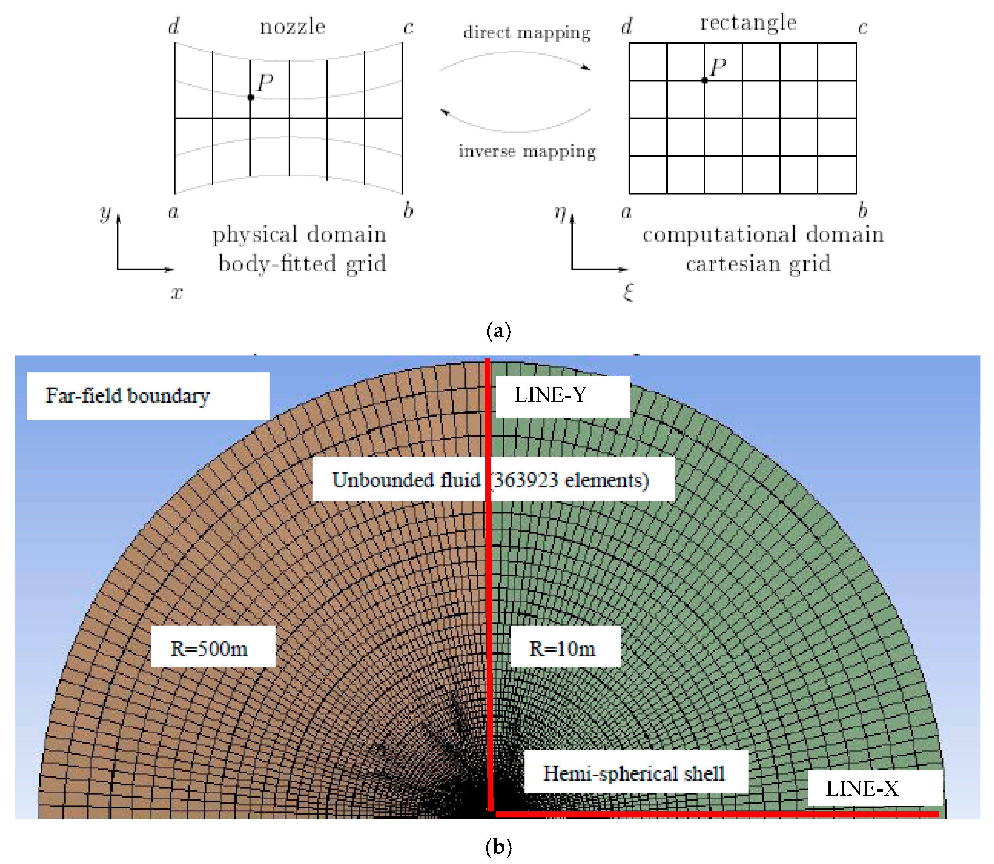
Equations (36) and (37) are one and two-dimensional schemes, respectively, in which $u$ is the value of physical quantities such as velocity and pressure, and $x,y$ are the coordinates. Usually, the grid will not be the rectangular shape. Let the transformation of domain be as Equation (36), shown in Figure 3a.

$$\xi =\xi (x,y),\eta =\eta (x,y)$$

(38)

In that case, the differential can be obtained by the chain rule, and the second-order differential cab be rewritten as Equations (39) and (40):

$$\frac{{\partial }^{2}u}{\partial x^2}=\frac{\partial u}{\partial \xi }\frac{{\partial }^2\xi }{\partial x^2}+\frac{\partial u}{\partial \eta }\frac{{\partial }^2\eta }{\partial x^2}+2\frac{{\partial }^{2}u}{\partial \xi \partial \eta }\frac{\partial \xi }{\partial x}\frac{\partial \eta }{\partial x}+\frac{{\partial }^{2}u}{\partial {\xi }^2}{(\frac{\partial \xi }{\partial x})}^2+\frac{{\partial }^{2}u}{\partial {\eta }^2}{(\frac{\partial \eta }{\partial x})}^2$$

(39)

$$\frac{{\partial }^{2}u}{\partial y^2}=\frac{\partial u}{\partial \xi }\frac{{\partial }^2\xi }{\partial y^2}+\frac{\partial u}{\partial \eta }\frac{{\partial }^2\eta }{\partial y^2}+2\frac{{\partial }^{2}u}{\partial \xi \partial \eta }\frac{\partial \xi }{\partial y}\frac{\partial \eta }{\partial y}+\frac{{\partial }^{2}u}{\partial {\xi }^2}{(\frac{\partial \xi }{\partial y})}^2+\frac{{\partial }^{2}u}{\partial {\eta }^2}{(\frac{\partial \eta }{\partial y})}^2$$

(40)

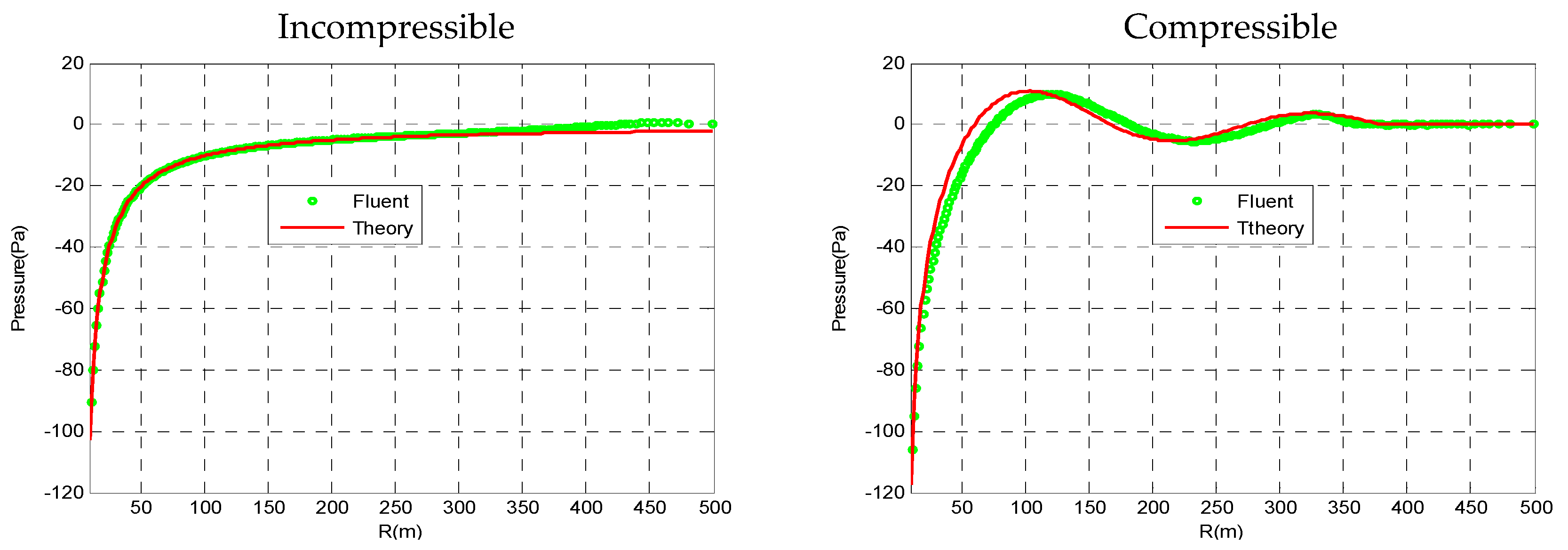
On the basis of the preceding analysis, in order to find and check the validity of the theory, a hemispherical shell submerged in unbounded fluid was examined using a CFD analysis using a commercial computer code, ANSYS (release 17.0, Ansys Company, Canonsburg, PA, USA) [27]. The CFD model has the identical shell geometry, boundary conditions, and material properties that will be used in the theoretical calculation. Similar applications can be found in some papers [28,29]. The radius of the hemispherical shell is set to 10 m, and the unbounded fluid is simulated as a far field boundary whose radius is 500 m (see Figure 3b). The physical properties of the fluid are as follows: density = 1.225 kg/m³, sound velocity c = 340 m/s. The viscosity of the fluid is neglected in both the theoretical analysis and the CFD calculation. The purpose of the present paper is to verify the principle of pressure under the vibration of the shell. The movement of the hemispherical shell was set as uniform vibration in the radial direction, which was also the boundary of the fluid. As for the numerical simulation parameters, the far field boundary is set to be the pressure far field, reference pressure to zero, movement boundary to U(t) = sin(10t), calculating time to 1.0 s, and the delta-time to 0.001 s. A simple scheme second-order method was accepted for the CFD simulation, and the initial condition of fluid was set to be stationary. For comparison, both the compressible fluid case and the incompressible fluid case were carried out. To verify the solution, the line from $r_s$ to $R$, which data was obtained from, is shown as LINE-X in Figure 3b.

In order to demonstrate the influence of the discretization, the numerical result with different meshing sizes is displayed.

Table 1. The total energy with different densities of mesh.

Density of Shell Mesh (cm)	2.0	1.0	0.8	0.5	0.3	0.2	0.1
Total Energy (104 J)	4.52	4.21	3.93	3.90	3.89	3.88	3.88

shows the comparison of the total energy of all over the fluid at time = 0.2 s with different density of shell mesh. Since the results of size = 0.2 m and size = 0.1 m are the same, the size of 0.2 m has been adopted in this paper. After meshing, there are 363,923 structural hexahedron elements.

3.2. Velocity Results

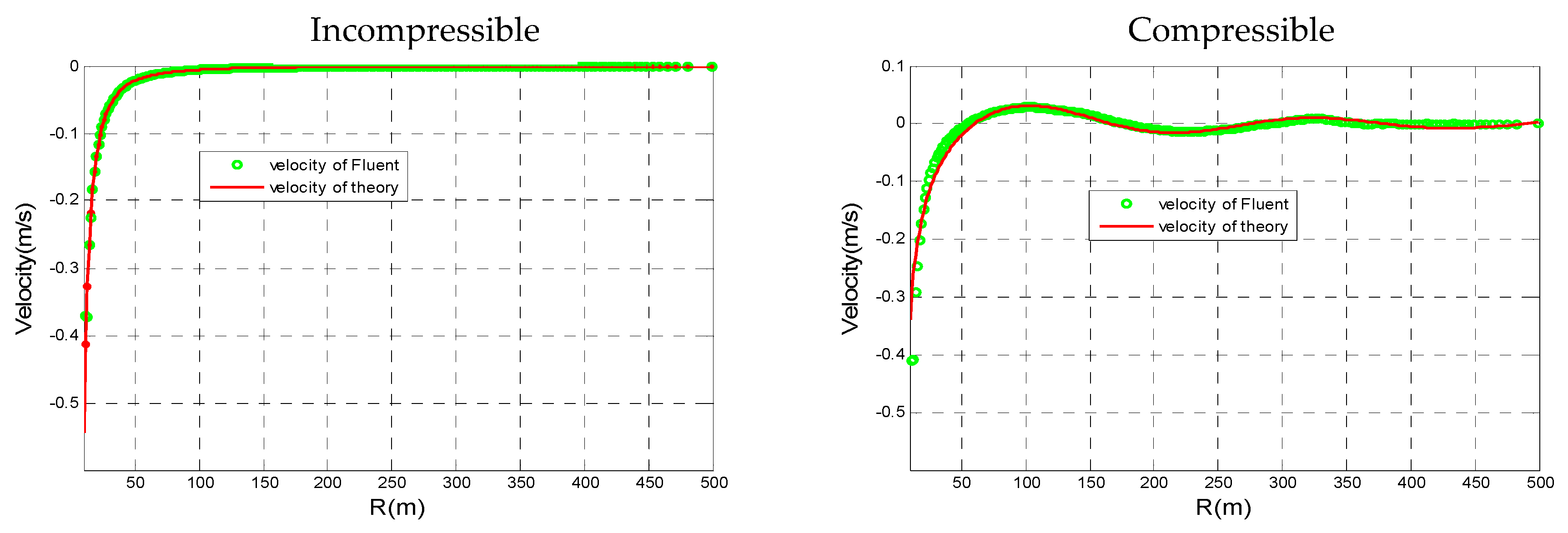
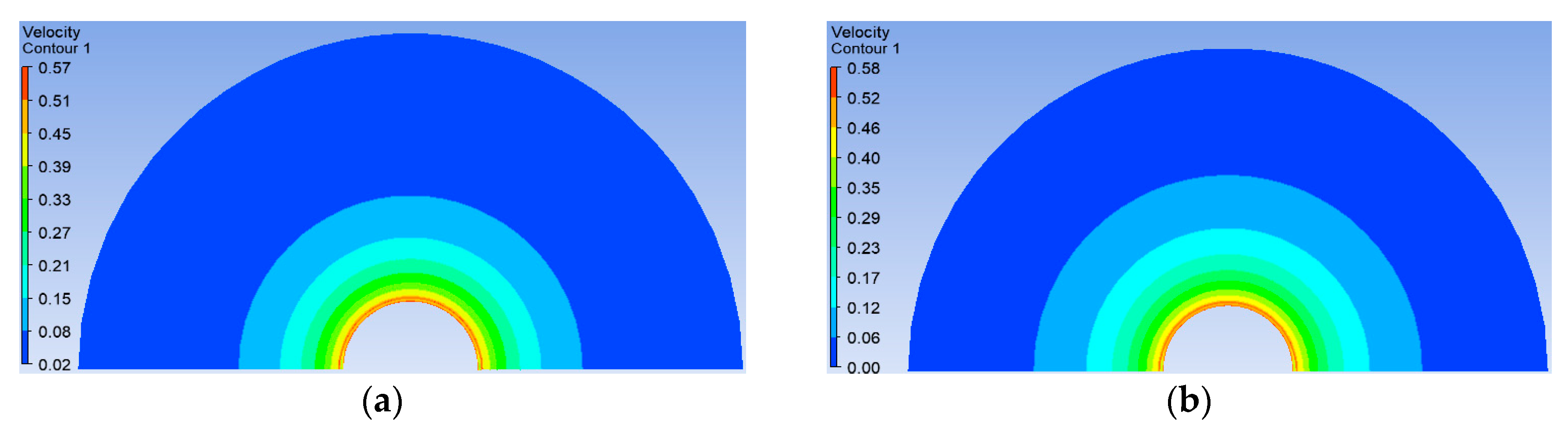
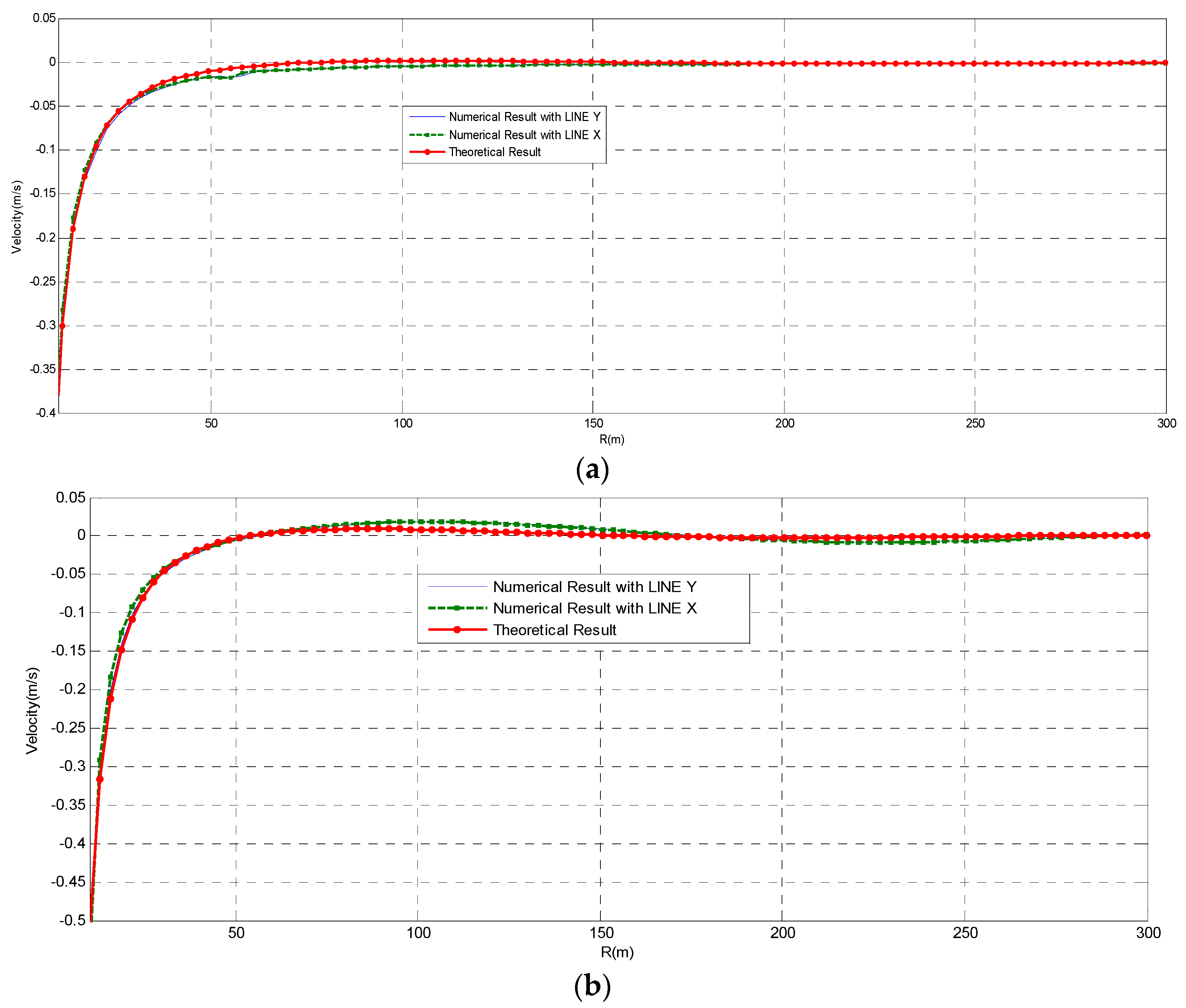
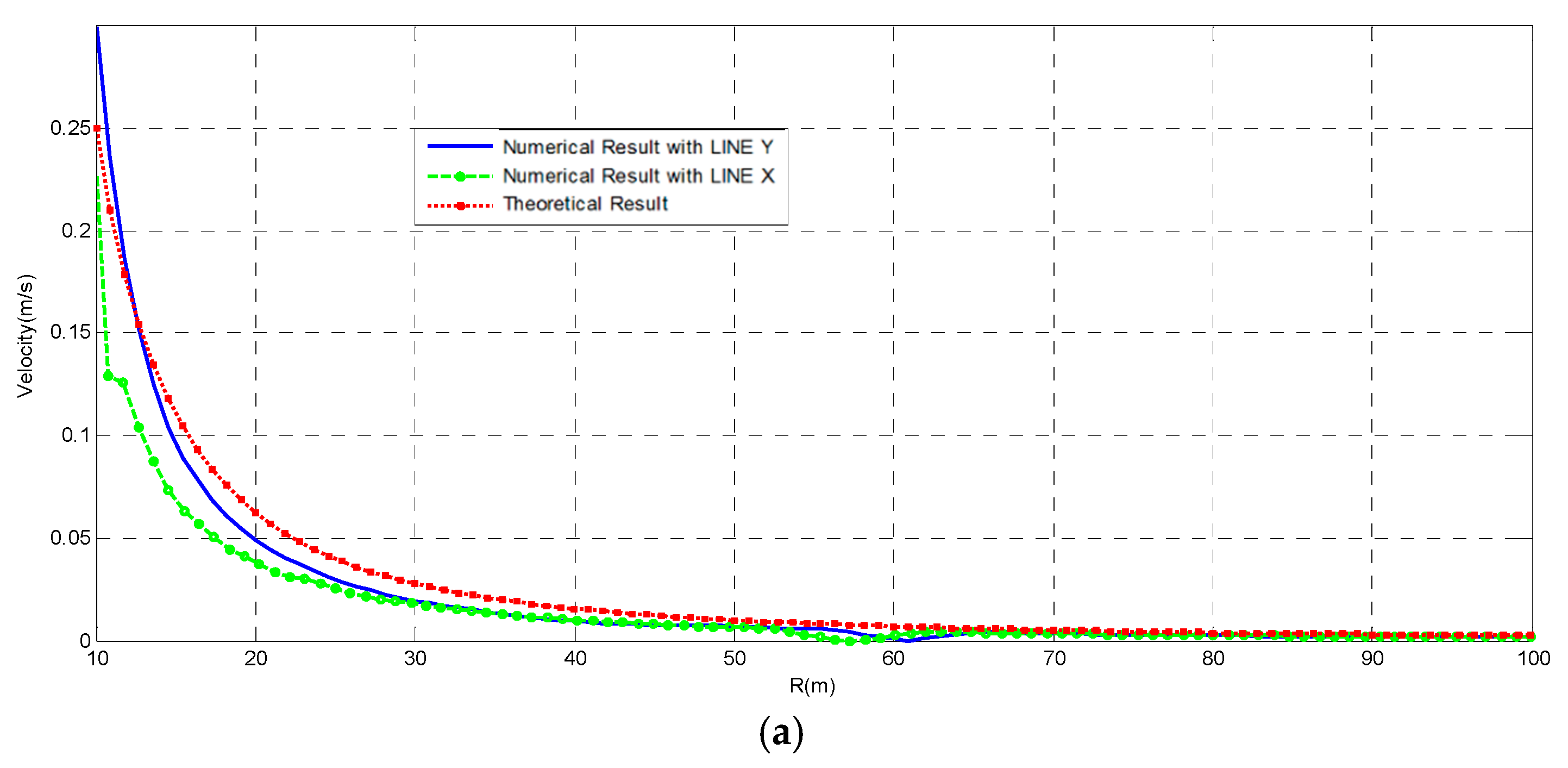
Figure 4 shows the relationship of the velocity versus radii, which are the results under the incompressible/compressible assumption at $t=$ 1.0 s. From both the left graph and the right graph, it can be seen that the analytical solution is in very good agreement with the numerical solution. The correlation coefficient in the left and right plot is 0.987 and 0.973, respectively. From the theoretical solution, boundary vibration is transmitted to the whole flow field in an instant under the incompressible assumption. Meanwhile, in the compressible condition, the transmission of the boundary motion to a far field needs a period of time.

Compared with both left and right plot in Figure 5, it can be found that the velocity of fluid in the incompressible fluid is a function of radii, which decreases with the function of $\raisebox{1ex}{$1$}\!\left/ \!\raisebox{-1ex}{$r^2$}\right.$. Therefore, it is found that the velocity far away from boundary shell trends to converge to zero quickly. On the other hand, the velocity in the compressible fluid is a function of both radii and time and the periodicity of radius from formula is $\raisebox{1ex}{$2\pi c$}\!\left/ \!\raisebox{-1ex}{$\omega $}\right.$ = 213, which is verified by the result in Figure 4 (left). Besides, the velocity amplitude decreases with the function of $\raisebox{1ex}{$1$}\!\left/ \!\raisebox{-1ex}{$r$}\right.$c, which is slower than that in the incompressible fluid condition.

3.3. Pressure Results

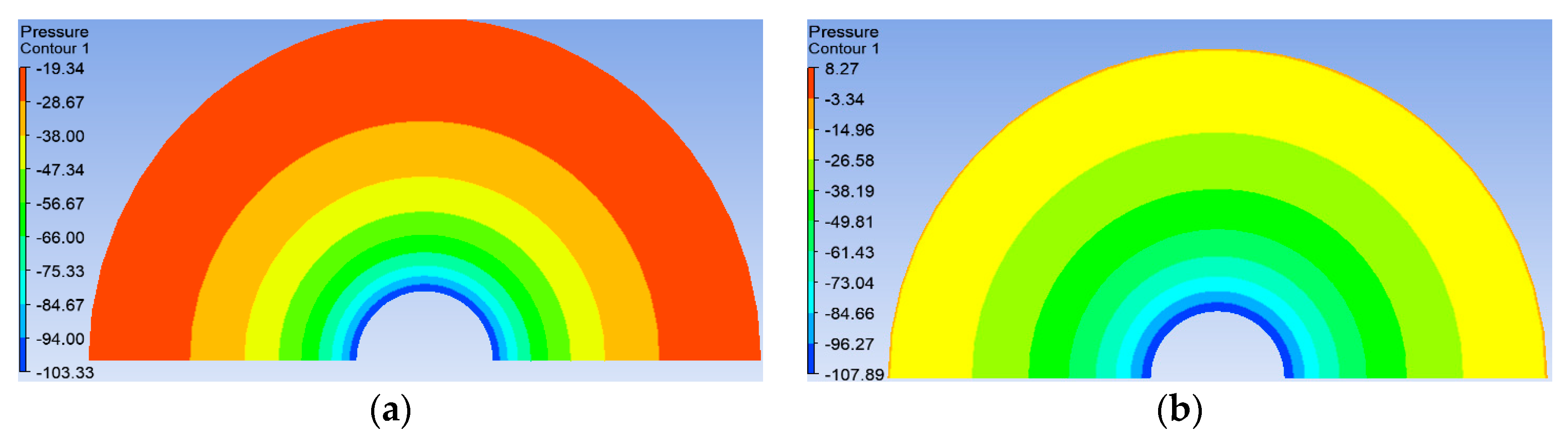
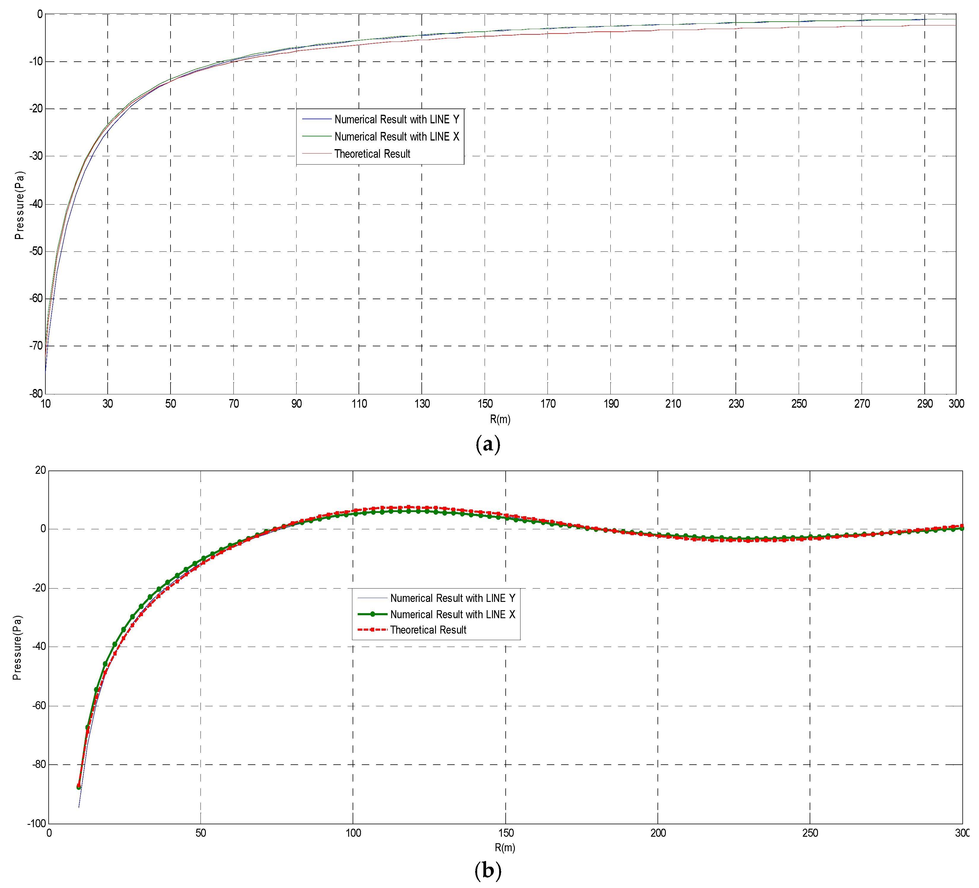
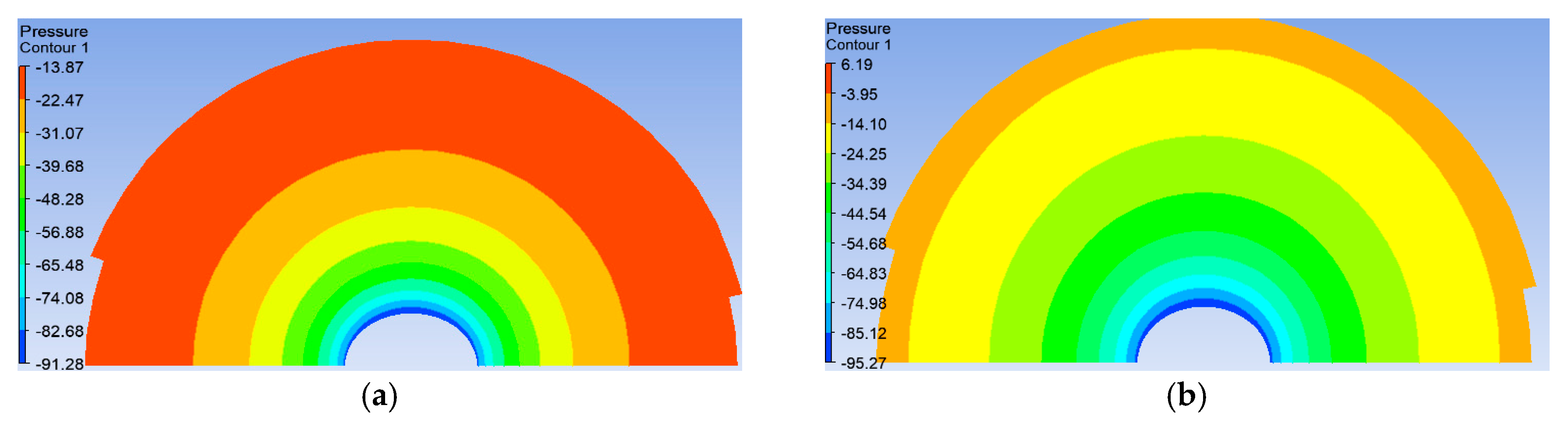
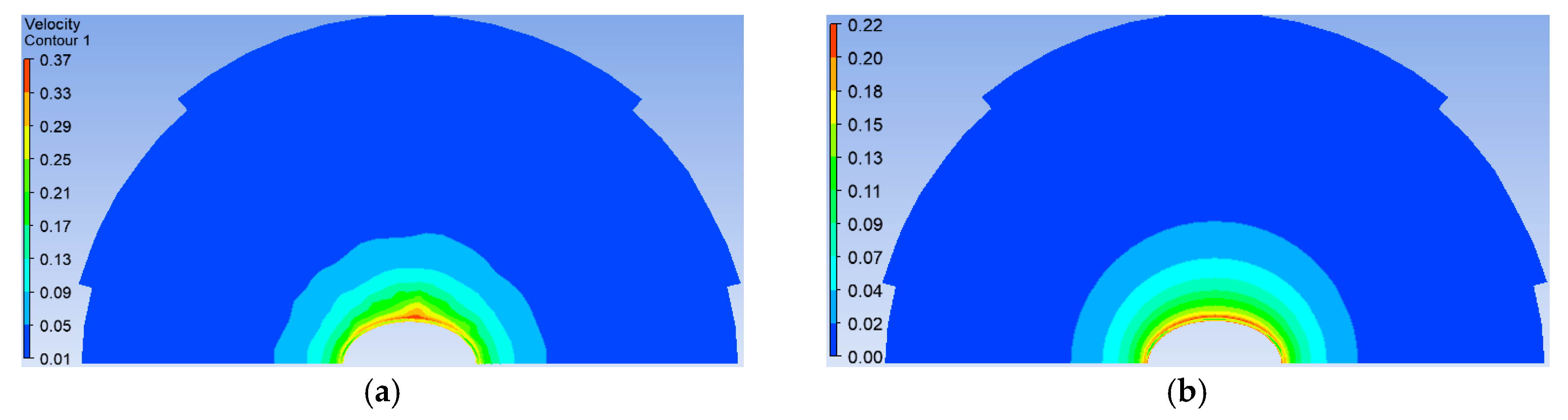
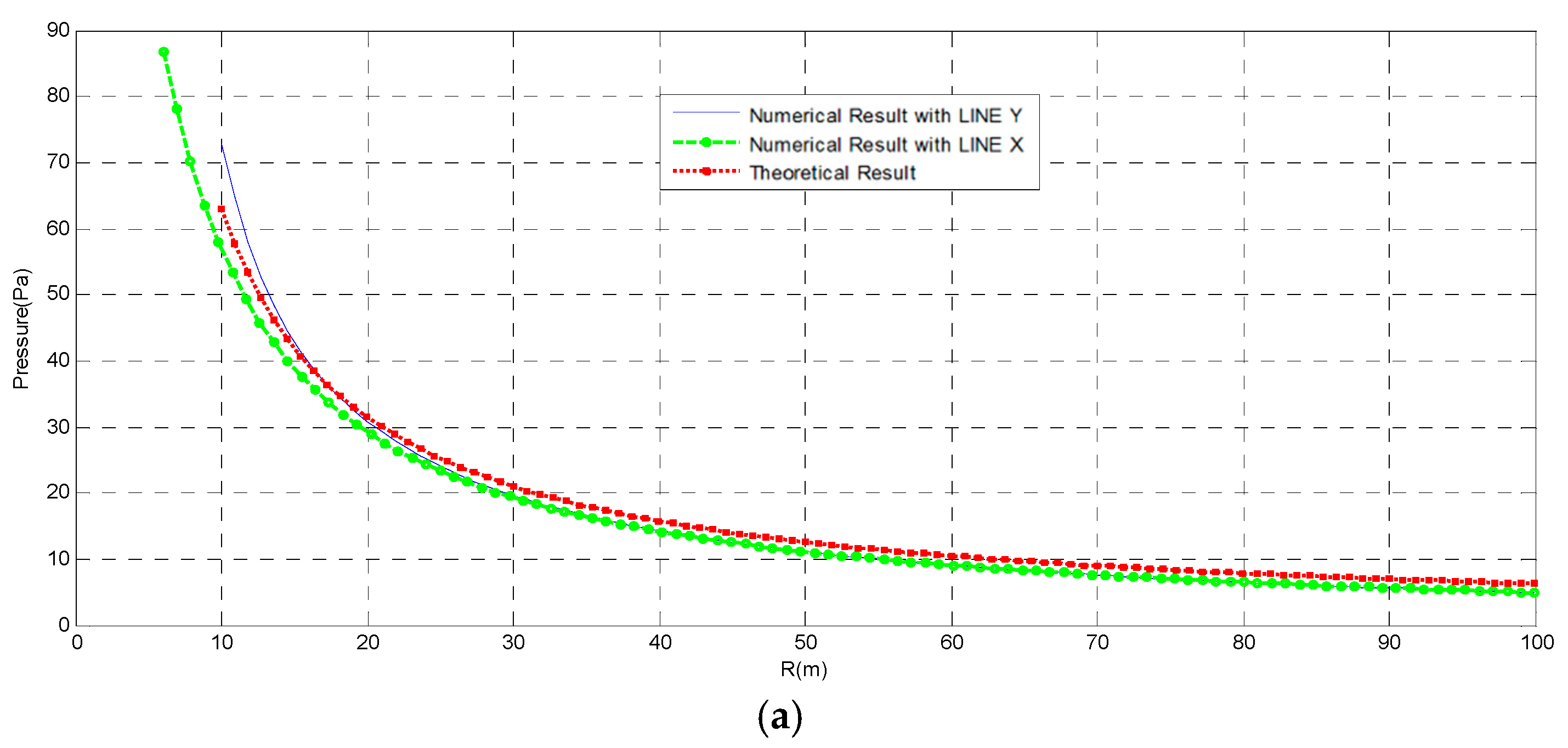
Figure 6 illustrates the comparison of theoretical and numerical solutions of the pressure under the incompressible and compressible flow. The analytical solution and numerical solution are in a very good agreement. The correlation coefficient in the left and right plot is 0.978 and 0.966, respectively. Particularly, for incompressible fluid, the numerical solution is almost identical to the analytical result. On the condition of compressible fluid, the numerical solution is almost consistent with the theoretical solution at the boundary zone.

Compared with both the left and right plots, it can be found that the pressure of fluid in the incompressible fluid is a function of radii, which decreases with the function of $\raisebox{1ex}{$1$}\!\left/ \!\raisebox{-1ex}{$r$}\right.$. Conversely, the pressure of fluid in the compressible fluid is a function of velocity, which can be rationalized by both of the right plots in Figure 6 and Figure 7.

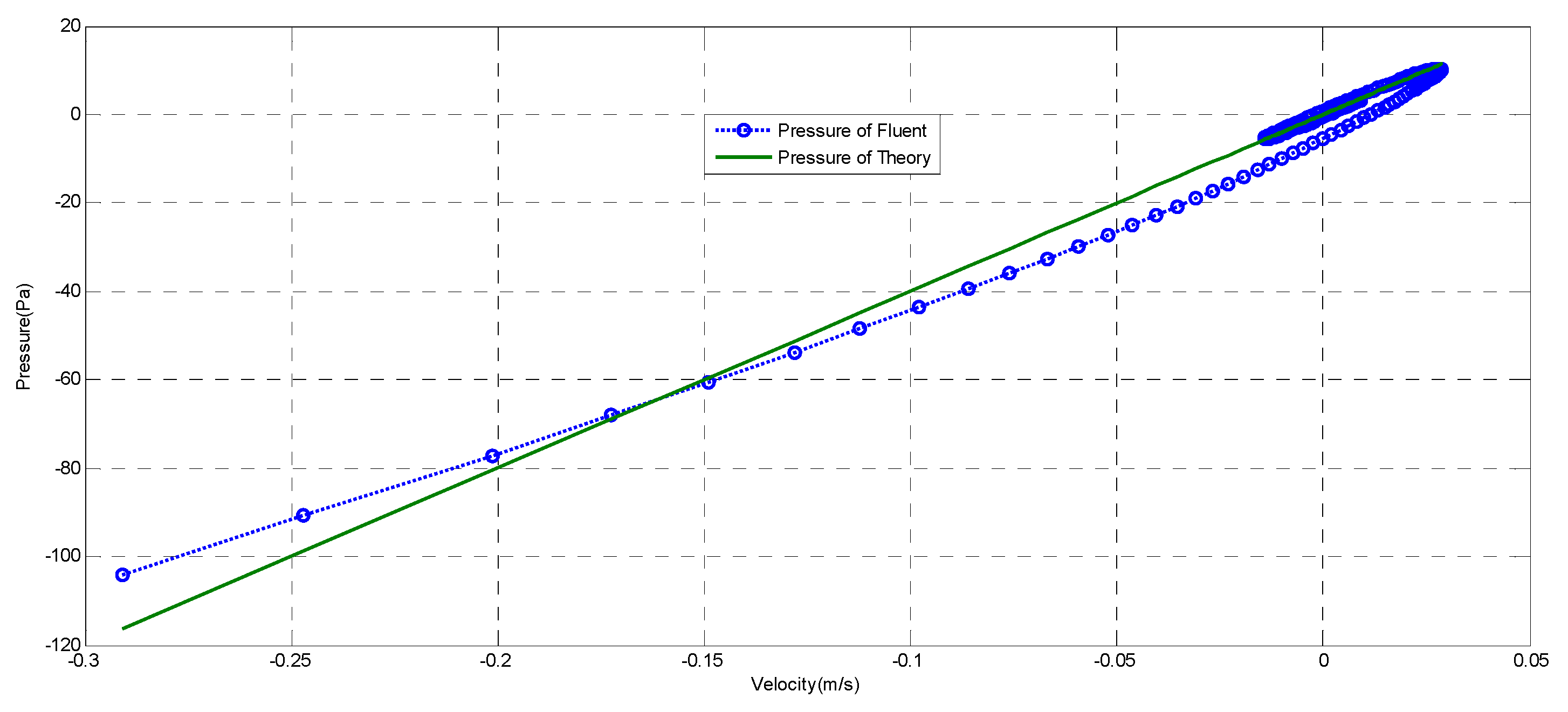
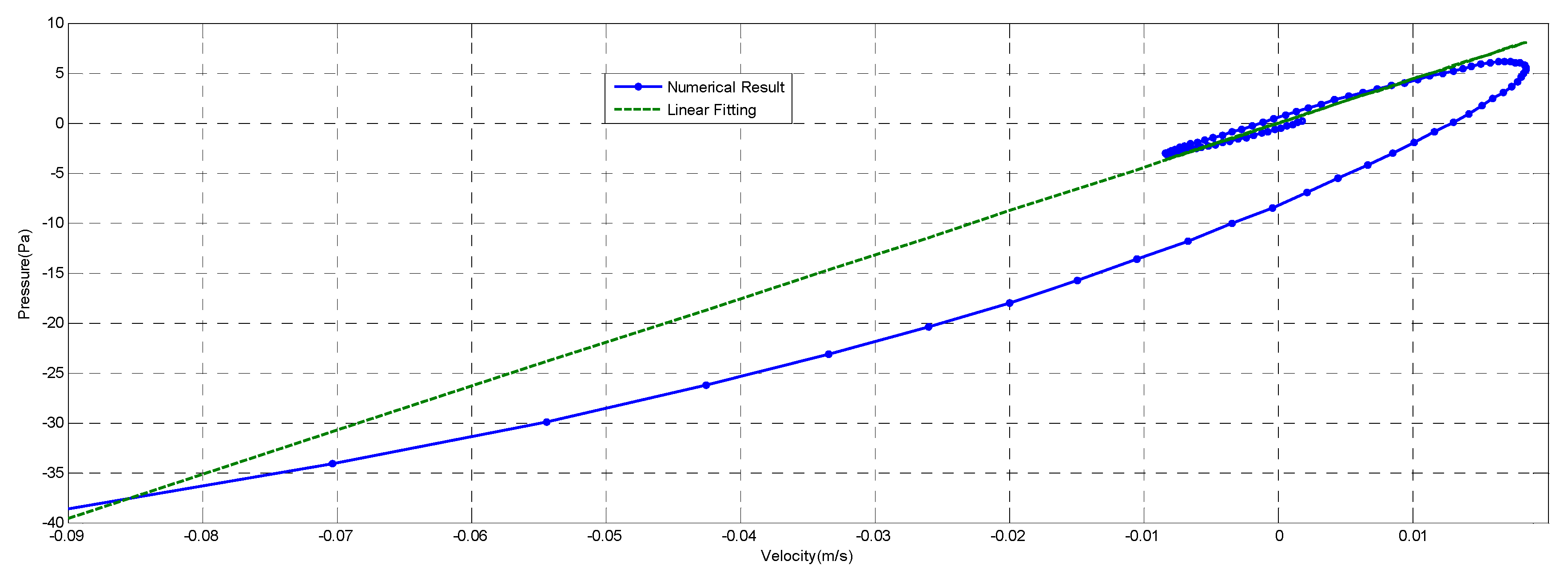
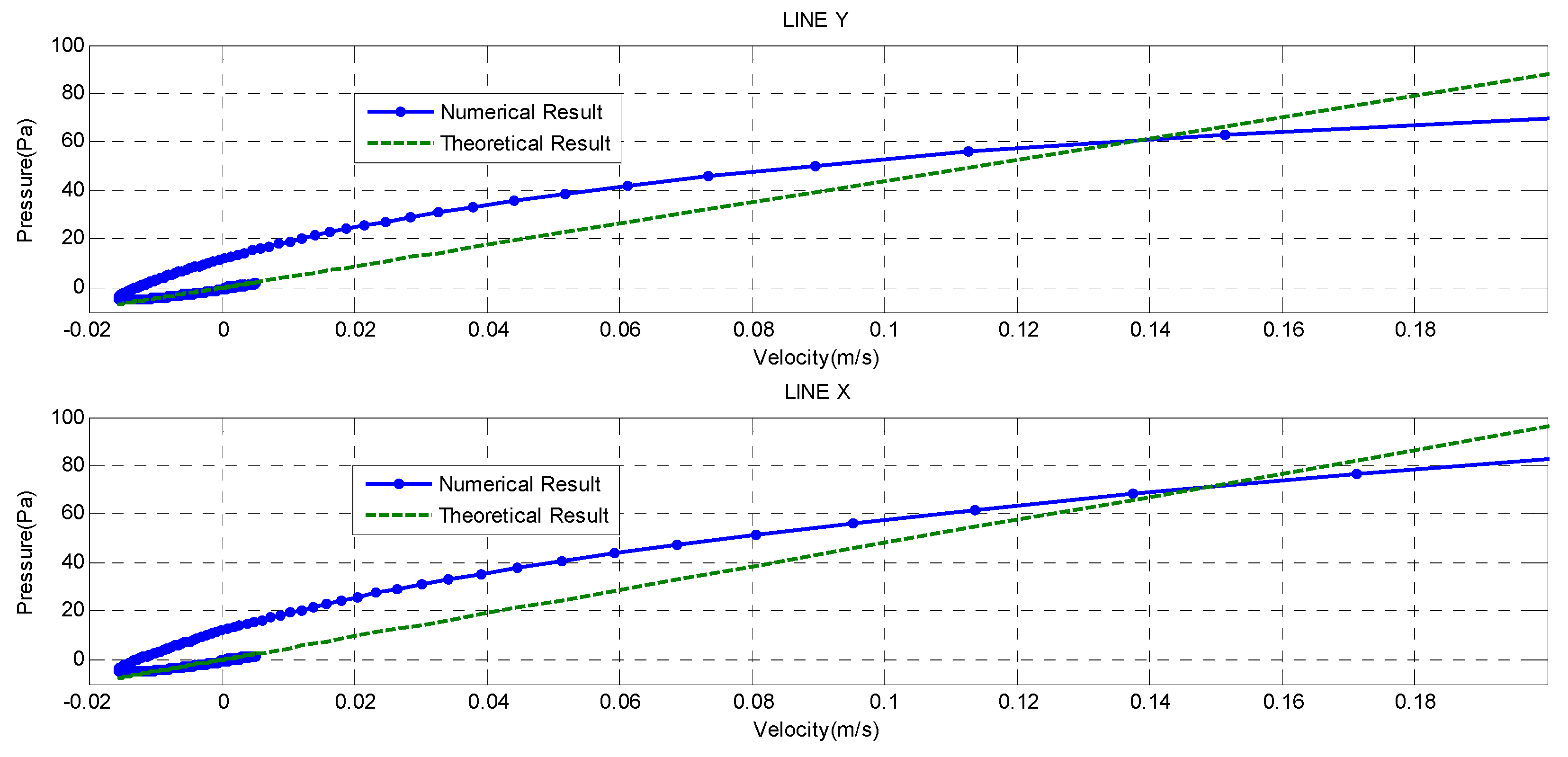
Figure 8 shows the curve of pressure versus velocity in the numerical solution and the analytical solution. The analytical solution predicts that the pressure is proportional to the velocity; the ratio is ${\rho }_{o}c$ = 417. The slope of the fitting curve is 408 with the 95% confidence bounds, which is consistent with the expected results well.

4. Parametric Analyses

To extend the applications of the analytical formulations, two more hemispherical shells rotated by the generatrix of the elliptical curve were conducted, which was inspired by the previous studies [30,31,32,33]. The length of major axis A was set to 10 m, which is the same as the conditions of hemisphere shell above, and the length of minor axis B was set to 8 m and 6 m, respectively. To compare the difference in the major axis and minor axis, the results of two lines, including X ranging from 10 m to 300 m with Y = 0, which is called LINE-X, and LINE-Y ranging from 8/6 to 300 m with X = 0, which is called LINE-Y, were investigated below.

4.1. Ellipse Geometry, A = 10, B = 8

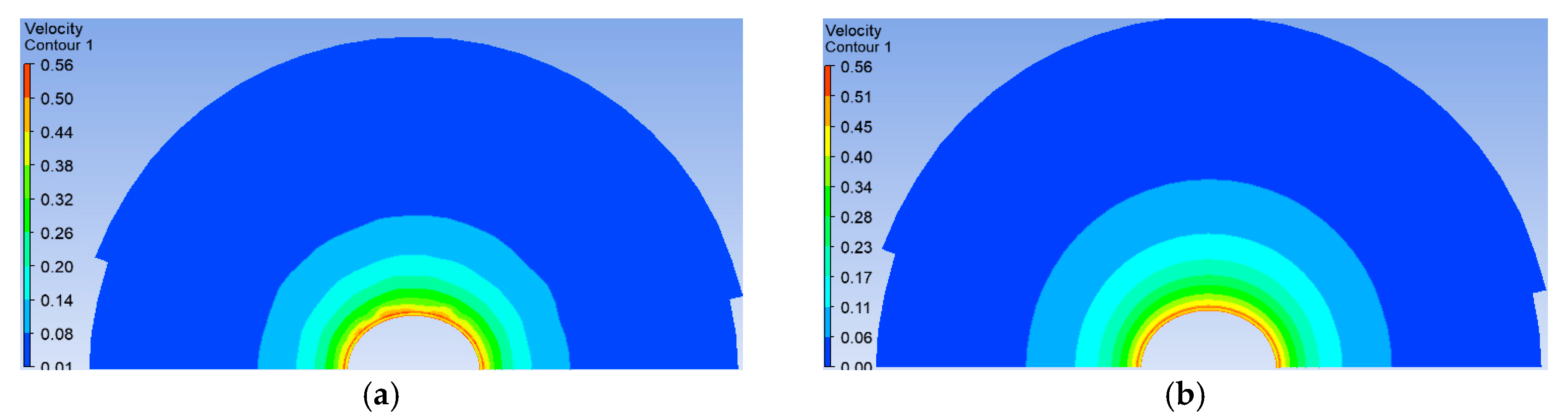
Figure 9 shows the plot of velocity versus time on the incompressible and compressible fluid condition along LINE-X and LINE-Y, respectively, when time = 1.0 s. Figure 10 presents the contour slice of velocity ranging from 10 m to 50 m, as the values of the velocity that are far from 50 m are too small to distinguish it. It is noted that there is a small deviation at about 55 m. This may be caused by the error of the numerical calculation, since the mesh size at the place far from the boundary is not small enough. It can be found that there is no evident difference regarding velocity. Also, the data is compliant with the rules that this paper presents.

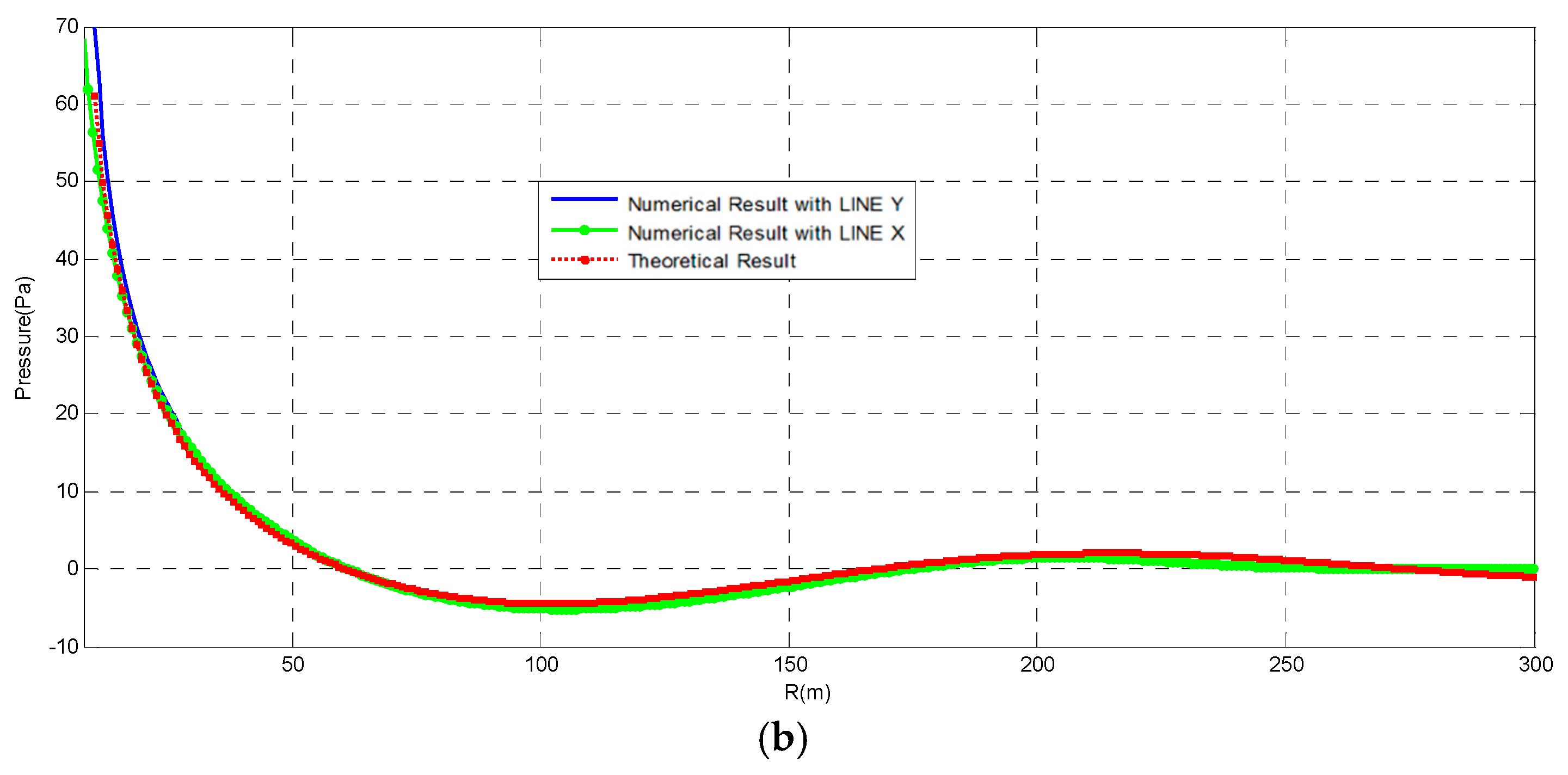
Figure 11 shows the plot of pressure versus time of the incompressible and the compressible fluid along LINE-X and LINE-Y, respectively. The results of the numerical solution and theoretical prediction agree well. In addition, Figure 12 presents the contour slice of velocity ranging from 10 m to 50 m, since the data values of the velocity that are far from 50 m are too small to be distinguished.

Figure 13 shows the curve of the pressure versus velocity in the numerical solution and the analytical solution. In this situation, the slope of the fitting curve is 427 with 95% confidence bounds, and the predicted value is 407, which is consistent with the expected results. It is noticeable that the smaller the radius, the larger the gap between the analytical and numerical result. That is because when $s$, which is linear to R, is smaller, is the approximations that are shown in Equations (33) and (15) are worse.

4.2. Elliptic Geometry A = 10, B = 6

In the situation of A = 10, B = 6, the simulation with the identical parameter is carried out. To compare with the theoretical result, the data of t = 0.65 s is shown below.

Figure 14 plots the figure of velocity versus time in incompressible and compressible fluid conditions along LINE-X and LINE-Y, respectively. To a certain degree, the flow field will be a non-uniform flow, so it can be seen from Figure 14a that there is some difference between the data values obtained from LINE-X and LINE-Y.

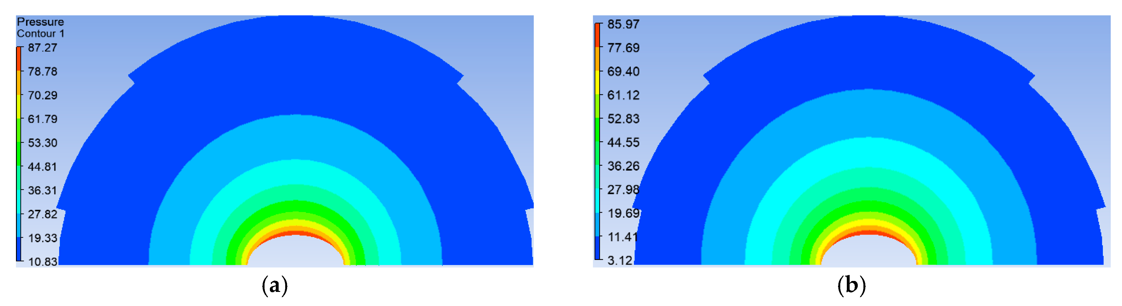
Figure 15 illustrates the contour slice of the pressure in the incompressible and compressible fluid conditions, respectively. From Figure 15, it is clear that in the middle of the shell, the velocity is larger than that of the side. Since in this situation, the slope at the side is larger than that at the middle, the fluid can distribute within the other domain close to the side boundary. In this case, the velocity of fluid decreases faster than that of the middle position.

Figure 16 presents the relationship of pressure versus time in incompressible and compressible fluid conditions along LINE-X and LINE-Y, respectively. Figure 17 depicts the contour slice of the pressure in the incompressible and compressible fluid conditions. To a certain degree, the flow will be a non-uniform flow, so it can be seen from Figure 16a that the values in LINE-X and LINE-Y are obviously different.

Figure 18 shows the relationship of pressure versus velocity and the correspondent fitting results. In the conditions of LINE-Y and LINE-X, the slope of fitting is 430 and 477, respectively. Based on the theoretical results, the slope is 417 without any change. This implies that the more irregular the shell, the larger the error between numerical and theoretical values will be. Besides, it is also found that the smaller the R, the worse the approximation will be.

5. Conclusions

A new analytical approach to calculate the pressure of the hemispherical shell vibrating in compressible fluid has been firstly developed. It is rigorously verified by the theoretical approach based on the compressible fluid assumption, which can predict the values of the velocity and pressure very well. It is found that the assumption of the compressibility of fluid plays a main role in the velocity and pressure of the FSI system. In addition, the exact solution and theoretical formulation is obtained by an integrated approach. According to the solutions, it is found that the pressure on the shell surface is proportional to the acceleration of boundary vibration when the fluid is assumed to be incompressible. Meanwhile, under the assumption of compressible fluids, the boundary pressure is proportional to the velocity of the boundary vibration. Considering the velocity of fluids, the amplitude of velocity decreases with the rate of $1/r$ in the compressible condition, whilst it decreases with the rate of $1/r^2$ in the incompressible condition.

In addition, the physical implication of the developed formula has been discussed. It is found that the motion of the boundary will propagate to the far field at the speed of sound velocity with the same frequency, but will decrease with distant r. Initially, the motion of the shell compresses the air locally, which will transfer to the far field afterward. The compression of air produces the local acceleration pressure, which is proportional to fluid velocity. The results reveal that the compression force can be exactly expressed by the new formula.

Furthermore, it can be clarified that incompressible fluid assumption for fluids can induce a large numerical error in various cases. It is also found that under the incompressible fluid assumption, the effect of air pressure is equivalent to the effect of the added mass, which confirms the scientific findings by many previous research studies and common theories that are applied today. While under the compressible fluid consideration, the effect of air pressure is equivalent to the effect of viscous damping, whose ratio is exactly ${\rho }_{o}c$. Therefore, our present findings and established formula can be used in the design and application of the resisting wind load of the spherical shell structure. The novel analytical formulation that was formed in this study can be used to predict the vibration of a spherical shell structure interacting with fluids. This new formulation can be applied to the design and analysis of the shell structure in practice.

References

- Han, Y.; Zhao, K.; Lu, Y.; Zhu, D. A method to characterize the compressibility and stability of microfiltration membrane. Desalination 2015, 365, 1–7. [Google Scholar] [CrossRef]
- Wu, X.; Ge, F.; Hong, Y. A review of recent studies on vortex-induced vibrations of long slender cylinders. J. Fluids Struct. 2012, 28, 292–308. [Google Scholar] [CrossRef]
- Tatler, B.; Macdonald, R.G. Looking at Domestic Textiles: An Eye-Tracking Experiment Analysing Influences on Viewing Behaviour at Owlpen Manor. Text. Hist. 2016, 47, 94–118. [Google Scholar] [CrossRef] [Green Version]
- Zhou, D.; Cheung, Y.K. Vibration of vertical rectangular plate in contact with water on one side. Earthq. Eng. Struct. D 2000, 2000, 693–710. [Google Scholar] [CrossRef]
- Samadi, M.; Hassanabad, M.G. Hydrodynamic response simulation of Catenary mooring in the spar truss floating platform under Caspian Sea conditions. Ocean Eng. 2017, 137, 241–246. [Google Scholar] [CrossRef]
- Tan, B.H.; Lucey, A.D.; Howell, R.M. Aero-/hydro-elastic stability of flexible panels: Prediction and control using localised spring support. J. Sound Vib. 2013, 332, 7033–7054. [Google Scholar] [CrossRef] [Green Version]
- Minami, H. Added mass of a membrane vibrating at finite amplitude. J. Fluids Struct. 1998, 12, 919–932. [Google Scholar] [CrossRef]
- Wang, J. Experiment and Analysis on Membrane Structure; Zhejiang University: Hangzhou, China, 2001. [Google Scholar]
- Yadykin, Y.; Tenetov, V.; Levin, D. The added mass of a flexible plate oscillating in a fluid. J. Fluids Struct. 2003, 2003, 115–123. [Google Scholar] [CrossRef]
- Liu, P.; Miu, W. Added Mass of Beam Vibration on Fluid with Finite Amplitude. In AER—Advances in Engineering Research; Atlantis Press: Paris, France, 2016; pp. 321–326. [Google Scholar]
- Curadelli, O.; Ambrosini, D.; Mirasso, A.; Amani, M. Resonant frequencies in an elevated spherical container partially filled with water: FEM and measurement. J. Fluids Struct. 2010, 26, 148–159. [Google Scholar] [CrossRef]
- Goodarzi, M.; Dehkordi, E.K. Complete vortex shedding suppression allocating twin rotating controllers at a suitable position. Ocean Eng. 2017, 137, 215–223. [Google Scholar] [CrossRef]
- Sorokin, S.V.; Terentiev, A.V. Flow-induced vibrations of an elastic cylindrical shell conveying a compressible fluid. J. Sound Vib. 2006, 296, 777–796. [Google Scholar] [CrossRef]
- Chen, F.; Li, Q.S.; Wu, J.R.; Fu, J.Y. Wind effects on a long span beam string roof structure Wind tunnel test field measurement and numerical analysis. J. Constr. Steel Res. 2011, 67, 1591–1604. [Google Scholar] [CrossRef]
- Stolarski, T.A. Numerical modeling and experimental verification of compressible squeeze film pressure. Tribol. Int. 2010, 43, 356–360. [Google Scholar] [CrossRef]
- Jeong, K. Hydroelastic vibration of two annular plates coupled with a bounded compressible fluid. J. Fluids Struct. 2006, 22, 1079–1096. [Google Scholar] [CrossRef]
- Jeong, K.; Kim, K. Hydroelastic vibration of a circular plate submerged in a bounded compressible fluid. J. Sound Vib. 2005, 283, 153–172. [Google Scholar] [CrossRef]
- Kubenko, V.D.; Dzyuba, V.V. Resonance phenomena in cylindrical shell with a spherical inclusion in the presence of an internal compressible liquid and an external elastic medium. J. Fluids Struct. 2006, 22, 577–594. [Google Scholar] [CrossRef]
- Eftekhari, S.A. Pressure-Based and Potential-Based Differential Quadrature Procedures for Free Vibration of Circular Plates in Contact with Fluid. Lat. Am. J. Solids Struct. 2016, 13, 610–617. [Google Scholar] [CrossRef]
- Qin, H.; Tang, W.; Hu, Z.; Guo, J. Structural response of deck structures on the green water event caused by freak waves. J. Fluids Struct. 2017, 68, 322–338. [Google Scholar] [CrossRef]
- Hu, Z.; Tang, W.; Xue, H.; Zhang, X. A SIMPLE-based monolithic implicit method for strong-coupled fluid-structure interaction problems with free surfaces. Comput. Method Appl. Mech. Eng. 2016, 299, 90–115. [Google Scholar] [CrossRef]
- Cholcz, T.P.S.; van Zuijlen, A.H.; Bijl, H. Space-mapping in fluid-structure interaction problems. Comput. Method Appl. Mech. Eng. 2014, 281, 162–183. [Google Scholar] [CrossRef]
- Evans, L.C. Partial Differential Equations, 1st ed.; Providence, R.I., Ed.; American Mathematical Society: New York, NY, USA, 1998. [Google Scholar]
- Mattheij, R.M.M.; Rienstra, S.W.; Boonkkamp, J.H.M.T. Partial Differential Equations: Modeling, Analysis, Computation; Society for Industrial and Applied Mathematic: Philadelphia, PA, USA, 2005. [Google Scholar]
- Chen, F.B.; Li, Q.S.; Fu, J.Y.; Wu, J.R. Characteristics of Wind Loads on Long-span Roof. In Applied Mechanics and Materials; Trans Tech Publications Ltd.: Zurich, Switzerland, 2012; pp. 807–812. [Google Scholar]
- Jiang, S.; Tang, P.; Zou, L.; Liu, Z. Numerical simulation of fluid resonance in a moonpool by twin rectangular hulls with various configurations and heaving amplitudes. J. Ocean Univ. China 2017, 16, 422–436. [Google Scholar] [CrossRef]
- Si, X.H.; Lu, W.X.; Chu, F.L. Modal analysis of circular plates with radial side cracks and in contact with water on one side based on the Rayleigh–Ritz method. J. Sound Vib. 2012, 331, 231–251. [Google Scholar] [CrossRef]
- Wagner, H.N.R.; Hühne, C.; Rohwer, K.; Niemann, S.; Wiedemann, M. Stimulating the realistic worst case buckling scenario of axially compressed unstiffened cylindrical composite shells. Compos. Struct. 2017, 160, 1095–1104. [Google Scholar] [CrossRef]
- Chung, M.H. Hydrodynamics of flow over a transversely oscillating circular cylinder beneath a free surface. J. Fluids Struct. 2015, 54, 27–73. [Google Scholar] [CrossRef]
- Kaewunruen, S.; Chiravatchradej, J.; Chucheepsakul, S. Nonlinear free vibrations of marine risers/pipes transporting fluid. Ocean Eng. 2005, 32, 417–440. [Google Scholar] [CrossRef]
- Remennikov, A.M.; Kaewunruen, S. Impact resistance of reinforced concrete columns: Experimental studies and design considerations, Progress in Mechanics of Structures and Materials. In Proceedings of the 19th Australasian Conference on the Mechanics of Structures and Materials, ACMSM192007, Christchurch, New Zealand, 29 November–1 December 2006; pp. 817–823. [Google Scholar]
- Liu, P.; Kaewunruen, S.; Zhao, D.; Shang, S. Investigation of the dynamic buckling of spherical shell structures due to subsea collisions. Appl. Sci. 2018, 8, 1148. [Google Scholar] [CrossRef]
- Kaewunruen, S.; Li, D.; Chen, Y.; Xiang, Z. Enhancement of dynamic damping in eco-friendly railway concrete sleepers using waste-tyre crumb rubber. Materials 2018, 11, 1169. [Google Scholar] [CrossRef] [PubMed]
- Kaewunruen, S.; Sussman, J.M.; Matsumoto, A. Grand Challenges in Transportation and Transit Systems. Front. Built Environ. 2016, 2, 4. [Google Scholar] [CrossRef]
Figure 1.
The typical hemispherical shell structure.
Figure 2.
The state of the vibration of a hemispherical shell.
Figure 3.
Spherical symmetry model of a hemispherical shell vibrating in unbounded fluid. (a) Transformation of random domain to computational domain; (b) mesh and boundary conditions.
Figure 4.
The relationship between velocity vs. radius of incompressible and compressible fluid when = 1.0 s.
Figure 5.
The contour slice of velocity of incompressible and compressible flow, t = 1.0 s, R = 50 m. (a) Incompressible flow; (b) compressible flow.
Figure 6.
The relationship between pressure vs. radii in incompressible and compressible flow when = 1.0 s.
Figure 7.
The contour slice of pressure of incompressible and compressible flow, t = 1.0 s, R = 50 m. (a) Incompressible flow; (b) compressible flow.
Figure 8.
The relationship between pressure vs. velocity in compressible flow, when t = 1.0 s.
Figure 9.
The relationship between velocity vs. time of incompressible and compressible flow, t = 1.0 s, R = 50 m. (a) Incompressible flow; (b) compressible flow.
Figure 10.
Figure 11.
The relationship between pressure vs. time of incompressible and compressible flow. (a) Incompressible flow; (b) compressible flow.
Figure 12.
Figure 13.
Velocity vs-pressure graph in compressible flow, with ellipse A = 10, B = 8.
Figure 14.
The relationship between velocity vs. time of incompressible and compressible fluid, t = 0.65 s. (a) Incompressible flow; (b) compressible flow.
Figure 15.
The contour slice of velocity of incompressible and compressible flow, t = 0.65 s, R = 50 m. (a) Incompressible flow; (b) compressible flow.
Figure 16.
The relationship between pressure vs. time of incompressible and compressible flow, t = 0.65 s, R = 50 m. (a) Incompressible flow; (b) compressible flow.
Figure 17.
The contour slice of pressure of incompressible and compressible flow, t = 0.65 s, R = 50 m. (a) Incompressible flow; (b) compressible flow.
Figure 18.
The relationship between velocity vs. pressure in compressible flow, with ellipses A = 10, B = 8.