Damage Mechanism Evaluation of Large-Scale Concrete Structures Affected by Alkali-Silica Reaction Using Acoustic Emission

Abstract

Alkali-silica reaction has caused damage to concrete structures, endangering structural serviceability and integrity. This is of concern in sensitive structures such as nuclear power plants. In this study, acoustic emission (AE) was employed as a structural health monitoring strategy in large-scale, reinforced concrete specimens affected by alkali-silica reaction with differing boundary conditions resembling the common conditions found in nuclear containments. An agglomerative hierarchical algorithm was utilized to classify the AE data based on energy-frequency based features. The AE signals were transferred into the frequency domain and the energies in several frequency bands were calculated and normalized to the total energy of signals. Principle component analysis was used to reduce feature redundancy. Then the selected principal components were considered as features in an input of the pattern recognition algorithm. The sensor located in the center of the confined specimen registered the largest portion of AE energy release, while in the unconfined specimen the energy is distributed more uniformly. This confirms the results of the volumetric strain, which shows that the expansion in the confined specimen is oriented along the thickness of the specimen.

1. Introduction

Alkali-silica reaction (ASR) is a chemical processes that has caused damage in concrete structures such as bridges [1,2,3,4], nuclear power plants [5,6,7,8,9], and concrete dams [5,10]. This reaction usually occurs between alkali hydroxides in the pore solution and the reactive silica in some aggregates. The result is an alkali-silica gel, which is hygroscopic and imbibes water and humidity. The gel expands in humidity exceeding 80% [6]. This expansion induces pressure on the concrete matrix and aggregates and causes micro-cracks and cracks when the pressure exceeds the tensile strength of the concrete [11,12]. Several traditional methods such as visual inspection, coring, and petrographic analysis have been utilized for monitoring and identifying the behavior of damage caused by ASR. Visual inspection is very subjective and depends on experience [13]. In addition, damage can only be detected by using this method, once it has reached the surface. Coring is a destructive method, which is discouraged in sensitive structures like nuclear power plants. Moreover, it is difficult to generalize the global condition of structures through evaluation of a few cores. Petrographic analysis is also mostly dependent on the experience of the examiner, is likewise a destructive method, and is costly and time-consuming. Linking the micro-state of the material examined to the condition of the entire structure using petrographic analysis is difficult [11], although this is an active research area (RILEM TC-259). Therefore, to monitor structures affected by ASR, non-destructive and global/semi-global methods are attractive. Acoustic emission (AE) is a health monitoring approach which acts as a passive receiver to record internal activities in structures. This method is capable of continuous monitoring which is not the case with most traditional methods. In addition, AE sensors are very sensitive and can capture signals due to micro-scale defect formations coming from the internal regions of structures rather than only those at the surface [14,15]. Several studies have been conducted to evaluate the use of AE in detecting the damage in concrete caused by ASR in the laboratory [11,16,17,18,19].

Lokajíček et al. [16] employed ultrasonic sounding and AE to monitor the microstructural changes in mortar bars with different levels of aggregate reactivity. The P-wave velocity increased in the first days of the experiments and then declined abruptly for the specimens with the reactive aggregates. Furthermore, AE cumulative energy indicated the clear difference between the specimens with the reactive aggregates compared to the specimens without any ASR reactivity. Farnam et al. [17] characterized the AE signature for crack formations in aggregates, cement matrix, and interfacial transition zones (ITZ) during alkali-silica reaction using peak frequency and frequency of centroid of the AE signals. The high-frequency signals were assigned to the crack formation in the aggregate, while low-frequency signals were attributed to the crack formation in ITZ and cement matrix. Abdelrahman et al. [11], conducted an accelerated ASR test on concrete prism specimens. A correlation between cumulative signal strength and length change of the prism specimens was identified, and an AE based intensity analysis chart for the classification of ASR damage conditions in correlation with petrographic damage rating indices was developed.

All previously mentioned, research has been focused on ASR-induced damage detection using AE data in small-scale specimens (laboratory scale), which is far from the conditions found in real structures in the field. Furthermore, the stress boundary condition has generally not been taken into consideration in previous studies, while the stress boundary condition has proven to have a large effect on damage distribution in concrete structures affected by ASR [20,21].

In this study, acoustic emission is utilized to monitor the effects of ASR on large-scale, reinforced concrete structures while considering stress induced boundary conditions in completely plane-confined and partially plane-confined specimens. There are several differences between damage detection of small-scale and large scale structures using acoustic emission. The main challenge with monitoring of small-scale structures using AE is reflections. An example of an ASR study using AE on small-scale specimens was conducted by Abdelrahman et al. [11]. For large-scale structures, attenuation and dispersion of waves are of primary concern. Many sensors with an appropriate layout are needed for damage detection and source localization.

The test specimens were assembled, cured, and monitored at the University of Tennessee, Knoxville, and are part of a test program sponsored by the US DOE Light Water Reactor Sustainability Program. The confined specimen has a complete confinement provided by a rigid steel frame and steel reinforcement meshes. The unconfined specimen has partial confinement provided by steel reinforcement meshes. The specimens without transverse reinforcement resemble construction reminiscent of nuclear power plant containments. An unsupervised pattern recognition algorithm was employed to classify the AE signals based on frequency-energy based features. Different damage mechanisms for the confined and unconfined specimens were identified using AE data.

2. Materials and Test Setup

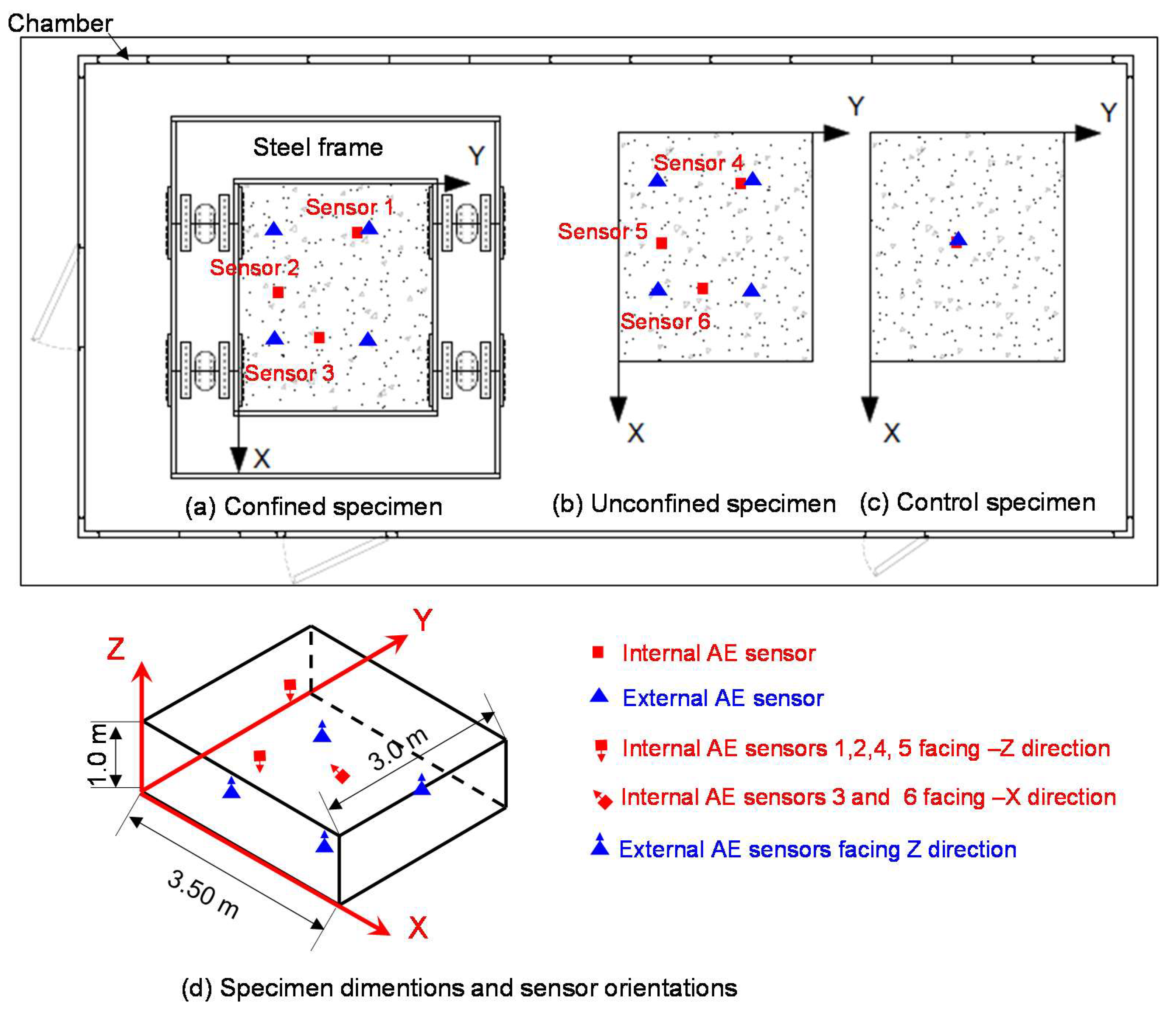
2.1. Specimen and Chamber Preparation

In this study, three large-scale reinforced concrete blocks were cast. Two specimens were reactive and one was a control specimen (Figure 1). Reactive specimens are the specimens that experience expansion due to alkali-silica reaction. Two layers of steel reinforcement mesh were located at the top and bottom surfaces of the specimens. The reinforcement mesh includes US #11 Grade 60 with a nominal diameter of 36 mm (1.41 inches) at 25 cm (10 inches) spacing (Figure 2). The specimens have 7.62 cm (3 inches) cover at top and bottom of the specimens. Moreover, the square steel plates were installed on the ends of the rebar to achieve the full development length in a relatively short distance inside the specimens. For concrete mixture, 350 kg/m³ cement, 175 kg/m³ water, 1180 kg/m³ coarse aggregate, and 728 kg/m³ fine aggregate were used for both reactive and control specimens. The main difference between the specimens was using of NaOH or LiNO₃. In the reactive specimens, 9.8 kg/m³ NaOH solution was added, while in the control specimen 1.9 kg/m³ LiNO₃ was included in the mixture [22].

The coarse aggregates in both control and reactive specimens were greenschist coarse aggregates from North Carolina, which were highly-reactive. Non-reactive manufactured sand and low-alkali Portland cement Type II were also utilized in the concrete mixture. Water to cement weight ratio for both control and reactive specimens was 50%. To increase the alkali content of reactive specimens, 50% sodium hydroxide solution was added to the mixture for reactive specimens. Additionally, a 30% lithium nitrate solution was added to the control specimens to mitigate the ASR effect. More details regarding concrete mixture design was presented by Hayes et al. [22].

The specimens shown in Figure 1 have a cubic shape with dimensions of 3.50 m × 3.0 m × 1.0 m (136 inch × 116 inch × 40 inch). There are two reactive specimens; confined and unconfined specimens. A rigid steel brace was utilized to restrain the confined specimen from expanding in the lateral plane. The unconfined specimen does not have a steel brace in its plane. The two reactive specimens resemble the different stress boundary conditions found in real structures. A 1.5 mm layer of polyethylene was employed between the concrete and the steel frame in the confined specimen to reduce friction. More detailed information about the specimens and steel frame design were presented in Hayes, et al. [22]. In this experiment, the specimens stand on four short, steel columns (76 cm height) to provide access to the bottom of the specimens.

Each specimen’s formwork was removed 12 days after casting which gave them time for final finishing and concrete setting. After casting, the specimen surfaces were sprayed with curing compound and covered with wet burlap and plastic sheets to reduce moisture loss and cracks from shrinkage during drying. The burlap was kept wet until chamber construction was complete [22].

A large chamber with the dimensions of 16.2 m long, 7.3 m wide, and 3.7 m high was constructed around the specimens to control the temperature and relative humidity of the environment. The chamber was equipped with systems that kept the specimens at the environmental temperature of 38 ± 1 °C and humidity of 95% ± 5%. The environmental chamber was initiated 26 days after casting and operated continuously except for shutdown for measurements and inspections [22].

2.2. Measurement Equipment

To measure the strain inside the specimens, two kinds of strain sensors, alkali-tolerant strain transducers (KM-100B from Tokyo Sokki Kenkyujo) and long-gauge fiber optic extensometers (from SMARTECH/Roctest), were employed. In total, sixty-four 100 mm-gauge strain transducers were placed inside the specimens, along with the specimen dimensions. The sensors were fixed on the support fabricated by smooth steel bars with a diameter of 3 mm. Additionally, five high-precision, fiber optic extensometers were installed inside the specimens. The sensors in the X-Y plane had 1.5 m and 1.8 m gauge lengths and were located at the bottom of the specimens. Two fiber optic sensors were installed along the specimen thickness with a gauge length of 0.8 m [22].

Seven acoustic emission sensors were utilized in each of the confined and unconfined specimens (reactive specimens) as shown in Figure 1 and Figure 2. Two sensors were employed for the control specimen. The internal AE sensors were broadband WDIUC-AST (manufactured by MISTRAS Group, Inc., Princeton Junction, NJ, USA), with an operating frequency range of 200–900 kHz and an internal low-noise 40 dB preamplifier. The external sensors were resonant R6I-UC (manufactured by MISTRAS Group, Inc., Princeton Junction, NJ, USA), with an operating frequency range of 35–100 kHz and an internal 40 dB preamplifier. The special polymer coating on the sensors (internal and external) with an internal waterproof cable makes the sensors insulated, non-conductive, and capable of operating under water.

Three broadband sensors were installed inside the reinforcement cages prior to casting for reactive specimens and one sensor was installed in the control specimen. Sensors 1, 2, 4, and 5 were attached under the second layer of top reinforcement mesh (under reinforcement in the Y direction) with epoxy and fastened to the rebar by several cable ties and duct tape, with the sensing surface facing downward along the negative Z axis (Figure 1d and Figure 2d). Sensors 3 and 6 were in the middle of the specimen thickness, with the sensing surface facing toward the negative X axis (Figure 1d). Sensors 3 and 6 were attached on the supports by epoxy and duct tape and cables were fastened on the support by cable ties (Figure 2c). The supports were fastened to the top and bottom reinforcement meshes. The locations of internal sensors were colored on the top reinforcements to avoid over-vibrating during casting and potentially decoupling the sensors.

Four resonant sensors were attached at the bottom of the reactive specimens and one to the control specimen (Figure 2b). The resonant sensors were attached with epoxy on the surface of the concrete and fixed by holders as shown in Figure 2b. Internal and external sensors are referred to as broadband and resonant sensors, respectively, in this paper. The holders were made of stainless steel and polyurethane pads were attached between the concrete and the holders to avoid potential corrosion in the holders.

External and internal sensors pose differing technical challenges. Internal sensors are of scientific interest and are not well-suited for implementation in existing structures. One potential technical consideration is the formation of voids around the sensors due to concrete shrinkage. This may result in interruption of data or reduction of sensitivity. Another technical challenge is lack of access after casting. The external sensors are accessible, but decoupling may be a consideration.

A 16-channel Sensor Highway II (SHII), manufactured by MISTRAS Group, Inc. (Princeton Junction, NJ, USA), was utilized as a data acquisition system. The sensitivity of external sensors was checked by applying Hsu-Nielsen sources [23].

The sampling rate was set to 1000 kHz. Pre-trigger time is the period required for data acquisition to save a signal prior to threshold intersection, which was set to 256 µs. HDT (hit definition time) is the time for which if a signal crosses the threshold the signal will continue until the end of HDT without stopping. HDT was set to 400 µs. HLT (hit lockout time) is the time defined at the end of a signal for neglecting any reflected signal that exceeds the threshold, which was set to 200 µs. PDT (peak definition time) is the time which ensures correct identification of the signal peak for rise time and peak amplitude measurements [24]. In this study, PDT was set to 200 µs. The initial threshold was 32 dB.

3. Analysis Method

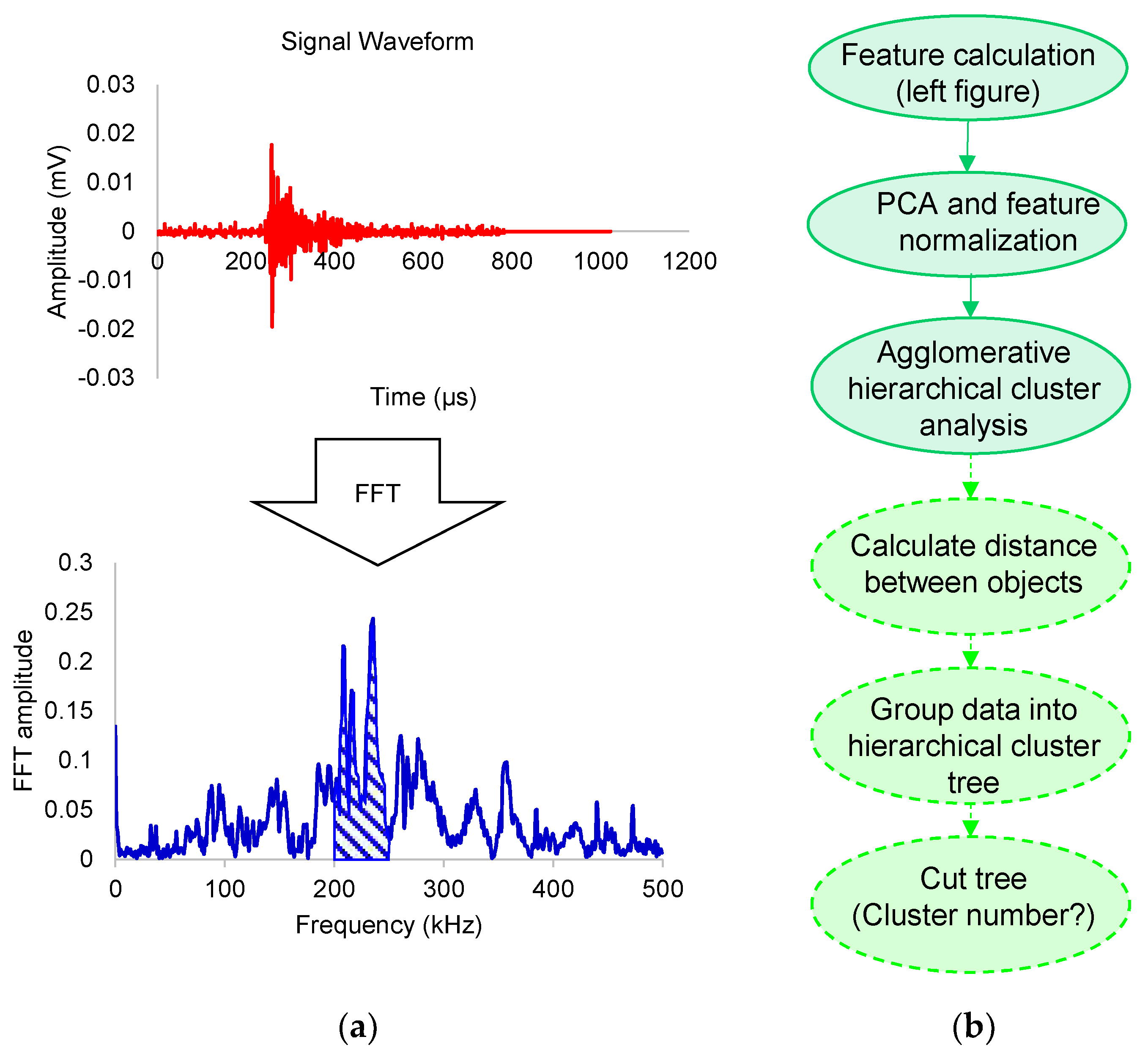
3.1. Pattern Recognition Algorithm

To identify the damage mechanisms in the reactive specimens a pattern recognition algorithm was employed for data classification. Pattern recognition is under the machine learning field and has two major types: unsupervised and supervised. When a background history for a data set is available or the data set has labeled classes, supervised pattern recognition is employed. If there are no labeled classes available, unsupervised pattern recognition can be utilized to identify the potential patterns in the data set based on the selected features.

An agglomerative hierarchical clustering algorithm [25] was employed for classifying the AE data into subsets. The clustering procedure is chronologically illustrated in Figure 3. The first step in the pattern recognition was deriving the frequency-based features for the signals. AE signals were transferred into the frequency domain using the Fast Fourier Transform (FFT). The FFT amplitude spectra were determined for each AE signal and the frequency domain was divided into ten frequency ranges. Then, signal energy in each frequency range was calculated and normalized to the total energy of the signal. These ten signal energies are the signal features. For example, in Figure 3a, the area of the hatched region is the energy of the signal in the frequency band from 200 kHz to 250 kHz. This value is normalized to the total energy of the signal, which is the entire area under the FFT spectrum. Principle component analysis (PCA) was used to reduce redundancy in the data. In this analysis, the original data is projected to the new orthogonal coordinates having high variation. An input for PCA is a matrix with the number of columns and rows equal to the feature numbers and the number of hits. Then a variance-covariance matrix for the features was calculated. The coefficients and variance of a specific principle component were calculated by eigenvalue analysis of the variance-covariance matrix. The principal components were selected in a way that represented more than 90% of the entire data. The principal components of the original features were selected as the input features for the pattern recognition algorithm. The algorithm initially calculated the Euclidian distance between the resulting data from PCA analysis. The result was a proximity matrix that contained distances between the original objects (data).

The objects were initially linked together according to calculated distances in the previous step and Ward’s method. Ward’s method is based on calculating the total within-cluster sum of squares of the data resulting from combining the clusters [25]. In each level, the data was merged into a binary linkage and the clusters were again merged into new clusters according to the Ward’s method. This procedure was continued to form a single cluster which includes all data. The number of the cluster was determined according to the developed dendrogram and the height of each link with respect to the adjacent links [26].

4. Results and Discussions

The internal strains of the specimens in X, Y, and Z directions were recorded from the casting date. The results are presented up to 200 days in Figure 4. The data is presented from 51 days in the figures since external sensors were attached in this day and all the figures in this paper remain in a same time scale for a convenient comparison. Figure 4a shows the average expansion along the specimen dimensions for the reactive specimens and the average volumetric expansions for both reactive and control specimens are presented in Figure 4b. The results for volumetric strains show that reactive specimens were expanded. Conversely, the control specimens had no expansion and the internal strain was relatively constant, only showing small shrinkage over time. However, the volumetric strains for both confined and unconfined specimens were very close. This observation indicates that an imposed confinement in the specimens did not influence the expansion of the entire specimens (volumetric strain). Furthermore, the confinement changed the direction of expansion (Figure 4a).

Generally, the expansion through the thickness of the reactive specimens (Z direction) is much larger than the expansion throughout the X-Y plane, due to partial or complete confinement in the plane and lack of steel reinforcement through the thickness. The maximum strains in the Z direction for confined and unconfined specimens are approximately 3.6 and 2.1 times the strain in the Y direction, respectively, at 200 days. The steel frame in the confined specimen causes a reduction of both in-plane strains. In the confined specimen, the strain along the X direction is less than the Y direction, while in the unconfined specimen, the strain along X and Y are almost the same. The strain along the X direction in the confined specimen is 58% of the strain along the X direction in the unconfined specimen at 200 days. However, the strain along the Y direction in the confined specimen is 84% of the strain along the Y direction in the unconfined specimen at 200 days. Moreover, the confinement in X-Y plane for the confined specimen caused an increased strain rate along the Z direction (thickness). The expansion strain rate in terms of time decreases at the point around 150 days, which is named inflection point as seen in Figure 4. The inflection point in volumetric strain is considered as one of the important point for ASR modeling, where the curvature of volumetric strain is changed [27,28]. The latency and characteristic times (two modeling parameters) are experimentally determined by knowing the location of inflection point [6,28]. The inflection point is shown in Figure 4b and marked in other figures in this paper.

Acoustic emission data was recorded through the internal sensors from the casting day and resonant sensors started recording from the concrete age of 51 days. Filtering AE data is an important step for reducing the amount of non-relevant data for post-processing. The possible sources of false AE data can be friction between the structural components, such as the steel frame and specimens, and water dripping from the chamber ceiling due to high humidity. Two different filtering procedures were developed to minimize the non-genuine data for the internal and external sensors, separately. The filtering is different for the internal and external sensors due to their differences in sensitivity and location. For instance, the internal sensors are much less sensitive than the external sensors and were located inside the specimens, thereby receiving less environmental noise. The AE data below 32 dB and 41 dB for the internal and external sensors was filtered from the data set. Then, the signals were further filtered using a Swansong filtering procedure [29,30]. This method is based on the observation that genuine AE signals with high amplitude should have long duration and vice versa [11]. Therefore, false signals in this method are categorized by long duration with low amplitude and short duration with high amplitude. The data is presented in terms of duration versus amplitude distribution. Signals which did not comply with the characteristics of genuine signals were deleted based on visual observation of the waveforms. The rejection limits for the internal and external sensors are presented in

Table 1. Duration-amplitude rejection limits.

External Sensor		Internal Sensor
Amplitude (dB)	Duration (µs)	Amplitude (dB)	Duration (µs)
41–43	400<	32–35	155<
44–45	500<	36–42	260<
46–47	600<	43–100	330<
48–49	650<	-	-
50–53	820<	-	-
54–56	940<	-	-
57–65	1080<	-	-
66–100	1400<	-	-

. In addition, suspicious signals were removed by inspection of waveforms and the chamber activity timetable provided by the University of Tennessee, Knoxville. The filtered AE data from 50 to 195 days after casting for all sensors is presented in Figure 5. The figure illustrates the amplitude and cumulative signal strength (CSS) in terms of specimen age. The time window of 50 to 195 days was selected because the highest strain change rate occurred during this period. The gap in the data from 65 to 100 days is missing data due to a difficulty with the data acquisition system caused by an unexpected energy surge. The amount of data in the control specimen is much lower than the data for the reactive specimens. The difference between AE data for the control and reactive specimens is also observable from plots of cumulative signal strength versus time (Figure 5). Therefore, the relatively high AE activity for the reactive specimens can likely be associated with expansion caused by the alkali-silica reaction.

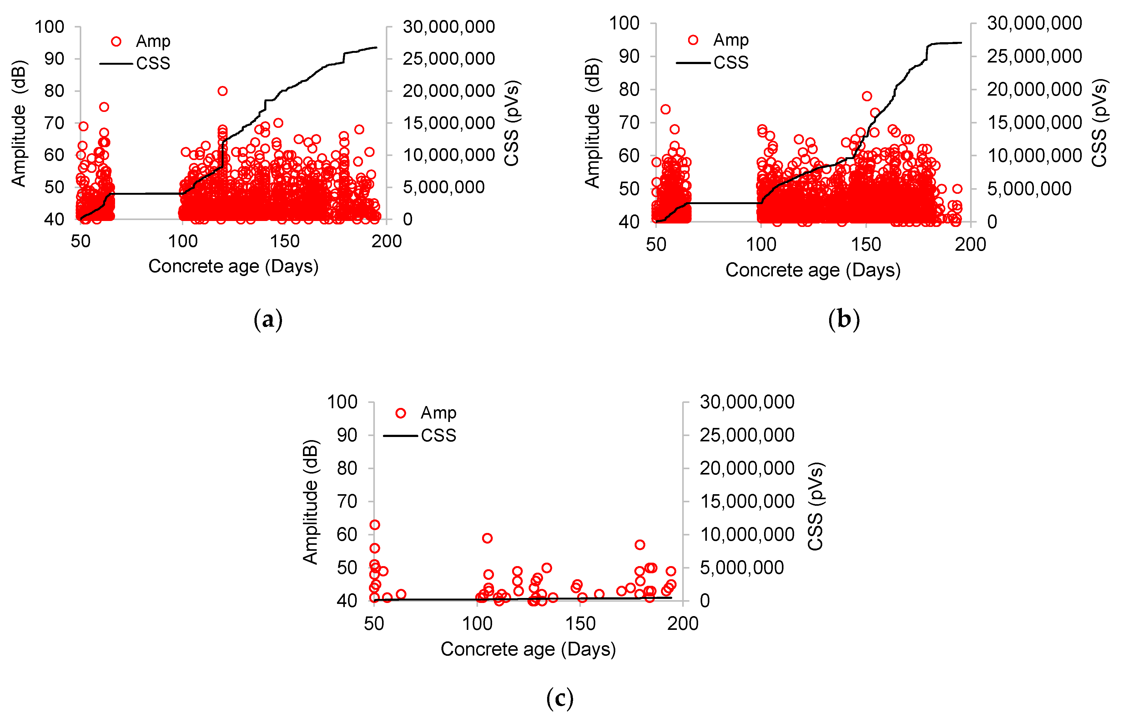
4.1. Acoustic Emission Energy Release

To enable comparisons between the confined and unconfined specimens only AE data recorded by the internal sensors is discussed. These sensors are less sensitive than the resonant sensors, which results in lower volumes of data. The main reason for choosing the broadband sensors is that their broad frequency response makes them suitable for frequency analysis. The resonant sensors attached on the bottom surface of the specimens are more representative of what may be used in practice for optimized detection and source location. Three dimensional source location of large-scale specimens requires a method to accurately calculate time of arrival for very weak signals, which is a future step of this research. This study involves frequency analysis and therefore focuses on broad band sensors. Analysis of the resonant sensor data is a future consideration.

In Figure 1, the red marks and corresponding labels in red font denotes the schematic sensor locations for both confined and unconfined specimens. Sensor coordinates are presented in

Table 2. Sensor coordinates.

Sensor No.	X (m)	Y (m)	Z (m)	$\overrightarrow{\mathit{n}}$
Sensor 1	1.08	1.91	0.86	(0,0,−1)
Sensor 2	1.85	0.78	0.86	(0,0,−1)
Sensor 3	2.34	1.46	0.5	(−1,0,0)
Sensor 4	1.1	1.59	0.86	(0,0,−1)
Sensor 5	1.83	0.88	0.86	(0,0,−1)
Sensor 6	2.36	1.59	0.5	(−1,0,0)

. The last column of the table represents the coordinates of normal vectors, which are perpendicular to the sensing surfaces of sensors and the directions of vectors are toward the outside of the sensors. The orientation of sensors is shown in Figure 1d.

The AE cumulative signal strengths of the internal sensors for the reactive specimens are presented in Figure 6a,b. The total CSS versus time for the confined specimen is much higher than the CSS for the unconfined specimen at 195 days (the CSS for the confined specimen is 2.35 times the value for the unconfined specimen). Moreover, in Figure 5a,c, it can be seen that a significant portion of released AE energy is attributed to sensor 3, which is located at mid-height of the confined specimen. The CSS rate for sensor 3 (5805 pVs/Day) is much larger than for sensors 1 and 2 (1545 and 1212 pVs/Day), thereby increasing the difference in the CSS between the sensors. On the other hand, this trend in the confined specimen is not observed in the unconfined specimen where AE energy release is not concentrated in one specific sensor. The distribution of energy was approximately uniform among the sensors. However, the CSS for the sensors at the top reinforcement mesh (sensors 4 and 5) is larger than in sensor 6.

These observations illustrate that the confined specimen has larger AE energy release in the middle layers of the specimen, which is increasing with the progression of the ASR reaction, than the unconfined specimen. This may be due to a larger expansion strain through the thickness of the confined specimen. This large expansion is expected to cause more damage through the thickness of specimen and consequently more AE energy release at middle of the thickness. In the unconfined specimen the crack distribution is expected to be less anisotropic than in the confined specimen. Therefore, it is expected that the AE energy was more uniformly distributed through the thickness of this specimen.

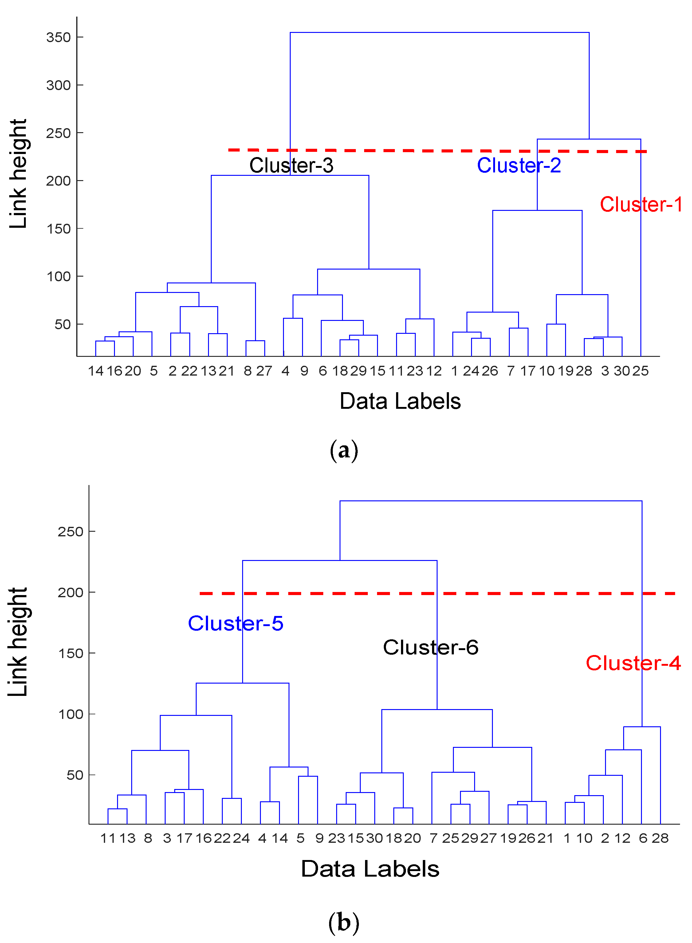
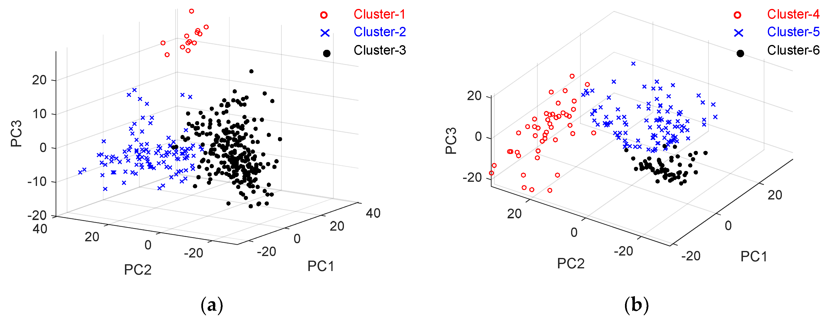
4.2. Pattern Recognition of AE Data

The AE signals were classified according to the agglomerative hierarchical algorithm as explained in Section 3.1. Dendrograms resulting from the analysis are presented in Figure 7. Dashed red lines in the subfigures indicate the desired height of links for clustering. The results of the pattern recognition show three clusters for each reactive specimen (both confined and unconfined). The clusters of confined specimens are indicated by Cluster-1, Cluster-2, and Cluster-3. Accordingly, the clusters of the unconfined specimen are labeled Cluster-4, Cluster-5, and Cluster-6. The horizontal axis in Figure 7 gives the data labels, which show either labels of the original data sets (signal number) or the label number of the clusters that resulted from merging the original data. The height of each link shows the distance between the two objects. Each link between two objects is shown by an upside-down U-shaped line in the figure. The data is shown in terms of the first three principal components (PC) to visualize the distribution of clusters with respect to each other in Figure 8. Although some signals in the cluster 5 and 6 were not ideally separated, in general, the clusters indicate a reasonable separation in the PC space (Figure 8). The reason for an overlap between clusters 5 and 6 is that some signals in cluster 5 have a similar energy contribution in a specific frequency range to some signals in cluster 6. As seen in Figure 9b, clusters 5 and 6 have similar average energy contribution between 250 to 300 kHz.

The average energy of signals in terms of frequency ranges is shown in Figure 9 for the reactive specimens. These values, as previously mentioned, were calculated using the FFT amplitude spectrum. Afterward, the calculated values were normalized by the total energy of the signal. The average values for each cluster were then calculated. The energy shift to the higher frequency components for the unconfined specimen is apparent when viewed alongside the confined specimen. The clusters in each specimen can be separated based on the frequency content. In the confined specimen, the low-frequency cluster (Cluster-1) has approximately 69% of its energy in a frequency range of 0–100 kHz. The medium-frequency cluster (Cluster-2) has 42% of its energy concentrated in a frequency range of 50–150, while the high-frequency cluster (Cluster-3) has 51% of its energy between 150–300 kHz.

In the unconfined specimen, the low-frequency cluster (Cluster-4) has 62% of its energy in a frequency range of 0–150 kHz and the medium-frequency cluster (Cluster-5) has 49% of its signal energy in the frequency range of 150–300 kHz. The high-frequency cluster (Cluster-6) has 54% of its signal energy concentrated between the frequencies of 300–450 kHz. The Cluster-3 and Cluster-5 share similar frequency content. More signal features for the clusters are illustrated in Figure 10. The average feature values for each cluster were normalized by the maximum feature values for each cluster. In the confined specimen, Cluster-1 initiated at a higher concrete age (data was analyzed through a concrete age of 195 days) than clusters with higher frequencies (Cluster-2 and Cluster-3). The average amplitude of the signals in Cluster-3 (the highest frequency) is higher than the other signals. Average signal strength for Cluster-1 is lower than the values for Cluster-2 and Cluster-3, and duration is higher for the cluster with the lowest frequency content, for example, Cluster-1.

A clear correlation is present between the frequency content of the signal clusters and the rise angle values (rise time over amplitude ratio) as has been observed by other researchers [31,32]. The higher the frequency components are in a signal, the lower rise angle value the signal possesses. In the unconfined specimen, Cluster-5 and Cluster-6 exhibit higher hit rates at the higher concrete age compared to Cluster-4, and the average amplitude of signals for the clusters with higher frequency components is slightly higher than for signals in Cluster-4. However, the average duration for the signals in the cluster with the low-frequency components (Cluster-4) is much longer than the duration for Cluster-5 and Cluster-6.

In Figure 11, the variation of cumulative signal strength in terms of the age of the concrete for each cluster is presented. The cumulative signal strengths were normalized by the maximum value for each specimen. In the confined specimen, the signals with the highest frequency components (Cluster-3) have dominant CSS from the early age. However, the CSS of Cluster-2 is very close to the CSS of Cluster-3 up to the concrete age of 150 days. After 150 days, the CSS rate for Cluster-3 increases, while the CSS rate of Cluster-2 continues with approximately the same rate. The signals in cluster Cluster-1 have negligible signal strength compared to Cluster-2 and Cluster-3 and initiate primarily after 120 days. In the unconfined specimen, the AE energy is primarily attributed to cluster Cluster-4 up to approximately 150 days. After 150 days, the clusters with the higher frequency components (Cluster-5 and Cluster-6) become prominent in terms of AE energy release.

The distribution of total AE signal strength for the classified clusters and sensors at different ages of the concrete (66, 150, 195 days) are illustrated in Figure 12. These distributions are referred to as signal strength contribution factors (SSCF). The 66th day and 195th day were selected to illustrate the trend of data at the beginning and end of the evaluated time window. The 150th day was selected because in both reactive specimens there was an obvious change in the rate of CSS of the clusters with high-frequency components in comparison to the lower frequency components. The figures on the left show results of the confined specimen and the figures to the right show data from the unconfined specimen.

In the confined specimen, most of the energy contribution is related to Cluster-2 (energy concentration in 50–150 kHz) and Cluster-3 (energy concentration in 150–300 kHz). The SSCF for Cluster-3 is increases with time, particularly after 150 days. Most of the AE energy for Cluster-3 is concentrated in sensor 3 (mid-thickness of the specimen) after 100 days. Cluster-2 and Cluster-3 both have prominent AE energy at sensor 2 before the 66th day. Then the highest AE energy portion moves to sensor 3, whereas SSCF of Cluster-2 is much lower than Cluster-3, especially after 150 days. The SSCF for cluster Cluster-1 is negligible compared to other clusters. In the unconfined specimen, the highest SSCF is for cluster Cluster-4 (energy concentration between 0–150 kHz) at sensor 4 (attached to top reinforcement) at 66 days. However, this energy contribution decreases with time, and the SSCF of the clusters with high-frequency components (Cluster-5 and Cluster-6) increases with time. There is no obvious energy concentration in the sensor located at mid-thickness of the specimen (sensor 6), which is different from what is observed in the confined specimen. In both specimens, the SSCF declines in low-frequency signals and increases in high-frequency signals with time. This trend in signal frequency from low to high in the confined specimen is not pronounced before 150 days. The SSCF for cluster Cluster-3 is slightly greater than the Cluster-2 at 150 days. The signal frequency trend initiates primarily after 150 days in this specimen. On the other hand, in the unconfined specimen, the frequency content evolution of AE signals is obvious from an earlier stage of ASR reaction (66 days) and is more significant after 150 days.

The confined specimen has a higher extensional strain along the Z direction than the unconfined specimen (approximately 42% more at 195 days). This expansion leads to tension concentration through the thickness of the confined specimen. Since there is no confinement through the specimen thickness it is susceptible to crack formation. In the unconfined specimen, the expansion strain is more evenly distributed between the X-Y plane and the thickness. Therefore, the tension is more uniformly distributed in the entire specimen in comparison to the confined specimen. This is also observable from the AE data, where sensor 3, located at the mid-height of the confined specimen, has a larger SSCF than the unconfined specimen (e.g., 65% for the confined specimen versus 35% for the unconfined specimen at 195 days).

As mentioned previously, the frequency of AE signals progresses from low to high as the concrete ages. This may be attributable to the formation of cracking through the coarse aggregate due to ASR progression. The crack formation inside the aggregate is expected to have higher frequency components than the cement matrix and interfacial transition zone (ITZ) as mentioned by Farnam et al. [17]. The transition from low-frequency signals to the high-frequency signals in the confined specimen initiated later than for the unconfined specimen (after 150 days). However, there are different contradictory hypotheses relating to formation of cracks in concrete due to ASR [33]. For instance, osmotic pressure theory was proposed by Hanson to describe the mechanism of expansion [34]. In this theory, the cement paste surrounding to reactive aggregates acts as a semi-permeable membrane, which water solution can pass inside the region around the reactive aggregates, but alkali-silica ions are enclosed in the reactive regions. This causes osmotic pressure and alkali-silica gel swells and exerts pressure to the cement paste. This pressure leads to crack formation in the cement paste [34]. McGowan and Vivian also proposed a similar theory as osmotic theory, which transforming a solid alkali-silica layer on a reactive aggregate to a gel by absorbing moisture from the pore solution was explained as a main reason of cracking in the cement paste due to ASR [35]. Bazant and Steffens suggested that the cracking is caused in the cement paste and interfacial transition zone due to accumulation of alkali-silica gel in the interfacial transition zone and resulting gel pressure [36]. On the other hand, Dron and Brivot assumed that crack formation occurred far away from reactive aggregates due to diffusing dissolved silica away from aggregate into the pores in the cement paste [37]. Some researchers observed that ASR gel initially forms inside a reactive aggregate and causes the pressure and crack formation inside the aggregate and surrounding cement paste [12,38,39,40,41]. Ponce and Batic [42] related the cracking pattern of concrete due to ASR to the types of reactive aggregate. ASR cracks start to form inside aggregate or in the cement matrix depending on the aggregate type [42].

In the confined specimen, the CSS rate of Cluster-3 (energy concentration 150–300 kHz), started to increase at the age of 150 days. In the unconfined specimen, the CSS rate for the cluster with the higher frequency components also increases around that time. 150 days is close to the inflection point of the volumetric strain curve, after which point expansion rates decrease. In addition, the first visible cracks were observed at the age of 150 days on the sides of the unconfined specimen, but no cracks were visible on the top surface of the unconfined specimen. Cracks could not be traced in the confined specimen on the sides due to the steel confinement frame. From the above observations, 150 days is a significant time period for ASR in the specimens, which generally agrees with trends in the AE data.

5. Conclusions

Acoustic emission was utilized for monitoring the activities caused by ASR in large-scale reinforced concrete specimens. The specimens resemble common nuclear power plant containments with no shear reinforcement. An agglomerative hierarchical algorithm was used to classify the AE data based on the energy-frequency dependent features to study and identify the damage mechanisms in the specimens with different stress boundary conditions. The conclusions of this study are summarized as follows:

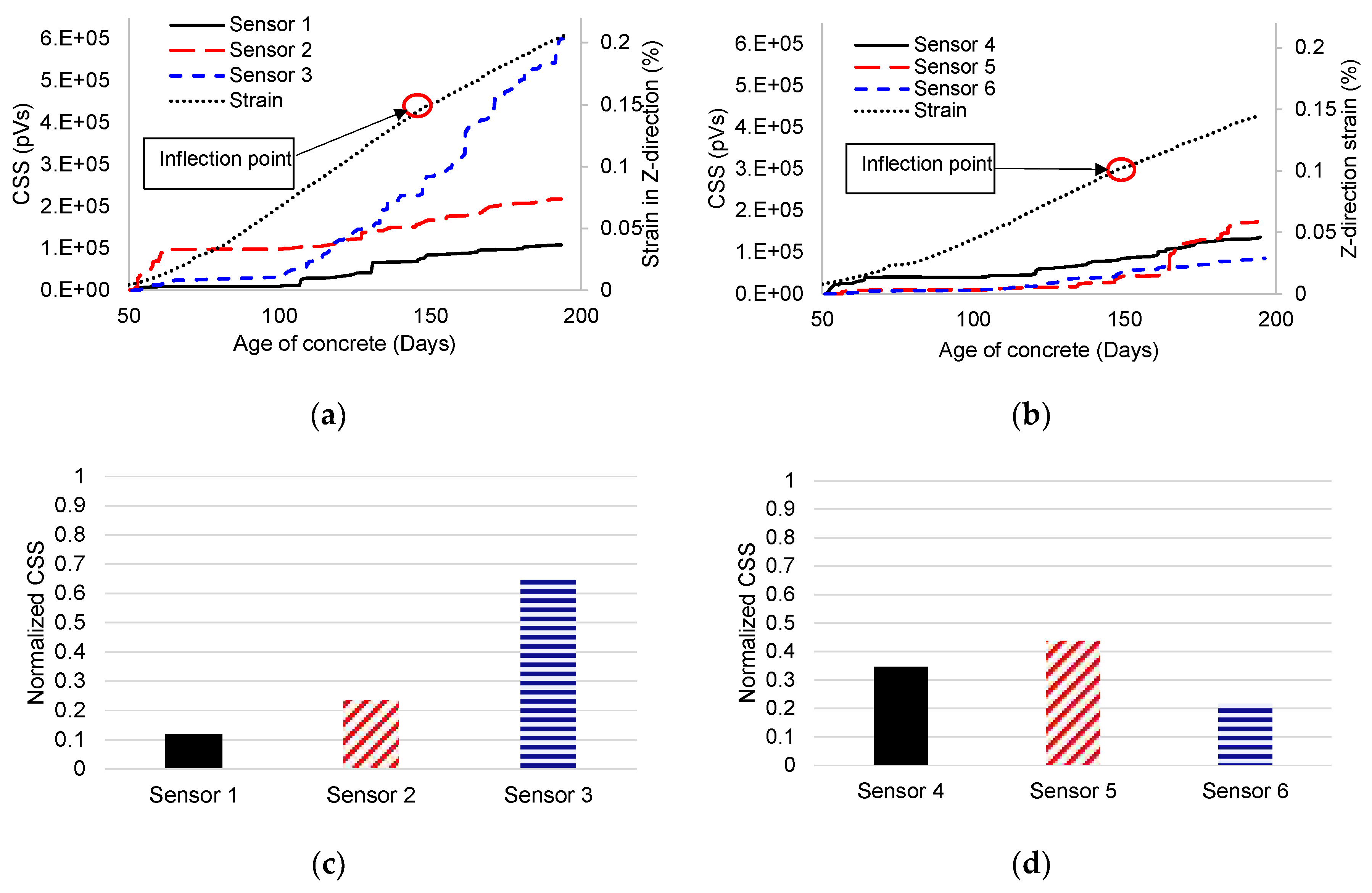
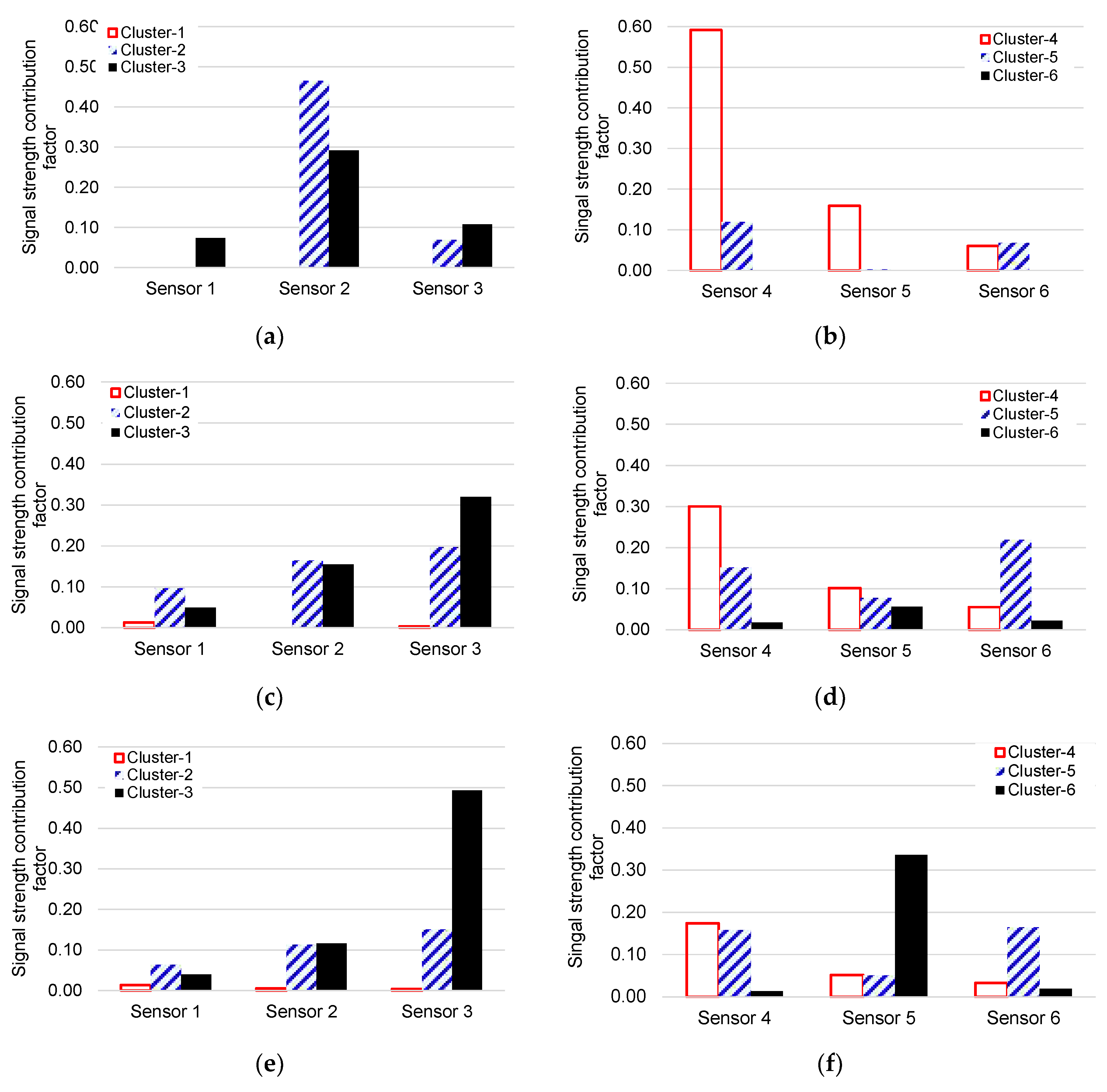
• A significant portion of the AE data (in terms of cumulative signal strength) in the confined specimen was recorded by sensor 3, which was located at mid-thickness. However, the portion of cumulative signal strength for the corresponding sensor at mid-thickness of the unconfined specimen was less in comparison to the other two sensors in that specimen. This agrees with expectations, as the confined specimen exhibited increased out-of-plane expansion in comparison to the unconfined specimen, meaning that the crack distribution is expected to be more concentrated near mid-thickness of the confined specimen than near the reinforcement layers.
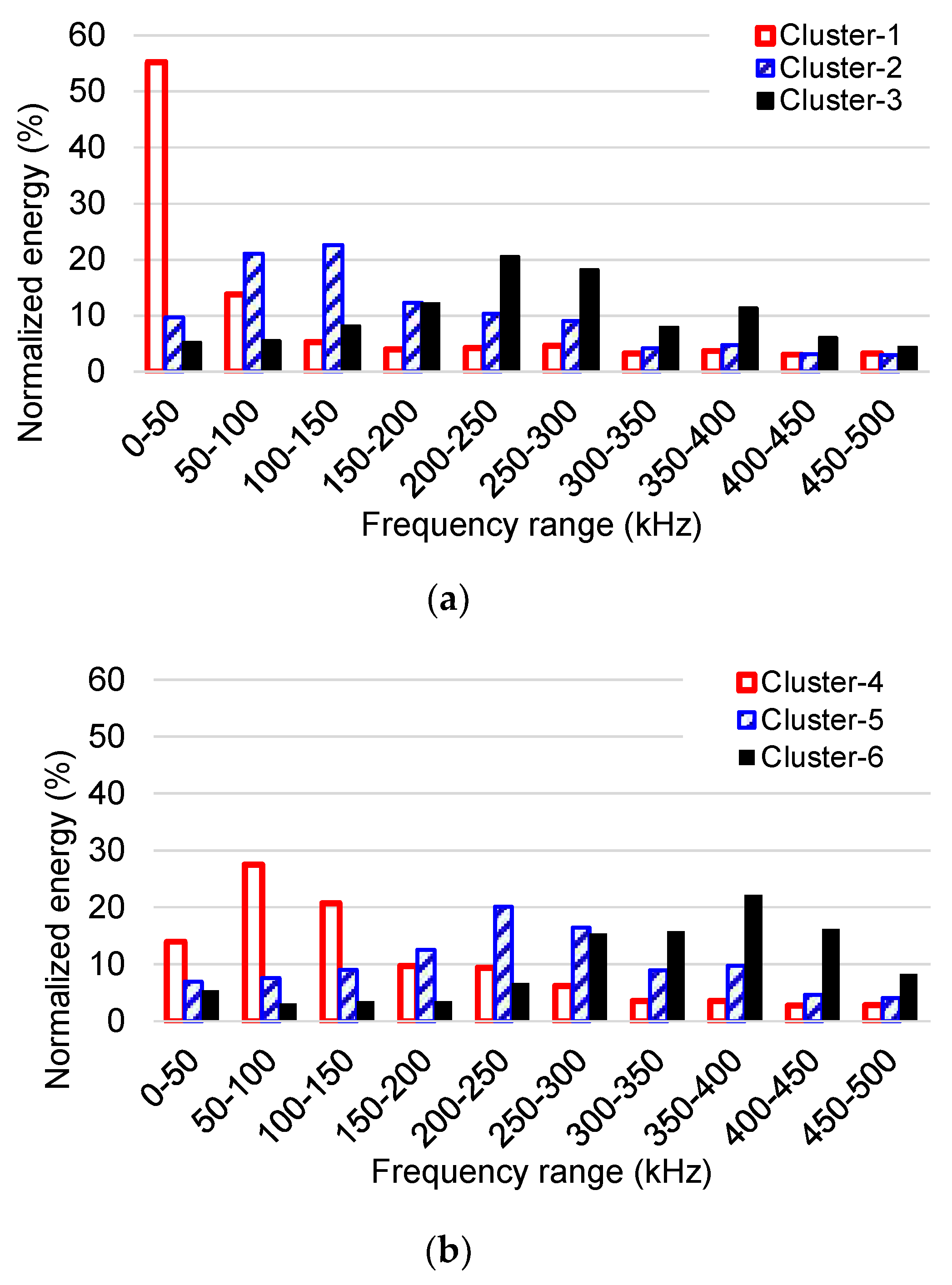
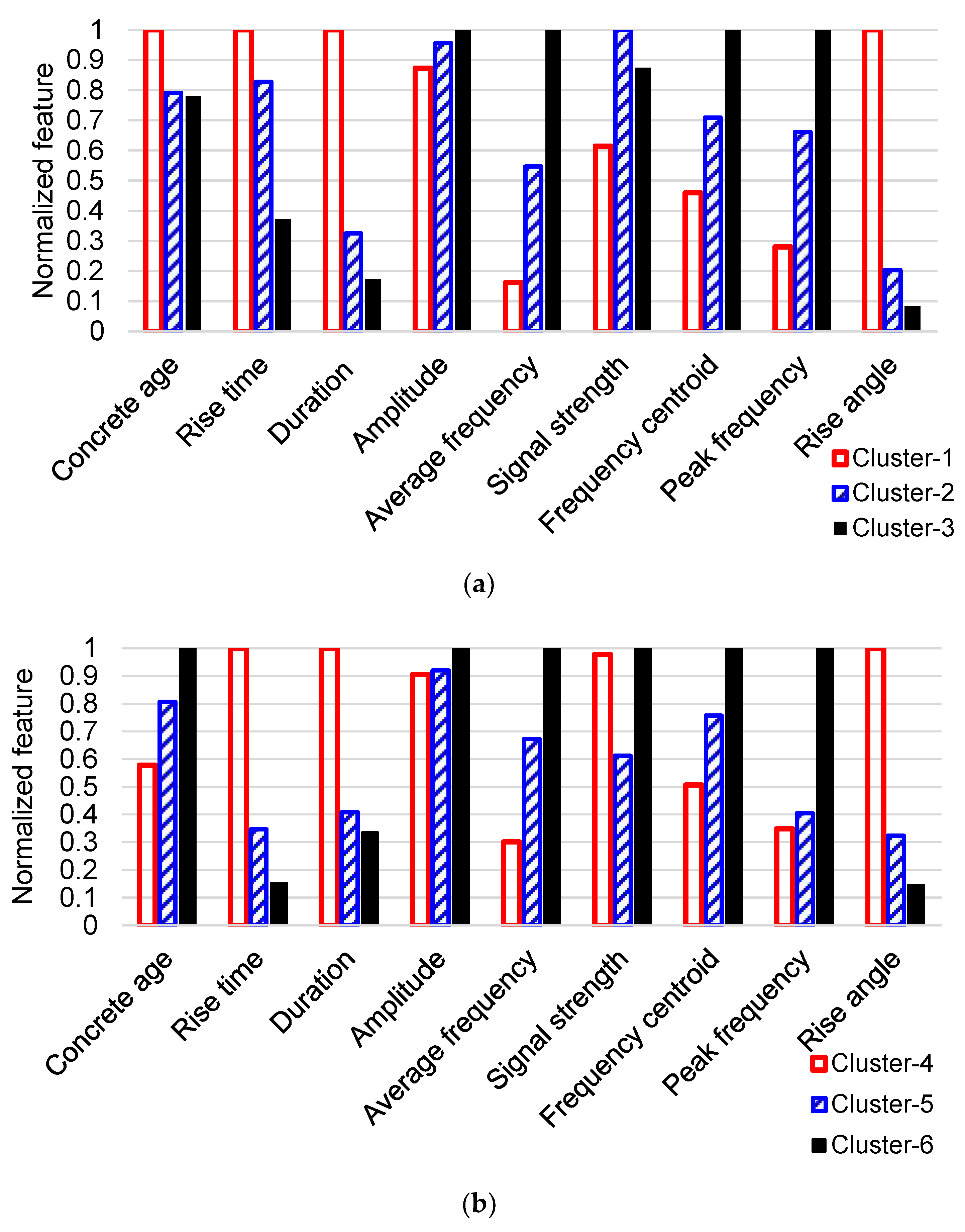
• The frequency contents of signals in the confined and unconfined specimens evolved from low to high frequency with the age of concrete although this evolution started later in the confined specimen than the unconfined specimen. Since the high-frequency AE signals have been associated to the cracking in aggregates [17], different crack mechanisms in aggregate for the confined and unconfined specimens are expectable. However, there are different contradictory ASR cracking hypotheses that have been proposed by the researchers [33,34,35,36,37,38,41,42,43].
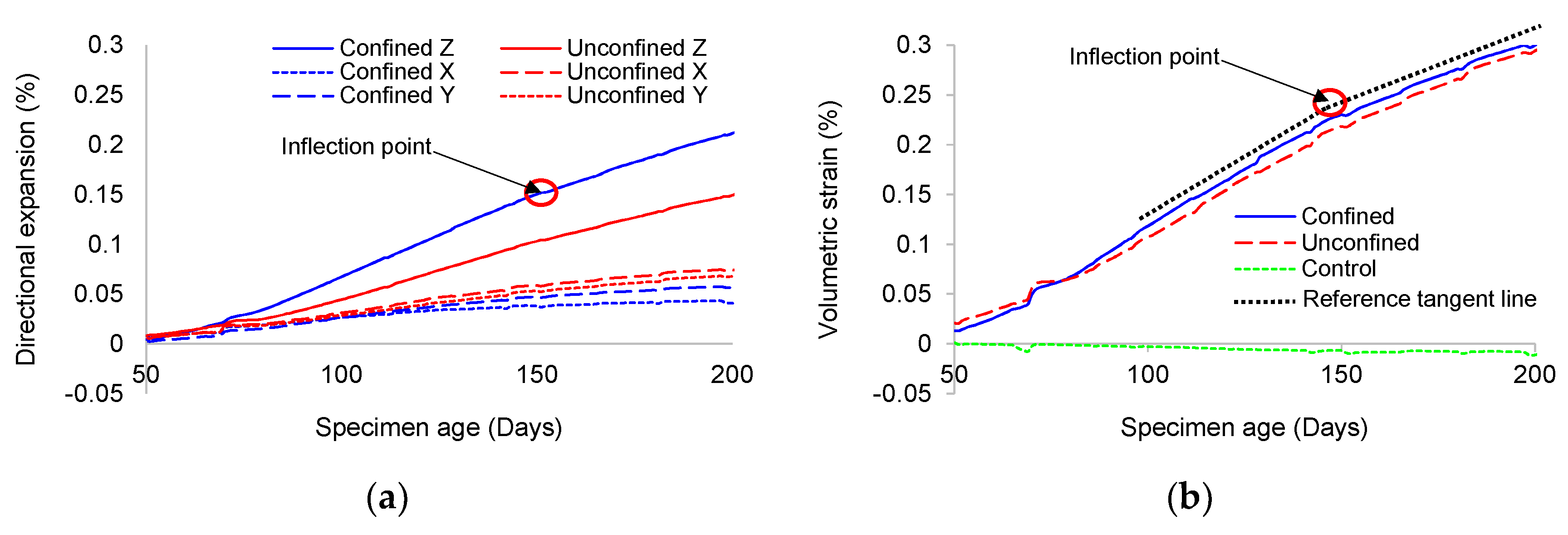
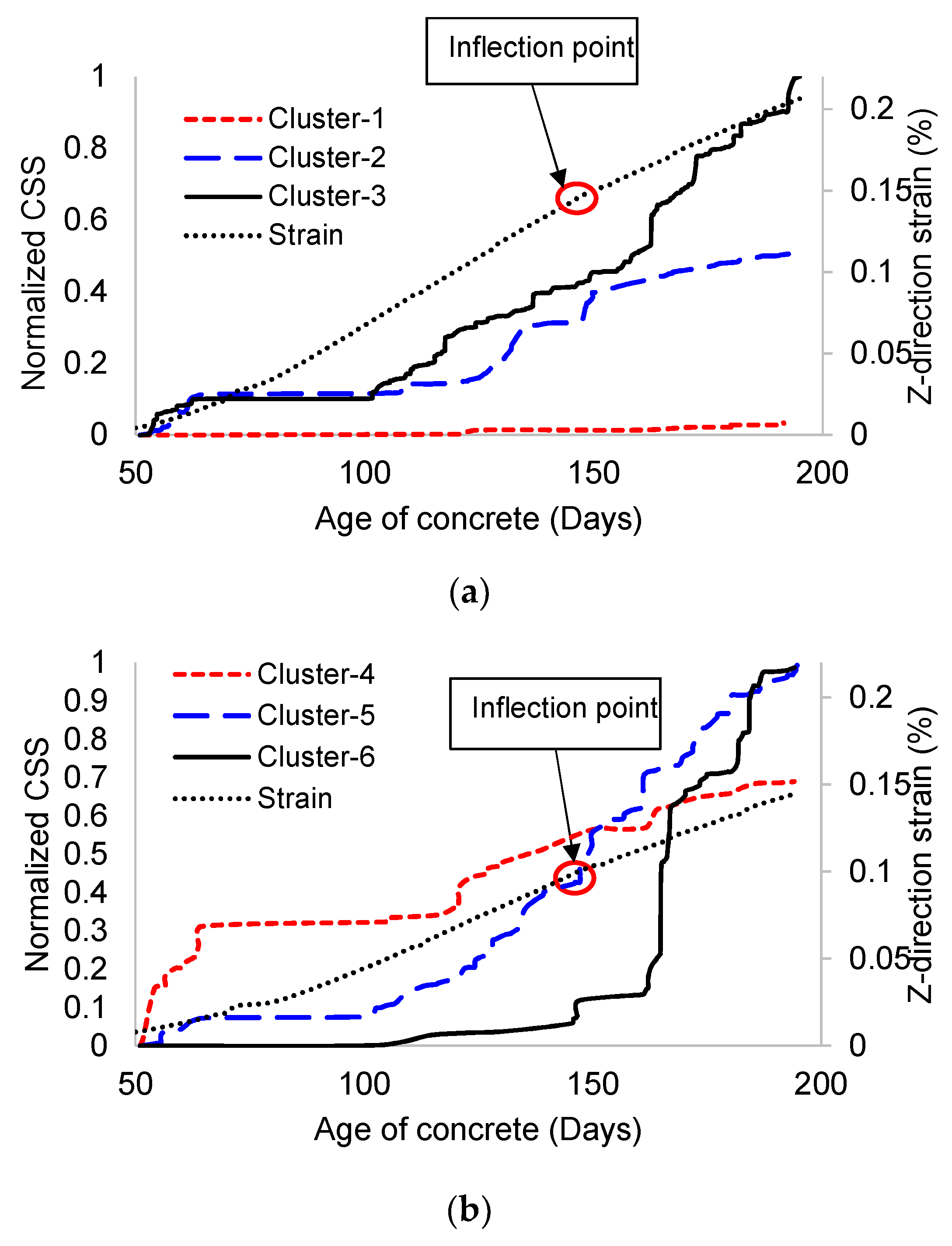
• There is a coincident point observed in the strain curves and the CSS of Cluster-3 in the confined specimen and Cluster-6 in the unconfined specimen. The CSS rate in terms of concrete age increases at the time (around 150 days), when the strain rate is decreasing. This point is named as inflection point of strain curve, where the curvature of strain curve changes from positive to negative. The inflection point location in terms of concrete age depends on the kinetic of ASR reaction and diffusion process. Determining the inflection point, latency and characteristic time are experimentally estimated, which are the two important modeling parameters. According to the results of AE data and clustering, the inflection point location in terms of concrete age could be estimated from the variation in CSS rate change of clustered AE data.
• Monitoring of a structural system with acoustic emission can provide useful information regarding condition based maintenance and/or retrofit. For example, one potential time of action for treating affected structures is around the inflection point in the volumetric strain curve which can be approximated through acoustic emission data. This point coincided with observation of first visible surface cracking. After identifying the time of action, treatment methods may be implemented to mitigate the effects of ASR. Injection of lithium solution is a chemical alternative to mitigate ASR provided that enough solution penetration in the structure can be achieved. Another method is to remove moisture through coatings and sealers such as silane sealers and bituminous or elastomeric coatings. After conducting these methods, structures should be monitored for enough time to evaluate the efficiency of the method or methods.

References

1. Schmidt, J.W.; Hansen, S.G.; Barbosa, R.A.; Henriksen, A. Novel shear capacity testing of ASR damaged full scale concrete bridge. Eng. Struct. 2014, 79, 365–374. [Google Scholar] [CrossRef]
2. Clark, L. Critical Review of the Structural Implications of the Alkali Silica Reaction in Concrete; Contactor Report 169; Transportation and Road Research Laboratory, Department of Transport: Crowthone, UK, 1989. [Google Scholar]
3. Bach, F.; Thorsen, T.S.; Nielsen, M. Load-carrying capacity of structural members subjected to alkali-silica reactions. Constr. Build. Mater. 1993, 7, 109–115. [Google Scholar] [CrossRef]
4. Bakker, J. Control of ASR related risks in the Netherlands. In Proceedings of the 13th International Conference on Alkali-Aggregate Reaction in Concrete, Trondheim, Norway, 16–20 June 2008; pp. 21–31. [Google Scholar]
5. Charlwood, R.; Solymar, S.; Curtis, D. A review of alkali aggregate reactions in hydroelectric plants and DAMS. In Proceedings of the International Conference of Alkali-Aggregate Reactions in Hydroelectric Plants and Dams, Fredericton, NB, Canada, 28 September–2 October 1992; Volume 129. [Google Scholar]
6. Saouma, V.E.; Hariri-Ardebili, M.A. A proposed aging management program for alkali silica reactions in a nuclear power plant. Nucl. Eng. Des. 2014, 277, 248–264. [Google Scholar] [CrossRef]
7. Takakura, T.; Ishikawa, T.; Mitsuki, S.; Matsumoto, N.; Takiguchi, K.; Masuda, Y.; Nishiguchi, I. Investigation on the expansion value of turbine generator foundation affected by alkali-silica reaction. In Proceedings of the 18th International Conference on Structural Mechanics in Reactor Technology (SMiRT), Beijing, China, 7–12 August 2005; pp. 2061–2068. [Google Scholar]
8. Takakura, T.; Masuda, H.; Murazumi, Y.; Takiguchi, K.; Masuda, Y.; Nishiguchi, I. Structural soundness for turbine-generator foundation affected by alkali-silica reaction and its maintenance plans. In Proceedings of the 19th International Conference on Structural Mechanics in Reactor Technology (SMiRT), Toronto, ON, Canada, 12–17 August 2007. [Google Scholar]
9. Tcherner, J.; Aziz, T. Effects of AAR on seismic assessment of nuclear power plants for life extensions. In Proceedings of the 20th International Conference on Structural Mechanics in Reactor Technology (SMiRT), Espoo, Finland, 9–14 August 2009; pp. 1–8. [Google Scholar]
10. Charlwood, R. Predicting the long term behaviour and service life of concrete dams, Long Term Behaviour of Dams. In Proceedings of the 2nd International Conference, Graz, Austria, 12–13 October 2009. [Google Scholar]
11. Abdelrahman, M.; ElBatanouny, M.K.; Ziehl, P.; Fasl, J.; Larosche, C.J.; Fraczek, J. Classification of alkali–silica reaction damage using acoustic emission: A proof-of-concept study. Constr. Build. Mater. 2015, 95, 406–413. [Google Scholar] [CrossRef]
12. Garcia-Diaz, E.; Riche, J.; Bulteel, D.; Vernet, C. Mechanism of damage for the alkali–silica reaction. Cem. Concr. Res. 2006, 36, 395–400. [Google Scholar] [CrossRef]
13. Sargolzahi, M.; Kodjo, S.A.; Rivard, P.; Rhazi, J. Effectiveness of nondestructive testing for the evaluation of alkali–silica reaction in concrete. Constr. Build. Mater. 2010, 24, 1398–1403. [Google Scholar] [CrossRef]
14. Anay, R.; Soltangharaei, V.; Assi, L.; DeVol, T.; Ziehl, P. Identification of damage mechanisms in cement paste based on acoustic emission. Constr. Build. Mater. 2018, 164, 286–296. [Google Scholar] [CrossRef]
15. Soltangharaei, V.; Anay, R.; Assi, L.; Ziehl, P.; Matta, F. Damage identification in cement paste amended with carbon nanotubes. AIP Conf. Proc. 2018, 1949, 030006. [Google Scholar] [CrossRef]
16. Lokajíček, T.; Přikryl, R.; Šachlová, Š.; Kuchařová, A. Acoustic emission monitoring of crack formation during alkali silica reactivity accelerated mortar bar test. Eng. Geol. 2017, 220, 175–182. [Google Scholar] [CrossRef]
17. Farnam, Y.; Geiker, M.R.; Bentz, D.; Weiss, J. Acoustic emission waveform characterization of crack origin and mode in fractured and ASR damaged concrete. Cem. Concr. Compos. 2015, 60, 135–145. [Google Scholar] [CrossRef]
18. Rajabipour, F.; Giannini, E.; Dunant, C.; Ideker, J.H.; Thomas, M.D. Alkali–silica reaction: Current understanding of the reaction mechanisms and the knowledge gaps. Cem. Concr. Res. 2015, 76, 130–146. [Google Scholar] [CrossRef]
19. Weise, F.; Katja, V.; Pirskawetz, S.; Dietmar, M. Innovative measurement techniques for characterising internal damage processes in concrete due to ASR. In Proceedings of the International Conference on Alkali Aggregate Reaction (ICAAR), University of Texas, Austin, TX, USA, 20–25 May 2012. [Google Scholar]
20. Morenon, P.; Multon, S.; Sellier, A.; Grimal, E.; Hamon, F.; Bourdarot, E. Impact of stresses and restraints on ASR expansion. Constr. Build. Mater. 2017, 140, 58–74. [Google Scholar] [CrossRef]
21. Saouma, V.E.; Hariri-Ardebili, M.A.; Le Pape, Y.; Balaji, R. Effect of alkali–silica reaction on the shear strength of reinforced concrete structural members. A numerical and statistical study. Nucl. Eng. Des. 2016, 310, 295–310. [Google Scholar] [CrossRef]
22. Hayes, N.W.; Gui, Q.; Abd-Elssamd, A.; Le Pape, Y.; Giorla, A.B.; Le Pape, S.; Giannini, E.R.; Ma, Z.J. Monitoring Alkali-Silica Reaction Significance in Nuclear Concrete Structural Members. J. Adv. Concr. Technol. 2018, 16, 179–190. [Google Scholar] [CrossRef]
23. Hsu, N. Characterization and calibration of acoustic emission sensors. Mater. Eval. 1981, 39, 60–68. [Google Scholar]
24. Express-8 AE System User Manual; Mistras Group, Inc.: Princeton Junction, NJ, USA, 2014.
25. Murtagh, F.; Legendre, P. Ward’s hierarchical agglomerative clustering method: Which algorithms implement Ward’s criterion? J. Classif. 2014, 31, 274–295. [Google Scholar] [CrossRef]
26. Tan, P.N.; Steinbach, M.; Karpatne, A.; Kumar, V. Introduction to Data Mining, 2nd ed.; Pearson Education: New York, NY, USA, 2018; ISBN 978-013-312-890-1. [Google Scholar]
27. Saouma, V.; Perotti, L. Constitutive model for alkali-aggregate reactions. ACI Mater. J. 2006, 103, 194. [Google Scholar]
28. Ulm, F.J.; Coussy, O.; Kefei, L.; Larive, C. Thermo-chemo-mechanics of ASR expansion in concrete structures. J. Eng. Mech. 2000, 126, 233–242. [Google Scholar] [CrossRef]
29. Fowler, T.J.; Blessing, J.A.; Conlisk, P.J.; Swanson, T.L. The MONPAC system. J. Acoust. Emiss. 1989, 8, 1–8. [Google Scholar]
30. ElBatanouny, M.K.; Ziehl, P.H.; Larosche, A.; Mangual, J.; Matta, F.; Nanni, A. Acoustic emission monitoring for assessment of prestressed concrete beams. Constr. Build. Mater. 2014, 58, 46–53. [Google Scholar] [CrossRef]
31. Aggelis, D.; Soulioti, D.; Gatselou, E.; Barkoula, N.-M.; Matikas, T.E. Monitoring of the mechanical behavior of concrete with chemically treated steel fibers by acoustic emission. Constr. Build. Mater. 2013, 48, 1255–1260. [Google Scholar] [CrossRef]
32. Xargay, H.; Folino, P.; Nuñez, N.; Gómez, M.; Caggiano, A.; Martinelli, E. Acoustic Emission behavior of thermally damaged Self-Compacting High Strength Fiber Reinforced Concrete. Constr. Build. Mater. 2018, 187, 519–530. [Google Scholar] [CrossRef]
33. Pan, J.; Feng, Y.; Wang, J.; Sun, Q.; Zhang, C.; Owen, D.J. Modeling of alkali-silica reaction in concrete: A review. Front. Struct. Civ. Eng. 2012, 6, 1–18. [Google Scholar] [CrossRef]
34. Hanson, W. Studies Relating To the Mechanism by Which the Alkali-Aggregate Reaction Produces Expansion in Concrete. J. Am. Concr. Inst. 1944, 40, 213–228. [Google Scholar]
35. McGowan, J.K. Studies in Cement-Aggregate Reaction XX, the Correlation between Crack Development and Expansion of Mortar. Aust. J. Appl. Sci. 1952, 3, 228–232. [Google Scholar]
36. Bazant, Z.P.; Steffens, A. Mathematical model for kinetics of alkali–silica reaction in concrete. Cem. Concr. Res. 2000, 30, 419–428. [Google Scholar] [CrossRef] [Green Version]
37. Dron, R.; Brivot, F. Thermodynamic and kinetic approach to the alkali-silica reaction. Part 1: Concepts. Cem. Concr. Res. 1992, 22, 941–948. [Google Scholar] [CrossRef]
38. Idorn, G.M. A discussion of the paper “Mathematical model for kinetics of alkali-silica reaction in concrete” by Zdenek P. Bazant and Alexander Steffens. Cem. Concr. Res. 2001, 7, 1109–1110. [Google Scholar] [CrossRef]
39. Jun, S.S.; Jin, C.S. ASR products on the content of reactive aggregate. J. Civ. Eng. 2010, 14, 539–545. [Google Scholar] [CrossRef]
40. Goltermann, P. Mechanical predictions of concrete deterioration; Part 2: Classification of crack patterns. Mater. J. 1995, 92, 58–63. [Google Scholar]
41. Ichikawa, T.; Miura, M. Modified model of alkali-silica reaction. Cem. Concr. Res. 2007, 37, 1291–1297. [Google Scholar] [CrossRef]
42. Ponce, J.M.; Batic, O.R. Different manifestations of the alkali-silica reaction in concrete according to the reaction kinetics of the reactive aggregate. Cem. Concr. Res. 2006, 36, 1148–1156. [Google Scholar] [CrossRef]
43. Escalante-Garcıa, J.; Sharp, J. The microstructure and mechanical properties of blended cements hydrated at various temperatures. Cem. Concr. Res. 2001, 31, 695–702. [Google Scholar] [CrossRef]
Figure 1. Test specimens.
Applsci 08 02148 g001
Figure 2. Acoustic emission (AE) sensor locations. (a) Internal AE sensors (broadband); (b) External AE sensors (resonant); (c) Internal sensors 3 and 6 installation; (d) Internal sensors 1, 2, 4 and 5 installation.
Applsci 08 02148 g002
Figure 3. Clustering procedure. (a) Energy-frequency based feature extraction; (b) Flow chart of data clustering steps.
Applsci 08 02148 g003
Figure 4. Strain distribution of specimens versus concrete age. (a) Directional expansion; (b) Volumetric strain.
Applsci 08 02148 g004
Figure 5. Amplitude and cumulative signal strength of AE data in terms of concrete age. (a) Confined specimen; (b) Unconfined specimen; (c) Control specimen.
Applsci 08 02148 g005
Figure 6. Cumulative signal strength (CSS) contribution for sensors. (a) CSS vs. age of concrete for confined specimen; (b) CSS vs. age of concrete for unconfined specimen; (c) Normalized CSS for confined specimen; (d) Normalized CSS for unconfined specimen.
Applsci 08 02148 g006
Figure 7. Clustering dendrograms. (a) Confined specimen; (b) Unconfined specimen.
Applsci 08 02148 g007
Figure 8. Clusters in principle component dimensions. (a) Confined specimen; (b) Unconfined specimen.
Applsci 08 02148 g008
Figure 9. Average normalized signal energy in frequency domain. (a) Confined specimen; (b) Unconfined specimen.
Applsci 08 02148 g009
Figure 10. Normalized signal features. (a) Confined specimen; (b) Unconfined specimen.
Applsci 08 02148 g010
Figure 11. Normalized cumulative signal strength. (a) Confined specimen; (b) Unconfined specimen.
Applsci 08 02148 g011
Figure 12. Distribution of total AE signal strength in terms of clusters and sensors. (a) Confined specimen at age of 66 days; (b) Unconfined specimen at age of 66 days; (c) Confined specimen at age of 150 days; (d) Unconfined specimen at age of 150 days; (e) Confined specimen at age of 195 days; (f) Unconfined specimen at age of 195 days.
Applsci 08 02148 g012