Design Considerations for Murine Retinal Imaging Using Scattering Angle Resolved Optical Coherence Tomography

Featured Application

Scattering angle resolved optical coherence tomography offers a new contrast mechanism for murine retinal imaging.

Abstract

Optical coherence tomography (OCT), an optical imaging approach enabling cross-sectional analysis of turbid samples, is routinely used for retinal imaging in human and animal models of diseases affecting the retina. Scattering angle resolved (SAR-)OCT has previously been demonstrated as offering additional contrast in human studies, but no SAR-OCT system has been reported in detail for imaging the retinas of mice. An optical model of a mouse eye was designed and extended for validity at wavelengths of light around 1310 nm; this model was then utilized to develop a SAR-OCT design for murine retinal imaging. A Monte Carlo technique simulates light scattering from the retina, and the simulation results are confirmed with SAR-OCT images. Various images from the SAR-OCT system are presented and utility of the system is described. SAR-OCT is demonstrated as a viable and robust imaging platform to extend utility of retinal OCT imaging by incorporating scattering data into investigative ophthalmologic analysis.

1. Introduction

Optical coherence tomography (OCT) is an optical imaging technique that utilizes the coherence properties of light to obtain cross-sectional images of turbid samples by interfering sample and reference arms [1]. OCT has been used in disciplines ranging from additive manufacturing to cardiology.

OCT has become the standard of care in ophthalmology and is routinely used to monitor changes in the retina and optic nerve [2]. However, standard clinical OCT systems are generally unable to detect changes in backscattered light’s scattering angle.

Angle-resolved approaches measure angular distribution of backscattered light, which changes based on tissue anisotropy. A rich literature exists concerning angle-resolved imaging of apoptotic and necrotic tissues specifically, and these studies demonstrate the potential clinical relevance of a scattering-angle resolved imaging platform. One study examined forward scattering changes (5–90 degrees) due to mitochondrial swelling due to oxidative stress in suspensions of intact murine mammary carcinoma cells and found that treated cells scattered less light at low angles [3]. Similarly, another study reports an increase in the ratio of high- to low-angle light scattering (forward forward) for induced mitochondrial fission [4]. However, two other studies reported by the same authors indicate a decrease in the same ratio in apoptotic cells [5,6]. In each case, shifts in scattering angle are associated specifically with changes in mitochondrial morphology, underscoring importance of mitochondria in light scattering [7].

Previously, angle-resolved interferometric imaging approaches have been used to detect sub-wavelength cellular properties such as the size distribution of nuclei and more recently to characterize nuclear morphology, in situ, of both a rodent model for esophageal carcinogenesis and murine retinas [8,9]. Thus, while several cell culture and ex-vivo tissue studies have been reported involving angle-resolved imaging, similar optical imaging techniques have not been extensively explored for retinal imaging.

Other publication threads also suggest a pathway to identify retinal scattering changes. First, a non-human primate study introduced a new contrast measure (“reflectance index”) that decreases in eyes in response to elevated intraocular pressure [10]. In a follow-up study, a refined measure of reflection ratios (“normalized reflectance index”) was introduced and reveals an early correlation with pre-perimetric glaucoma in human subjects [11]. Investigators suggested that a candidate biological mechanism for observed changes is modification of the scattering properties of sub-resolution cellular components. Consequently, a third study was conducted in which a scattering angle resolved (SAR-)OCT system was designed and constructed to inspect the optical properties of healthy human retinas [12]. In this study, ocular regions with lower retinal ganglion cell density correlate with the SAR-index, indicating sensitivity of SAR-OCT to morphological variations. SAR-OCT has been demonstrated to detect sub-resolution light scattering variations in the retina. More recent work in angle-resolved OCT imaging finds that multi-directional pathlength-multiplexed OCT imaging may be used to assess the directional reflectivity of retinal layers in human subjects [13], and for obtaining directional blood flow information [14]. An opportunity is recognized for exploring utility SAR-OCT as a new contrast mechanism in healthy and diseased retinas, with potential applications to detect a variety of neurodegenerative diseases that affect retinal morphology.

Developing such a system for mouse retina imaging is a natural step in development of SAR-OCT frameworks. The SAR-OCT system previously reported is for human retinal imaging, but due to animal availability and ease of access for proof-of-concept work in accelerated studies, an animal SAR-OCT system for ocular imaging is a valuable tool to examine how diseases affect the scattering properties of the retina. Several well-documented murine disease models—both induced and transgenic—have retinal pathologies.

In fact, many OCT studies involve murine disease models because of the mouse eye is strikingly similarity to the human eye (in particular, over that of a rat). The mouse eye has a large numerical aperture and thus higher order aberrations that resemble that in humans [15]. Although optical properties of the murine eye have been explored at short wavelengths [16,17], the mouse eye has not been characterized at wavelengths in the near infrared (NIR) wavelength range.

This paper describes a basic optical model for the murine eye in the NIR range and then uses that model to develop an SAR-OCT system for mouse retinal imaging.

2. Materials and Methods

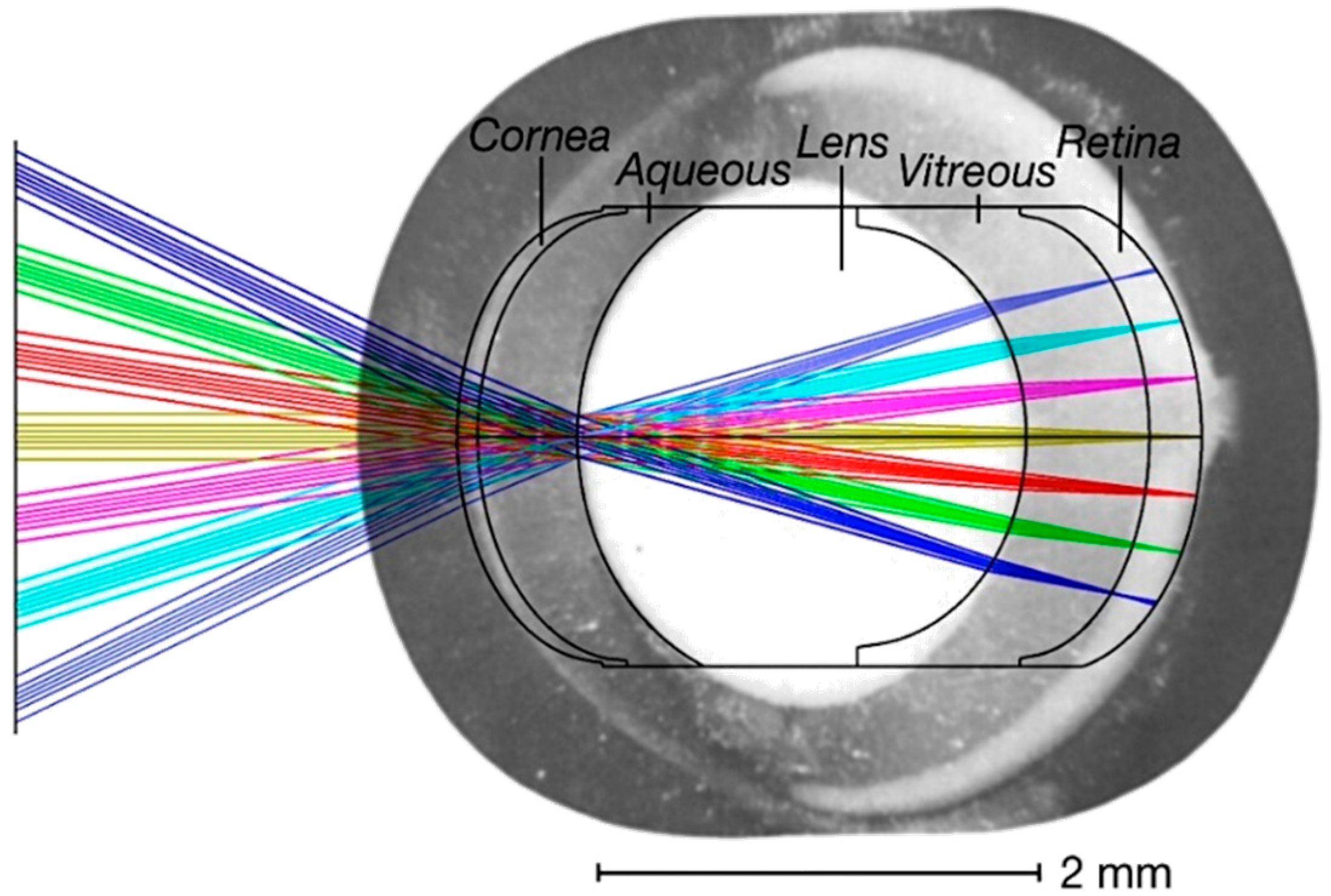
2.1. Murine Eye Model

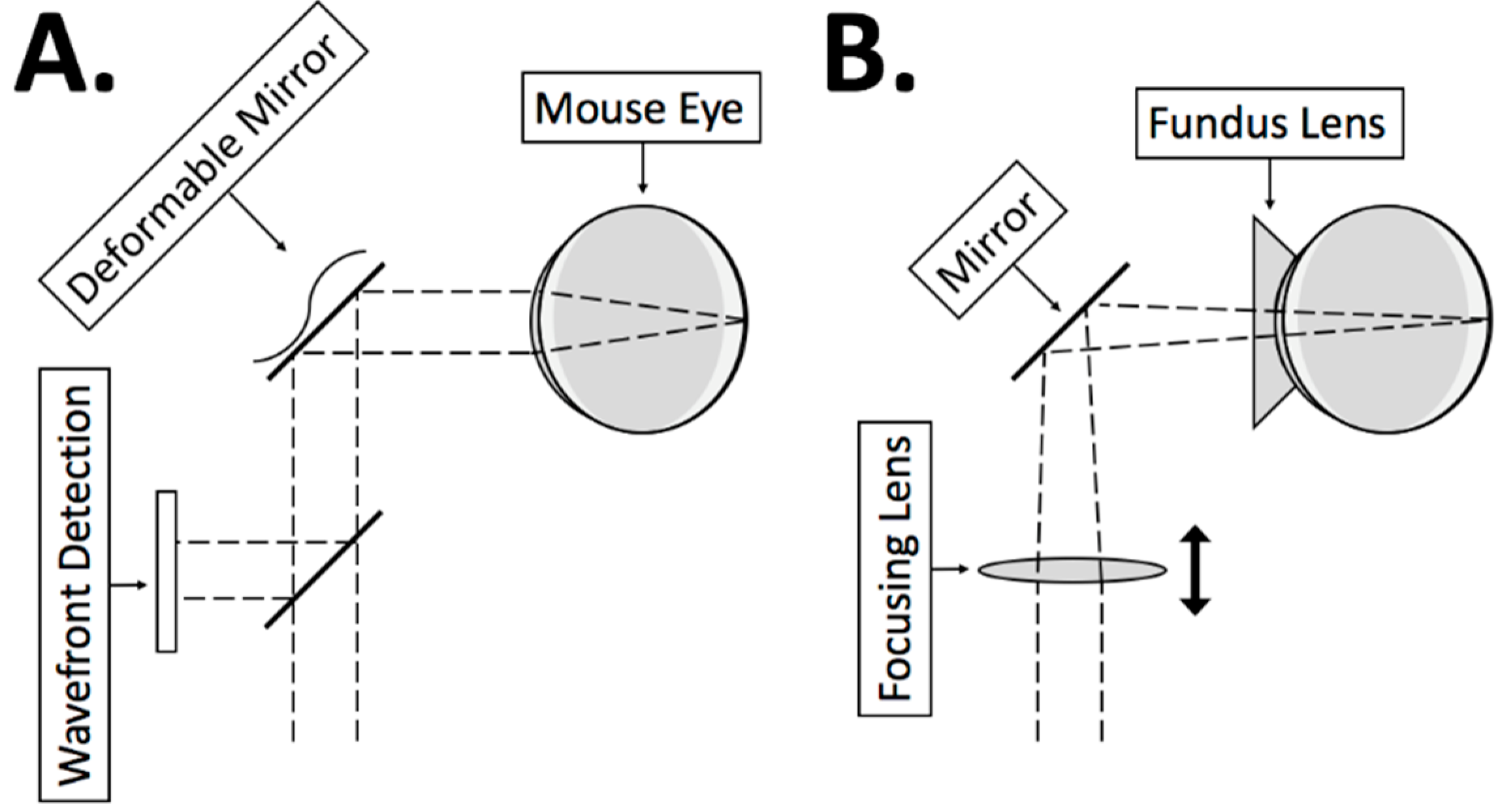
To develop a murine eye model, the ocular components’ radii of curvature were constructed in OpticStudio (Zemax) as reported by Remtulla [16] and refractive indices of the ocular components were modeled. Remtullah also reported the refractive index of each layer of the murine eye at four wavelengths. These data were extrapolated to the NIR by fitting the four data points from Remtullah to Conrady’s dispersion equation [18]:

$$n\left(\lambda \right)=n_0+\frac{B}{\lambda }+\frac{C}{{\lambda }^{3.5}}.$$

(1)

In Conrady’s Equation (1), n is the refractive index, n₀ is the refractive index as λ approaches ∞, B (μm) is a parameter affecting the curvature and amplitude of the refractive index at visible wavelengths, and C (μm^3.5) influences refractive index in the UV. The Conrady dispersion formula is well suitedfor transparent materials such as the murine eye. The fit yielded the parameters and refractive indices listed in the corresponding section in Table 2 in Section 3.1.

2.2. System Design

The materials and methods for designing and constructing a SAR-OCT mouse retinal imager (Figure 1) are described.

Similar to the Wang design, the SAR-OCT design described here is a fiber-based system for ease of transport to the operating room. Because bulk optics systems are difficult and time-consuming to align single mode fiber optics were utilized when possible. SMF-28e fibers are used here which transmit the 1310 nm (±70 nm) broadband swept source (100 kHz repetition rate, 25 mW output, Axsun) in a single mode. The Axsun laser bandwidth is greater and the sweep repetition rate is faster than that of the Wang design. FC-APC fiber connections are employed to minimize any reflected light from fiber–fiber interfaces and reduce ghost interference signals.

A 90:10 fiber coupler directs 90% of the laser’s output to the sample arm optics and 10% to the reference arm (Figure 1) to give 15 mW average power incident on the mouse cornea. Each arm of the interferometer has a fiber circulator with three arms. Light entering arm 1 exits arm 2, and light returning to arm 2 exits arm 3. After sample and reference optics, the light is interfered in a 50:50 fiber coupler, and each output is measured by a balanced detection scheme. Balanced detection eliminates the background signal to isolate the interference fringe.

Concerning the laser source, a swept source OCT system typically has some advantages over spectral domain for SAR-OCT. The relevant optical design parameter for the pathlength multiplexing element (PME; described in Section 2.2.5) and SAR-OCT is the scan range. In swept source OCT, scan range is given by instantaneous coherence length of the swept laser source. In comparison, for spectral domain OCT, scan range is given by spectral resolving power of the readout spectrometer. In many OCT spectrometers, the scan range is on the order of 4–5 mm. Since the scan range of many swept laser sources is on the order of 10–100 mm, PME design and corresponding pathlength difference between distinct angular paths is greater than that in spectral domain OCT. Thus, most swept-source OCT systems provide greater PME design flexibility and separation of angular paths compared to spectral domain approaches.

2.2.1. 2D MEMS Mirror

Most murine retinal images reported in the scientific literature include post-objective scanning systems. In these systems, galvanometers are placed between the final lens (objective) and the retina. Collimated light is directed by mirrors at different angles to reach different parts of the retina. This design limits the field of view of the OCT systems because the ocular pupil clips OCT source light at the system’s most extreme angle.

This problem can be mitigated by placing the mirrors at conjugates to the ocular pupil plane and thus steering the beam beyond the aperture of the pupil. However, engineers using this approach have typically used two-mirror galvanometer systems. In this case, the designer must choose either the slow axis, the fast axis, or somewhere in-between as a conjugate plane to the ocular pupil. The slow-axis has historically been chosen to maximize collection efficiency and minimize vignetting [20]. New approaches to limit vignetting and maximize collection efficiency have included pupil tracking to control where the beam enters the pupil [21].

Dual-axis MEMS mirrors have been used in OCT catheter designs and free-space optical setups [22,23], but adoption of dual axis-mirrors for retinal imaging has been more slow. Recent examples include hand-held OCT retina and anterior segment imaging systems [24,25]. The system reported here is the first OCT system to use dual-axis MEMS mirror scanning for mouse retinal imaging, and first reported in less detail in 2017 [19].

2.2.2. Corneal Contact

Many OCT systems, including almost all human retinal imaging systems, are non-contact systems meaning the objective lens does not make contact with the subject’s cornea. This is particularly helpful for human subjects who may be told to hold still for several seconds while an OCT image is captured. Patient discomfort is thus minimized by removing the need for an index matching medium between the objective and the patient’s cornea. Mice are typically anesthetized when their retinas are imaged using OCT, thus allowing for a corneal contact system.

One issue with non-contact OCT retinal imagers is that the beam wavefront is subject to the natural aberrations of the eye—the air–cornea and aqueous–lens interfaces providing most of the optical power. The mouse eye introduces significant amounts of spherical aberration and coma, with astigmatism [26]. In conflicting reports, the murine eye has been reported as both myopic and hyperopic [15,26]. Significant longitudinal chromatic aberrations exist and the mouse eye has a numerical aperture of 0.5, as opposed to a human eye’s 0.2 [15].

A murine retinal imager must account for these aberrations to obtain quality images. Generally, there are two approaches to limiting the effect of aberrations in murine retinal imaging.

First, wavefront sensing and adaptive optics can improve the spot size of the beam on the retina and account for aberrations in the eye. Such systems have been reported for human retinal OCT and scanning laser ophthalmoscope systems [27,28] and for murine retinal OCT systems [29,30]. Classically, these OCT systems employ a wavefront sensor (either with a Shack–Hartmann wavefront sensor or computationally). Based on the sensed wavefront characteristics, an adaptive optic element (e.g., deformable mirror, spatial light modulator) will adaptively alter the incident beam wavefront until the reflected beam has a high-quality wavefront. This intervention ensures that the beam spot size on the retina is small and thus improves spatial resolution. Although these systems are powerful tools, they are more costly and may be slow to make their way to a clinical setting.

The second approach is to design a corneal contact system to limit the effect of aberrations from the air-cornea interface [31]. This interface has the most optical power and contributes significantly to optical aberrations in the mouse eye [16]. For a more cost-effective approach to limiting aberrations, a corneal contact lens can be index matched to the cornea [32].

For non-contact systems, the incident beam is collimated (or its wavefront adjusted with adaptive optics) and relies on the natural optics of the eye to focus on the retina. By removing the optical power of the cornea with a contact lens, light should have some positive (convergent) power upon entering the eye to focus on the retina. Figure 2 presents non-contact and contact designs.

A custom contact lens was fabricated (Optics Technology, Inc.) by etching down a BK7 window with an anti-reflective (AR) coating. The AR coating was maintained on the non-contact side, and a concave surface was formed at the opposite side (radius = 2 mm). The AR coating limits any unwanted reflections from being coupled back into the fiber interferometer. The concave surface is index-matched to the cornea using methyl cellulose.

2.2.3. Focusing Lens

Because the system uses a contact lens, light should have some optical power upon entering the eye. However, given the variability of optical properties across different mice, particularly the thickness of ocular components, it would be advantageous to have a movable lens to optimize spot size on the retina. Thus, the lens providing the power is placed on a translation stage. For longer eyes, the lens is translated toward the mouse to move the focal plane deeper into the eye, and vice versa. This lens and translation mount are placed before the 2D MEMS mirror, thus the diameter of the beam on the mirror (and the ocular pupil plane conjugate to the pupil) varies with the translation of the lens. Although the beam size on the mirror varies, it never is clipped by the mirror.

2.2.4. Dispersion Compensation

Group delay dispersion mismatch between the sample and reference arms can negatively affect OCT images by causing the full-width at half maximum (FWHM) of a surface to expand. Spectral phase expansion can be written as:

$$\varphi \left(\omega \right)={{\displaystyle \sum }}_n\frac{1}{n!}{\varphi }^{\left(n\right)}\left({\omega }_0\right){\left(\omega -{\omega }_0\right)}^n,$$

(2)

where ϕ(ω) [radians/second] is the Taylor series for about the center optical frequency, ω (ω = 2πν). The zero-order term describes the phase difference at the center optical frequency. The first-order term, ϕ⁽¹⁾(ω₀), contains the inverse group velocity, that is “group delay”, and units are in seconds. The second-order (quadratic) term, ϕ⁽²⁾(ω₀), is the group delay dispersion (GDD), and the units are s².

Without dispersion compensation lenses in the reference arm, the SAR-OCT system (Figure 1) would have dramatic GDD mismatch and loss of longitudinal resolution. To characterize SAR-OCT dispersion mismatch between sample and reference arms, a series of measurements were recorded in which mirror were placed in sample and reference arms. With only a single collimating lens in the reference arm, each lens of the sample arm was added, one-at-a-time, in proper order and dispersion mismatch measured.

Table 1. Contribution of each lens (summed and individual) to the dispersion mismatch.

Measurement Taken after:	Combined 2nd Order Terms after Element (s2)	Individual Contribution (s2)
Reflective Collimator	5.40 × 10−31	5.40 × 10−31
Lens 1	1.77 × 10−28	1.76 × 10−28
Lens 2	2.61 × 10−28	2.61 × 10−28
Lens 3	3.24 × 10−28	6.33 × 10−29
Lens 4	4.21 × 10−28	9.65 × 10−29
Lens 5	5.04 × 10−28	8.34 × 10−29
Fundus Lens	5.01 × 10−28	−2.87 × 10−30

shows the second-order term to characterize dispersion after successive lenses and the contribution of each lens individually. Total GDD dispersion mismatch (5.01 × 10⁻²⁸ s²) was measured. Two achromatic lenses were selected to match this dispersion and placed in an afocal configuration in the reference arm of the interferometer thereby reducing total dispersion mismatch by 5X (9.50 × 10⁻²⁹ s²). This reduction in dispersion was sufficient for high-quality retinal imaging.

The amount of dispersion introduced by the murine eye is sufficiently small to forego dispersion compensation for the ocular components. Length of the mouse eye is relatively short compared to that of humans, and the refractive index of the ocular media is nearly constant over the wavelength range of the OCT source.

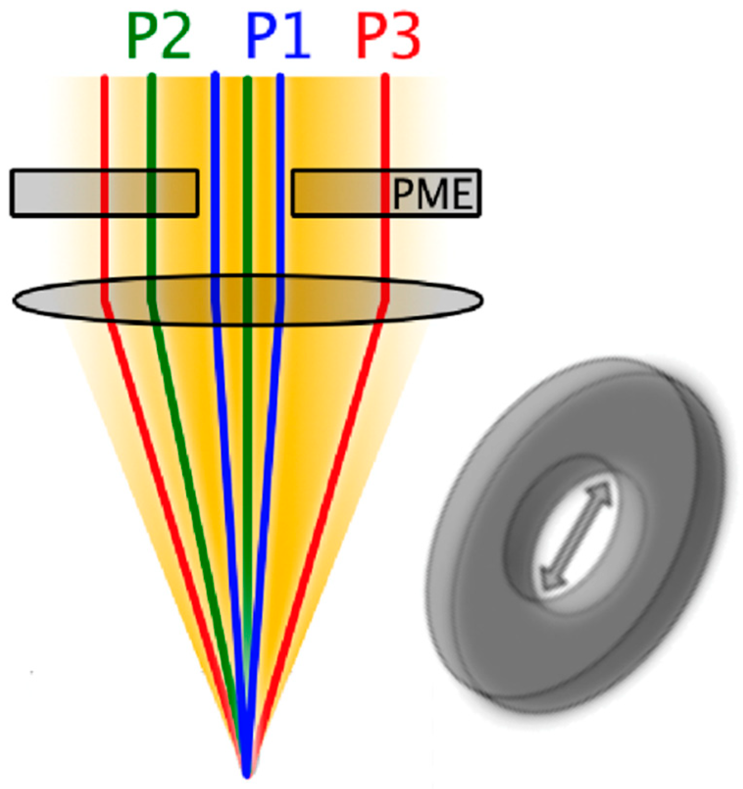
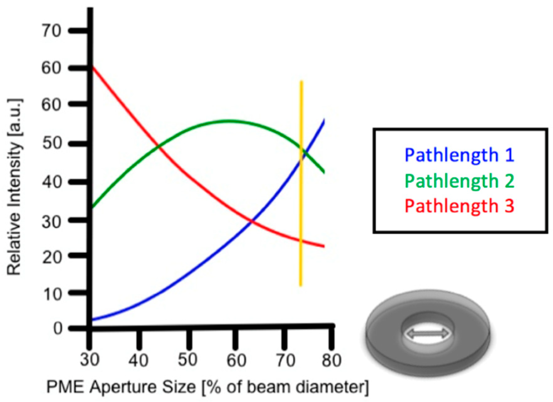
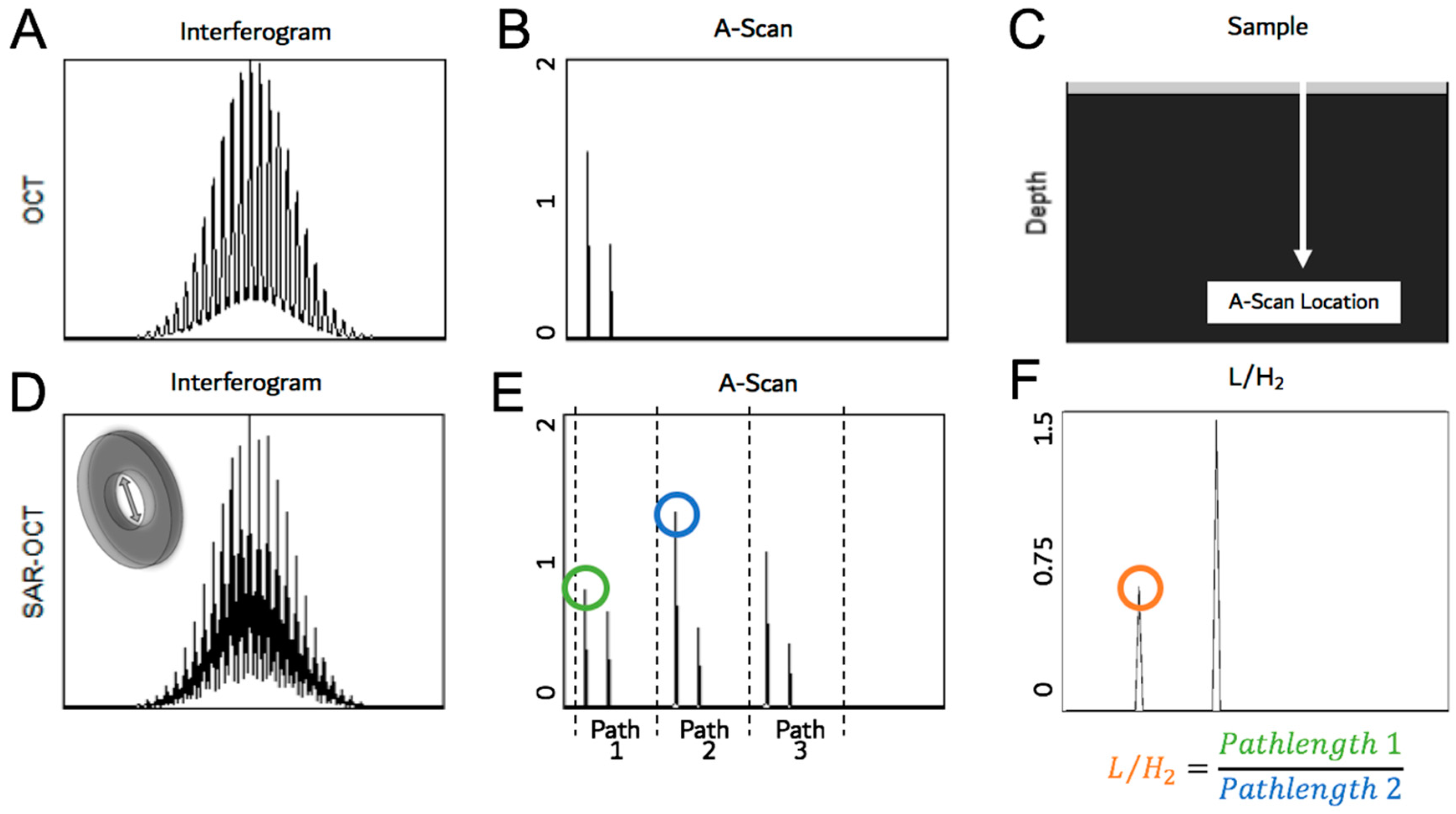
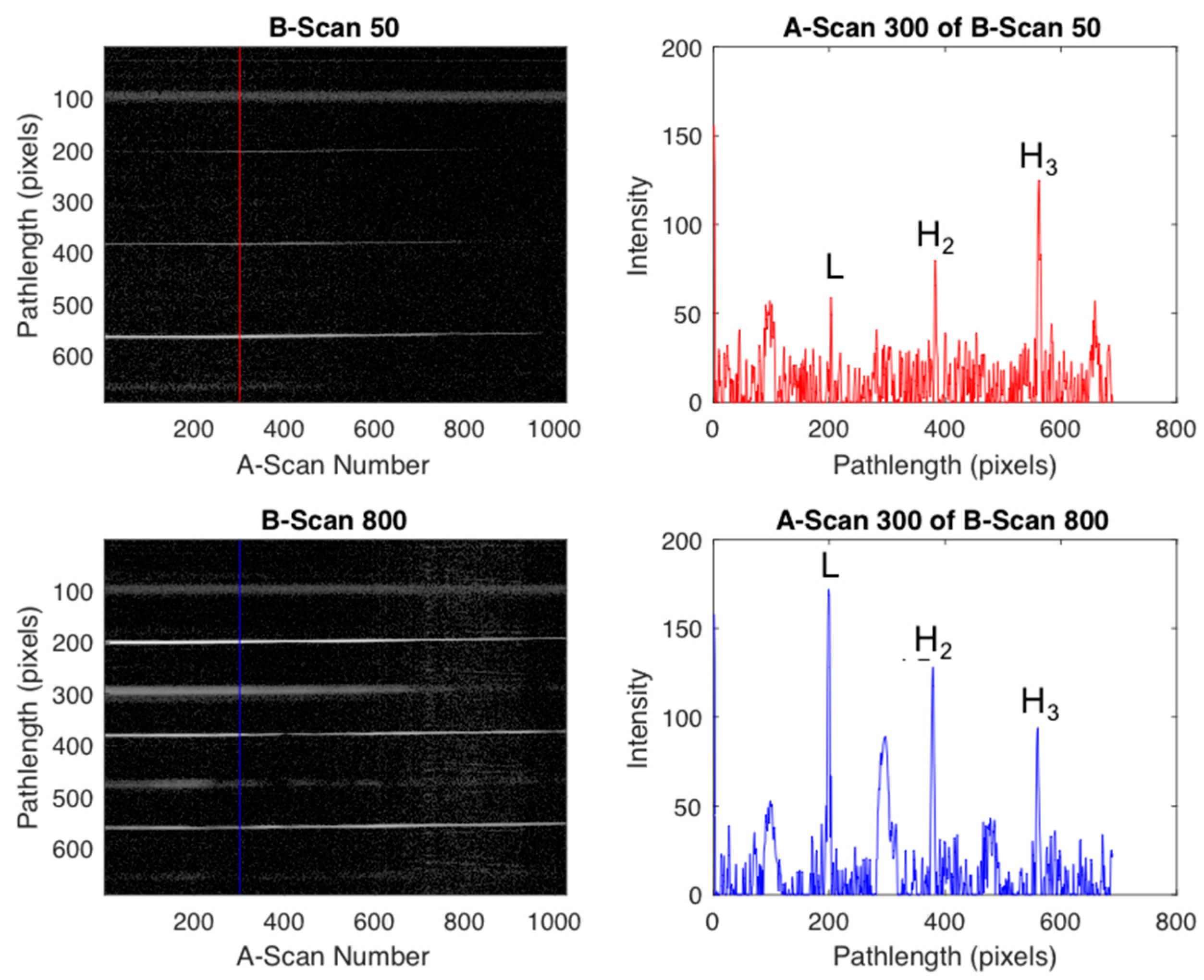
2.2.5. Pathlength Multiplexing Element

An important component to the SAR-OCT system is the pathlength multiplexing element (PME). The PME is a BK7 window, 5 mm thick, with a central clear aperture. The center aperture has a 7 mm diameter. Light in the sample arm of the SAR-OCT system has three potential optical pathlengths: Pathlength 1 is light that travels through the center aperture to and from the retina. Pathlength 2 is light that travels through the PME central aperture once—to or from the retina. Pathlength 3 is light that does not travel through the PME central aperture—to and from the retina. Figure 3 illustrates the three pathlengths.

Mathematically, the additional pathlengths added for each path through any PME are described generally below:

Additional pathlength added for Pathlength 1 ($L_L$) is

$$L_L = \left(d+d\right)-\left(d+d\right) = 0.$$

(3)

Additional pathlength added for Pathlength 2 ($L_{H2}$) is

$$L_{H2} = \left(d+n·d\right)-\left(d+d\right) = d\left(n-1\right).$$

(4)

Additional pathlength added for Pathlength 3 ($L_{H3}$) is

$$L_{H3} = \left(n·d+n·d\right)-\left(d+d\right) = 2d\left(n-1\right).$$

(5)

In Equations (3)–(5), d is the physical PME thickness, and n is refractive index of the glass at the center wavelength of the OCT system. For the 5 mm thick BK7 PME (n = 1.50 at 1310 nm), $L_L$ = 0, $L_{H2}$ = 2.5 mm, and $L_{H3}$ = 5 mm. Thus, each sub image in the OCT interferogram is separated vertically by 2.5 mm. A more rigorous Fourier optical analysis of the PME operation for imaging was previously published [33].

A Monte Carlo model was developed to determine the effect of PME center aperture size on the intensity of light in each pathlength. Photons were randomly generated within the beam area, and each photon was weighted by its position in the Gaussian beam profile of the OCT source. Then, each photon was assigned a scattering angle off of the sample based on an assigned g-factor (anisotropy) of 0.97, a measured g anisotropy value for the neural retina [34]. The Monte Carlo simulation recorded whether the photon travelled through the PME glass once, twice, or never, and each photon contributed to the intensity of its assigned pathlength (Figure 4). The scattering angle of the photon was also recorded. The results of the Monte Carlo simulation suggested no single PME aperture size exists at which the pathlength intensities are equal.

Plotting the angular distribution of backscattered photons for each pathlength revealed that Pathlengths 1 and 2 have greatest angular discrimination (Figure 5). Pathlength 3 contains light that is scattered at each extreme—both direct backscattering and high-angle backscattering. This simulation relative PME intensities in Figure 4. To maximize utility of the angular discrimination in Pathlengths 1 and 2, a PME aperture size was selected around 72% of the beam diameter. At this aperture size, the intensities of light in Pathlengths 1 and 2 were about equal, while the intensity of light in Pathlength 3 was about half that of Pathlengths 1 and 2. This selection is indicated by the yellow line in Figure 4, and the angular distribution of light at this aperture size is plotted in Figure 5.

Given the 12 mm beam diameter after the reflective collimator (Figure 1) and available discrete drill bit sizes, a 7 mm diameter central aperture was selected for the PME.

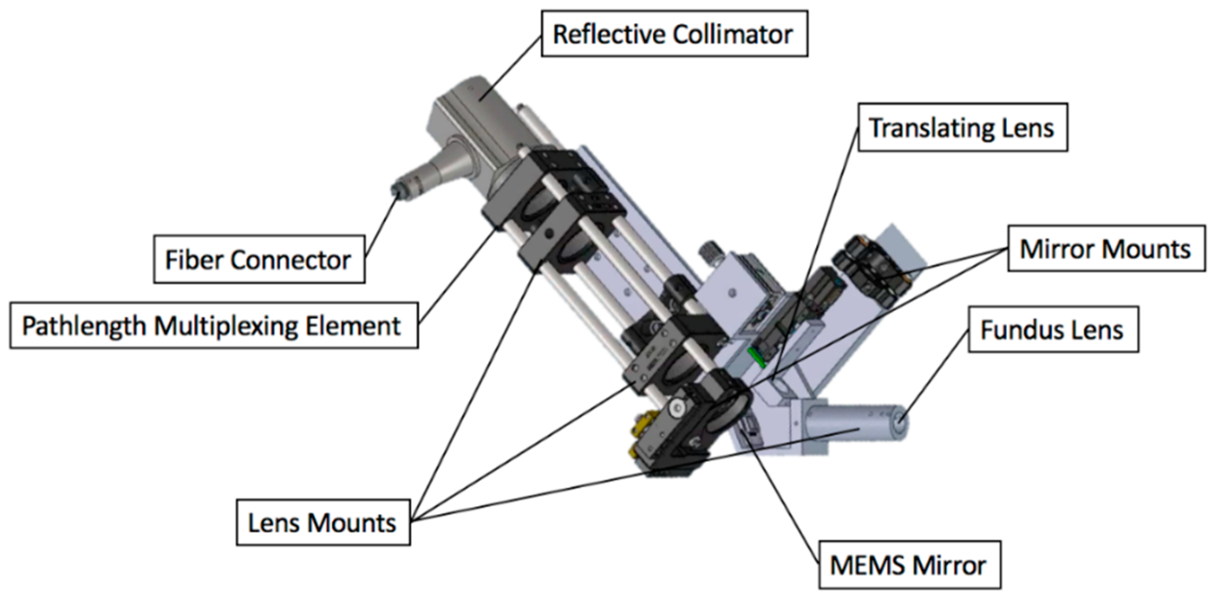
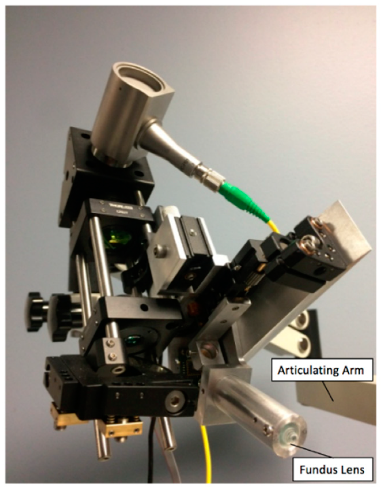
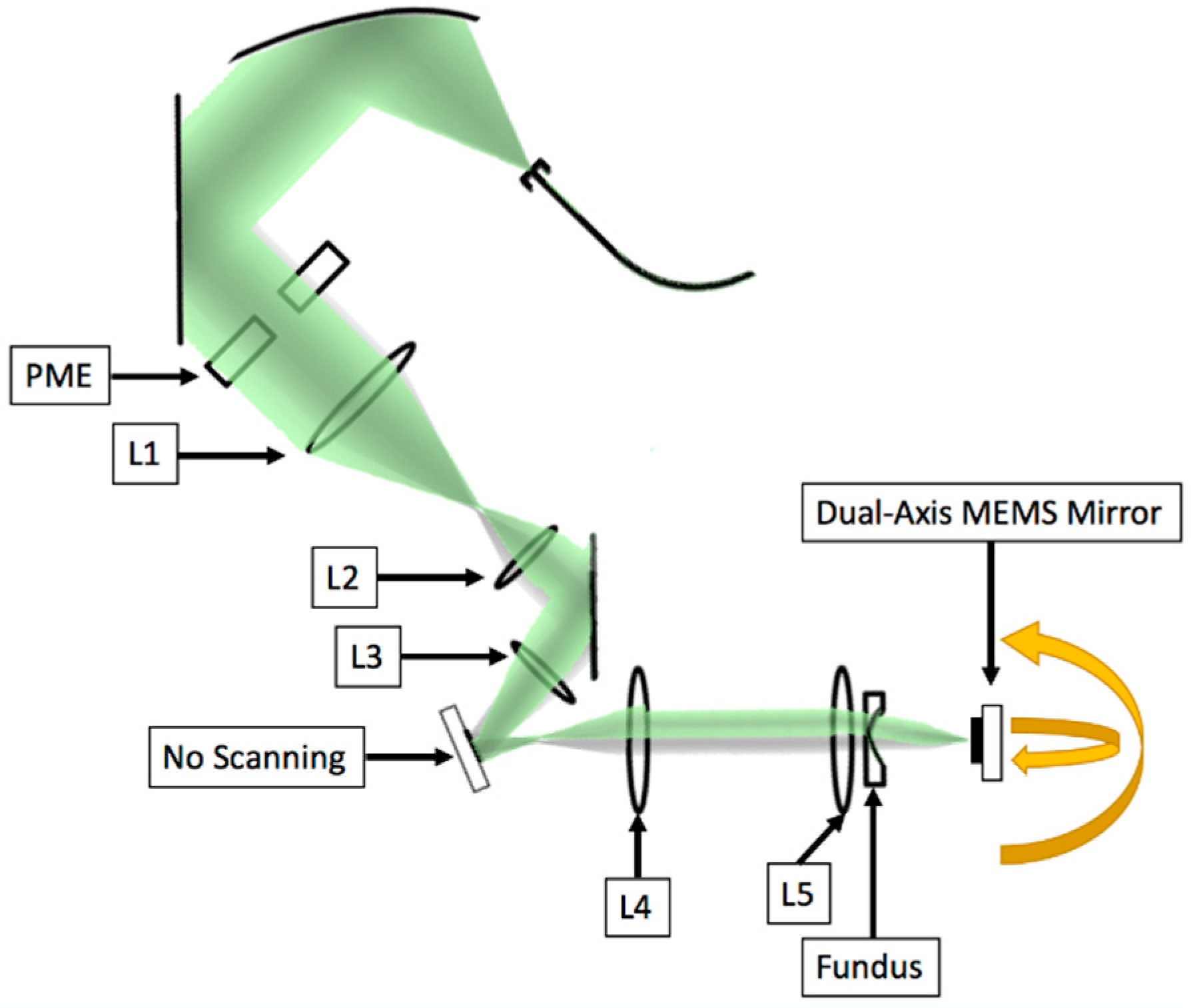
2.2.6. System Construction

Since the system must be transportable to and from the operating room for imaging mice under anesthesia, the SAR-OCT system was designed to be mounted on an articulating arm, which was mounted on a rolling cart. To fit the arm, the system needed to be compact and stable, yet flexible enough to allow for adjusting high-precision optical components. The SAR-OCT mechanical system was custom-designed in a computer aided design (CAD) software package with a combination of off-the-shelf optical components (ThorLabs) and custom aluminum components for mounting optics. Aluminum parts were machined by the University of Texas at Austin’s Mechanical Engineering machine shop. A complete CAD rendering of the SAR-OCT design is pictured in Figure 6, and a photo of the constructed system is in Figure 7.

2.3. System Characterization

After designing the system, experiments were conducted to verify imaging performance of the SAR-OCT system. These involved scattering angle characterization and finally, murine retinal imaging.

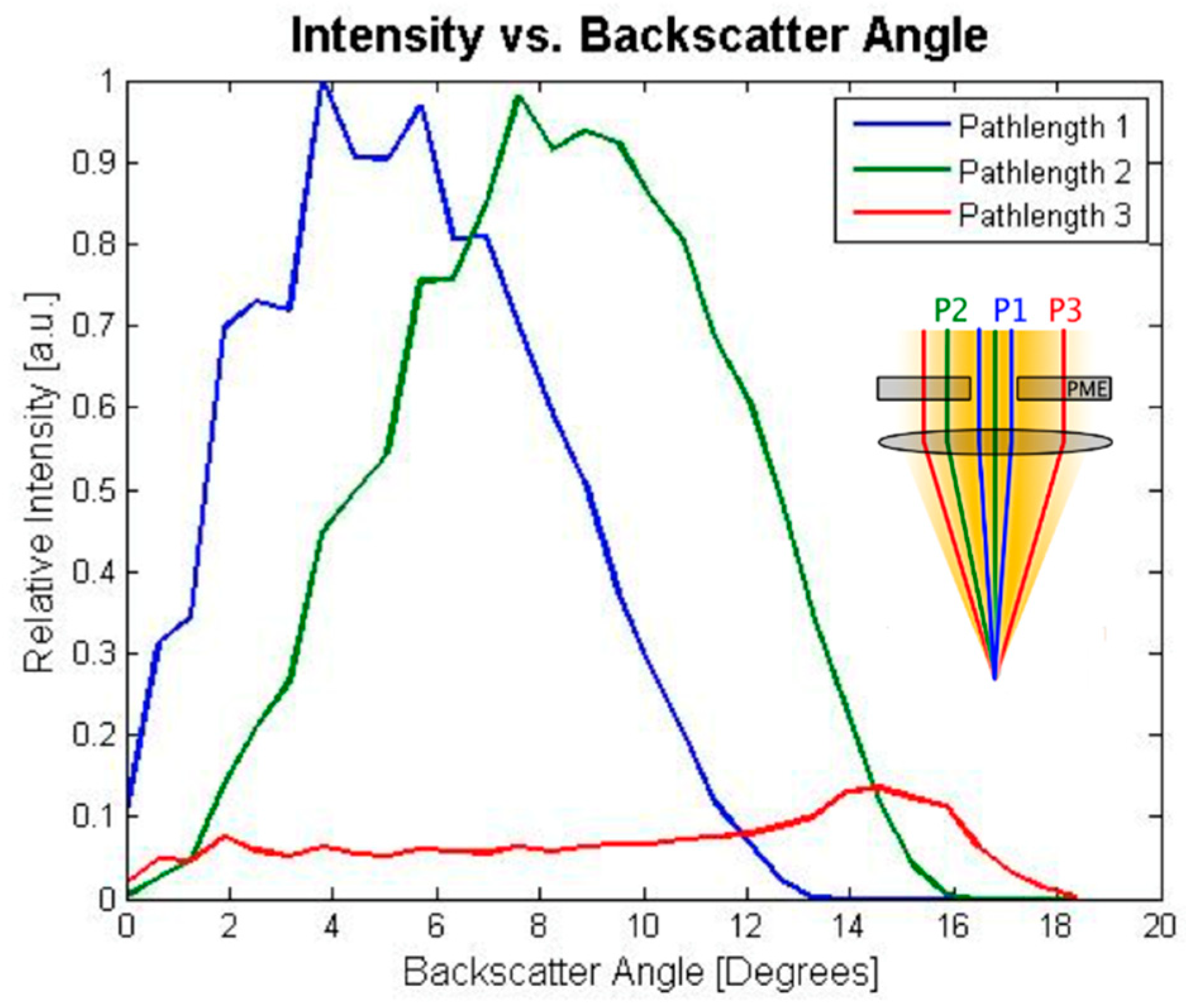
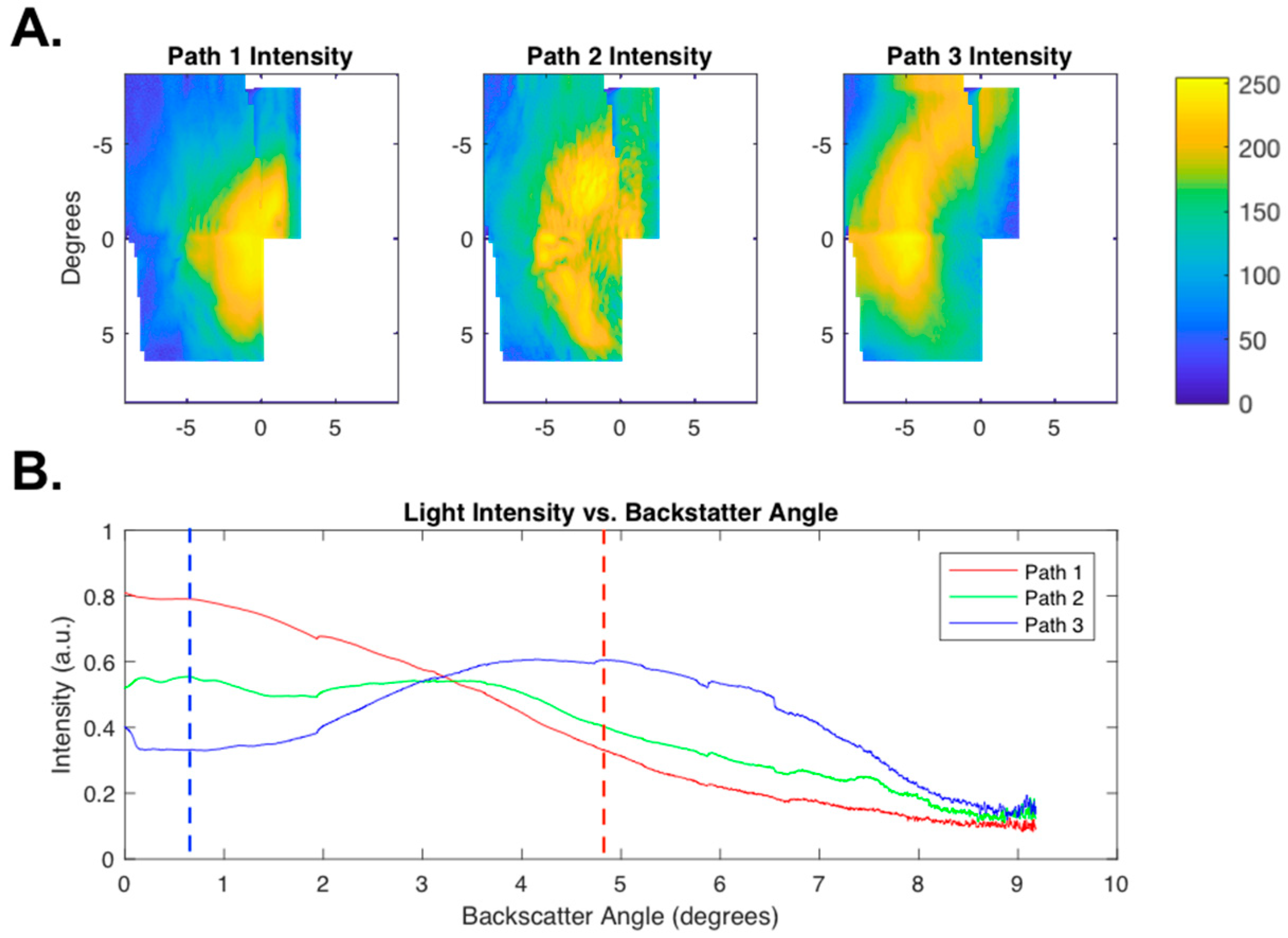
2.3.1. Scattering Angle Characterization

To characterize system’s sensitivity to changes in scattering angle, an experiment was designed in which light was reflected back at known angles. The dual-axis MEMS mirror was placed just beyond the focal plane of the objective lens and raster-scanned to collect a range of pathlength intensities corresponding to bulk scattering angles (Figure 8). The incident beam was not scanned in this configuration, only the angle at which the light was reflected from the dual-axis MEMS mirror in the focal plane. Orientation of the dual-axis MEMS mirror varied by ±4 degrees in the x- and y-directions; thus, several raster scans were collected with various tilt offsets and stitched together in post-processing.

Depths corresponding to the MEMS mirror at Pathlengths 1–3 were isolated, and then intensity values corresponding to a given reflection angle were averaged azimuthally in reference to the neutral position (degree 0,0). Results are given in Section 3.2.

2.3.2. Imaging Protocol

Murine retinal images were recorded using the SAR-OCT system (IACUC protocol: #AUP-2015-00156) and the total intensities in each pathlength for 32 mice (B6SJL F1/J—JAX #100012) were recorded. The intensities were normalized to the pathlength with the maximum intensity. The relative intensities in Pathlengths 1–3 were compared to the results of the Monte Carlo model to assess the agreement between the model and the imaging system.

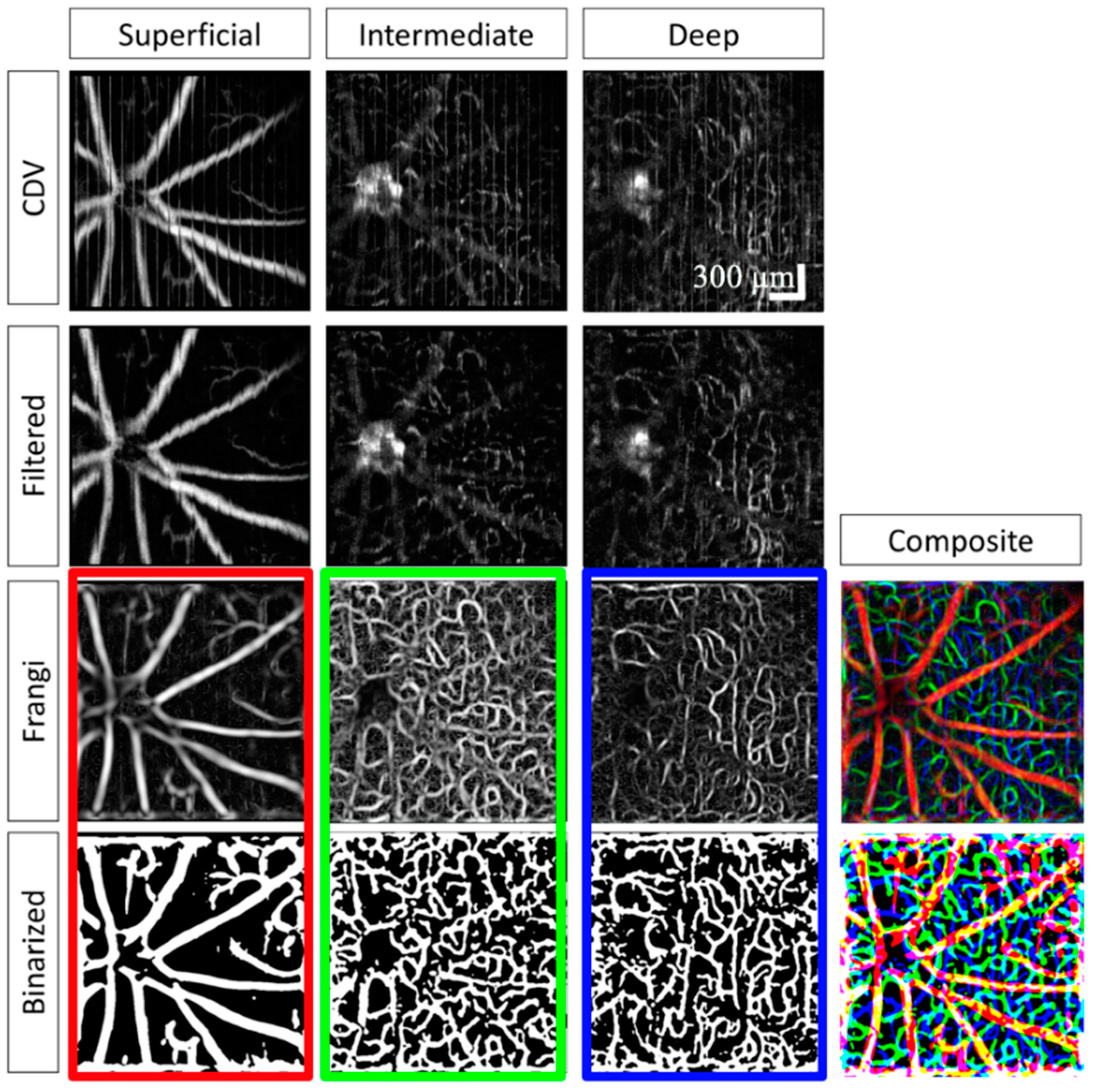
2.4. Image Processing

2.4.1. Initial Processing

With inclusion of the PME, three sub-images are observed in every B-scan, each corresponding to three different bulk scattering angles. To align the images for analysis, the first sub-image (Pathlength 1) is used as a reference. Sub-images are selected manually, each with the same height (typically ~150 pixels). Then, Pathlengths 2 and 3 are shifted in the z-direction (axially) to align with Pathlength 1. The MATLAB function “imregister” is set to perform only axial shifting for precise alignment. Simple axial shifting, in contrast to other more complex methods, is appropriate for this system because it is known a priori that each A-scan location contains the exact same retinal cross section in the three sub-images. Any image registration that goes beyond simple axial shifting risks mixing A-scans across different locations and corrupting the scattering angle analysis. After the sub-images are aligned, each pathlength sub-image is saved as a tiff stack. This results in three image stacks with size 150 (height) × 512 (width) × 4096 (depth). These image stacks are stored without any image compression to maintain signal fidelity.

This first initial processing step outputs three aligned image stacks. With these three stacks, intensity processing, speckle processing, and segmentation may be performed before the four subsequent analysis steps for feature extraction.

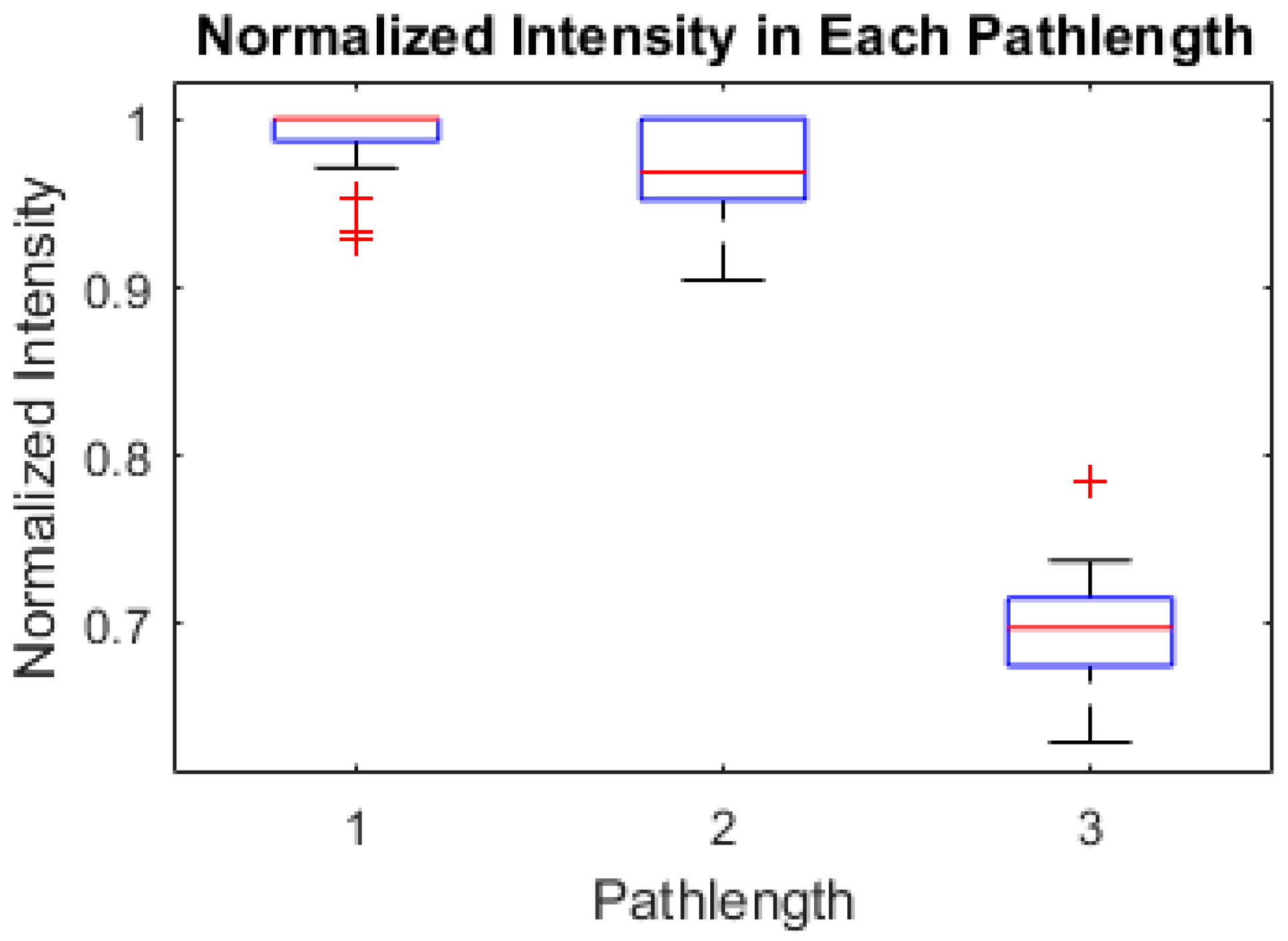
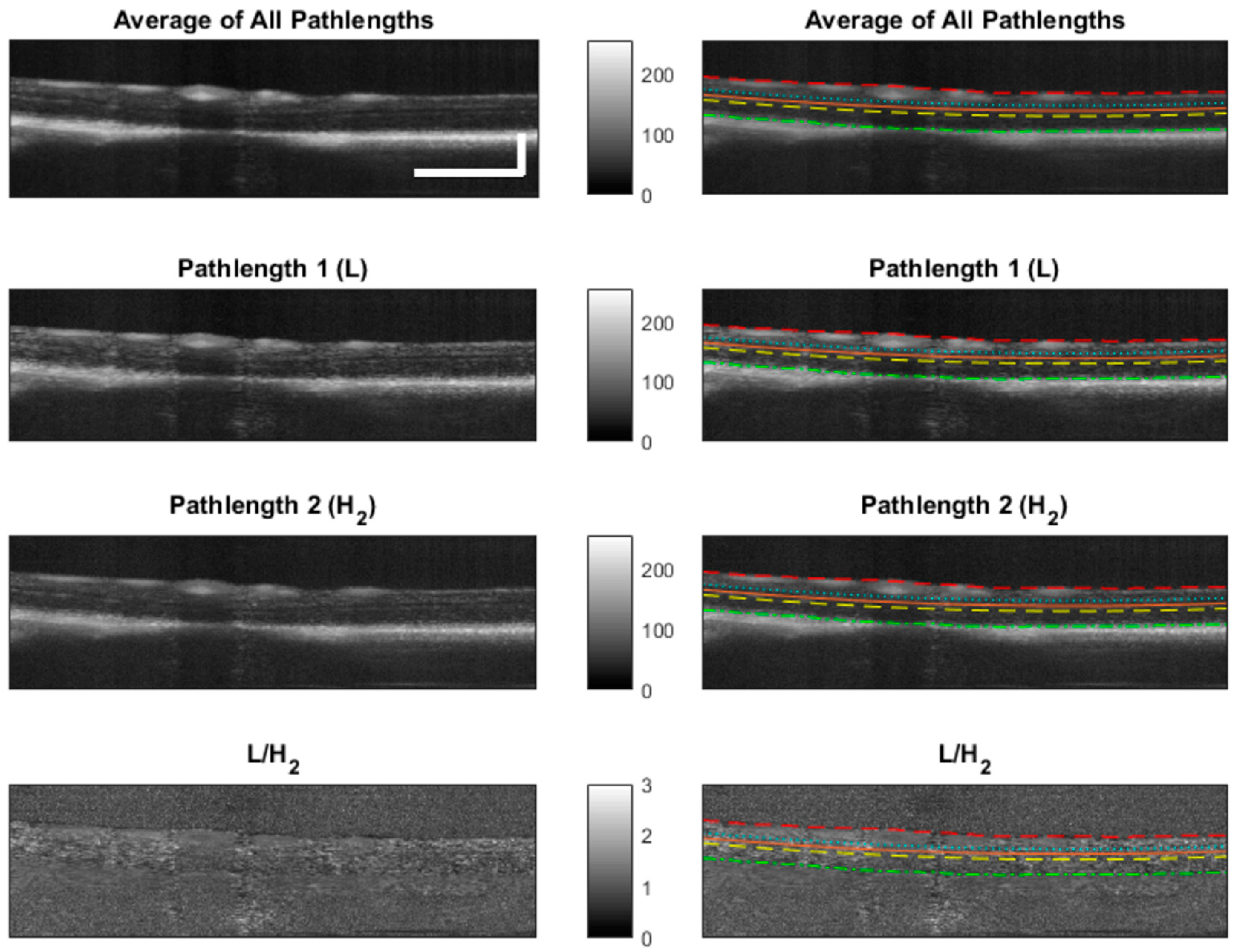
2.4.2. Intensity Processing

Before analysis can be performed, eight repeating B-scans in each B-scan location are first averaged together and collapsed into one B-scan. Thus, the three sub-images previously aligned and saved are taken from size 150 × 512 × 4095 to 150 × 512 × 512. Averaging over the eight repeated B-scans yields higher signal-to-noise ratios (SNR). These three volumes, corresponding to each of the three pathlengths, are later used in scattering angle analysis.

The second process under intensity processing is to average the three sub-images (150 × 512 × 512) voxel-by-voxel. Averaging further increases SNR and permits more repeatable analysis of layer thickness and reflectance index.

2.4.3. Speckle Processing

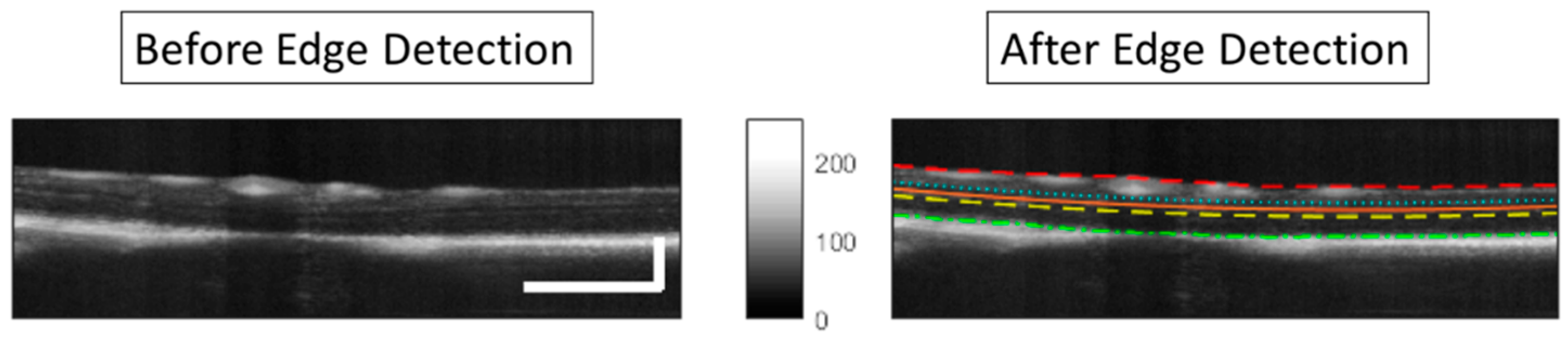
Several established methods exist to determine areas of blood flow using OCT for biomedical imaging. One approach is complex differential variance (CDV), which intrinsically limits phase noise due to bulk motion [35]. Because of its outperformance of other methods based on angiographic analysis of collected SAR-OCT retinal images, CDV was selected as the angiographic method for this SAR-OCT device.

The CDV signal for any given A-scan can be described as

$$f_{CDV}\left(z\right) = \sqrt{1-\frac{{\sum }_{t = 1}^{M-1}\left|{\sum }_{k = -L}^{L}w\left(k\right)R\left(z-k,t\right)R^{*}\left(z-k,t+1\right)\right|}{{\sum }_{t = 1}^{M-1}{\sum }_{K = -L}^{L}w\left(k\right)\frac{1}{2}[{\left|R\left(z-k,t\right)\right|}^2+{\left|R\left(z-k,t+1\right)\right|}^2]}},$$

(6)

where M is the total number of repeating B-scans, L (more precisely, 2L + 1) is the length of the kernel, w is the depth window function, and R is the complex analytic OCT signal at time point t (R = A(z,t)e^iφ(z,t)). The coherent average is normalized by division with the incoherent average of the original A-scan data.

Three sequential processes take CDV volumes as input to obtain high-fidelity angiograms: (1) filtering to remove bulk motion; (2) Frangi vesselness filter to improve SNR; and (3) adaptive thresholding for binarizing angiograms.

Despite the CDV algorithm’s robustness compared to other methods, the problem of bulk motion can still be observed such that vertical lines obscure vascular structures. These vertical lines are due to bulk movements of the mouse including heart beat and breathing. For filtering to remove bulk motion artifacts, these lines are first detected manually, with the user clicking to the left and right of a line in the superficial plexus image. The width of the line is then determined by a custom MATLAB script, and the entire artifact is replaced with values taken from the left and right of the obscuring line. The same replacement process is repeated automatically in the intermediate and deep plexuses.

The second filtering process applies the Frangi vesselness filter [36] to the filtered image to isolate those areas of the image that are vessel-like. The Frangi filter, which uses Gaussian-like distributions with user-defined widths to search for vessel-like features, is a helpful tool for the retina because the sizes of the vessels are generally known, a priori. The Frangi filter takes as inputs the size distribution of vessels and searches for structures that are around that size. A range of three sigma values suited the vessel size distribution are selected. Additional Frangi parameters included β₁ (0.5) and β₂ (5). If not handled judiciously, Frangi filtering could introduce false vessel structures from noise.

The final step was to binarize image such that more intensive vascular analysis could be performed. The image was binarized using a built-in MATLAB filter with adaptive thresholding. One note here is that adaptive filtering assumes the presence of a vessel.

2.4.4. Segmentation

The murine retinal segmentation algorithm for the SAR-OCT images used here can be characterized as three kinds of processes interspersed throughout the algorithm: (1) stack conditioning; (2) Sobel edge detection; and (3) error removal, each custom-designed in MATLAB.

As a part of the stack conditioning process, the angiography and intensity scans are simply summed. Because the vasculature of the murine retina is highly localized to particular regions, the addition of SAR-OCT intensity volume with the angiography image intensifies the boundaries between retinal layers.

Another part of the stack conditioning process occurs after detection of the ONL/RPE boundary. The retina is flattened with reference to the ONL/RPE boundary. Then, a median filter is applied (50 × 50 × 1 voxels). Because the retina has been flattened, this process works to provide some uniformity within each layer and present retinal layers more distinct.

The second category of segmentation is edge detection. Each boundary is determined by examining volumes that have been filtered with a Sobel edge detection filter [37]. The Sobel filter has a convolution kernel given by:

$$\left[ \begin{array}{ccc}-1& -2& 1\\ 0& 0& 0\\ 1& 2& 1\end{array} \right].$$

The ONL/RPE boundary is, for the most part, the most prominent edge detected by the Sobel filter. However, spurious noise could also be detected by the filter, thus a secondary means of eliminating wrong boundaries was employed. Before the edge is selected by the MATLAB script, the user of the script must manually click throughout the image over several boundaries as prompted by the script. The user input is used as an initial guess for boundary detection; that is, boundaries are only considered as the possible correct boundary if they are within a physiologically reasonable range of the inputted boundary. This clicking technique is applied to three of the five boundaries detected: the ONL/RPE, INL/OPL and the vitreous/ILM boundaries.

Finally, inputs of these user inputs are also used to form a 3D second-order polynomial that is utilized in the third processing step, error removal. Occasionally as edge selected by the MATLAB script is incorrect, and, perhaps, the edge is not even reasonably determinable by the human eye. In such cases, edge location is estimated based on the surrounding tissues (e.g., under vessel shadows). In these cases, the 3D polynomial is manually selected (in those regions alone) to replace the semi-automatically detected edges.

2.4.5. Scattering Angle Feature

Ratio processing is the simplest approach to leveraging the utility of SAR-OCT, and is the approach previously described by Wang et al. [31]. Wang looked to Pathlength 3 as it contains the highest possible scatterers and found that the ratio of Pathlength 1 to Pathlength 3 (L/H₃) correlated with known azimuthal variation of retinal ganglion cell size.

However, as was demonstrated in the Monte Carlo simulation, Pathlength 2 and Pathlength 1 provide the greatest angular discrimination. Although Pathlength 3 contains higher backscattering angles than Pathlength 2, Pathlength 3 also contains the lowest possible angles (direct backscattering). Thus, L/H₂ was decided upon as an image feature. A visual explanation of the PME and L/H₂ is provided in Figure 9.

3. Results and Discussion

3.1. Mouse Eye Optics

Combined, the radii of curvature and refractive indices for each murine eye segment (

Table 2. Conrady parameters for the murine ocular media.

Eye Segment	n0	B	C	n (at 1.31 µm)	RMS Error
Cornea	1.399	−2.177 × 10−3	1.260 × 10−3	1.398	1.674 × 10-4
Aqueous	1.289	3.277 × 10−2	−1.382 × 10−3	1.313	1.834 × 10-4
Lens	1.635	2.831 × 10−3	4.411 × 10−3	1.639	2.567 × 10-4
Vitreous	1.319	8.008 × 10−3	2.551 × 10−4	1.326	1.228 × 10−4

) yielded a suitable optical model in OpticStudio (Zemax). Figure 10 shows a real mouse eye cross section from Remtalluh superimposed with the optical model described above.

3.2. Scattering Angle Characterization

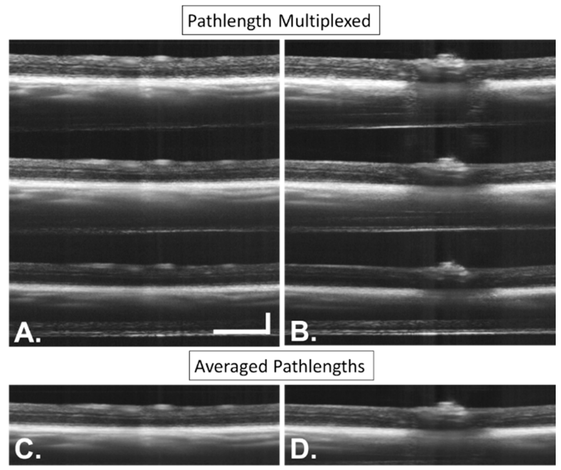
Figure 11 shows sample B-scans from the scattering angle characterization experiment. Figure 12A shows the intensity of each pathlength for each angular displacement, and Figure 12B plots the intensities after azimuthal averaging. The sample A-scans (Figure 11) are also indicated in the same color by vertical dashed lines in Figure 12B.

Experimental results determined that the SAR-OCT murine retinal imaging system can detect changes in bulk scattering angle up to eight degrees from a direct backscatter. That is, from a zero-degree backscattering angle to an eight-degree backscattering angle, the combination of light from Pathlengths 1–3 have unique contributions to the total image intensity. Light scattered from a sample at an angle greater than eight degrees is not recorded by the SAR-OCT system.

3.3. Imaging

Based on the Monte Carlo model results (Figure 4 and Figure 5), light intensities in Pathlengths 1 and 2 are expected to be about equal, and the intensity of light in Pathlength 3 should be about 50% of that in Pathlengths 1 and 2. Light intensities in Pathlengths 1 and 2 were not statistically different, but the experimental results also show a greater intensity of light in Pathlength 3 than the Monte Carlo simulation predicted (Figure 5 and Figure 13). Nevertheless, this increase in Pathlength 3 intensity (compared to the simulation results) is beneficial because greater balance among the pathlengths yields higher quality composite images and a greater dynamic range for scattering angle analysis. Sample SAR-OCT images are also shown in Figure 14.

3.4. Image Processing

Example angiography results and edge detection results are shown in Figure 15 and Figure 16. With angiography and edge detection, the scattering angle indices can be categorized by vascular zone or retinal layer.

To obtain a L/H₂ tomogram, Pathlengths 1 and 2 are divided at every voxel position. With this approach, the segmentation output can be superimposed on the volume to sort the retinal L/H₂ values into their corresponding layers (Figure 17).

4. Conclusions

A simple mouse eye optical model at a wavelength 1.3 µm is introduced for the first time. This model informed SAR-OCT system design. Extensive design analysis and performance characteristics are presented for murine retinal imaging system, including laser and fiber optic components, the 2D MEMS mirror for beam scanning, the value of corneal contact for mouse eye imaging, dispersion compensation, PME computational modeling, and system construction. Image processing techniques are described in relation to unique SAR-OCT demands, including intensity processing, angiography, and retinal segmentation. Finally, the results of the analysis are presented in murine eye. The reported SAR-OCT system is shown to be sensitive to angular scattering up to eight degrees off normal. Example B-scans of mouse retinas, angiography images, and retinal segmentation results are presented to demonstrate the capacity of SAR-OCT to maintain retinal imaging fidelity, similar to that of other reported devices, while also adding the contrast mechanism due to scattering angle. Using a SAR-OCT imaging device such as the one described here enables new methods of scattering angle analysis for animal disease models that affect the morphology of biological structures in the retina, such as Alzheimer’s disease, glaucoma, and traumatic encephalopathy.

References

1. Huang, D.; Swanson, E.A.E.A.; Lin, C.P.C.P.; Schuman, J.S.; Stinson, W.G.; Chang, W.; Hee, M.R.; Flotte, T.; Gregory, K.; Puliafito, C.A.; et al. Optical Coherence Tomography. Science 1991, 254, 1178–1181. [Google Scholar] [CrossRef] [PubMed]
2. Fujimoto, J.G. Optical Coherence Tomography for Retinal Imaging. Biomed. Photonics Handb. 2003, 4, 402–403. [Google Scholar] [CrossRef]
3. Wilson, J.D.; Bigelow, C.E.; Calkins, D.J.; Foster, T.H. Light Scattering from Intact Cells Reports Oxidative-Stress-Induced Mitochondrial Swelling. Biophys. J. 2005, 88, 2929–2938. [Google Scholar] [CrossRef] [PubMed] [Green Version]
4. Boustany, N.N.; Drezek, R.; Thakor, N.V. Calcium-Induced Alterations in Mitochondrial Morphology Quantified in Situ with Optical Scatter Imaging. Biophys. J. 2002, 83, 1691–1700. [Google Scholar] [CrossRef] [Green Version]
5. Pasternack, R.M.; Zheng, J.-Y.; Boustany, N.N. Optical scatter changes at the onset of apoptosis are spatially associated with mitochondria. J. Biomed. Opt. 2010, 15, 040504. [Google Scholar] [CrossRef] [PubMed] [Green Version]
6. Boustany, N.N.; Tsai, Y.-C.; Pfister, B.; Joiner, W.M.; Oyler, G.A.; Thakor, N.V. BCL-xL-dependent light scattering by apoptotic cells. Biophys. J. 2004, 87, 4163–4171. [Google Scholar] [CrossRef] [PubMed]
7. Beauvoit, B.; Evans, S.M.; Jenkins, T.W.; Miller, E.E.; Chance, B. Correlation between the light scattering and the mitochondrial content of normal tissues and transplantable rodent tumors. Anal. Biochem. 1995, 226, 167–174. [Google Scholar] [CrossRef] [PubMed]
8. Kim, S.; Heflin, S.; Kresty, L.A.; Halling, M.; Perez, L.N.; Ho, D.; Crose, M.; Brown, W.; Farsiu, S.; Arshavsky, V.; et al. Analyzing spatial correlations in tissue using angle-resolved low coherence interferometry measurements guided by co-located optical coherence tomography. Biomed. Opt. Express 2016, 7, 1400–1414. [Google Scholar] [CrossRef] [PubMed]
9. Wax, A.; Yang, C.; Backman, V.; Badizadegan, K.; Boone, C.W.; Dasari, R.R.; Feld, M.S. Cellular Organization and Substructure Measured Using Angle-Resolved Low-Coherence Interferometry. Biophys. J. 2002, 82, 2256–2264. [Google Scholar] [CrossRef] [Green Version]
10. Dwelle, J.; Liu, S.; Wang, B.; McElroy, A.; Ho, D.; Markey, M.K.; Milner, T.; Rylander, H.G., 3rd; Grady Rylander, H. Thickness, phase retardation, birefringence, and reflectance of the retinal nerve fiber layer in normal and glaucomatous non-human primates. Investig. Ophthalmol. Vis. Sci. 2012, 53, 4380–4395. [Google Scholar] [CrossRef] [PubMed]
11. Liu, S.; Wang, B.; Yin, B.; Milner, T.E.; Markey, M.K.; McKinnon, S.J.; Rylander, H.G., III. Retinal nerve fiber layer reflectance for early glaucoma diagnosis. J. Glaucoma 2014, 23, 45–52. [Google Scholar] [CrossRef] [PubMed]
12. Wang, B.; Yin, B.; Dwelle, J.; Rylander, H.G.; Markey, M.K.; Milner, T.E. Path-length-multiplexed scattering-angle-diverse optical coherence tomography for retinal imaging. Opt. Lett. 2013, 38, 4374–4377. [Google Scholar] [CrossRef] [PubMed]
13. Wartak, A.; Augustin, M.; Haindl, R.; Beer, F.; Salas, M.; Laslandes, M.; Baumann, B.; Pircher, M.; Hitzenberger, C.K. Multi-directional optical coherence tomography for retinal imaging. Biomed. Opt. Express 2017, 8, 5560–5578. [Google Scholar] [CrossRef] [PubMed]
14. Wartak, A.; Haindl, R.; Trasischker, W.; Baumann, B.; Pircher, M.; Hitzenberger, C.K. Active-passive path-length encoded (APPLE) Doppler OCT. Biomed. Opt. Express 2016, 7, 5233–5251. [Google Scholar] [CrossRef] [PubMed]
15. Geng, Y.; Schery, L.A.; Sharma, R.; Dubra, A.; Ahmad, K.; Libby, R.T.; Williams, D.R. Optical properties of the mouse eye. Biomed. Opt. Express 2011, 2, 717–738. [Google Scholar] [CrossRef] [PubMed] [Green Version]
16. Remtulla, S.; Hallett, P.E. A schematic eye for the mouse, and comparisons with the rat. Vis. Res. 1985, 25, 21–31. [Google Scholar] [CrossRef]
17. Schmucker, C.; Schaeffel, F. A paraxial schematic eye model for the growing C57BL/6 mouse. Vis. Res. 2004, 44, 1857–1867. [Google Scholar] [CrossRef] [PubMed]
18. Conrady, A.E. Applied Optics and Optical Design, Part Two, 1st ed.; Kingslake, R., Ed.; Dover Publications, Inc.: New York, NY, USA, 1960. [Google Scholar]
19. Gardner, M.R.; Katta, N.; McElroy, A.; Baruah, V.; Rylander, H.G.; Milner, T.E. Scattering angle resolved optical coherence tomography for in vivo murine retinal imaging. In SPIE BiOS; International Society for Optics and Photonics: San Franscisco, CA, USA, 2017; p. 100531O. [Google Scholar]
20. Swanson, E.A.; Izatt, J.A.; Lin, C.P.; Fujimoto, J.G.; Schuman, J.S.; Hee, M.R.; Huang, D.; Puliafito, C.A. In vivo retinal imaging by optical coherence tomography. Opt. Lett. 1993, 18, 1864–1866. [Google Scholar] [CrossRef] [PubMed]
21. Carrasco-Zevallos, O.; Nankivil, D.; Keller, B.; Viehland, C.; Lujan, B.J.; Izatt, J.A. Pupil tracking optical coherence tomography for precise control of pupil entry position. Biomed. Opt. Express 2015, 6, 3405–3419. [Google Scholar] [CrossRef] [PubMed] [Green Version]
22. Kumar, K.; Condit, J.C.; McElroy, A.; Kemp, N.J.; Hoshino, K.; Milner, T.E.; Zhang, X. Fast 3D in vivo swept-source optical coherence tomography using a two-axis MEMS scanning micromirror. J. Opt. A Pure Appl. Opt. 2008, 10, 044013. [Google Scholar] [CrossRef]
23. Aguirre, A.D.; Herz, P.R.; Chen, Y.; Fujimoto, J.G.; Piyawattanametha, W.; Fan, L.; Wu, M.C. Two-axis MEMS scanning catheter for ultrahigh resolution three-dimensional and en face imaging. Opt. Express 2007, 15, 2445–2453. [Google Scholar] [CrossRef] [PubMed]
24. Lu, C.D.; Kraus, M.F.; Potsaid, B.; Liu, J.J.; Choi, W.; Jayaraman, V.; Cable, A.E.; Hornegger, J.; Duker, J.S.; Fujimoto, J.G. Handheld ultrahigh speed swept source optical coherence tomography instrument using a MEMS scanning mirror. Biomed. Opt. Express 2014, 5, 293–311. [Google Scholar] [CrossRef] [PubMed]
25. LaRocca, F.; Nankivil, D.; DuBose, T.; Toth, C.A.; Farsiu, S.; Izatt, J.A. In vivo cellular-resolution retinal imaging in infants and children using an ultracompact handheld probe. Nat. Photonics 2016, 10, 580–584. [Google Scholar] [CrossRef] [PubMed] [Green Version]
26. De la Cera, E.G.; Rodríguez, G.; Llorente, L.; Schaeffel, F.; Marcos, S. Optical aberrations in the mouse eye. Vis. Res. 2006, 46, 2546–2553. [Google Scholar] [CrossRef] [PubMed]
27. Yu, Y.; Zhang, T.; Meadway, A.; Wang, X.; Zhang, Y. High-speed adaptive optics for imaging of the living human eye. Opt. Express 2015, 23, 23035–23052. [Google Scholar] [CrossRef] [PubMed] [Green Version]
28. Zawadzki, R.J.; Jones, S.M.; Olivier, S.S.; Zhao, M.; Bower, B.A.; Izatt, J.A.; Choi, S.; Laut, S.; Werner, J.S. Adaptive-optics optical coherence tomography for high-resolution and high-speed 3D retinal in vivo imaging. Opt. Express 2005, 13, 8532–8546. [Google Scholar] [CrossRef] [PubMed]
29. Jian, Y.; Xu, J.; Gradowski, M.A.; Bonora, S.; Zawadzki, R.J.; Sarunic, M.V. Wavefront sensorless adaptive optics optical coherence tomography for in vivo retinal imaging in mice. Biomed. Opt. Express 2014, 5, 547–559. [Google Scholar] [CrossRef] [PubMed]
30. Jian, Y.; Zawadzki, R.J.; Sarunic, M.V. Adaptive optics optical coherence tomography for in vivo mouse retinal imaging. J. Biomed. Opt. 2013, 18, 056007. [Google Scholar] [CrossRef] [PubMed] [Green Version]
31. Liu, X.; Wang, C.-H.; Dai, C.; Camesa, A.; Zhang, H.F.; Jiao, S. Effect of Contact Lens on Optical Coherence Tomography Imaging of Rodent Retina. Curr. Eye Res. 2013, 38, 997–1003. [Google Scholar] [CrossRef] [PubMed]
32. Zhang, P.; Mocci, J.; Wahl, D.J.; Meleppat, R.K.; Manna, S.K.; Quintavalla, M.; Muradore, R.; Sarunic, M.V.; Bonora, S.; Pugh, E.N.; et al. Effect of a contact lens on mouse retinal in vivo imaging: Effective focal length changes and monochromatic aberrations. Exp. Eye Res. 2018, 172, 86–93. [Google Scholar] [CrossRef] [PubMed]
33. Yin, B.; Dwelle, J.; Wang, B.; Wang, T.; Feldman, M.D.; Rylander, H.G., 3rd; Milner, T.E. Fourier optics analysis of phase-mask-based path-length-multiplexed optical coherence tomography. J. Opt. Soc. Am. A Opt. Image Sci. Vis. 2015, 32, 2169–2177. [Google Scholar] [CrossRef] [PubMed]
34. Hammer, M.; Roggan, A.; Schweitzer, D.; Muller, G. Optical properties of ocular fundus tissues—An in vitro study using the double-integrating-sphere technique and inverse Monte Carlo simulation. Phys. Med. Biol. 1995, 40, 963. [Google Scholar] [CrossRef] [PubMed]
35. Nam, A.S.; Chico-Calero, I.; Vakoc, B.J. Complex differential variance algorithm for optical coherence tomography angiography. Biomed. Opt. Express 2014, 5, 3822–3832. [Google Scholar] [CrossRef] [PubMed]
36. Frangi, A.F.; Niessen, W.J.; Vincken, K.L.; Viergever, M.A. Multiscale vessel enhancement filtering. In Proceedings of the International Conference on Medical Image Computing and Computer-Assisted Intervention, Cambridge, MA, USA, 11–13 October 1998; Springer: New York, NY, USA, 1998; pp. 130–137. [Google Scholar]
37. Pratt, W.K. Digital Image Processing; John Wiley & Sons, Inc.: New York, NY, USA, 1978; ISBN 0-471-01888-0. [Google Scholar]
Figure 1. Diagram of the SAR-OCT system for murine retinal imaging. The design includes a 1310 nm ± 70 nm swept source laser and a fiber-based interferometer setup. (CP, fiber coupler; CR, fiber circulator). The sample arm includes a reflective collimator (RC), pathlength multiplexing element (PME), several gradient index lenses (L1–L5), a dual-axis MEMS mirror (MM) conjugate to the ocular pupil plane, and a fundus lens (FL) that interfaces with the mouse cornea. The reference arm includes three lenses for dispersion matching and a mirror pathlength-matched to the mouse’s retina. Permission was granted by the publisher to reprint this figure from Gardner et al. with minor modifications [19].
Applsci 08 02159 g001
Figure 2. (A) Non-contact OCT systems for murine retinal imaging rely on the natural optics of the mouse eye to focus the beam. Without expensive adaptive optics, the beam is subject to severe aberrations of the mouse eye. (B) A contact lens uses a fundus lens with one flat surface and another concave surface that is indexed matched to the cornea. This approach limits the aberration contribution of the air–cornea interface. Instead of entering the eye collimated, the beam enters with some optical power from a focusing lens. The focusing lens adjusts the focal plane at the retina to account for variations in eye length between mice.
Applsci 08 02159 g002
Figure 3. The PME introduces three potential optical pathlengths. Light mapped to Pathlength 1 (P1, blue) travels through the center of the PME to and from the retina. Light mapped to Pathlength 2 (P2, green) travels through the PME central aperture only once—travelling either to or from the retina. Light mapped to Pathlength 3 (P3, red) does not travels through the PME central aperture—both to and from the retina. Permission was granted by the publisher to reprint this figure from Gardner et al. with minor modifications [19].
Applsci 08 02159 g003
Figure 4. Monte Carlo simulation shows the relative intensity of each pathlength as a function of PME central aperture size (diameter; percent of beam diameter). The intensity of light in pathlength one increases monotonically with PME aperture size, and the intensity of light in Pathlength 3 decreases monotonically with PME aperture size. The intensity of light due to photons in Pathlength 2 increases and then decreases, with an infection point at a PME aperture size (diameter) of about 60% of the OCT beam diameter. The yellow vertical line corresponds to the angular distributions in Figure 5. Permission was granted by the publisher to reprint this figure from Gardner et al. with minor modifications [19].
Applsci 08 02159 g004
Figure 5. The distribution of backscattering angles in the Monte Carlo simulation for three pathlengths. Pathlength 1 contains the smallest scattering angles, and is most distinguished from Pathlength 2. Pathlength 3 contains both high- and low-angle backscattering and is thus degenerate. Permission was granted by the publisher to reprint this figure from Gardner et al. with minor modifications [19].
Applsci 08 02159 g005
Figure 6. SAR-OCT mount was designed in a CAD software using off-the-shelf components from ThorLabs and custom aluminum parts to mount the optics compactly and securely. Permission was granted by the publisher to reprint this figure from Gardner et al. with minor modifications [19].
Applsci 08 02159 g006
Figure 7. Photo of SAR-OCT system shows a yellow fiber optic cable directing OCT light into a reflective collimator. The fundus lens contacting the mouse cornea is in the lower right-hand corner. The entire system is mounted on an articulating arm for ease of movement and positioning. Permission was granted by the publisher to reprint this figure from Gardner et al. with minor modifications [19].
Applsci 08 02159 g007
Figure 8. A dual axis MEMS mirror located at the focal plane raster scans through a range of bulk backscattering angles. The grayscale beam is the incident beam, and the green beam is an example reflected beam. The green beam, reflected with some angular deviation due to the dual-axis MEMS mirror, depicts more light travelling through the glass of the PME than the incident beam had. One would expect that the resultant images would have higher intensity in Pathlengths 2 and 3 (H2 and H3) and lower intensity in Pathlength 1 (L) compared to a beam that is reflected with no angular deviation.
Applsci 08 02159 g008
Figure 9. (A) A standard interferogram resulting from the A-scan in the sample (C). (B) The FFT of the interferogram; the peaks indicate the changes in refractive index that result in backscattering. (D) The way the interferogram changes with the introduction of a PME, and (E) the effect on the resultant A-scan. (F) The way the L/H2 is calculated for the A-scan.
Applsci 08 02159 g009
Figure 10. Optical model (Zemax) overlaid with mouse eye cross-section. Incident collimated light focuses on the retina.
Applsci 08 02159 g010
Figure 11. Sample B-scans show how the intensity of Pathlengths 1–3 vary for different angles. At A-scan 300 of B-scan 50, Pathlength 3 (H3) has the strongest intensity. This indicates that the mirror was at an extreme angle. In contrast, for A-scan 300 of B-scan 800, Pathlength 1 (L) has the strongest signal; this indicates that the mirror was at an angle closer to zero (direct back-scatter). A-scan numbers represent a linear increase in bulk scattering angle in one dimension, and B-scan numbers represent a linear increase in bulk scattering angle in the other dimension. See Figure 12A for the transformation from A-scan/B-scan number to angle.
Applsci 08 02159 g011
Figure 12. (A) The peak intensity of each pathlength as a function of angular deviation due to the dual-axis MEMS mirror raster scanning. Several images were stitched together to form a more complete dataset. (B) The azimuthal average of each pathlength intensity. The blue dashed line matches the location of the blue line in Figure 11. The red dashed line matches the location of the red line in Figure 11.
Applsci 08 02159 g012
Figure 13. Distribution of normalized intensity of each pathlength is shown for 32 mouse retinal images. The mean normalized intensity was 0.99 for Pathlength 1, 0.97 for Pathlength 2, and 0.69 for Pathlength 3.
Applsci 08 02159 g013
Figure 14. Sample SAR-OCT images (A,B) show cross-sectional images of the same mouse at two different B-scan locations. Pathlengths 1–3 are shown. Each pathlengths has been averaged to obtain images (C,D). Scale bars indicate 300 µm.
Applsci 08 02159 g014
Figure 15. Results of CDV angiography and additional filtering. Original CDV images (Row 1) are manually filtered to remove bulk motion artifacts due to breathing and heart beat (Row 2). A Frangi vesselness filter is then applied to improve SNR (Row 3). Lastly, the Frangi-filtered images are binarized using adaptive filtering (Row 4). Columns 1–3 show different vascular plexuses, and Column 4 shows composite images of the Frangi-filtered and binarized angiograms. Scale bars indicate 300 µm.
Applsci 08 02159 g015
Figure 16. The left image is segmented, and the boundaries on the right. The boundaries displayed are the vitreous-ILM, IPL-INL, INL-OPL, OPL-ONL, ONL-RPE boundaries. Scale bars represent 300 µm.
Applsci 08 02159 g016
Figure 17. L/H2 is the ratio of Pathlengths 1 and 2. The segmented retinal layers can be superimposed on L/H2 to sort the L/H2 values of the retina into their corresponding layers. Scale bars represent 300 µm.
Applsci 08 02159 g017