A Space-Variant Deblur Method for Focal-Plane Microwave Imaging

School of Electronic and Information Engineering, Beihang University, Beijing 110191, China
*
Author to whom correspondence should be addressed.
Appl. Sci. 2018, 8(11), 2166; https://doi.org/10.3390/app8112166
Submission received: 17 September 2018
/
Revised: 21 October 2018
/
Accepted: 30 October 2018
/
Published: 6 November 2018
Abstract
:In the research of passive millimetre wave (PMMW) imaging, the focal plane array (FPA) can realize fast, wide-range imaging and detection. However, it has suffered from a limited aperture and off-axis aberration. Thus, the result of FPA is usually blurred by space-variant point spread function (SVPSF) and is hard to restore. In this paper, a polar-coordinate point spread function (PCPSF) model is presented to describe the circle symmetric characteristic of space-variant blur, and a log-polar-coordinate transformation (LPCT) method is propagated as the pre-processing step before the Lucy–Richardson algorithm to eliminate the space variance of blur. Compared with the traditional image deblur method, LPCT solves the problem by analyzing the physical model instead of the approximating it, which has proved to be a feasible way to deblur the FPA imaging system.
1. Introduction
In the research of passive millimetre wave (PMMW) imaging, focal plane array (FPA) is widely applied for object detection, scene monitoring, and security checks, because of its fast and wide-range of imaging abilities. In the area of electromagnetic compatibility (EMC) detection, we adopt the FPA system to take an image of spatial electromagnetic leakage of electronic equipment (working in the microwave band), which can be called the passive focal-plane microwave (PFPM) imaging system, as shown in Figure 1. The reflector of the PFPM system is offset to offset center obscuring, and its aperture is much larger than that in PMMW to match the microwave wavelengths according to diffraction theory.
Compared with PMMW imaging, due to the much lower frequency of the source (3–6 GHz) and the limited aperture of the parabolic reflector, the PFPM imaging system is more diffraction-limited, so the image has larger blur degradation. Moreover, the aberration of the system caused by the off-axis parabolic (OAP) reflector is pretty serious, which increases the space-variant characteristic of the point spread function(PSF). The two reasons both make the blurred image restoration of the PFPM image much harder than PMMW. In the field of optical imaging, several restoration algorithms of the degraded image caused by space-variant blur have been proposed. There are three main kinds of methods: direct restoration, segmentation restoration, and space coordinate transformation restoration.
The direct recovery method considers image degradation from a global perspective. It decomposes, collates, and compresses a large amount of PSF data into smaller storage quantities and performs recovery by an iterative or non-iterative method. Both Jain and Angel [1] proposed solving the SVPSF image restoration problem with the conjugate gradient method and experimenting with the 31 × 31 image. In 1977, John [2] proposed the Kalman filtering method, and it was subsequently revised and improved [3]. Mehmet [4] used the projection onto convex set (POCS) method for space-variant blurred image restoration. Fish [5] improved the singular value decomposition method and sped up the calculation. James [6] used the interpolation method to process the PSF when performing image restoration on the Hubble telescope image. After analyzing the SVPSF with the diffraction limit and aberrations of the optical system, Thomas et al. [7] completed the image restoration using the Gauss–Seidel iterative algorithm.
The segmentation algorithm divides the image into several sub-blocks whose PSF are considered space-invariant. Then, the space-invariant restoration method is used to complete the image restoration in each image sub-block, and finally, the sub-blocks are spliced to obtain the final image. Trussell and Hunt proposed an image block-based restoration algorithm in 1978 [8,9]. Thomas [10] discussed, in detail, the effects of different segmentation methods on the image restoration quality, and the results were affected by the computational complexity and the edge ringing effect. Guo et al. [11] used the image maximization algorithm to estimate the PSF after image segmentation, and then, used the spatial adaptive least squares method to complete image restoration. Du Xin [12] proposed a new segmentation method based on the mean-shift algorithm to split the signal region out in an electromagnetic image.
The coordinate transformation restoration (CTR) method is mainly used for the degradation of linear motion blur, radial symmetric blur, and so on. By transforming the image into a certain coordinate space where the point spread function is spatially invariant, restoration of degraded image can be simplified and achieved effectively and accurately. In reference [13], the author used polar-coordinate transformation to realize space-invariant transformation in the azimuth direction in optical imaging.
Recently, some new approaches have been proposed to solve this problem. Camera [14] improved the sectioning approach and applied a deconvolution method with boundary effect correction in the segmentation algorithm and accelerated the method with scaled gradient projection (SGP). Mourya [15] proposed a distributed shift-variant image deblurring algorithm to solve the limited resource problem when the image is extremely large (up to gigapixels). Zhang [16] estimated the blur map and adopted the BM3D-based, non-blind deconvolution algorithm to reconstruct the image. In the area of artificial intelligence, Schuler [17] improved a neural network with a deep layered architecture and trained it to estimate the blur kernel and reconstruct the image alternately. Sun [18] used a convolutional neural network to predict the distribution of the motion blur and extend it by image rotation. Then, a Markov random field model was applied to remove the motion blur using the prior patch-level image. The method was proved to effectively estimate and remove complex non-uniform motion blur.
In the field of PMMW, Li Liangchao [19] studied the relationship between the focal plane and the image plane and presented the spherical anti-projection transformation method to eliminate the space-variant characteristic of the PSF. After analyzing the PSF of our system, we proposed the use of a log-polar-coordinate transformation (LPCT) method before the Lucy–Richardson algorithm to eliminate the space-variant blur in both the angular direction and the radial direction. In this paper, we introduce the PCPSF model of OAP firstly in Section 2, and then our algorithm is explained in detail in Section 3. Finally, we apply the algorithm to both the simulation and experiment results displayed in Section 4, and the conclusions are given in the final section.
2. Space-Variant PSF of OAP System
The OAP is usually designed as the intersection of a symmetric parabolic, which is called the parent parabolic, with a circular object, as shown in Figure 2. So, the research on PSF of OAP can be carried out in two steps: the diffraction limited effect of parent parabolic without aberration and the inherent aberration caused by the off-axis characteristic. In the next two subsections, we give a detailed explanation of how these two factors cause the space-variant blur.
2.1. Space-Variance Correction in the Angular Direction
Usually the research on propagation and the focus of the light or electromagnetic field relies on the Fresnel diffraction integral formula, Kirchhoff formula, or Rayleigh–Sommerfeld diffraction integrals. To avoid these complex formulas, we derive the PSF of the parent parabolic by the Collins formula, which has proved to be consistent with the Fresnel diffraction integral formula for the numerical analyses of symmetric paraxial optical systems [20]. As mentioned in [21], the parabolic mirror has the same function of light field transformation as a lens. Therefore, we can derive the ideal imaging of the parabolic reflector using the mature method of lens. According to [20], the PSF of the parent parabolic can be written as follows:
In Equation (1), is the object plane, is the image plane, and is the pupil plane. So it is obvious that the PSF is variant along with the coordinate parameter. Inspired by the symmetrical, circlular characteristics of the blur, we transform the object plane and image plane from Cartesian-coordinates into polar-coordinates followed by Equation (2):
Then, we derive the PSF under the polar-coordinate:
In particular, we take the integral about into consideration to get Equation (4):
where , and if , then . Equation (4) can be calculated as follows according to the properties of trigonometric functions:
So, as we can see, the PSF is not related to under the polar-coordinate. In other words, the PSF is invariant to after the coordinate transformation. The PSF in polar-coordinates can be called the PCPSF model, which decouples the two-dimensional space-variant blur from the angular direction.
2.2. Space Variance Correction in the Radial Direction
Since the object and image planes of the focal plane imaging system are on the same side of the reflector, most systems use an off-axis approach to avoid center occlusion. For parabolic reflectors, the characteristics of off-axis and non-parallel incident rays cause relatively large aberrations. In the literature [22,23], Arguijo used the ray tracing method in geometric optics to analyze the aberration of the off-axis parabolic reflection mirror in optical imaging systems, pointing out that the aberration mainly includes astigmatism and coma. According to Seidel’s primary aberration theory, the astigmatism and coma can be described by polar-coordinates as follows [12,24]:
In Equation (6), the two rows above represent the astigmatism aberration and the two rows below denote the coma aberration. Obviously, the aberration above has nothing to do with nor , which means that there is no variance caused by , the same as the PSF of the parent parabolic. So, the work on the restoration of blurred image is focused on the radial direction after the polar-coordinate transformation.
In Equation (6), the contributes a little to astigmatism and nothing to the coma abberation of the direction of , but it has a significant impact on the direction of r. Since the radial blur in Equation (6) is related to or , we can put an logarithm operation into the r direction in the polar-coordinate transformation, which can be helpful to depress the radial variance. After that, the radial aberration described in Equation (6) can be written as follows, where the blur is in weak or has no relationship with anymore:
Here, we give an example of the effect of logarithm in Figure 3. After the logarithm operation in the radial direction, the variance along r has been almost removed.
In Section 2, the description and correction in the angular and radial directions is given by analyzing the PSF under the polar-coordinate. By combining the two subsections, we set up an log-polar-coordinate transformation method to eliminate the space variance of the blurred image. The realization of this method is given in the next section.
3. Methods
3.1. Log-Polar Transformation
In the image processing algorithm, the log-polar transformation has the characteristics of scaling invariance and rotation invariance and is usually used for target extraction and recognition [25,26]. However, the log-polar transformation in our method is inspired by analyzing the characteristics of the imaging system, as derived above. Here, we present the steps and flow charts that describe the application of the log-polar transformation method to achieve resolution recovery.
- Step 1 Obtain the image data of M*N by photoelectric sensors and the point spread function of M*N by simulation of the ideal point source in FEKO.
- Step 2 Transform the image data and coordinate into the polar-coordinate to get the new image and the new Equation (8), and interpolate the new image using the bicubic interpolation method.
- Step 3 Use the Lucy–Richardson algorithm with and to reconstruct the high-resolution image .
- Step 4 Inverse transform into the Cartesian coordinate system and interpolate it by the bicubic method to obtain the final result with resolution recovery.
Figure 4 shows the transformation process. As we can see, the space-variant blur in the Cartesian-coordinate turns to be space-invariant in the log-polar-coordinate. However, this method has a blind spot at r = 0, and it will not work well close to the blind spot since there is too few pixels to be sampled. The mathematical method can hardly improve it, and now, the feasible way is to avoid putting the detected object around the blind point.
In the process of transformation, bicubic interpolation will result in an uneven rise of values in the different locations of the image, which can be depressed by choosing appropriate filter methods, such as median filter, or by improving the interpolation procedure.
3.2. Lucy–Richardson Iterative Algorithm
According to the Fourier optics theory, the finite aperture is equivalent to a low-pass filter in the spatial light field transformation, which will cause a cutoff effect on the spatial frequency in cases above a certain value [20]. It is represented in the airspace as a high-resolution image convolved with the point spread function, resulting in image blur, as described in Equation (9):
Unlike the super-resolution recovery of ordinary under-sampled images, whose goal is to recover high frequency components from the aliased spectrum, the main purpose of super-resolution in our system is to recover the high-frequency components that are filtered out by the finite aperture, which is called the inverse problem. To solve this problem, many methods have been proposed, such as the Winner inverse filter, projection onto convex sets, etc. Our system adopts the Lucy–Richardson iterative algorithm, and its main principle is the maximum likelihood criterion theory. As shown in Equation (10), it attempts to find a high-resolution image estimate to maximize the likelihood function , where g is the low resolution image, resulting in a maximum likelihood estimate ,
where is a statistical model that reflects the radiation distribution of the object plane. The iterative equation of this algorithm is as follows:
In Equation (11), * denotes the convolution operation, is the PSF obtained from the simulation result of an ideal point source in FEKO, and , represents the spatially inverse value of . In addition, the initial iteration condition is generally set to . To solve the ill-posed problem, the iteration number should be limited [27,28] and is set to 300 in this paper based on the restoration effect. Finally, the that satisfies the iteration requirement is the estimated high-resolution image.
4. Results and Analysis
To verify the effectiveness of the algorithm, we applied it to the super-resolution process with simulation results and experimental results. In addition, we did a comparison with the typical algorithms for solving such problems in optical imaging, including the direct L-R method and the segmentation method in the literature [29]. Since the super-resolution process is a typical inverse process, the corresponding high-resolution image cannot be compared with the low-resolution one, so the traditional image processing evaluation method could not be used here, and the high-resolution does not mean that the visual effect is better either. Considering the requirements for imaging and locating the electromagnetic leakage of electronic equipment, here, we used the correctness of position and the number of radiation sources as the criteria for evaluating the super-resolution algorithm.
4.1. PSF Used for the Results
Since the L-R iterative algorithm is a non-blind deconvolution method, the selection of the PSF is important. In our algorithm, the PSF is acquired by the simulation result in FEKO with each frequency being the same as the experiment and the size of the PSF and image are both 51 × 101. In Figure 6, the PSF values of different methods at 3 GHz are shown: a is the PSF of the direct deconvolution algorithm; b is the polar transformation’s PSF; c is the PSF of our method, whose axes are set with the same range as the acquisition image; d is the 9 sub-PSFs of the PSF set in the segmentation method which includes the sub-PSFs acquired at different locations. The axis represents the pixel number of each sub-block, which is usually 17 × 33 or 17 × 35.
4.2. Deblur of Simulation Results
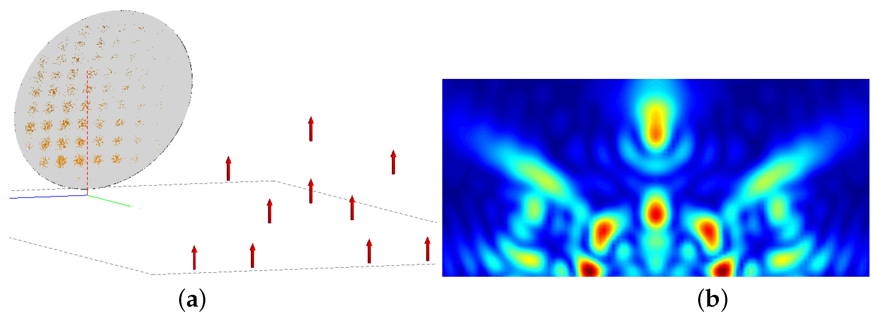
We used FEKO to build a system model and simulated the imaging of ten dipole sources (4 GHz) placed in a circle shape on the object plane. The model structure and the degraded pictures are shown in Figure 7.
As shown in Figure 8, the row above is the step result of the log-polar transformation algorithm. It can be seen that the log-polar transformation basically eliminates the spatial variation characteristics of the blur, and the number and position of the electromagnetic radiation source are consistent with the real conditions. The row below is the result of applying other algorithms to Figure 8a. It can be seen that due to the large blur and the obvious spatial variation characteristics, the direct super-resolution (SR) algorithm and segmentation SR algorithm cannot satisfy the space-invariant hypothesis which results in some speckle noise and false signals. In addition, the only polar transformation method can recover part of the blur, leaving the noise caused by the radial variant blur.
4.3. Deblur of Experiment Results
We built an imaging system in a microwave darkroom and performed imaging experiments on three horizontally-placed, double-ridged horn antennas (3–6 GHz, 10 dBm), as shown in Figure 9. The results are shown in Figure 10.
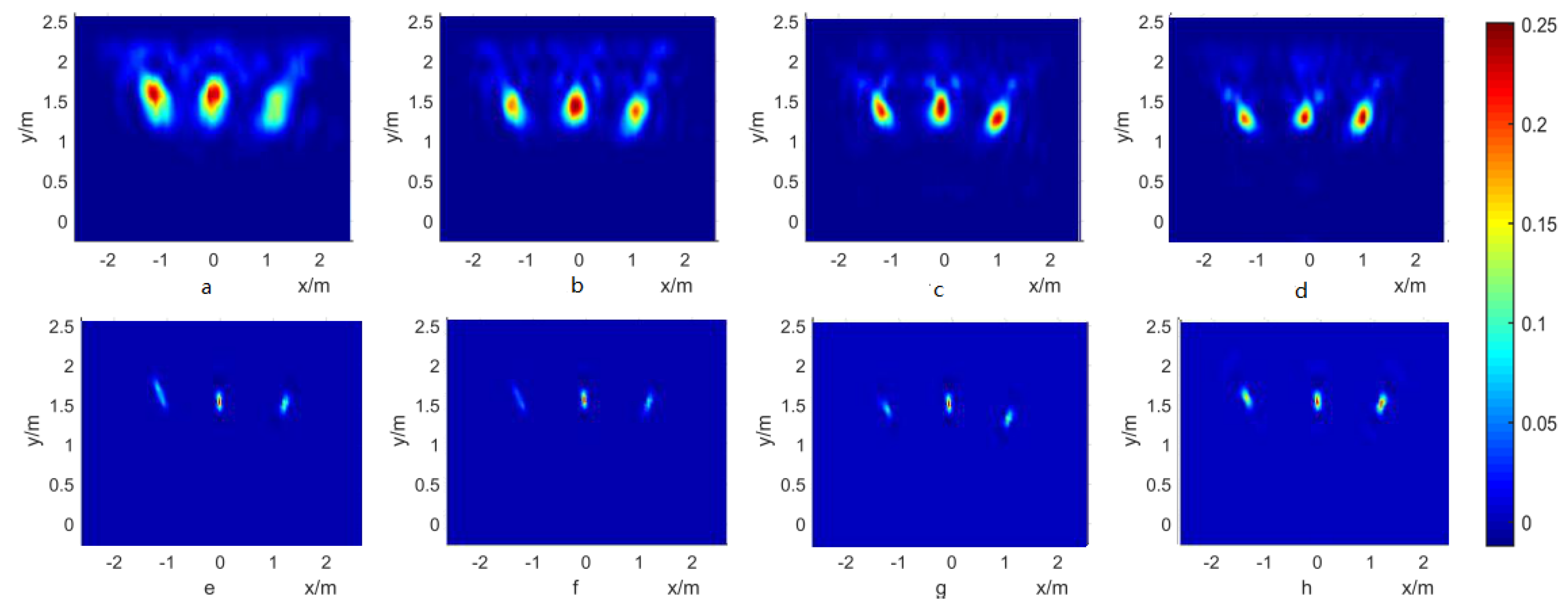
The row above in Figure 10 is the step result of the log-polar transformation algorithm, and the row below shows the results of the other algorithms. It can be seen that the direct SR and segmentation SR algorithms still generate noise and interfere, which will cause mistakes in the judgment and localization of the electromagnetic leakage. The log-polar algorithm can effectively suppress this problem. Figure 11 below shows the results of the imaging (upper) and resolution recovery (lower) results of radiation sources of different frequencies. So, as we can see, the algorithm can be applied to a wide-range spectrum if we can get the PSF.
In theory, the recovered image should have the same resolution and position as the target signal. The resolution can be measured by the beamwidth of the recovered signal. So, we evaluated the results in Figure 11 by the consistency of position and beamwidth of the three signals.
In the evaluation, the positions of different antennae were determined by the x and y-axes (unit: pixel) of the maximum value of their beams. The beamwidth used in this evaluation was introduced from the antenna area and was set at a beamwidth of −6 dB, which means the area (unit: pixel) of the value that is 6 dB less than the peak of the beam. In this paper, it was calculated by the following:
- Step 1 Convert the z-axis of the image matrix into a dB area by log operation.
- Step 2 Mark the pixel as 1 if its value is larger than the peak subtracted by 6 dB and 0 if not.
- Step 3 Calculate the number of 1 in the whole image as the −6 dB beamwidth.
The results are as follows. In Table 1 and Table 2, left means the left signal on the recovered image, and similarly with the center and right. The units of both tables are pixels. Table 1 shows that the positions of the three signals were almost the same and met up with the real antenna. Table 2 shows that the recovery signals had good consistency in beamwidth with each other at different frequencies. The position and beamwidth prove that the method is suitable for wide-frequencies.
The transformation is not complex and the size of image is also not too big, so the time that the algorithm consumes (on the laptop with MatLAB R2014b, Windows 7, Intel I5) is within 1 s. The number of iterations in the L-R iteration method is set to 300 for regularization.
5. Conclusions
In the deblurring processing of focal-plane image, the space-variant characteristic is hard to eliminatedue to its large dimensions. This problem is particularly acute in our focal-plane microwave imaging systems due to the low frequency and off-axis aberration. In this paper, we analyzed the physics model of the space-variant blur and proposed an LPCT method as the preprocessing method before Lucy–Richardson restoration. This algorithm starts from the principle of image blur instead of approximating it, and proved to be effective for the space-variant deblurring of focal-plane microwave imaging. It improves the resolution and accuracy of electromagnetic imaging and detecting in EMC detection significantly. However, this method brings a blind spot, as discussed above, and there is no better solution but to avoid it. In addition, in future work, the interpolation of transformation will be studied further to depress the uneven rise of values and regularization with the L-R algorithm to help to improve the noise problem.
Author Contributions
Conceptualization, S.L. and S.X.; Data curation, M.Y.; Formal analysis, S.L.; Funding acquisition, S.X.; Investigation, S.L. and T.W.; Methodology, S.L., X.H. and Y.L.; Project administration, S.X.; Resources, X.H.; Software, M.Y.; Supervision, S.X.
Funding
This research was funded by Defense Industrial Technology Development Program (Grant No. JCKY2016601B005).
References
- Angel, E.S.; Jain, A.K. Restoration of images degraded by spatially varying pointspread functions by a conjugate gradient method. Appl. Opt. 1978, 17, 2186. [Google Scholar] [CrossRef] [PubMed]
- Woods, J.; Radewan, C. Kalman Filtering in Two Dimensions; IEEE Press: Piscataway, NJ, USA, 1977. [Google Scholar]
- Woods, J. Correction to Kalman Filtering in Two Dimensions. IEEE Trans. Inf. Theory 2003, 25, 628–629. [Google Scholar] [CrossRef]
- Ozkan, M.K.; Tekalp, A.M.; Sezan, M.I. POCS-based restoration of space-varying blurred images. IEEE Trans. Image Process. 1994, 3, 450–454. [Google Scholar] [CrossRef] [PubMed]
- Fish, D.A.; Grochmalicki, J.; Pike, E.R. Scanning singular-value-decomposition method for restoration of images with space-variant blur. J. Opt. Soc. Am. A 1996, 13, 464–469. [Google Scholar] [CrossRef]
- Nagy, J.G.; O’Leary, D.P. Fast iterative image restoration with a spatially varying PSF. In Proceedings of the Optical Science, Engineering and Instrumentation, San Diego, CA, USA, 27 July–1 August 1997; pp. 388–399. [Google Scholar]
- Mikhael, W.B. Restoration of digital images with known space-variant blurs from conventional optical systems. Int. Soc. Opt. Eng. 1999, 3716, 71–79. [Google Scholar]
- Trussell, H.; Hunt, B. Sectioned methods for image restoration. IEEE Trans. Acoust. Speech Signal Process. 1978, 26, 157–164. [Google Scholar] [CrossRef]
- Trussell, H.; Hunt, B. Image restoration of space-variant blurs by sectioned methods. IEEE Trans. Acoust. Speech Signal Process. 1978, 26, 608–609. [Google Scholar] [CrossRef]
- Costello, T.P.; Mikhael, W.B. Efficient restoration of space-variant blurs from physical optics by sectioning with modified Wiener filtering. Digit. Signal Process. 2003, 13, 1–22. [Google Scholar] [CrossRef]
- Guo, Y.P.; Lee, H.P.; Teo, C.L. Blind restoration of images degraded by space-variant blurs using iterative algorithms for both blur identification and image restoration. Image Vis. Comput. 1997, 15, 399–410. [Google Scholar] [CrossRef]
- Du, X.; Xie, S.; Hao, X.; Wang, C. An electromagnetic interference source imaging algorithm of Multi-resolution partitions. High Power Laser Part. Beams 2015, 27, 10. [Google Scholar]
- Sawchuk, A.A.; Peyrovian, M.J. Restoration of astigmatism and curvature of field. J. Opt. Soc. Am. 1975, 65, 712–715. [Google Scholar] [CrossRef]
- Camera, A.L.; Schreiber, L.; Diolaiti, E.; Boccacci, P.; Bertero, M.; Bellazzini, M.; Ciliegi, P. A method for space-variant deblurring with application to adaptive optics imaging in astronomy. Astron. Astrophys. 2015, 579, A1. [Google Scholar] [CrossRef]
- Mourya, R.; Ferrari, A.; Flamary, R.; Bianchi, P.; Richard, C. Distributed approach for deblurring large images with shift-variant blur. In Proceedings of the European Signal Processing Conference, Kos island, Greece, 28 August–2 September 2017; pp. 2463–2470. [Google Scholar]
- Zhang, X.; Wang, R.; Jiang, X.; Wang, W.; Gao, W. Spatially variant defocus blur map estimation and deblurring from a single image. J. Vis. Commun. Image Represent. 2016, 35, 257–264. [Google Scholar] [CrossRef] [Green Version]
- Schuler, C.J.; Hirsch, M.; Harmeling, S.; Scholkopf, B. Learning to Deblur. IEEE Trans. Pattern Anal. Mach. Intell. 2016, 38, 1439–1451. [Google Scholar] [CrossRef] [PubMed]
- Sun, J.; Cao, W.; Xu, Z.; Ponce, J. Learning a convolutional neural network for non-uniform motion blur removal. In Proceedings of the IEEE Conference on Computer Vision and Pattern Recognition, Boston, MA, USA, 7–12 June 2015; pp. 769–777. [Google Scholar]
- Li, L.; Yang, J.; Wang, J.; Deng, Y. An focal plane array space variant model for PMMW imaging. In Proceedings of the IET International Radar Conference, Guilin, China, 20–22 April 2009; pp. 1–4. [Google Scholar]
- Lee, C.; Xiong, B.; Compiled, T. A Course of Optical Information; Dou, J., Ed.; Publishing House: Beijing, China, 2011; pp. 40–41. [Google Scholar]
- Guoguang, E. Light Field Transformation by Paraboloidal Mirror. Acta Opt. Sin. 1995, 15, 593–599. [Google Scholar]
- Arguijo, P.; Scholl, M.S. Exact ray-trace beam for an off-axis paraboloid surface. Appl. Opt. 2003, 42, 3284–3289. [Google Scholar] [CrossRef] [PubMed]
- Arguijo, P.; Scholl, M.S.; Paez, G. Diffraction patterns formed by an off-axis paraboloid surface. Appl. Opt. 2001, 40, 2909–2916. [Google Scholar] [CrossRef] [PubMed]
- Sawchuk, A.A. Space-variant image restoration by coordinate transformations. J. Opt. Soc. Am. 1974, 64, 138–144. [Google Scholar] [CrossRef]
- Wolberg, G.; Zokai, S. Robust image registration using log-polar transform. In Proceedings of the International Conference on Image Processing, Florence, Italy, 13–19 September 2000; Volume 1, pp. 493–496. [Google Scholar]
- Wang, L.; Li, Y.J.; Zhang, K. Application of target recognition algorithm based on log-polar transformation for imaging guidance. J. Astronaut. 2005, 26, 330–333. [Google Scholar]
- Lucy, L.B. An iterative technique for the rectification of observed distributions. J. Astron. 1974, 79, 745. [Google Scholar] [CrossRef]
- White, R.L. Image restoration using the damped Richardson-Lucy method. In Proceedings of the Instrumentation in Astronomy VIII, International Society for Optics and Photonics, Kona, HI, USA, 21–24 September 1994. [Google Scholar]
- Lu, J.K.; Zhong, S.G.; Liu, S.Q. Analytic Extension. In Introduction to the Theory of Complex Functions; World Scientific Publishing Company: Singapore, 2002; pp. 178–199. [Google Scholar]
Figure 1.
Schematic diagram of an off-axis parabolic (OAP) imaging system.

Figure 2.
Off-axis parabolic and its focal plane.
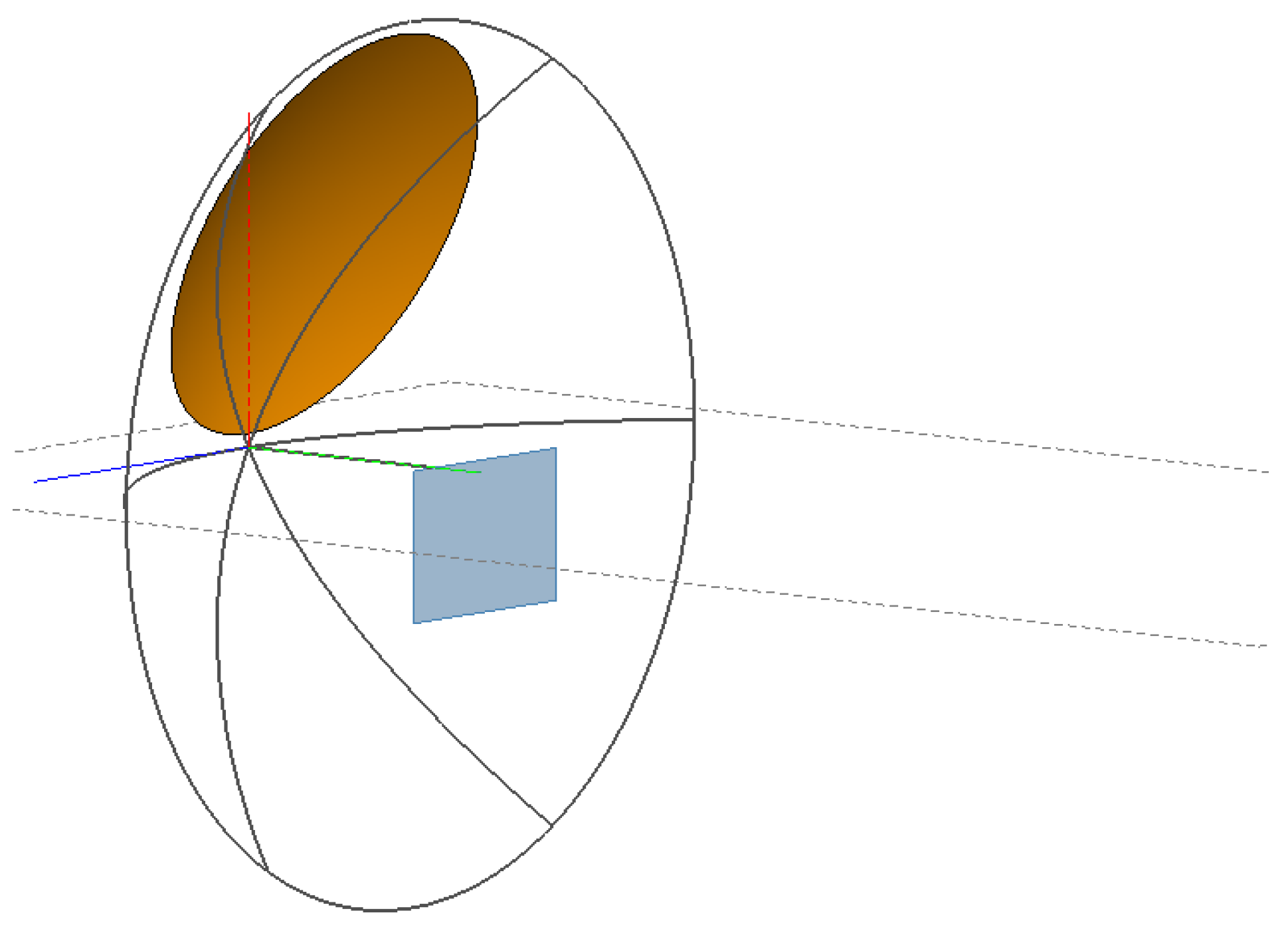
Figure 3.
(a): y-z plane of the blur image with three points located at (x, y) = (0, 0.5 m), (0, 1 m), and (0, 2 m); (b): the result of log-polar transformation of the left one.The unit of x-axis is pixel.
Figure 3.
(a): y-z plane of the blur image with three points located at (x, y) = (0, 0.5 m), (0, 1 m), and (0, 2 m); (b): the result of log-polar transformation of the left one.The unit of x-axis is pixel.
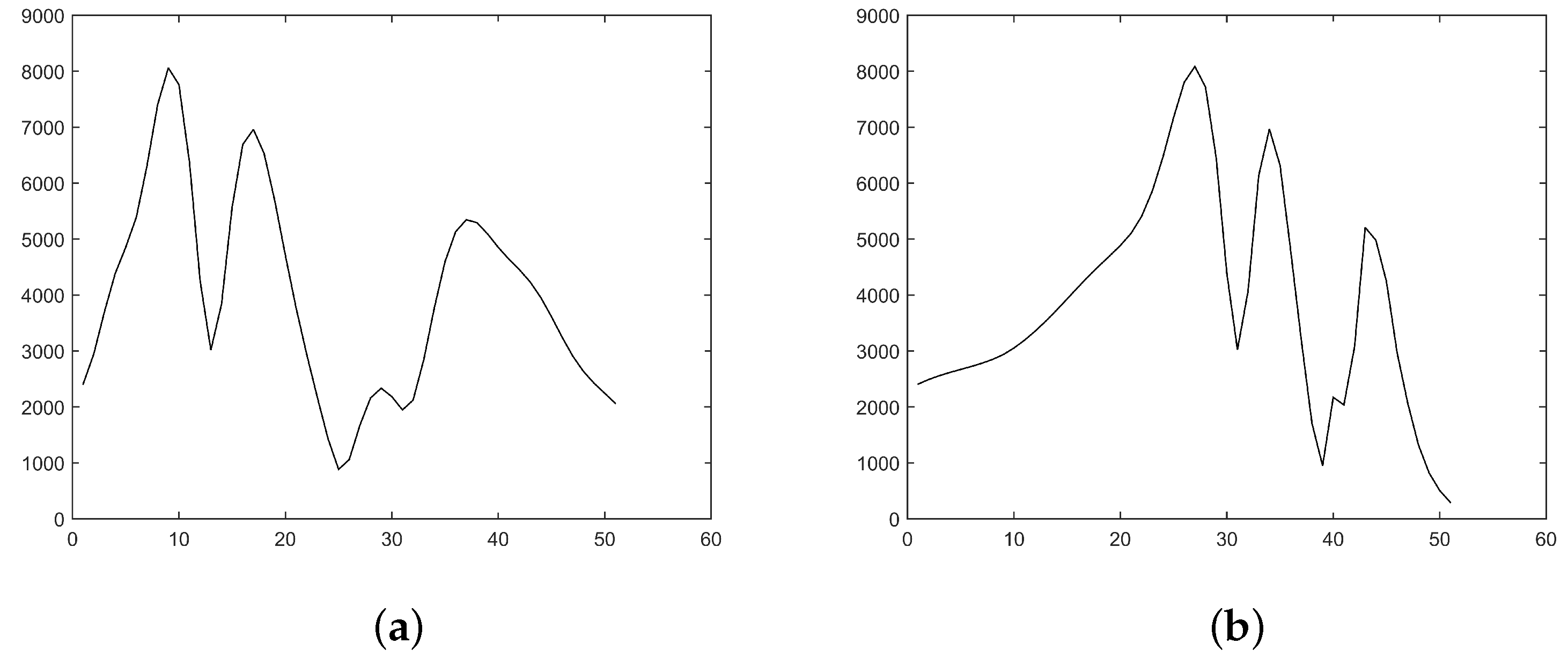
Figure 4.
The diagram of the log-polar transformation: before (a) and after(b).
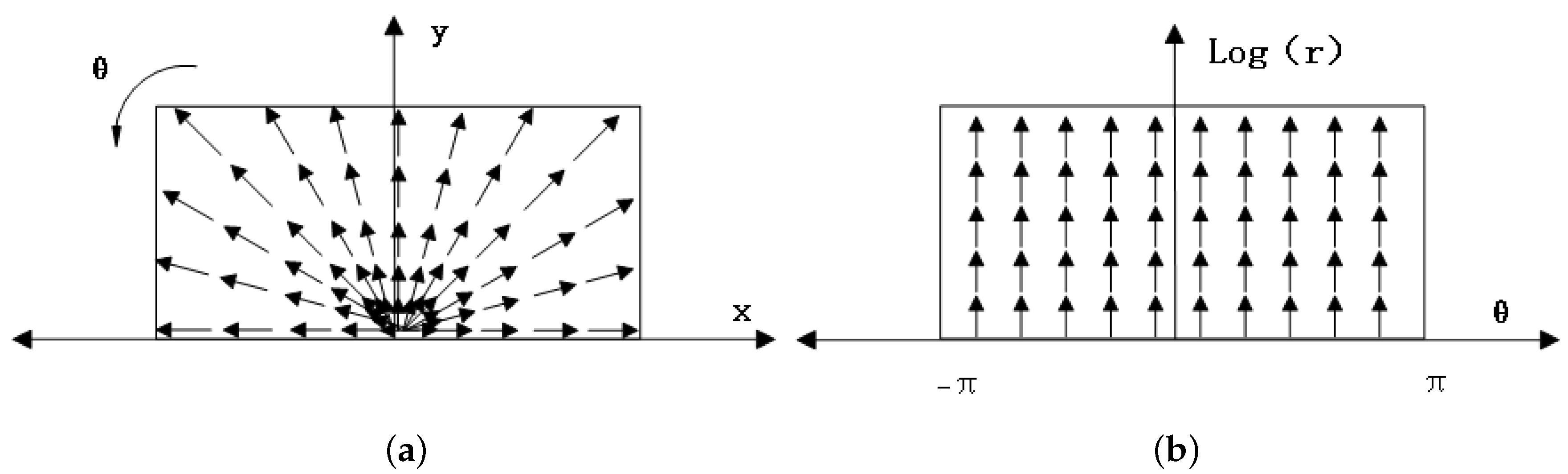
Figure 5.
Flow chart of log-polar transformation and L-R algorithm super resolution.
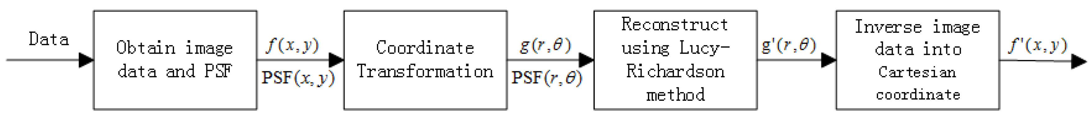
Figure 6.
The 3 GHz PSFs of different methods: (a) the PSF of direct deconvolution algorithm; (b) the polar transformation’s PSF; (c) the PSF of our method; and (d) the PSF of the segmentation method.
Figure 6.
The 3 GHz PSFs of different methods: (a) the PSF of direct deconvolution algorithm; (b) the polar transformation’s PSF; (c) the PSF of our method; and (d) the PSF of the segmentation method.
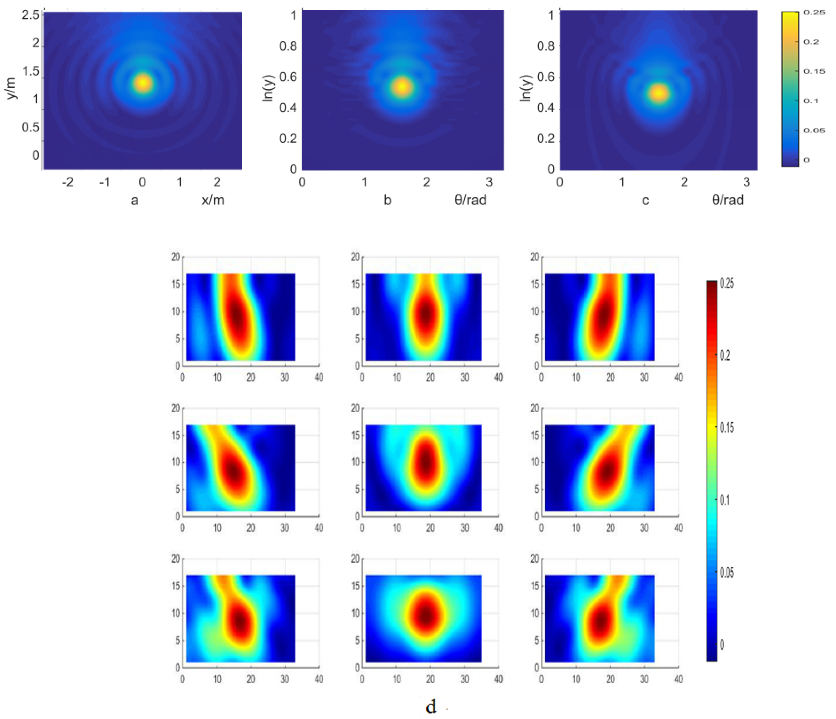
Figure 7.
(a) Simulation of 10 dipole sources (4 GHz,1 V/m); (b) resulting image.

Figure 8.
Row above: (a) Blur image; (b) after log-polar transformation; (c) results of the L-R method; (d) final result; row below, from left to right: results of (e) the direct L-R method; (f) polar transformation with the L-R method; (g) log-polar transformation with the L-R method (the same as (d)); (h) segmentation with the L-R method.

Figure 9.
The off-axis parabolic reflector antenna with optical-electronic sensors (a) and horn antennas on the object plane (b).
Figure 9.
The off-axis parabolic reflector antenna with optical-electronic sensors (a) and horn antennas on the object plane (b).

Figure 10.
(a) blur image; (b) after log-polar transformation; (c) result of L-R method; (d) final result; (e) result of direct L-R method; (f) polar transformation with L-R method; (g) log-polar transformation with L-R method; (h) segmentation with L-R method.
Figure 10.
(a) blur image; (b) after log-polar transformation; (c) result of L-R method; (d) final result; (e) result of direct L-R method; (f) polar transformation with L-R method; (g) log-polar transformation with L-R method; (h) segmentation with L-R method.
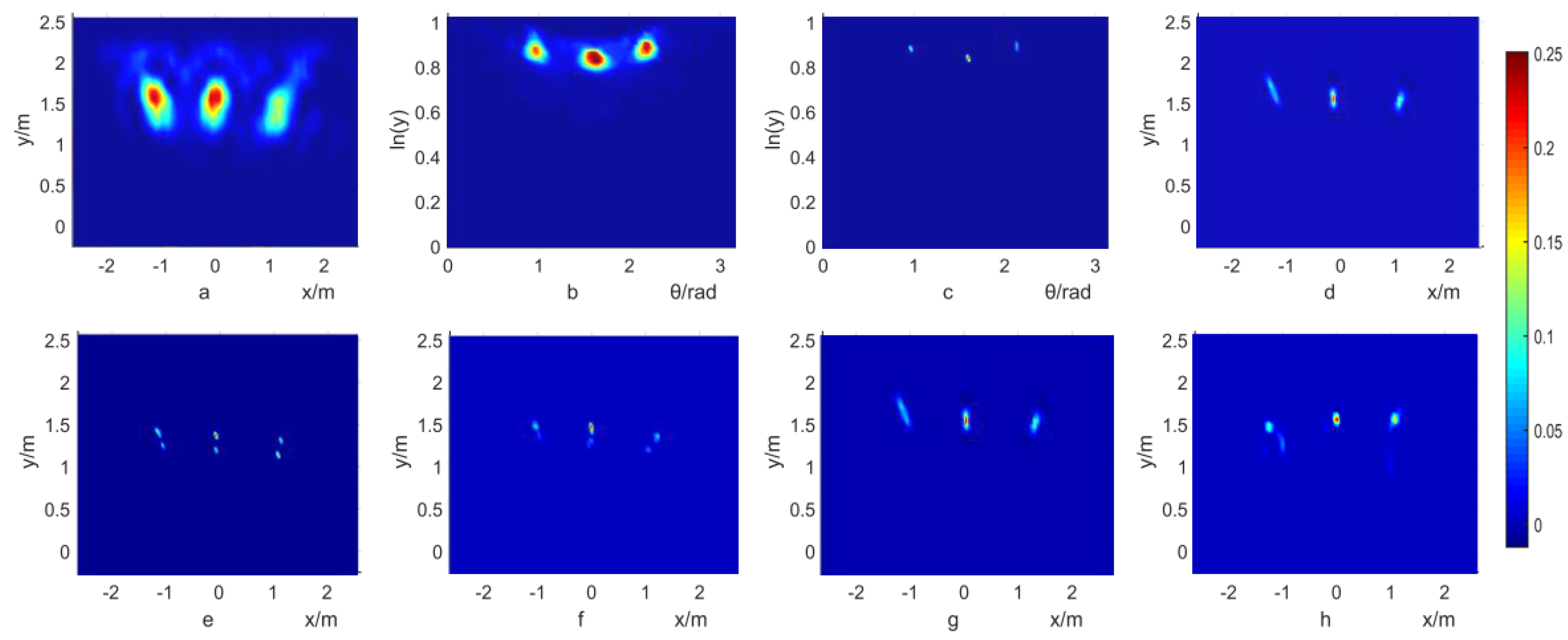
Figure 11.
Blur image of the radiation antenna at frequencies of (a) 3 GHz; (b) 4 GHz; (c) 5 GHz; (d) 6 GHz; restoration result by log-polar transformation at (e) 3 GHz; (f) 4 GHz; (g) 5 GHz; and (h) 6 GHz frequency.
Figure 11.
Blur image of the radiation antenna at frequencies of (a) 3 GHz; (b) 4 GHz; (c) 5 GHz; (d) 6 GHz; restoration result by log-polar transformation at (e) 3 GHz; (f) 4 GHz; (g) 5 GHz; and (h) 6 GHz frequency.

Table 1.
The positions of recovered signals at all frequencies.
| 3 GHz | 4 GHz | 5 GHz | 6 GHz | |
|---|---|---|---|---|
| Left | (36,28) | (32,28) | (32,28) | (34,25) |
| Center | (33,50) | (33,50) | (33,50) | (33,50) |
| Right | (33,73) | (33,73) | (30,71) | (33,73) |
Table 2.
The beamwidth of recovered signals at all frequencies.
| 3 GHz | 4 GHz | 5 GHz | 6 GHz | |
|---|---|---|---|---|
| Left | 2 | 2 | 2 | 3 |
| Center | 6 | 6 | 6 | 6 |
| Right | 7 | 7 | 8 | 10 |
© 2018 by the authors. Licensee MDPI, Basel, Switzerland. This article is an open access article distributed under the terms and conditions of the Creative Commons Attribution (CC BY) license (http://creativecommons.org/licenses/by/4.0/).
Share and Cite
MDPI and ACS Style
Luan, S.; Xie, S.; Wang, T.; Hao, X.; Yang, M.; Li, Y. A Space-Variant Deblur Method for Focal-Plane Microwave Imaging. Appl. Sci. 2018, 8, 2166. https://doi.org/10.3390/app8112166
AMA Style
Luan S, Xie S, Wang T, Hao X, Yang M, Li Y. A Space-Variant Deblur Method for Focal-Plane Microwave Imaging. Applied Sciences. 2018; 8(11):2166. https://doi.org/10.3390/app8112166
Chicago/Turabian StyleLuan, Shenshen, Shuguo Xie, Tianheng Wang, Xuchun Hao, Meiling Yang, and Yuanyuan Li. 2018. "A Space-Variant Deblur Method for Focal-Plane Microwave Imaging" Applied Sciences 8, no. 11: 2166. https://doi.org/10.3390/app8112166
Note that from the first issue of 2016, this journal uses article numbers instead of page numbers. See further details here.