An Optimal Energy Management Method for the Multi-Energy System with Various Multi-Energy Applications

1
School of Electrical and Electronic Engineering, North China Electric Power University, Beijing 102206, China
2
China Electric Power Research Institute, State Grid Corporation of China, Beijing 100192, China
3
State Grid Jiangxi Economic Research Institute, Jiangxi Electric Power Corporation, Nanchang 330043, China
*
Author to whom correspondence should be addressed.
Appl. Sci. 2018, 8(11), 2273; https://doi.org/10.3390/app8112273
Submission received: 5 October 2018
/
Revised: 26 October 2018
/
Accepted: 2 November 2018
/
Published: 16 November 2018
(This article belongs to the Special Issue Smart Home and Energy Management Systems 2019)
Abstract
:As the development of the multi-energy system (MES), various ME applications are deployed. ME applications not only bring advanced functionalities to the MES, but also show great potentials in promoting the operation performance of the MES, especially improving the accommodation of renewable energy sources (RES). However, the realization of these potentials largely relies on the energy management, which shall facilitate the effective function of each ME application and the coordinated collaboration of all the ME applications. Without a comprehensive energy management methodology, ME applications may mutually interfere, which not only hinder the RES utilization, but also may harm the MES operation performance. In this premise, this paper integrates the energy management model of the combined cooling, heat and power plants, power-to-hydrogen/gas-to-power plants, and demand side management model of the EV charging loads into the energy management model of the MES, and proposes an comprehensive optimal day-ahead energy management framework to simultaneously improve the profit, RES utilization rate, and energy saving performance of the MES. To address the proposed optimization model, Elitist Non-dominated Sorting Genetic algorithm II algorithm is employed to heuristically find the Pareto-optimal results. Finally, case studies prove the effectiveness of the proposed methodology.
Keywords:
energy management; multi-energy application; CCHP; P2H/G2P; EV; demand side management; optimization1. Introduction
Driven by the global warming and fossil fuel depletion, recent years have witnessed the development of the multi-energy system (MES) and the proliferation of the renewable energy sources (RES) [1,2,3,4,5]. RES brings significant energy, environment, and economic benefits. However, due to its intermittency and unpredictability nature, the supply curve of the RES usually fails to match the load profile, which may stress the supply-load balance and threaten the operation of the multi-energy system (MES) [4,5]. Due to this, power system experiences huge amounts of RES curtailment, which causes lots of waste. In the future, the RES penetration will be even higher, thus calling for further intensified and more flexible accommodation mechanisms. Fortunately, with the development of the MES, more and more new cross energy sector ME applications come into being, such as multi-generation application, such as combined cooling, heat, and power (CCHP) plant, power-to-Hydrogen and gas-to-power (P2H/G2P) plant, and electric vehicle (EV), which not only bring advanced new functionalities to the MES, but demonstrate promising potentials in dealing with the poor utilization problem of the RES at the same time [6,7,8,9,10,11,12,13,14].
CCHP and P2H/G2P are multi-energy generating technologies. As a CCHP plant is supposed to provide cooling, heat, and electricity supply at the same time, it is usually composed of multiple types of energy generating devices, which provide abundant generating options and redundant energy pathways [7,13,14]. For instance, heat can be produced by electrical heaters with electricity, or by combustion heat generators with fuel; cooling can be produced by an electric chiller with electricity, or by heat pumps with heat. It suggests that the input and output of CCHP plant can be adjusted with purposes while meeting the ME demands. Reference [6] investigates the impact of the flexible dispatch if the CCHP plants on the operation performance of the integrated electrical and natural gas network, reference [7] investigates its potential in providing real time demand response services. It is this flexibility both regards generation and system dispatch that could be particularly relevant to providing real time ancillary and accommodating the RES. As for P2H/G2P facilities, they can store power into hydrogen through P2H process, or reversely release the power through G2P process [15]. Its use in accommodating RES is quite intuitive and has been widely studied [9,15,16,17]. Reference [15] assesses the potential for P2H to increase wind power dispatchability, and reference [17] explores how to integrate P2H into power systems for load balancing. In [10,18], the potential of the energy hub equipped with a P2H facility (electrolyzer) and a gas-to-power (G2P) facility (hydrogen gas turbine) is illustrated in accommodating the volatility introduced by a large wind power penetration. With CCHP plants and P2H/G2P plants deployed, the excess of RES outputs can be stored in hydrogen, or/and fuel the electricity-driven devices to supply the ME demands; and when there is a lack of RES outputs, the electricity stored in hydrogen can be released through G2P process, and ME demands could mainly be produced by the fuel-dependent devices.
As a greener means of transportation, EVs have gained increasingly higher market share in recent years, especially in China [19]. It poses a challenge as well as a significant opportunity to the conventional energy system [20,21]. Though the EV charging loads risk aggregating the daily peak loads and causing power congestions, appropriate demand side management could encourage the EV customer to delay their charging behavior, which can shift the charging loads from peak hours to off-peak hours [22,23,24,25]. In the same way, through scheduling EV charging loads to coincide with periods of strong wind or sun, greater adoption of RES could be achieved. Many studies about the demand side management of EV charging loads have been published [24,25], and economic signal are mostly employed to pre-schedule the EV charging customers’ load profile. Reference [23] proposes a decentralized demand side management method based on time-varying prices, to both maximize the aggregators’ profits while minimize the consumers’ costs. Reference [24] jointly considers the customers’ charging requirements and system load profile, proposes a coordinated charging strategy aiming to achieve peak shaving by heuristically setting dynamic time-of-use (TOU) pricing strategy. In [25], the demand response of EV customers to peak-valley pricing is modelled based on price elasticity matrix.
On the one hand, these ME applications bring advanced new functionalities and dispatch resources to the MES and provide possibilities in improving the MES operation, including accommodating more RES. On the other hand, they increase to the total complexity of the operation model of the MES and complicate the entire energy management process. Without a comprehensive energy management model, they may operate in less optimal conditions and add up the cost, or in uncoordinated ways and offset each other, either of which will harm the operation performance of the MES and waste these valuable assets of the MES. Meanwhile, rare cross-sectional researches that include them all are conducted.
On these premises, based on the economic dispatch model of the power system, this paper proposes a novel day-ahead optimal energy management method for the MES with CCHP, P2G, and EV, to simultaneously promote the RES utilization, and the economic and energy-saving performance of the MES. At first, the operation of the CCHP plant, P2G plant, and the demand response model of the EV charging load under TOU schemes are modelled respectively. Among them, the modelling of the CCHP devices are based on the concept of “Energy Hub”, and the demand response of EV charging load is based on the price elasticity matrix. Then, the model of these three ME applications are integrated in the holistic dispatch model of the MES. Based on the developed model, three objectives are formulated to simultaneously promote the RES utilization rate, and the economic and energy saving performance of the MES. Considering the proposed optimization model is mathematically a multi-objective, mixed integer non-linear model, which cannot be easily solved with classical mathematical techniques, the Elitist Non-dominated Sorting Genetic Algorithm II (NSGA-II) [26] is applied to find Pareto optimal results. The main contributions of this paper are threefold:
- The energy management of CCHP plant and P2H/G2P plant, and the demand side management of EV charging loads are modelled, and integrated in the energy management model of the MES as dispatch resources.
- Base on the developed model, a multi-objective optimal energy management problem is proposed to facilitate the cooperation of the ME applications, and simultaneously promote the RES utilization, and the overall economic and energy-saving performance of the MES.
The rest of this paper is organized as follows: Section 2 presents the operation models of the CCHP plants, P2H/G2P plants, and the demand response model of the EV charging loads. Based on the developed models, a multi-objective optimization model for the MES energy management is proposed in Section 3, and tested on cases studies in Section 4. At last, the paper is concluded in Section 5.
2. Mathematical Modelling of ME Applications
2.1. Modelling of CCHP Plant
A CCHP plant is composed of two sides of ME devices: cogeneration side and cooling power production side.
Cogeneration side:
- Combined heat and power units (CHP) are the core of CCHP plants, which generates both heat and electricity. ηW and ηQ are used to describe the ratio of electric power output and heat power output to the fuel thermal energy input respectively.
- Combustion heat generators (CHG) are usually the thermal backup of the CHP. ηt is used to describe the ratio of heat power output to the fuel thermal energy input.
- Cooling power production side:
- Compression electric refrigeration generators (CERG) are widely used for producing cooling power, both for air conditioning and industrial purposes.
- Electrical heat pumps (EP) are a bimodal CCHP device which can produce heat and cooling power with electric power input.
- Water adsorption refrigeration generators (WARG) are heat-driven cooling power producers.
- Gas absorption refrigerator generators (GARC) are fuelled by natural gas, but are less widespread [27].
Figure 1 shows the inputs and outputs of the ME devices above with their respective performance indicator. F represents the fuel thermal energy, W represents electricity, Q represents heat, and R represents cooling power. Coefficient of performance (COP) is defined as the ratio of cooling power output to the energy input, which is used to represent the performance indicator of cooling production devices.
To integrate the operation model of a CCHP plant into the dispatch model of the MES, the model of each component CCHP device should be developed first. For a component CCHP device, and are used to denote its input and output array respectively, the mapping between energy input and output is described with the efficiency matrix H as in (1). Each element in H relates one particular input to a certain output with relevant energy conversion efficiency η, whose two subscript respectively denote the type of energy output and the type of energy input.
Take the illustrative scheme of a CCHP plant in Figure 2 as an example. It is composed of four CCHP devices, among which are energy pathways: the yellow line represents electric power flow; the green line represents fuel energy flow; the red line represents heat power flow; and the blue line represents cooling power flow. It receives electricity supply Wi from the Electrical Distribution System (EDS) and fuel Fi from the Fuel Distribution System (FDS). Electricity can be both bought from and sold to markets through the EDS. Heat demands can be met by exploiting CHP, CHG, and the EP (heating mode). The cooling demand can be met by using the WARG or/and the EP (cooling mode). Electricity can be drawn from the EDS and/or produced by the CHP (and can be sold back as well). Considering there is no heat storage, extra heat QDump will be dumped. It is the abundant production options and redundant energy pathways that provide possibility for CCHP plant to be part of serving the RES accommodation, and promoting the MES operation.
In order to model its internal energy flows, energy dispatch factor (EDF) is introduced, which is defined as an array of elements that mark the relative energy dispatch at flow splitting points (bifurcations) within the CCHP plant [6,12]. For the CCHP plant in Figure 2, the EDF is defined as . denotes the proportion of electricity that is used for the heat production in all the electricity supply of the EP. Then, the input and output relation of the CCHP plant can be described with (2) and (3), where denotes local ME demands, and denotes the energy exchange with energy distribution networks:
With (2) and (3), the energy management of the CCHP plant can be reflected through a matrix formulism, which makes it easy to be embedded within the optimization model of the MES.
2.2. Modelling of P2H/G2P Facility
The schematic of a typical P2H/G2P facility is given in Figure 3. In Figure 3, the area surrounded by dotted line represents P2H/G2P plant, which is composed of P2H (electrolyzer) unit, G2P (hydrogen turbine) unit and hydrogen storage serving as a buffer.
Figure 4 gives the diagram of how RES output variation is accommodated with P2H/G2P plants. When there is a surplus of RES generation, P2G is employed to store them into hydrogen by electrolysis in high-pressure hydrogen tanks or caverns. During periods of low RES generation or high power demand, the stored energy can be converted to power through the G2P process. Therefore, three operation modes are considered in the modelling process: P2H mode, G2P mode, and idling mode. In P2H mode, the plant acts as an electric demand, while in G2P mode an electrical generator. In the idling mode, the facility is on standby for either P2H or G2P. In (4), I(t) is used to indicate the operation mode of the concerned P2H/G2P plant.
Then, the output of the P2H/G2P plant PHdr(t) is defined by the linear relationship between the power that charges the hydrogen storage in P2H mode and the power that discharges it in G2P mode, as in (5) and (6). In (5), ηG2P, ηP2H are the conversion efficiencies of G2P and P2H processes respectively, , and , are the lower and upper output limits of the corresponding operation modes.
The hydrogen storage level Hsto(t) is constrained by (7)–(9), where (8) ensures that the storage level is sufficient to provide service, and (9) is to avoid end-of-horizon effects by setting the final hydrogen storage level to be close to its initial value.
and are the lower and upper storage limits; Δt represents the given time interval; ΔHsto is a pre-specified small value; Hoth represents the hydrogen product directly demanded by other energy sectors, which is constrained by (10). In (10) represents the upper limits of the Hoth.
2.3. Demand Response of EV
In economics, the price-elasticity of demand presents the relative variation of demand caused by the relative variation of the product price, which is the ratio of rate of demand increment over the rate of price increment [28]. The consumer’s response to TOU pricing scheme belongs multi-period response, which means the electricity consumptions of most consumers in a period is not only related to the electricity price in the current period, but also related to the electricity prices in adjacent periods [25,28,29]. Therefore, the mathematical expression of electricity consumption in a certain period and the price in each period can be expressed as in (11):
In (11), one day is divided into N periods, Dev,i is the electricity consumption in period i, and ρi is the electricity price in period i. N periods are categorized into three kinds: peak, flat, and valley. Around the given equilibrium points in each period, Equation (11) can be linearized with the first order Taylor expansion:
Define the self-elasticity coefficient εii and cross-elasticity coefficient εij as in (13):
So the price-elasticity matrix of demand can be derived as in (14):
where ΔDev,i denotes the electricity consumption increment during period i, and Δρi the price increment during period j.
According to (12), the linearized relations between electricity consumption and price around respective equilibrium points in peak, flat and, valley periods can be described with (15)–(17), where Dev,h, Dev,f, and Dev,v are the electricity consumption during peak period, flat period, and valley period respectively; ρh, ρf, and ρv are the electricity price during peak period, flat period, and valley period respectively. kh and bh, kf and bf, and kv and bv define the linearized relations around the equilibrium points between the electricity consumption and price during each period. ΩH, ΩF, and ΩV denote the peak, flat, and valley periods sets respectively.
With (15), the self-elasticity defined in (13) can be rewritten into (16).
Assume the total daily electricity consumption remains the same with or without TOU pricing scheme, then (17) can be obtained.
Take the partial derivatives concerning Dev,j for both sides of the (17), we can get:
With (18), the cross-elasticity coefficient εij can be obtained as in (19):
With (14), (16), and (19), the daily electricity consumption under the TOU pricing scheme can be obtained as in (20), Where ρTOU and ρ0 denote the TOU price and the base price.
3. Energy Management Framework
Based on the model of the three ME applications that are developed in Section 2, a novel optimal energy management framework for the ME system with ME applications is proposed, and its mathematical model is given in detail in this section. The decision variables vector V is defined as in (21). In (21), PG and PHdr are the output arrays for generators and P2H (G2P) plants respectively, p is the daily charging price array of EVs, and α is the EDF vector for CCHP plants.
The objective function comprises of three individual objectives: F1, F2, and F3. F1 is modeled as the profits of the MES, which is defined as the total revenue through selling electricity minus the generation cost:
In (22), ΩB, ΩChr, ΩG, ΩHdr, and ΩCCHP are the buses set, generators set, EV charging facilities set, P2H/G2P plants set, and CCHP plants set; PG is the output of the generator, PP2H and PG2P are the output of P2H/G2P plant in P2H and G2P process, respectively, and aj, bj, cj, bP2H, cP2H, aG2P, bG2P, and cG2P are their corresponding consumption characteristic factors; I is the state indication of P2H/G2P plant; D is the electric load and PChr is the EV charging load; is the hourly selling price of electricity, is the hourly price for EV charging, and are the fuel price for power production, and heat, cooling power production.
F2 is modelled as in (23) to describe the daily utilization rate of the renewable energy outputs:
In (23), ΩR denotes the RES generating units set, PR and PR_max denote the outputs and maximal outputs of the RES.
F3 is modelled to describe the energy saving performance of the concerned MES [6]. In (24), WCCHP, QCCHP, and RCCHP are the electricity, heat, and cooling output of CCHP plants, ηF is the thermal energy rate of the fuel injection.
The constraints part are composed of electrical network constraints and ME applications constraints.
Equations (25)–(27) are electrical network constraints. Equation (25) represents the active and reactive power balance for each bus. Equation (26) represents the output limits of generators. Equation (27) represents the operational limits on the apparent power and the steady-state voltage magnitude. PGi and QGi denote the active and reactive power outputs, PLi and QLi denote the active and reactive power loads, Ui denotes the voltage magnitude of Bus i and θij denotes the voltage angle gap between Bus i and Bus j, Gij, and Bij denote the real and imaginary parts of the ith row the jth column element in the nodal admittance matrix. Sij denotes the apparent power between bus i and bus j.
Equations (28)–(30) are the CCHP plants constraints. In (28) and (29), and are the maximum input and minimum input of ME device x in the CCHP plant m, and its maximum output and minimum output. In (30), and are the ME input of the CCHP plant m and local ME demands, is the ME exchange between the CCHP plant m and the external energy distribution networks.
The constraints of P2H/H2P plants are defined in Section 2.2 as in (4)–(10).
Equations (31) and (32) are the EV charging constraints. In (31), and are the minimum and maximum price of the EV charging price. In (32), is the maximum EV charging load at the EV charging facility i.
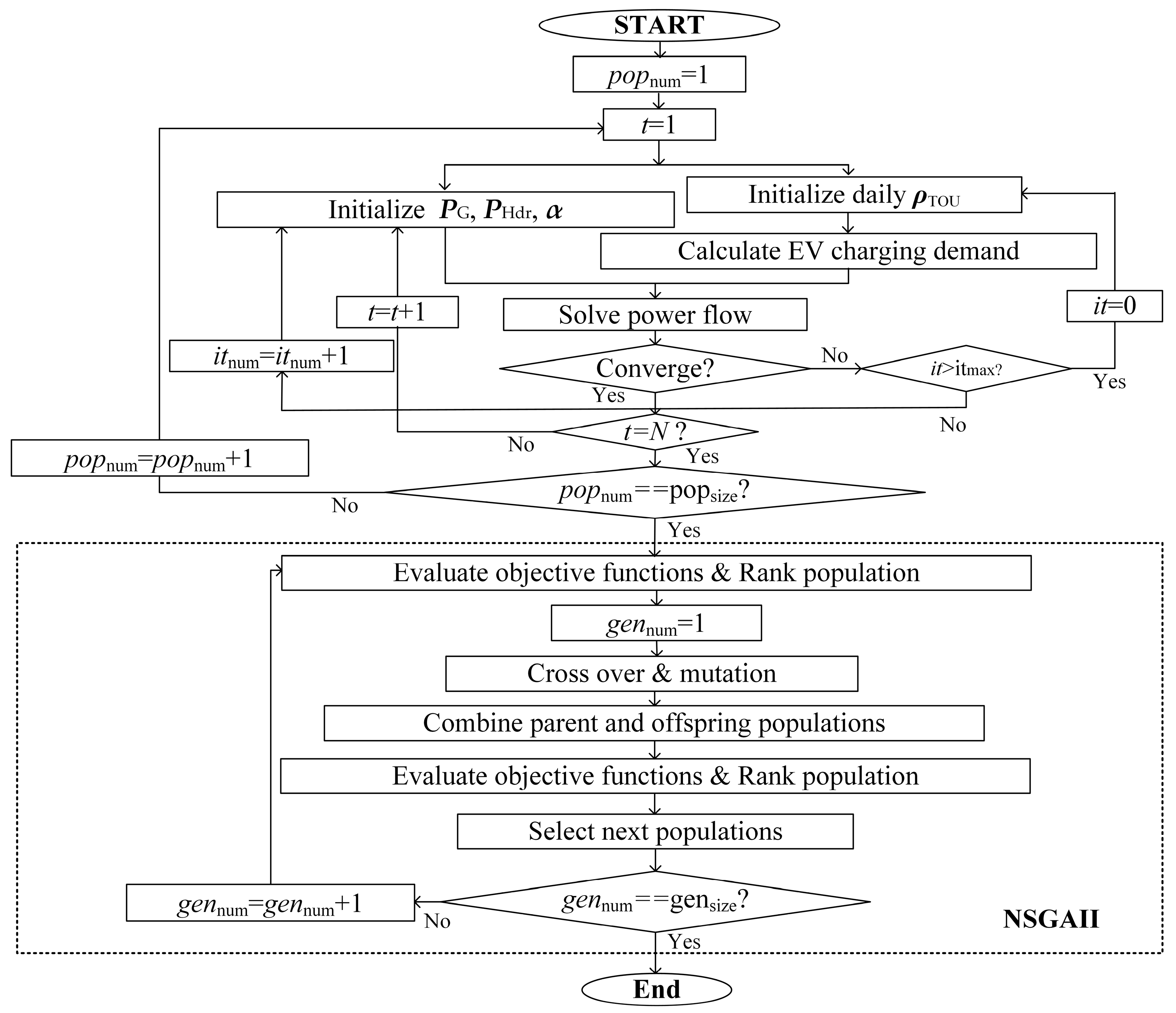
The proposed energy management model is mathematically a multi-objective, mixed integer non-linear optimization model, and NSGAII is employed to address it. The computation process shown in Figure 5 can be summarized as follows.
STEP 1: Initialize the population number popnum, generation number gennum, and starting time t, assuming a day is divided into N periods.
STEP 2: If popnum = popsize, go to Step 5; if not, initialize daily EV charging price ρTOU, and calculate EV charging load under ρTOU.
STEP 3: Initialize outputs of generators PG, outputs of P2H/G2P plants PP2G, and EDF of CCHP plants α.
STEP 4: Solve power flow. If the power flow results converge, go to STEP 5; if not converge, and iteration times it < itmax, reinitialize PG, PP2G and α, it = it + 1, go to STEP 3; Otherwise, reinitialize ρTOU, it = 0, go to STEP 2.
STEP 5: if t < N, t = t + 1, go to STEP 6; else, popnum = popnum + 1, go to STEP 2;
STEP 6: Evaluate and rank each population.
STEP 7: After crossing over and mutation process, offspring population and parent population are evaluated, ranked and then selected.
STEP 8: if gennum = gensize, the remaining results consist of the Pareto-optimal results; if not, gennum = gennum + 1, go to STEP 6.
4. Simulation and Results
Two case studies consisting of a six-bus (Case A) [30] and the modified IEEE 39-bus system (Case B) are performed in this section. Case A is designed to first demonstrate the accommodating effects of the CCHP utilizations, P2H/G2P utilizations, and demand response of EV charging loads respectively, and then demonstrate the performance loss when no energy management strategies are used. Case B is designed to show the effectiveness of the proposed optimal energy management method.
4.1. Case A
The six-bus system shown in Figure 6 is studied over the 24-h of operation. It includes three conventional generators: G1, G2, and G3. A CCHP plant, a P2H/G2P plant, a wind turbine, and an EV charging unit are all located on Bus 4. Parameters of them are listed in Table 1, Table 2 and Table 3. Consider the maximum and minimum capacity of the hydrogen storage are 200 MWh and 40 MWh respectively, and its initial storage level is 80 MWh [12]. Assume the efficiency for P2H and G2P processes are 80% and 40%, respectively. The hourly electric demand, EV charging demand, forecasted wind power (with 200 MW installed capacity), and ME demands over the 24-h horizon are listed in Figure 7. The gas price is 3.71 $/MBtu for the CCHP production, and the selling price of electricity is 51.22 $/MWh (23:00–7:00), 73.27 $/MWh (10:00–17:00 and 21:00–23:00), and 85.04 $/MWh (9:00–10:00 and 18:00–20:00). Consider the separate generation efficiencies are = 0.4, = 0.9, and COPSP = 3.5 [16]. The parameters of the NSGAII algorithm are set as follows: the population size popsize = 100, the evolution time gensize = 1000, and the crossover and mutation probabilities are 0.8 and 0.2, respectively.
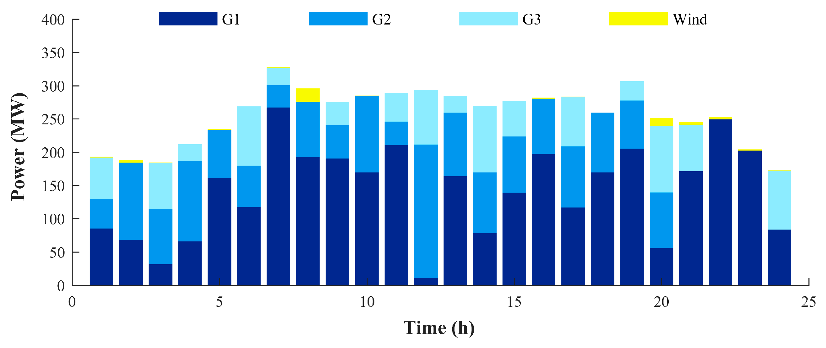
In order to show their respective potentials in accommodating the RES, six cases are designed as in Table 4. For Case A, only RES utilization rate is considered as the objective of the optimization problem. Among the six cases, Case 1 is the control case—a six-bus with a wind turbine. The hourly dispatch results for Case 1–6 are given in Figure 8, Figure 9, Figure 10, Figure 11, Figure 12 and Figure 13 respectively. In Figure 9, Figure 10 and Figure 11, (a) shows the outputs of generators, and (b) shows the dispatch results of each ME application. Compare Figure 8 and Figure 11, it could be easily noticed that the EV charging load under TOU pricing schemes could effectively enlarge the yellow area—improve the wind power utilization.
In Figure 9, when the wind power is abundant, the generation of the ME demands mainly depends on the free wind power. For instance, in Figure 9b, Wi peaks during 8:00–21:00. When the forecasted wind power slumps at 20:00, the production of the CCHP plant turns to rely on the natural gas input, especially when some generators are offline. For instance, at 23:00, only G1 is online, and at 24:00, 1:00, only G1 and G3 are online. In these periods, CCHP plant generates more electricity on purpose to feedback the electric networks.
In Figure 10, the P2H/G2P plant operates in P2H mode at 3:00, 7:00–8:00, 15:00, 17:00, 20:00–21:00 and 23:00. Among them, at 3:00 and 15:00, the wind power is abundant, though the conventional generators’ outputs are relatively low, the total power supply is enough for the electric demand and P2H process; At 7:00, 17:00, the electric demands reach peaks, but the wind power and generator outputs peak as well, extra power are then stored in hydrogen tank for the G2P process in the following hours. The P2H/G2P plant operates in G2P mode at 1:00, 4:00, 9:00, 16:00, 18:00, and 22:00. At 1:00, 4:00, and 22:00, the outputs of generators are relatively low; at 9:00, 16:00, and 18:00, electric load reach peaks, while the generators’ outputs and wind turbine outputs are relatively low. Electricity that are pre-stored in hydrogen tank then released to cope with the power shortage.
In Figure 11, at 5:00, 8:00, and 11:00, the electric demand is high while the power supply is relatively low, thus the increase in price could effectively decrease the EV charging loads in these periods. At 3:00 and 9:00, the power supply is abundant while the electric load is relatively low, thus the decrease in charging price could encourage consumers’ charging behaviors in these periods, which not only saves them more money, but also alleviate the power congestion. So are at 7:00, 12:00, and 15:00, in these periods, though the electric demands are high, there is still a lot of power left. TOU pricing scheme is helpful in guiding EV users to make better charging plans that both benefit themselves and the energy system.
Figure 12 shows the obtained dispatch schemes for Case 5 and Case 6. Figure 13 gives the RES utilization rates of the six obtained dispatch strategies, and their corresponding economic and energy saving performances as well.
In Figure 13, the wind power utilization rate in Case 6 is the highest, and the wind power utilization rate in Case 5, where three ME applications are all employed, is only slightly higher than in Case 1, where no ME application is deployed, while much lower than in Case 2–4, where only one application is deployed. Compare Case 5 and Case 6, the RES utilization gap is caused by the different dispatch schemes, as shown in Figure 12, which implies that:
- The accommodating effects of the CCHP, P2H/G2P, and demand response of EVs are remarkable, the RES utilization rate raises from 2.6%, to 90.73%, 91.48%, and 91.77%. With all the three ME applications, even more RES could be adopted, a 93.14% RES utilization rate gain is achieved in Case 6.
- However, without a comprehensive energy management method, ME may not function in a coordinate way, as shown in Figure 5, thus fail to improve the utilization of the RES, and even worsen other performances of the MES.
The other two performances in Figure 13 shows the similar patterns, the operation performance in Case 6 is superior in all the three concerned aspects, while the operation performance in Case 5 is far lower, and even lower than those in Case 2–4, where each of the ME applications functions separately. Compare Case 2–6 with Case 1, the RES utilization rate in each case have respectively increased by 88.13%, 88.87%, 89.17%, 33.55%, and 90.54%. As to the energy saving performance (ESP), ESP6 is the highest, while ESP3 is the second lowest, only higher than ESP1. It is because the P2H and G2P processes involve multiple times of energy conversions, which will inevitably lead to energy loss. As to the economy, profit6 is the highest, and profit3 is the second, which owes both to the TOU pricing scheme and to higher wind power utilization rate.
With the six single objective optimization problems in Case A, we may safely arrive at the conclusion that though the ME applications can greatly enhance the MES’s ability in accommodating RES, its realization counts on a comprehensive energy management method to coordinate their orderly operation. Otherwise, they may function uncoordinatedly, which not only fails to raise the RES utilization, but also degrade the operation performance of the MES, such as greatly increasing the operation cost.
4.2. Case B
In this Case, the proposed optimal energy management method is tested on a modified IEEE 10-generator-39-bus system case, as illustrated in Figure 14. Moreover, besides the RES utilization rate, the profit and energy saving performance of the MES are also considered as two objectives of the optimization problem. In Figure 14, the generator on Bus 34 is a wind turbine, and Bus 23, 33, and 36 are respectively connected with an EV charging facility, a CCHP plant, and a P2H/G2P plant. The detailed parameters of these ME applications are the same as in Case A, so are the ME load profile and the forecasted wind power.
Three scenarios are considered below:
- (1)
- Scenario 1: No ME applications are online;
- (2)
- Scenario 2: All the ME applications are online, while without energy management;
- (3)
- Scenario 3: All the ME applications are online with the proposed energy management method.
Figure 15 shows the performances of dispatch schemes for the three scenarios. In the objective space illustrated in Figure 15, x-axis represents the profit, y-axis represents the RES utilization rate, and z-axis represents the energy saving performance. The dispatch results in Scenario 1 are represented by blue dots, the dispatch results in Scenario 2 are represented by blue dots, and the dispatch results in Scenario 3 are represented by red dots. Each dot represent an energy dispatch scheme for the ME system, and all of which consist of the Pareto front of the proposed optimization method.
In the objective space shown in Figure 15, the orange dots are located on the top left of the scattered blue dots. Though the space where the blue dots locate and the space where the orange dots locate overlap a little, the orange dots still outperform most of blue dots. Specifically, profit1 ranges from 8.7958 × 10⁶ to 8.7959 × 10⁶, while Profit2 ranges from 8.75 × 10⁶ to 8.83 × 10⁶; RES1 ranges from 65.33% to 76.56%, while RES2 ranges from 35% to 66%; ESP1 ranges from 2.72% to 2.73%, while ESP2 ranges from 1.47% to 2.53%. It indicates that though the dispatch results for Scenario 1 and the dispatch results for Scenario 2 share some performance spaces in terms of profit and RES utilization rate, the dispatch schemes for Scenario 1 are still superior than most of the dispatch schemes for Scenario 2. It suggests that without a comprehensive energy management method, ME applications are more likely to harm the operation performance of the MES rather than improve it.
The yellow dots concentrate at the top corner. It is apparent that the dispatch results in Scenario 3 are far better than those for both Scenario 1 and Scenario 2 in all the three concerned aspects. Profit3 ranges from 8.95 × 10⁶ to 8.98 × 10⁶; RES3 ranges from 80.58% to 80.79%; ESP3 ranges from 2.39% to 2.88%. On average, the profit, RES utilization rate, and energy saving performance increase by 19.91%, 59.77% and 31.75%, respectively. Under the guidance of the proposed energy management method, all the three ME applications could operate in coordinate ways and greatly contribute to the performance improvement of the MES. The number of optimal dispatch results depends on the preset population size. Different results have different advantages, and the MES operators could select their ideal dispatch result according to their preferences.
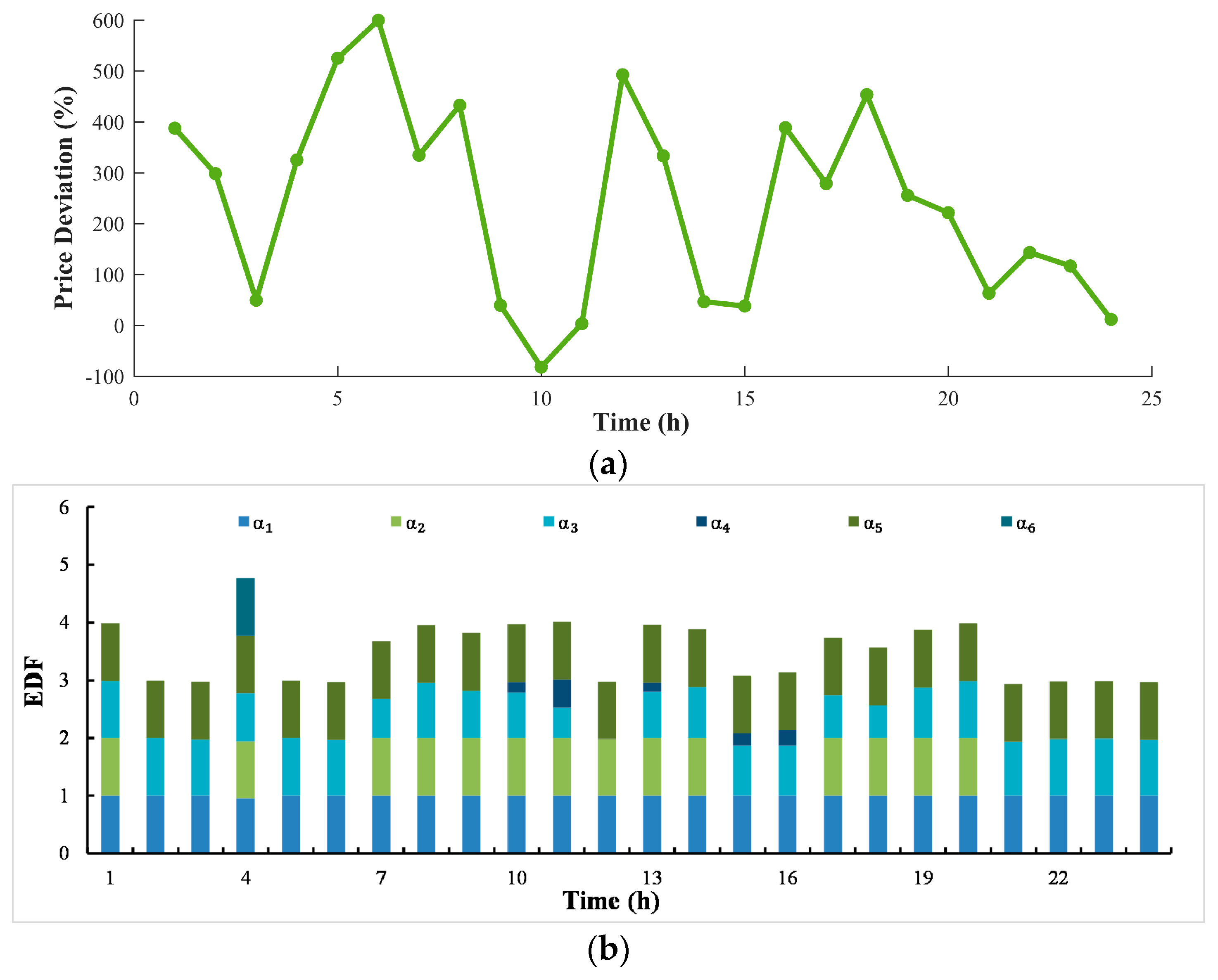
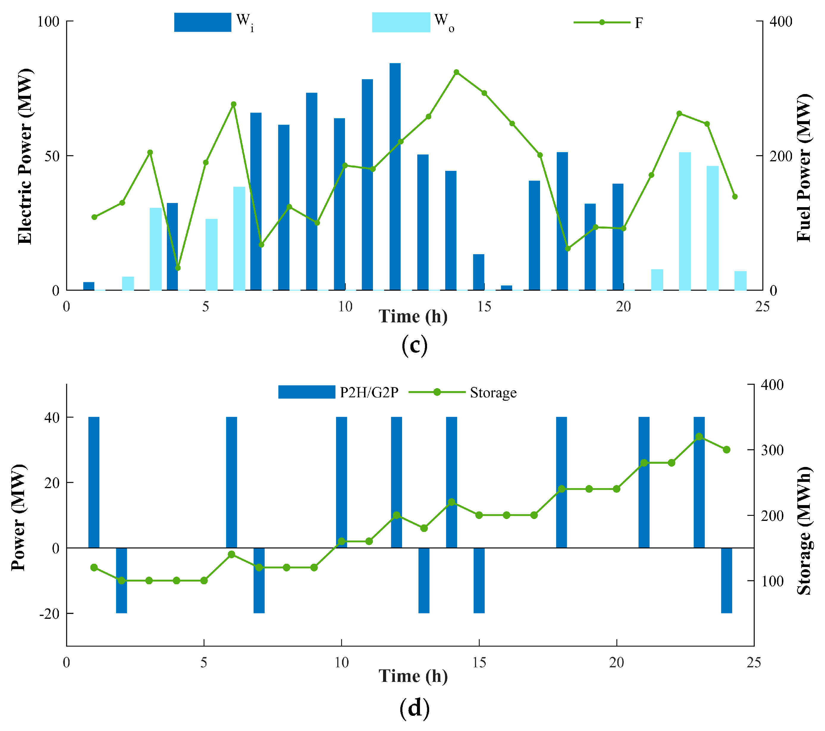
Due to the limitation of paper length, we took one out of the 100 optimized results for Scenario 3 for illustration purposes. The EV charging price is illustrated in Figure 16a; the EDF, input and output of the CCHP plant are illustrated in Figure 16b,c respectively; the input and output of the P2H/G2P plant are illustrate in Figure 16d.
With Case B, we may clearly see that the proposed optimal energy management method effectively facilitates the coordinated operation of ME applications, and contributes to the significant improvement of the profits, RES utilization, and energy saving performance of the MES.
5. Conclusions
In this work, a novel optimal energy management framework for the MES with multiple ME applications is presented, aiming at facilitating the coordinated operation of ME applications and improving the economic benefits, the ability in accommodating RES, and energy saving performance of the MES at the same time. In particular, the energy management models of CCHP plants, P2H/G2P plants, and the demand side management of the EV charging loads are integrated in the holistic energy management model of the MES. It will shed some lights on energy management studies of a system with multiple types of applications that have different operation mechanisms, such as a MES that is deployed with multiple types of ME applications, especially on facilitating their coordinated operation and promoting the operation performance of the entire system.
Author Contributions
Conceptualization, Y.W. and K.Z.; methodology, Y.W. and C.Z.; writing—original draft preparation, Y.W. and H.C.; writing—review and editing, Y.W., K.Z., H.C. and C.Z.
Funding
This research received no external funding.
Conflicts of Interest
The authors declare no conflict of interest.
Nomenclature
| A. CCHP plant | |
| Fi, Fo | Fuel thermal energy input/output (MW) |
| Wi, Wo | Electricity input/output (MW) |
| Qi, Qo | Heat input/output (MW) |
| Ri, Ro | Cooling power input/output (MW) |
| H | Efficiency matrix of CCHP plant |
| ηFF, ηFW, ηFQ, ηFR, ηWF, ηWW, ηWQ, ηWR, ηQF, ηQW, ηQQ, ηQR, ηRF, ηRW, ηRQ, ηRR | Entires in H (subscripts denote the type of energy outputs and energy inputs) |
| α | EDF array of CCHP plant |
| ηW, ηQ | Efficiency of CHP for electricity and heat production |
| ηt | Efficiency of CHG |
| COPQ, COPR | Coefficient of performance of EP for heat and cooling power production |
| μEP | The proportion of electricity input for heat production |
| COPWARG | Coefficient of performance of WARG |
| QDump | Dumped Heat of CCHP plant (MW) |
| B. P2H/G2P plant | |
| I | Operation mode indicator |
| PHdr | Output of P2H/G2P plant (MW) |
| ηG2P, ηP2H | Conversion efficiencies of G2P and P2H processes |
| , , , | Lower and upper output limits of P2H/G2P plants in G2P and P2H processes (MW) |
| Hsto | Storage level of P2H/G2P plant (MW·h) |
| , | Lower and upper storage limits (MW·h) |
| Hoth | Hydrogen power demand of other sectors (MW) |
| Upper limits of Hoth (MW) | |
| C. Demand response of EV | |
| Dev,i | Electricity consumption in period i (MW) |
| ρi | Electricity price in period i ($) |
| εii | Self-elasticity coefficient in period i |
| εij | Cross-elasticity coefficient between period i and period j |
| ΔDev,i, Δρi | Electricity consumption change (MW), price change ($) in period i |
| Dev,h, Dev,f, Dev,v | Electricity consumption during peak, flat and valley periods (MW) |
| ρh, ρf, ρv | Electricity price during peak, flat, and valley periods ($) |
| kh, bh, kf, bf, kv, bv | Factors used to describe the linearized relationships between electricity Consumption and price during peak, flat, and valley periods |
| ΩH, ΩF, ΩV | Peak, flat, and valley periods sets |
| ρTOU, ρ0 | Base electricity price array and TOU price ($) |
| D. Energy management model | |
| V | Decision variable vector |
| Fi | Objective function i |
| PG | Output array of generators (MW) |
| PHdr | Output array of P2H/G2P plants (MW) |
| ΩB, ΩG, ΩR | Buses, generators and RES set |
| ΩChr, ΩHdr, ΩCCHP | EV charging facilities, P2H/G2P and CCHP plants set |
| PG | Outputs of generators (MW) |
| PP2H/PG2P | Outputs of P2H/G2P plants in P2H/G2P mode (MW) |
| a, b, c | Consumption characteristics of generators |
| bP2H, cP2H, aG2P, bG2P, cG2P | Consumption characteristics of P2H/G2P plants |
| D | Electric load (MW) |
| PChr | EV charging load (MW) |
| Selling price of electricity ($) | |
| TOU EV charging price ($) | |
| Fuel price for electricity production ($) | |
| Fuel price for heat and cooling power production ($) | |
| PR | RES outputs (MW) |
| PR_max | Maximal RES outputs (MW) |
| WCCHP, QCCHP, RCCHP | Electricity, heat, and cooling output of CCHP plants (MW) |
| ηF | Fuel Thermal energy rate |
| PG, QG | Active and reactive power outputs of generators (MW) |
| PL, QL | Active and reactive demands (MW) |
| U, θ | Bus voltage magnitude and voltage angle |
| G, B | Conductance and reactance in admittance matrix |
| Sij | Apparent power between bus i and bus j (MVA) |
| , , , | Input and output limits of ME device x (MW) |
| , | ME input and ME demands of the CCHP plant m (MW) |
| ME exchange between CCHP plant m and external ME distribution networks (MW) | |
| , | Limits of EV charging price |
| Maximum EV charging load (MW) | |
References
- Mancarella, P.; Andersson, G.; Peças-Lopes, J.A.; Bell, K.R.W. Modelling of integrated multi-energy systems: Drivers, requirements, and opportunities. In Proceedings of the 2016 Power Systems Computation Conference (PSCC), Genoa, Italy, 20–24 June 2016; pp. 1–22. [Google Scholar]
- Bao, Z.; Zhou, Q.; Yang, Z.; Yang, Q.; Xu, L.; Wu, T. A Multi Time-Scale and Multi Energy-Type Coordinated Microgrid Scheduling Solution—Part I: Model and Methodology. IEEE Trans. Power Syst. 2015, 30, 2257–2266. [Google Scholar] [CrossRef]
- Clegg, S.; Mancarella, P. Integrated Electrical and Gas Network Flexibility Assessment in Low-Carbon Multi-Energy Systems. IEEE Trans. Sustain. Energy 2016, 7, 718–731. [Google Scholar] [CrossRef]
- Strbac, G. Integrating renewable energy to the grid optimising and securing the network: Facilitating cost effective integration of renewable energy in GB grid. In IET Seminar on Integrating Renewable Energy to the Grid: Optimising and Securing the Network; IET: London, UK, 2014; pp. 1–22. [Google Scholar]
- Olatomiwa, L.; Mekhilef, S.; Ismail, M.S.; Moghavvemi, M. Energy management strategies in hybrid renewable energy systems: A review. Renew. Sustain. Energy Rev. 2016, 62, 821–835. [Google Scholar] [CrossRef]
- Chen, Y.B.; Wang, Y.Z.; Ma, J. Multi-Objective Optimal Energy Management for the Integrated Electrical and Natural Gas Network with Combined Cooling, Heat and Power Plants. Energies 2018, 11, 734. [Google Scholar] [CrossRef] [Green Version]
- Mancarella, P.; Chicco, G. Integrated energy and ancillary services provision in multi-energy systems. In Proceedings of the 2013 IREP Symposium Bulk Power System Dynamics and Control—IX Optimization, Security and Control of the Emerging Power Grid, Rethymno, Greece, 25–30 August 2013; pp. 1–19. [Google Scholar]
- Zhang, R.; Jiang, T.; Li, G.; Chen, H.; Li, X.; Bai, L.; Cui, H. Day-ahead scheduling of multi-carrier energy systems with multi-type energy storages and wind power. CSEE J. Power Energy Syst. 2018, 4, 283–292. [Google Scholar] [CrossRef]
- Ivanova, P.; Sauhats, A.; Linkevics, O. District Heating Technologies: Is It Chance for CHP Plants in Variable and Competitive Operation Conditions? IEEE Trans. Ind. Appl. 2018. [Google Scholar] [CrossRef]
- Ban, M.F.; Yu, J.L.; Shahidehpour, M.; Yao, Y.Y. Integration of power-to-hydrogen in day-ahead security-constrained unit commitment with high wind penetration. J. Mod. Power Syst. Clean Energy 2017, 5, 337–349. [Google Scholar] [CrossRef]
- Shao, C.; Wang, X.; Wang, X.; Du, C.; Dang, C.; Liu, S. Cooperative Dispatch of Wind Generation and Electric Vehicles with Battery Storage Capacity Constraints in SCUC. IEEE Trans. Smart Grid 2014, 5, 2219–2226. [Google Scholar] [CrossRef]
- Siano, P. Demand response and smart grids—A survey. Renew. Sustain. Energy Rev. 2014, 30, 461–478. [Google Scholar] [CrossRef]
- Mancarella, P. From Cogeneration to Trigeneration: Energy Planning and Evaluation in a Competitive Market Framework. Ph.D. Thesis, Politecnico di Torino, Turin, Italy, 2006. [Google Scholar]
- Chicco, G.; Mancarella, P. Enhanced Energy Saving Performance in Composite Trigeneration Systems. In Proceedings of the 2007 IEEE Lausanne Power Tech, Lausanne, Switzerland, 1–5 July 2007; pp. 1423–1428. [Google Scholar]
- Schiebahn, S.; Grube, T.; Robinius, M.; Tietze, V.; Kumar, B.; Stolten, D. Power to gas: Technological overview, systems analysis and economic assessment for a case study in Germany. Int. J. Hydrog. Energy 2015, 40, 4285–4294. [Google Scholar] [CrossRef]
- Guandalini, G.; Campanari, S.; Romano, M.C. Comparison of gas turbines and power-to-gas plants for Improved Wind Park Energy dispatchability. In Proceedings of the ASME Turbo Expo 2014: Turbine Technical Conference and Exposition, Düsseldorf, Germany, 16–20 June 2014. [Google Scholar]
- Guandalini, G.; Campanari, S.; Romano, M.C. Power-to-gas plants and gas turbines for improved wind energy dispatchibility: Energy and economic assessment. Appl. Energy 2015, 147, 117–130. [Google Scholar] [CrossRef]
- Zhang, X.; Shahidehpour, M.; Alabdulwahab, A.; Abusorrah, A. Optimal Expansion Planning of Energy Hub with Multiple Energy Infrastructures. IEEE Trans. Smart Grid 2015, 6, 2302–2311. [Google Scholar] [CrossRef]
- Song, Y.H.; Yang, X.; Lu, Z.X. Integration of plug-in hybrid and electric vehicles: Experience from China. In Proceedings of the 2010 IEEE Power Engineering Society General Meeting, Providence, RI, USA, 25–29 July 2010; pp. 1–5. [Google Scholar]
- Ferdowsi, M. Vehicle Fleet as a distributed energy storage system for the power grid. In Proceedings of the 2009 IEEE Power Engineering Society General Meeting, Calgary, AB, Canada, 26–30 July 2009; pp. 1–2. [Google Scholar]
- De Forest, N.; Funk, J.; Lorimer, A.; Ur, B.; Sidhu, I.; Kaminsky, P.; Tenderich, B. Impact of Widespread Electric Vehicle Adoption on the Electrical Utility Business–Threats and Opportunities. University of California: Berkeley. Available online: http:// cet.berkeley.edu/dl/Utilities_Final_8-31-09.pdf (accessed on 28 September 2018).
- Yu, R.; Zhong, W.; Xie, S.; Yuen, C.; Gjessing, S.; Zhang, Y. Balancing Power Demand Through EV Mobility in Vehicle-to-Grid Mobile Energy Networks. IEEE Trans. Ind. Inform. 2016, 12, 79–90. [Google Scholar] [CrossRef]
- Sarker, M.R.; Ortega-Vazquez, M.A.; Kirschen, D.S. Optimal Coordination and Scheduling of Demand Response via Monetary Incentives. IEEE Trans. Smart Grid 2015, 6, 1341–1352. [Google Scholar] [CrossRef]
- Xu, Z.W.; Hu, Z.C.; Song, Y.H.; Zhang, H.C.; Chen, X.S. Coordinated Charging Strategy for PEV Charging Stations Based on Dynamic Time-of-use Tariffs. Proc. CSEE 2014, 34, 3638–3646. [Google Scholar]
- Chen, C.Y.; Hu, B.; Xie, K.G.; Wan, L.Y.; Xiang, B. A Peak-Valley TOU Price Model Considering Power System Reliability and Power Purchase Risk. Power Syst. Technol. 2014, 38, 2141–2148. [Google Scholar]
- Deb, K.; Pratap, A.; Agarwal, S.; Meyarivan, T. A fast and elitist multi-objective genetic algorithm: NSGA-II. IEEE Trans. Evol. Comput. 2002, 6, 182–197. [Google Scholar] [CrossRef]
- Harvey, L.D.D. A Handbook on Low-Energy Buildings and District-Energy Systems: Fundamentals, Techniques and Examples; Routledge: London, UK, 2012; ISBN 978-184407-243-9. [Google Scholar]
- Kirschen, D.S.; Strbac, G.; Cumperayot, P.; Mendes, D.D. Factoring the elasticity of demand in electricity prices. IEEE Trans. Power Syst. 2000, 15, 612–617. [Google Scholar] [CrossRef]
- Safdarian, A.; Fotuhi-Firuzabad, M.; Lehtonen, M. A Medium-Term Decision Model for DisCos: Forward Contracting and TOU Pricing. IEEE Trans. Power Syst. 2015, 30, 1143–1154. [Google Scholar] [CrossRef]
- Wood, A.J.; Wollenberg, B.F.; Wiley, J. Power Generation, Operation, and Control; Wiley-Interscience: Hoboken, NJ, USA, 1996. [Google Scholar]
Figure 1.
Energy input and output of typical multi-energy (ME) devices. CCHP: combined cooling, heat, and power; CHP: combined heat and power units; CHG: combustion heat generators; CERG: compression electric refrigeration generators; EP: electrical heat pumps; GARC: gas absorption refrigerator generators; WARG: water adsorption refrigeration generators; COP: coefficient of performance.
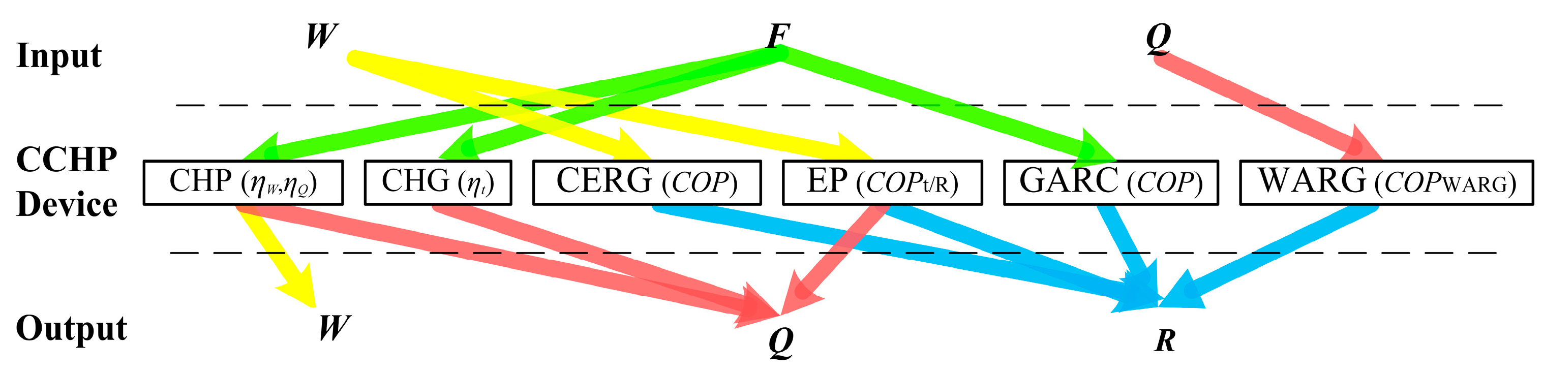
Figure 2.
The diagram of a typical combined cooling, heat, and power (CCHP) plant.
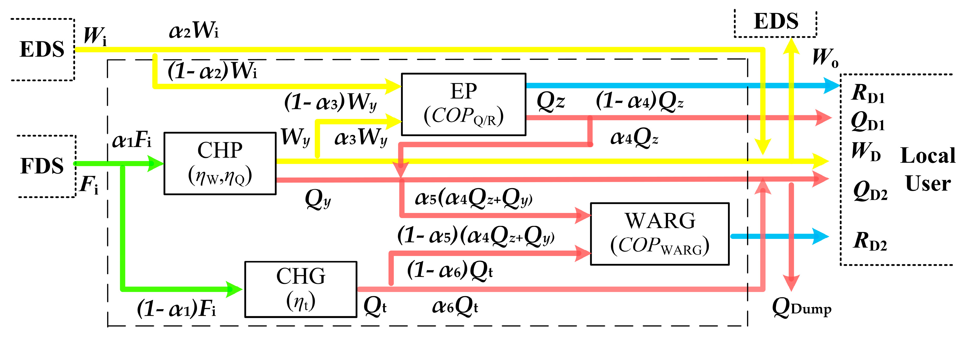
Figure 3.
Schematic of P2H/G2P concept. P2H/G2P: Power-to-Hydrogen and Gas-to-Power.
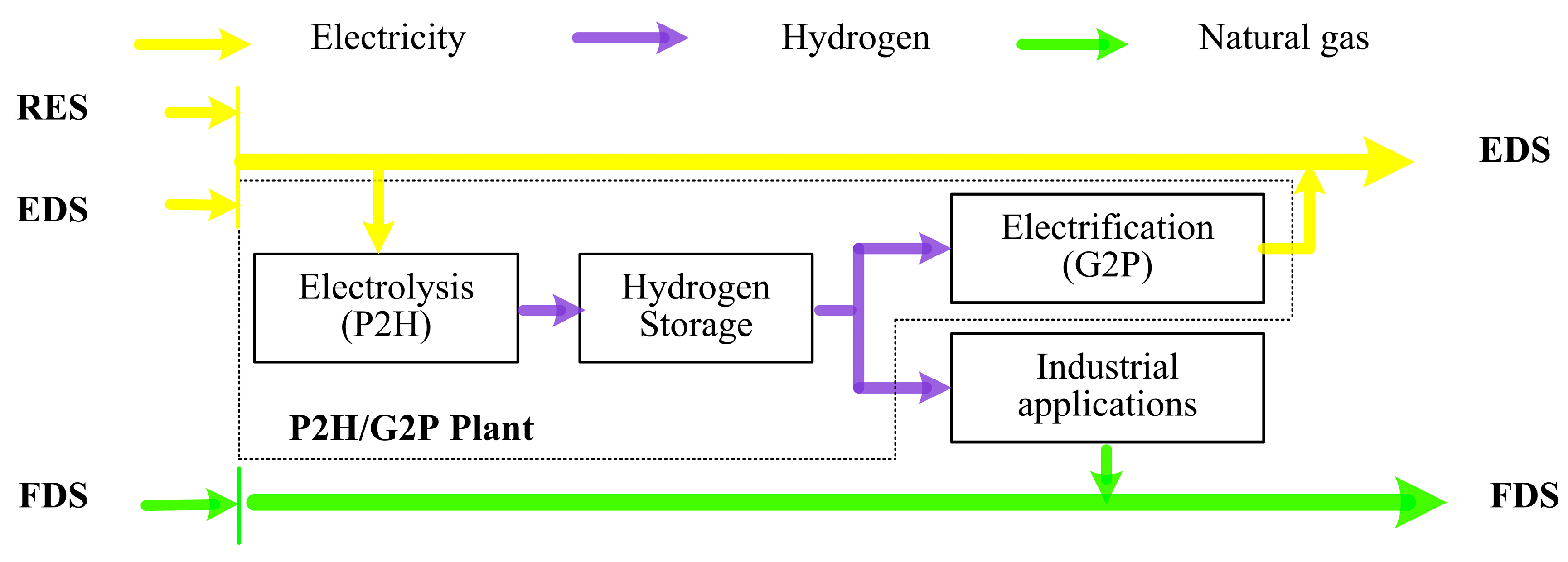
Figure 4.
The diagram of accommodating wind power with P2H/G2P.
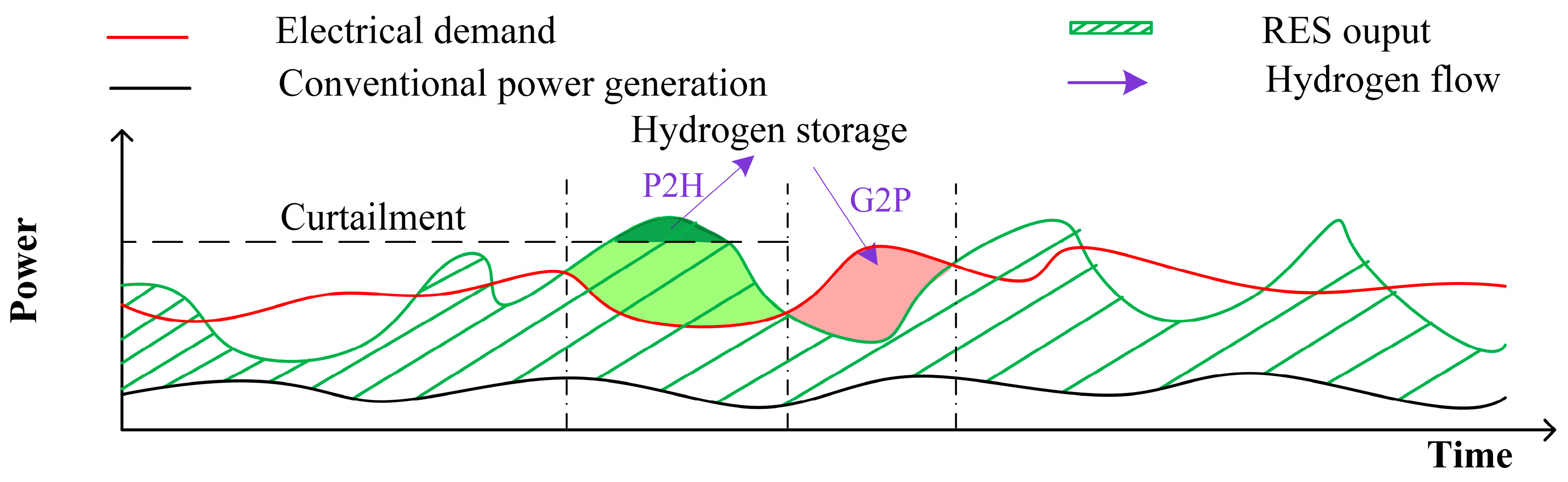
Figure 5.
Computation flow chart.

Figure 6.
Example six-bus power system. EV: Electric Vehicle.
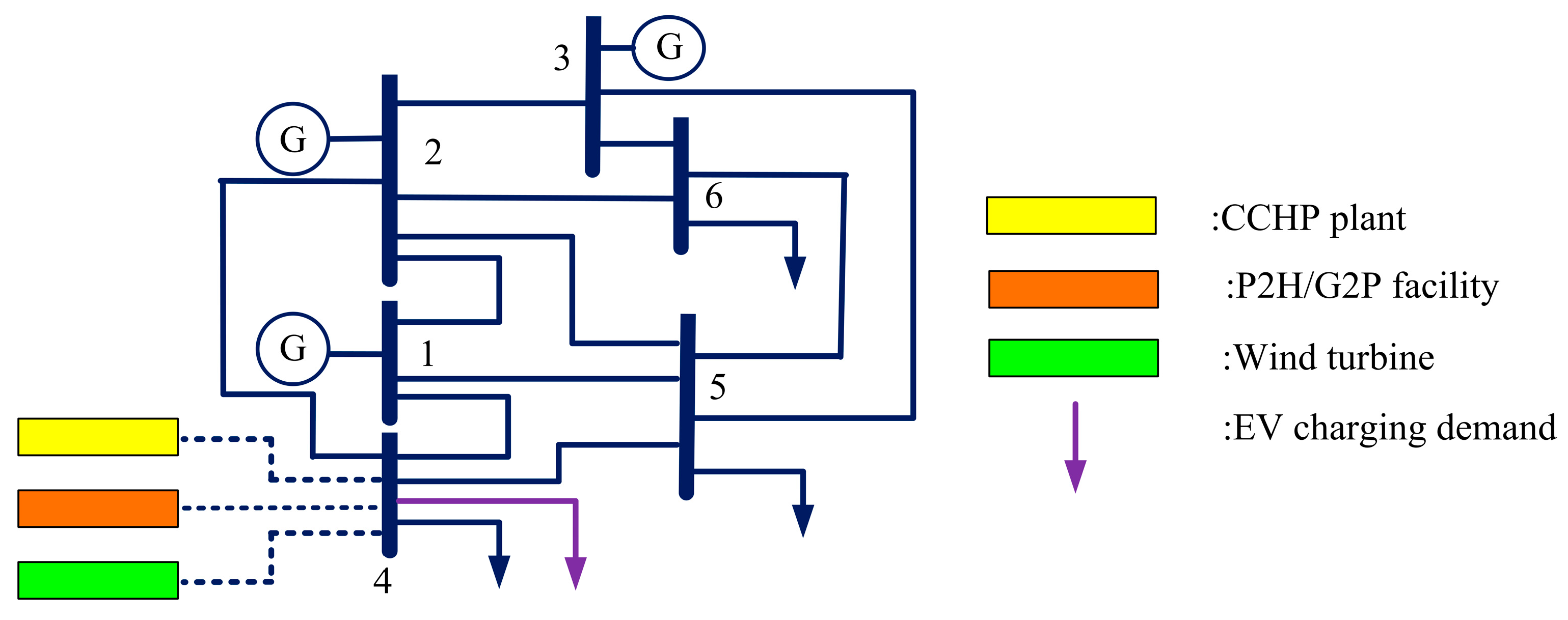
Figure 7.
Hourly forecasted wind power and demand distribution. (a) Forecasted wind power and electric demand. (b) Multi-energy demand.
Figure 7.
Hourly forecasted wind power and demand distribution. (a) Forecasted wind power and electric demand. (b) Multi-energy demand.

Figure 8.
Dispatch result in Case 1.

Figure 9.
Dispatch result in Case 2. (a) Outputs of conventional generators and the wind turbine. (b) Input and output of the CCHP plan.
Figure 9.
Dispatch result in Case 2. (a) Outputs of conventional generators and the wind turbine. (b) Input and output of the CCHP plan.
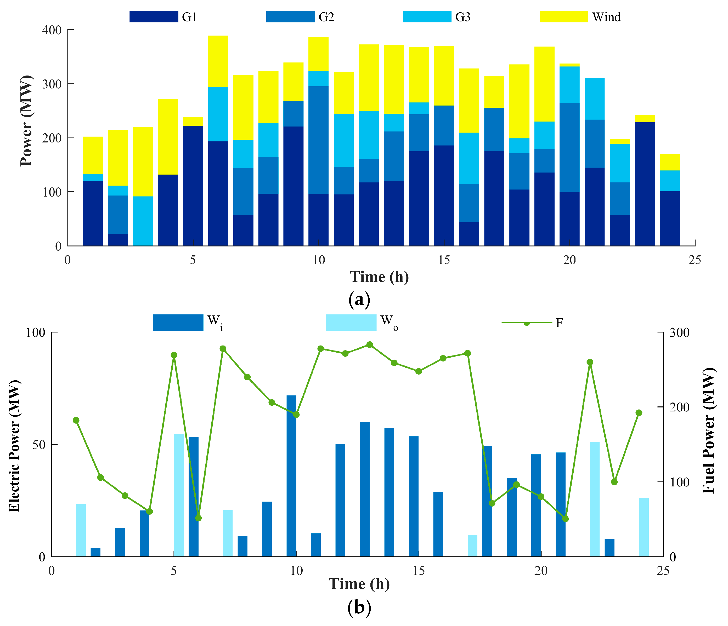
Figure 10.
Dispatch result in Case 3. (a) Outputs of conventional generators and the wind turbine. (b) Output of the P2H/G2P plant.
Figure 10.
Dispatch result in Case 3. (a) Outputs of conventional generators and the wind turbine. (b) Output of the P2H/G2P plant.
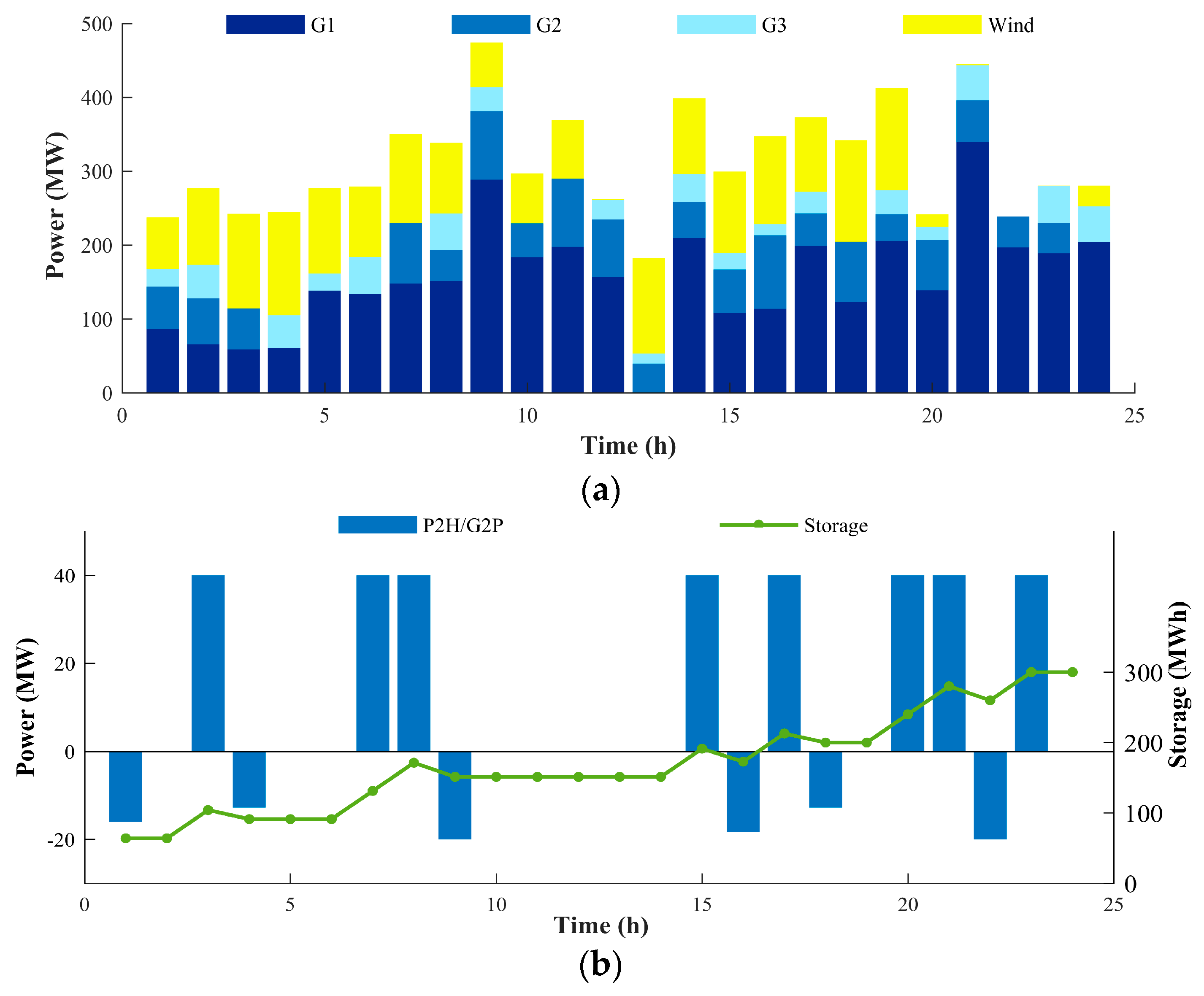
Figure 11.
Dispatch result in Case 4. (a) Outputs of conventional generators and the wind turbine. (b) Price deviation for EV charging.
Figure 11.
Dispatch result in Case 4. (a) Outputs of conventional generators and the wind turbine. (b) Price deviation for EV charging.
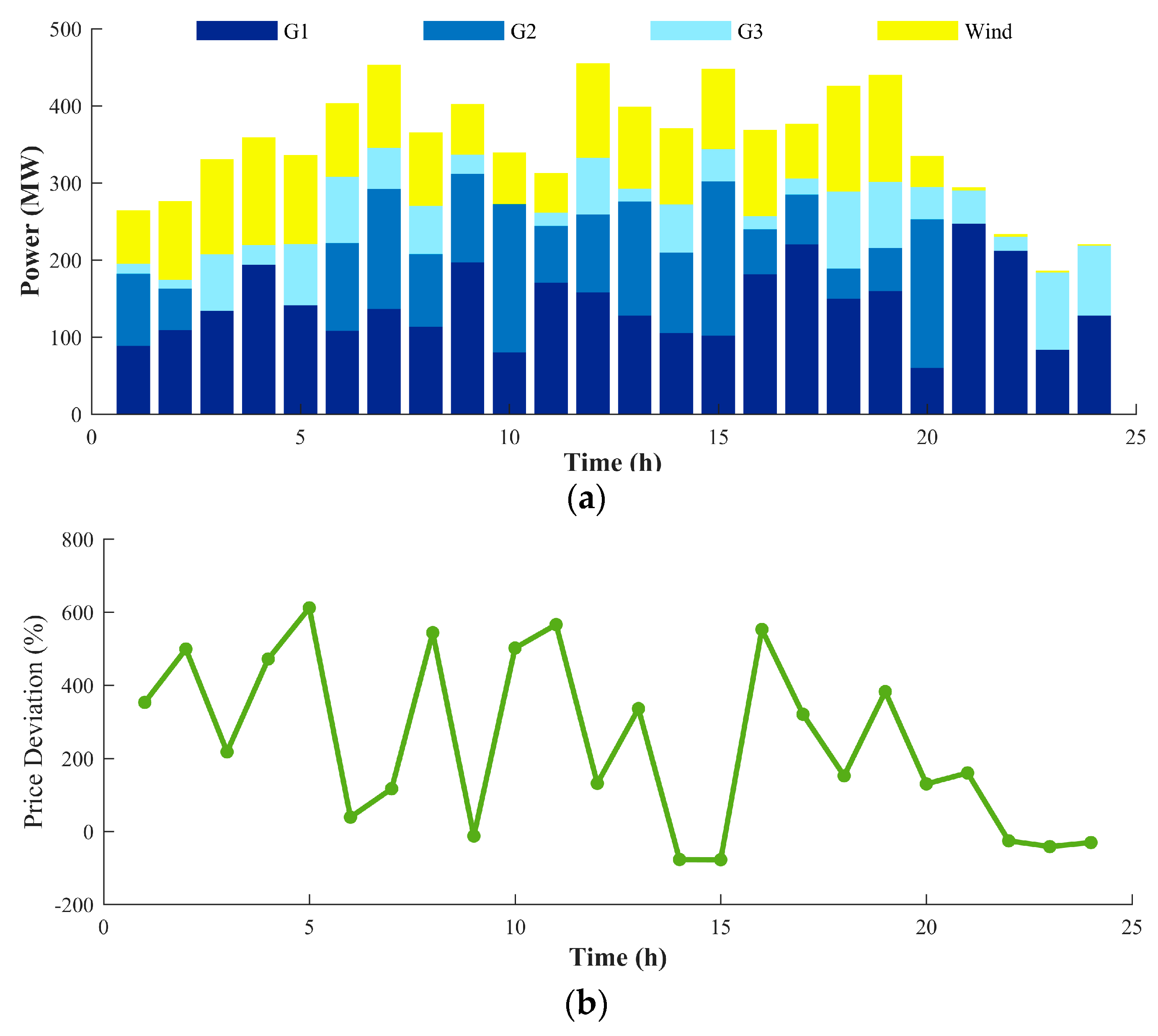
Figure 12.
Dispatch result in Case 5 and Case 6. (a) Outputs of conventional generators and the wind turbine. (b) Price deviation for EV charging. (c) Input and output of CCHP plant in Case 5. (d) Input and output of CCHP plant in Case 6.
Figure 12.
Dispatch result in Case 5 and Case 6. (a) Outputs of conventional generators and the wind turbine. (b) Price deviation for EV charging. (c) Input and output of CCHP plant in Case 5. (d) Input and output of CCHP plant in Case 6.
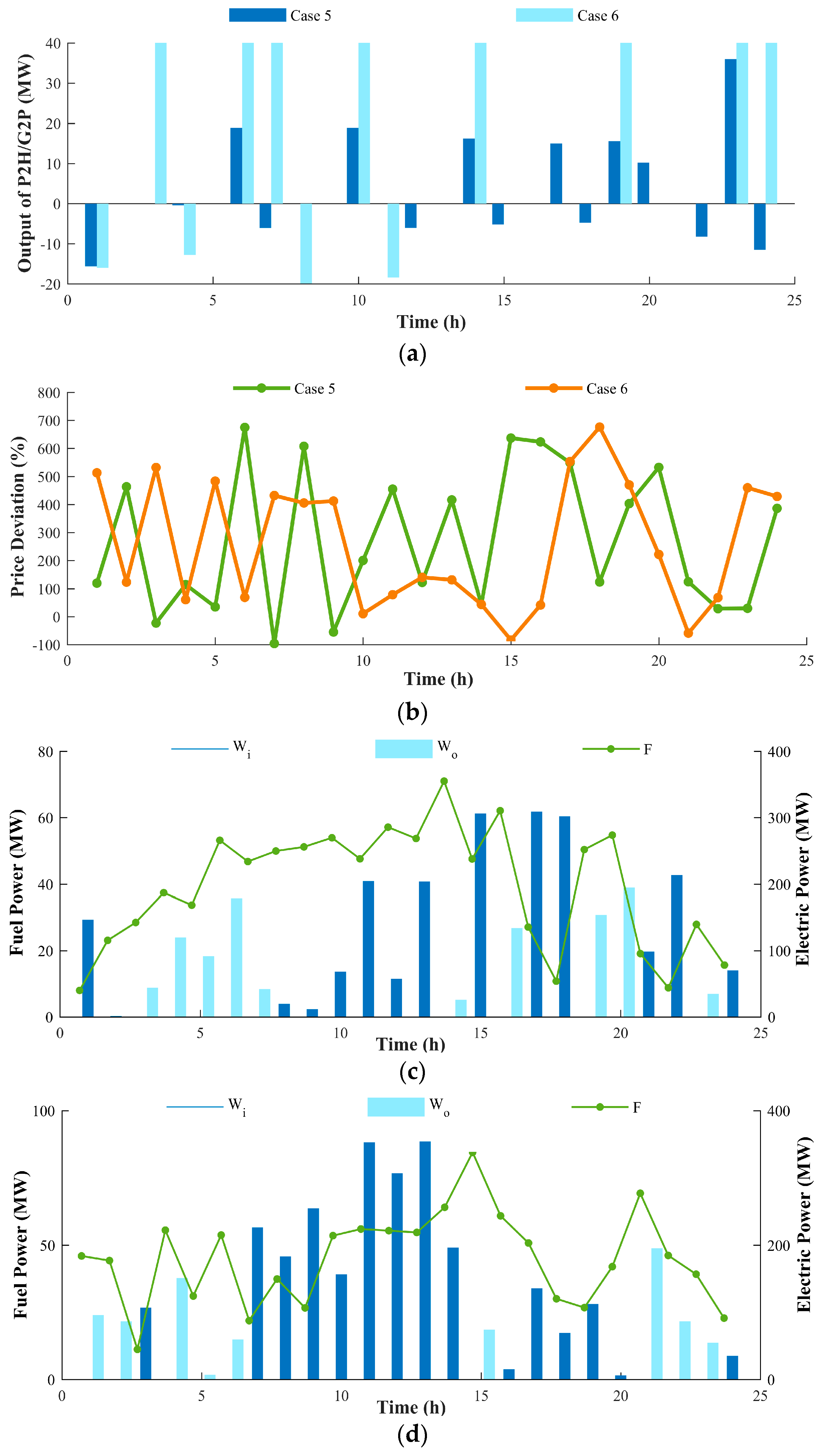
Figure 13.
Performance of the dispatch schemes in Case 1–6.

Figure 14.
The diagram of the modified IEEE 39-bus case.
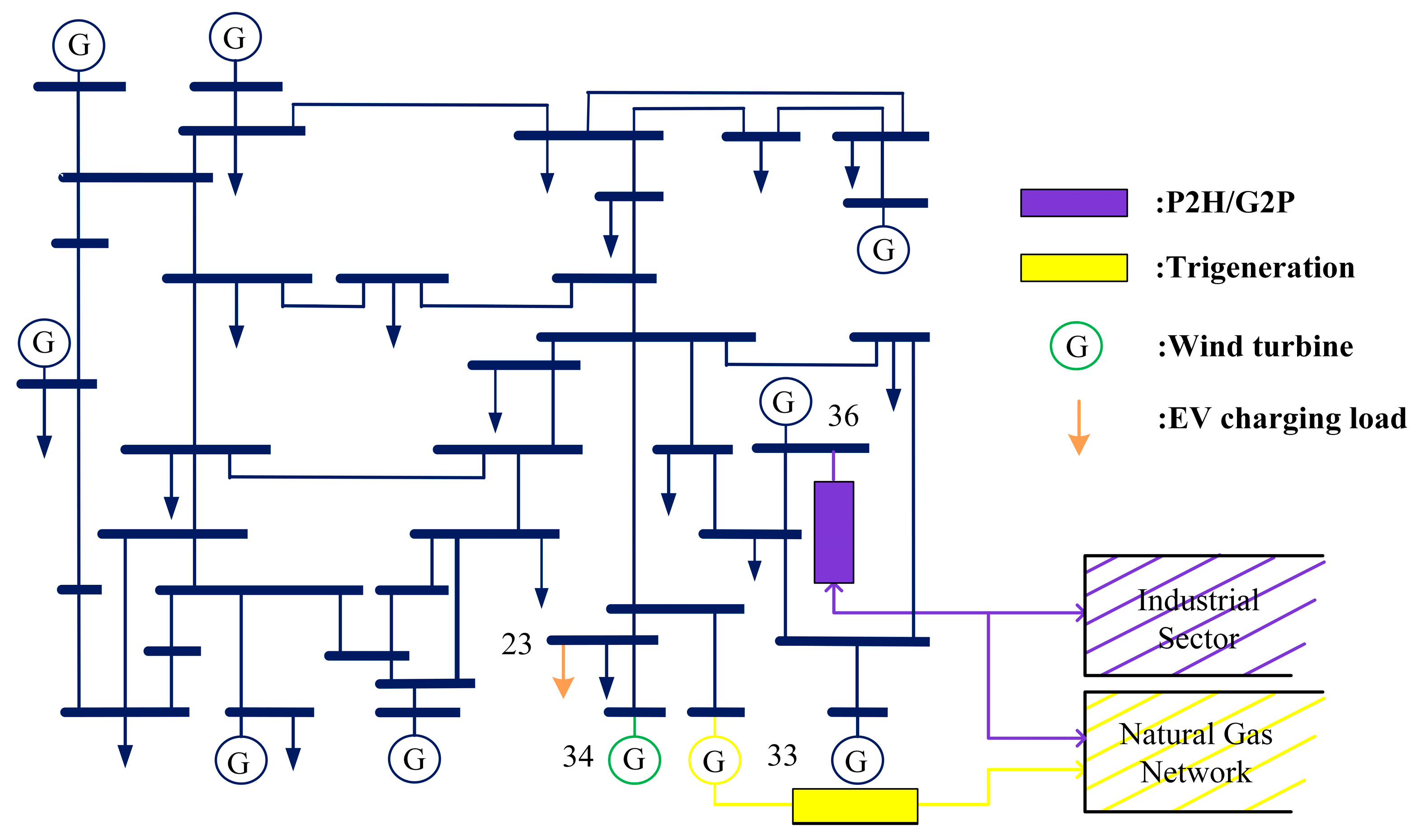
Figure 15.
Optimization result of Case B.
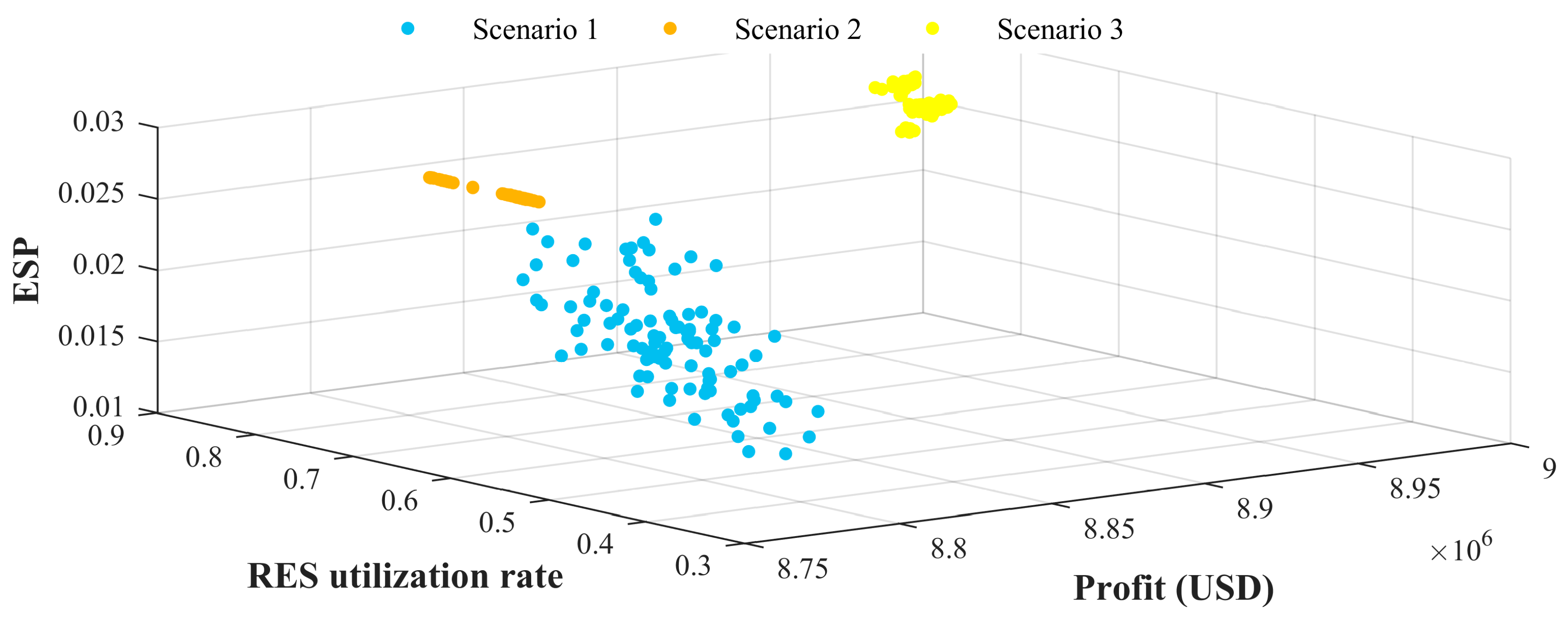
Figure 16.
The detailed optimized dispatch result. (a) Deviation of EV charging price. (b) EDF of the CCHP plant. (c) Input and output of the CCHP plant. (d) The dispatch result of P2H/G2P plant.
Figure 16.
The detailed optimized dispatch result. (a) Deviation of EV charging price. (b) EDF of the CCHP plant. (c) Input and output of the CCHP plant. (d) The dispatch result of P2H/G2P plant.

Table 1.
Generation unit characteristics 1.
| Unit | a (MBtu/MW2h) | b (MBtu/MWh) | c (MBtu) |
|---|---|---|---|
| G1 | 0.0004 | 13.5 | 176.9 |
| G2 | 0.001 | 32.6 | 129.9 |
| G3 | 0.006 | 17.6 | 137.4 |
| P2H | - | 12.5 | 141 |
| G2P | 0.0065 | 19.6 | 141.4 |
Table 2.
Generation unit characteristics 1.
| Unit | Pmax (MW) | Pmin (MW) | γ (CNY/MBtu) | Ton (h) | Toff (h) |
|---|---|---|---|---|---|
| G1 | 700 | 100 | 8.1049 | 1 | 1 |
| G2 | 250 | 30 | 8.0997 | 2 | 3 |
| G3 | 200 | 10 | 8.1003 | 1 | 1 |
| P2H | 40 | 10 | 0.065 | 1 | 1 |
| G2P | 20 | 10 | 8.125 | 1 | 1 |
Table 3.
Generation unit characteristics 2.
| ME Device | Efficiency | Capacity |
|---|---|---|
| CHP | ηW = 36% | 300 MW |
| ηQ = 43% | ||
| CHG | = 90% | 650 MW |
| EHP | COP = 3.5 | 150 MW |
| WARG | COPWARG = 0.65 | 800 MW |
Table 4.
Case design.
| Case Num. | Wind Power | CCHP | P2H/G2P | Demand Response of EVs |
|---|---|---|---|---|
| 1 | √ | × | × | × |
| 2 | √ | √ | × | × |
| 3 | √ | × | √ | × |
| 4 | √ | × | × | √ |
| 5&6 | √ | √ | √ | √ |
© 2018 by the authors. Licensee MDPI, Basel, Switzerland. This article is an open access article distributed under the terms and conditions of the Creative Commons Attribution (CC BY) license (http://creativecommons.org/licenses/by/4.0/).
Share and Cite
MDPI and ACS Style
Wang, Y.; Zhang, K.; Zheng, C.; Chen, H. An Optimal Energy Management Method for the Multi-Energy System with Various Multi-Energy Applications. Appl. Sci. 2018, 8, 2273. https://doi.org/10.3390/app8112273
AMA Style
Wang Y, Zhang K, Zheng C, Chen H. An Optimal Energy Management Method for the Multi-Energy System with Various Multi-Energy Applications. Applied Sciences. 2018; 8(11):2273. https://doi.org/10.3390/app8112273
Chicago/Turabian StyleWang, Yangzi, Kai Zhang, Chun Zheng, and Huiyuan Chen. 2018. "An Optimal Energy Management Method for the Multi-Energy System with Various Multi-Energy Applications" Applied Sciences 8, no. 11: 2273. https://doi.org/10.3390/app8112273
Note that from the first issue of 2016, this journal uses article numbers instead of page numbers. See further details here.