Detection of Defects Using Spatial Variances of Guided-Wave Modes in Testing of Pipes


1
Department of Electronic and Computer Engineering, Brunel University London, Uxbridge UB8 3PH, UK
2
NSIRC, Granta Park, Cambridge CB21 6AL, UK
3
TWI, Granta Park, Cambridge CB21 6AL, UK
*
Author to whom correspondence should be addressed.
Appl. Sci. 2018, 8(12), 2378; https://doi.org/10.3390/app8122378
Submission received: 19 October 2018
/
Revised: 13 November 2018
/
Accepted: 19 November 2018
/
Published: 24 November 2018
(This article belongs to the Special Issue Ultrasonic Guided Waves)
Abstract
:In the past decade, guided-wave testing has attracted the attention of the non-destructive testing industry for pipeline inspections. This technology enables the long-range assessment of pipelines’ integrity, which significantly reduces the expenditure of testing in terms of cost and time. Guided-wave testing collars consist of several linearly placed arrays of transducers around the circumference of the pipe, which are called rings, and can generate unidirectional axisymmetric elastic waves. The current propagation routine of the device generates a single time-domain signal by doing a phase-delayed summation of each array element. The segments where the energy of the signal is above the local noise region are reported as anomalies by the inspectors. Nonetheless, the main goal of guided-wave inspection is the detection of axisymmetric waves generated by the features within the pipes. In this paper, instead of processing a single signal obtained from the general propagation routine, we propose to process signals that are directly obtained from all of the array elements. We designed an axisymmetric wave detection algorithm, which is validated by laboratory trials on real-pipe data with two defects on different locations with varying cross-sectional area (CSA) sizes of 2% and 3% for the first defect, and 4% and 5% for the second defect. The results enabled the detection of defects with low signal-to-noise ratios (SNR), which were almost buried in the noise level. These results are reported with regard to the three different developed methods with varying excitation frequencies of 30 kHz, 34 kHz, and 37 kHz. The tests demonstrated the advantage of using the information received from all of the elements rather than a single signal.
1. Introduction
Pipelines are the main means of transferring oil and gas. They are usually installed in a hostile environment and suffer from defects such as corrosion or mechanical damage. To prevent the failure of pipelines, there is a need to inspect them in service in order to ensure their structural integrity. One of the many methods for the non-destructive testing of pipes is ultrasonic guided waves (UGW). This technology uses sets of transducer arrays to generate a low-frequency ultrasound signal. This ensures that elastic waves are guided through the boundary of the pipe; hence, the name guided waves [1]. Therefore, from one test point, the long-range inspection of pipelines is possible. However, the interoperation of UGW signals tends to be difficult due to the existence of the coherent noise in the tests.
Despite using arrays of transducers, UGW testing systems use a general routine process that outputs a single monodirectional signal in a time domain [2,3,4,5]. The generated signal is then used by inspectors to report any anomalies above the regional signal noise level [6]. To allow an ease of inspection, many types of research have been defined to use the characteristics of guided waves to increase the signal-to-noise ratio (SNR), increasing the defect detection accuracy.
One of the widely used techniques in the signal processing of guided waves is the work of Wilcox et al., which uses previously calculated dispersion curves in order to compensate for the effect of dispersion for the wave mode of interest in a certain propagation distance [7]. In 2013, Zeng et al. [8] used the basis of the dispersion compensation technique and introduced a novel method to design waveforms in order to pre-compensate for a certain propagation distance. Various researchers investigated the pulse compression approach, which consisted of exciting a known coded sequence and match-filtering the results in order to detect the known sequence [9,10,11,12]. Mehmet et al. [9,10] introduced an iterative dispersion compensation for removing the dispersion effect of guided-wave propagation. In 2016, Lin et al. [11] reported on the performance of different excitation sequences in terms of their ability to achieve δ-like correlation on Lamb waves. Most recently, Malo et al. [12] developed a two-dimensional compressed pulse analysis in order to enhance the achieved SNR of each wave mode. Coded waveform approaches have also been implemented in the enhancement of SNR in the inspection of Long Bones using guided waves [13]. In the pulse compression approaches, the results are always a trade-off between the spatial resolution and SNR; for having a high-energy, δ-like correlation result, the wavelength must be increased. Furthermore, the transfer function of the excitation system can affect the accuracy of the coded waveforms. These two factors mean that the initial waveform design and the accuracy of inspection using this method depend on the testing conditions. Furthermore, if non-dispersive regions of wave modes are used, there will be no need to use dispersion compensation algorithms.
Another method for filtering the guided waves signal is the work of Pedram et al. in Split-Spectrum Processing (SSP) [14,15], whereby through selecting the optimum filter parameters, the coherent noise of the test cases can be removed. However, automatic selection of the optimum filtering parameter is not possible at present. These parameters can be varying with regard to central excitation frequencies and the pipe geometries. On a similar note, frequency sweep examination, which was developed by Fateri et al. [16] in 2014, uses a similar concept in a way that defect features should exist in all of the frequency bands. Based on this fact, a novel method was developed that processes signals with different excitation frequencies, and is able to distinguish between the dispersive and non-dispersive wave modes that exist in the test. This method has never been tried in the pipes before, and requires many different excitations to be calculated on the same test subject. As it is currently known, due to backward cancellation algorithms and an overall system transfer function [4], it is not perfect, and not all of the frequencies can be used for optimum excitation (it can be varying depending on the pipe and tool set used). This will affect the accuracy of the algorithm if it is converted for pipeline inspection.
In 2015, Ching-Tin Ng [17] investigated signal processing approaches for the enhancement of results produced by guided-waves signals, in which he reported that Hilbert transform, Gabor wavelet transform, and discrete wavelet decomposition are able to improve the detectability of the results. UGWs have also been used for monitoring purposes. In 2015, Dobson et al. implemented independent component analysis (ICA) combined with previously developed temperature compensation methods [18,19] to enable the successful guided-wave monitoring of pipelines. In 2017, Chang et al. [20] introduced the idea of an adaptive sparse deconvolution method, with the aim of distinguishing the overlapping echoes of an ultrasonic guided-waves signal.
All of the algorithms have been developed with one purpose in mind: the improvement of the SNR to increase the possibility of the detection of a defect signal. However, the full potential of the system has not yet been established. The signal information in these systems are received from three rings of (at least) 24 transducers, but in the mentioned work, there is only one signal, which is achieved after the propagation routine of the device by summing the phase-delayed version of all of the transducers together. This routine was created to reduce the received flexural signals and have a unidirectional inspection [4,5]. Nonetheless, the received informatics can be processed in a better method, i.e., to use all of the available sensors for detecting the defect location rather than changing the information into a single time-domain signal.
On the other hand, array processing techniques that use individual signals are generally used for imaging and focusing applications [21,22,23,24,25,26,27]. However, these algorithms are computationally expensive, and might require the individual excitation of transducers [26], or a phased-array focusing of the transducers [23], rather than synthetic focusing, where all of the transducers in the array are excited at the same time [21]. This adds to the complexity of the interpreting the results. Furthermore, the goal of these algorithms is imaging a segment of the pipe rather than the detection of the defect location.
In this paper, we propose a new algorithm to solve the problem of detections, which can possibly be combined with all of the above-mentioned methods for SNR enhancement. The aim of this algorithm is to illustrate the possibility of using all of the individual transducers for defect detection instead of using a single signal achieved after the general routine. This way, both the spatial and temporal characteristics of the signal can be examined in more depth, which can lead to more accurate results. Furthermore, unlike imaging techniques, it uses normal excitation sequences, and thus can be applied to all of the data sequences, even if they are achieved in the past.
Section 2 explains the nature of noise on the guided-waves signal and the wave formation with regards to unique features. In Section 3, a novel method is proposed that uses the characteristic of axisymmetric waves to allow the detection of the defect signal. Validation was done by laboratory trials using two separate defect locations. The first defect is in a region where less coherent noise exists in the baseline with a varying size of 2% and 3% of the pipe’s cross-sectional area (CSA), and the second defect is located in higher spatial noise with a varying size of 4% and 5% CSA. The setup of these tests and the results are reported in sections 4 and 5, respectively. In the last section, a summary of current achievements as well as the further works is reported.
2. Background Theory
Guided waves are dispersive and multimodal [2]. Dispersion causes the energy of a signal to spread out in space and time as it propagates [7]. Guided wave modes are categorized based on their displacement patterns (mode shapes) within the structure. Three main families of waves exist in pipes, which are longitudinal, torsional, and flexural. Longitudinal and torsional waves are axisymmetric waves, while flexural waves are non-axisymmetric. The popular nomenclature used for them are in the format of X(n,m), where X can be replaced by the letters L for longitudinal, T for torsional, and F for flexural waves; n shows the harmonic variations of displacement and stress around the circumference, and m represents the order of existence of the wave mode [28].
Due to the sinusoidal and spatial variations of flexural waves, these coherent noises in the inspection can be reduced by adding the signals received from linearly spaced transducers around the circumference of the pipe. The resultant effect is the cancellation of non-axially symmetric flexural waves and the enhancement of axially symmetric torsional or longitudinal waves. However, cancellation is not ideal because of the imperfections of the real-world devices. These factors include the non-linear spacing of the transducer’s placement, the variability of the transducer’s frequency response, the number of transducers used, or the tolerances of the electronic test device. Furthermore, a scattering of an ideal axisymmetric wave with a non-axisymmetric feature would also result in the generation of other wave modes, which is commonly known as a wave mode conversion phenomenon [29,30,31,32]. Thus, inspecting guided waves without the interference of these coherent noises is near impossible.
For decades, the inspectors have been trained to interpret these resultant time-domain signals to extract the defect location. Nevertheless, the problem of detection can be defined in another way, i.e., the linearity and symmetry between the phases of the received waveforms. For better understating of this matter, in the following section, different conditions of waves arrived at spatially are demonstrated using a synthesized model.
2.1. Wave Formation
The scattered wave would consist of the excited axisymmetric and its associated flexural waves. Depending on the feature shapes, the energy distribution of each of the created wave modes would be different. As an example, a perfectly axisymmetric feature in the ideal scenario would result in the generation of a perfect axisymmetric response with no other flexural waves. In these scenarios, if the axisymmetric wave is stronger than the coherent regional noises in the area, an anomaly is reported by the inspectors. However, since it is a visual interpretation, in some scenarios, the resultant mixture of flexurals can easily lead to false alarms due to their coherence to the expected received signal. Furthermore, the axisymmetric wave can be smaller than the local noise level, and therefore would not be detected. These are some of the main challenges faced when inspecting the temporal domain.
Figure 1 shows the spatial arrival of the signals received from two rings of 32 source points. These signals are generated by the finite element model (FEM) [30]. In this setup, ideal source points are assumed, which leads to the generation of a perfect wave mode in all of the figures except (b) and (i), where the frequency response of each transducer is variable.
The red and blue signals are showing the first and second ring, respectively, and the reference is illustrated by the black dotted line. Thus, the values inside the reference would mean a negative phase, and values higher than the circle would mean a positive amplitude of the individual transducer.
2.1.1. Pipe End
The received signals from the pipe end are shown in Figure 1a–c. As can be seen in (a), a pure wave is generated, since both the excitation sequence and the feature are perfectly axisymmetric. However, in the cases of (b) and (c), where the flexurals are created by imperfect excitation and from wave mode conversion, respectively, the received response is the superposition of and flexural waves. The scattering from the pipe end would result in all of the energy of the wave to be reflected. Thus, a strong proportion of the received signal energy corresponds to the wave, and small variations are caused by flexural waves.
2.1.2. Defect
In cases (d)–(g) of Figure 1, the received waves is generated from a non-axisymmetric defect with a cross-sectional area size of 3%. The shown signals are different sequences from various times with respect to the temporal domain signal. The capture times are shown in Figure 2b where the red line is representing case (d), the blue line is representing case (e), and the green line is representing case (f). Case (g) is captured at the same time as case (e), but the generated wave is from a defect located at 0° (the right side of the pipe), while the other cases were from a defect angled at 90° (top side). Four important points are illustrated from the figures:
- Unlike the pipe end, defects that are non-axisymmetric features will inherently generate flexural waves. Nonetheless, the strongest energy will be associated with the T(0,1) wave.
- The end of the signal envelope will contain more flexural waves compared to the start of the envelope. At the start of the envelope, at most one cyclic variation will exist in the spatial domain, which would represent a low-order flexural wave mode. Nonetheless, near the end of the envelope, higher order variations (three or more) are starting to increase. This is because after the center of the envelope, the power of the T(0,1) wave is starting to decrease, and the higher order flexural with a lower travel speed is beginning to arrive.
- The strongest energy of the T(0,1) wave is associated with the peak of each cycle in the temporal domain, where most of the transducers will have the same phase.
- When the angle of the defect is changed, the direction of the arrival changes, but the phases and the overall formation of the wave remain the same.
2.1.3. Coherent Noise
The spatial arrival of the flexural noises created by the wave mode conversion and the backward leakage due to the imperfect excitation is shown in Figure 1h,i, respectively. Their corresponding time domain signals are shown in Figure 2b,c. As can be seen, for the flexural signal, the reception point phases are highly non-linear, which is completely different from the case of the defect signal.
Backward cancellation is not always perfect, due to the fixed ring spacing and the variance along the received waves from each transducer. In the temporal domain, these waves might still be detected, but when one looks at the phases between the two rings, it is observable that the two rings would have the exact opposite phases. Thus, it would be easier to detect signals received from the opposite direction in the spatial domain.
3. Methodology
In the previous section, it was demonstrated that in the case of flexural waves, high-order sinusoidal variation along the pipe’s circumference will be created. In ideal scenarios, where a perfect axisymmetric wave hits a perfect axisymmetric feature, the received amplitude in each transducer must be the same. However, due to the imperfections of the transducers and the testing conditions, there will be variance along each of the received amplitudes from the transducers; nonetheless, they all will have the same phase. Similar to the pipe ends, defects would generate a significant amount of torsional mode. However, they also do create flexurals with respect to the defect size and location. For signals coming from the backward direction, it is observed that the phases would practically be the inverse of each other for each transducer.
Based on these observations, by detecting the linearity between the phases of the sensors, the axisymmetric waves can be detected. Since not all of the phases would become the same in the case of defect signals, a measure of similarity between the phases must be defined, which can then be the threshold for detection.
3.1. General Routine
The first step in the general propagation routine of guided wave devices is to cancel the signal received from the backward direction. For doing so, the signals received from Ring 2 are initially subtracted from Ring 1 and Ring 3, and then the results are phase-delayed with respect to the tool set’s ring distancing and the excitation wave mode dispersion curve ( in this case). The results are stored in the matrix:
where represents the sample number, is the sensor number, and represents the total number of achieved signals, which is twice the number of transducers in each ring. This method will result in components to be overlapped. For the signals received from the forward test direction, this overlap will be positive, and for the backward direction, the amplitudes are inverted, which allows the unidirectional inspection. The temporal domain signal, which is generally used for inspection, is achieved by taking the mean of the :
3.2. Initialization
All of the transducers have the same phase when the sum of all of the signals from the same-phase transducers is equal to the sum of all of the signals. Therefore, the measure of similarity of the phases is defined by taking the difference between the sum of all of the signals and the sum of in-phase signals received from each transducer. The sign of the temporal domain demonstrates which sign is the greater power of iteration. Based on this sign, a mask is created for each transducer as follows:
Using this mask, in-phase signals with the temporal domain of each sample can be identified, and their sum can be calculated as:
Afterward, the similarity can be defined using:
3.3. Threshold Selection
In cases where a significant proportion of iterations energy is from the wavemode, the will be zero. However, as shown previously, defect signals will contain a mixture of flexural and torsional wave modes, leading this value to be non-zero. Hence, there is a need for defining a threshold for detecting the defects. In this section, three methods are presented defining this threshold.
3.3.1. Method One
In this method, a static constant is defined by the inspector. If the is less than this defined threshold, the sample would be marked as one, which means that a feature is detected; otherwise, it would be marked as zero:
For small signals, this formula would not be accurate, since inherently, their sum would be bigger than the threshold; thus, a compensation factor, 0.001, is added to prevent outliers from being detected in the noise region. This is an acceptable level, since the defect signals smaller than 0.001 would not be detected by the analog to digital converters of the device due to their limited discretization range. If the amplitude of the signal in the temporal domain is greater than this compensation factor, the algorithm would work as normal, else it would be zero:
The disadvantages of this method are that firstly, a user input is required, and secondly, the value is fixed for all of the features, disregarding the existing characteristics in each sample.
3.3.2. Method Two
To use signal characteristics more effectively, the amplitude of the signals can be used to define the threshold, since a greater signal can be the result of a greater linearity of the phases. By taking a percentage of the signals, a higher threshold can be assigned to such cases. In this method, a fixed percentage value needs to be set by the inspector, and the threshold for each iteration would be adaptively changed:
Another improvement to this algorithm would be to consider the effect of as well. A higher means that there is a higher chance that the signal is not linearly received by all of the transducers. This effect is significant in the case of signals received from the backward direction. In each iteration, the can be subtracted from the , which would decrease the resultant threshold value for backward propagating or non-axisymmetric waves:
3.3.3. Method Three
To eliminate the human error, the requested input from the user must be eliminated. The phases are the main factor in detecting the results; the percentage can be defined based on the ratio of the in-phase sensors over the total number of sensors:
In no iteration is the value of zero; it always have a positive offset, which means that the percentagecannot be replaced directly into Equation (8). Nonetheless, this offset can be removed by subtracting the mean of the calculated for all the samples from each individual sample:
where N is the total number of samples in the test. The final considered percentage for each sample would be:
Doing so removes the need for user input, and provides a more accurate thresholding with regard to the phases of the signals in each sample; the higher number of the same phase signals means a higher percentage value for the sample, which leads to a higher chance of detection. The formula for the first version (V1) and second version (V2) of this method can be achieved by substituting the new percentage achieved from Equation (12) in Equation (8) or Equation (9):
3.4. Limits Definitions
Three main detection limits exist in these algorithms. (1) The first if the , which is the minimum value required for each method to detect at least one cycle of the defect signal. (2) Second is the , which is the maximum allowable value for the methods to detect the defect without any outliers. By moving toward the value, the detection length increases; however, the accuracy reduces as the chance of detecting outliers increases. Thus, for comparing the methods together, an value is defined using the and . This value is the best possible compromise between the achieved defect length and the possibility of detecting false alarms. For method three, the average value is calculated using Equation (11), and and values are achieved by manually replacing the average in Equation (14). For both of the other methods, the average value is calculated manually from the achieved and values in the tests. Also, the margins are defined as the difference between the and , which illustrate the values where manual inputs will produce a result without any false alarms.
3.5. Program Flowchart
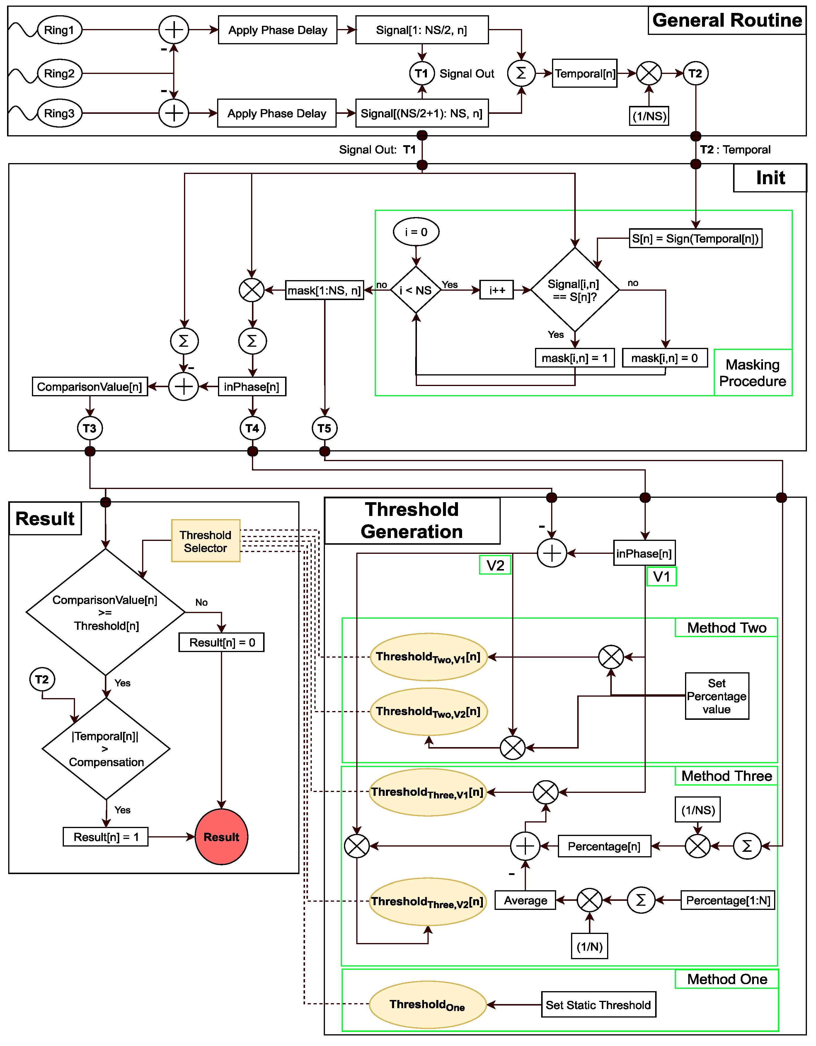
The program flowchart is shown in Figure 3. As can be seen, the three stages of general routine, initialization, and result generation are the same in all of the methods. However, the threshold value that is used in the result stage is selected based on methods one, two, or three, which are explained in the thresholding section.
4. Experimental Setup
The Teletest device [33], manufactured by Teletest branch of Eddify technology family in Cambridge (UK), used in order to inspect an eight-inch schedule 40 steel pipe with a length of six meters. The test tool included three rings of 24 linearly spaced transducers with 30-mm spacing, which are located 1.5 m away from the back end of the pipe. The main aim of these trials is to assess the ability of the algorithm in highly noisy scenarios and investigate the dependency of each method to the excitation frequency.
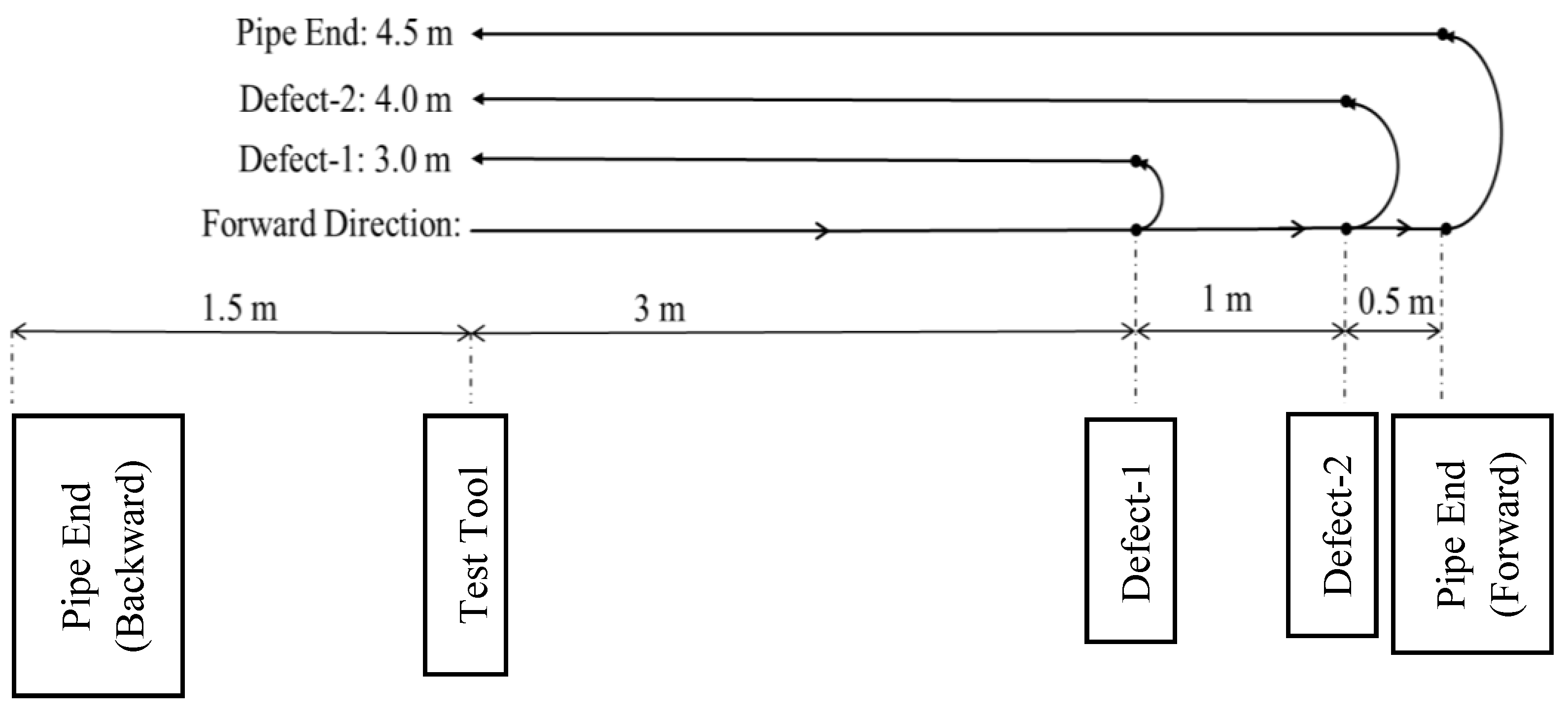
In the first set of tests, two defects of 3% and 2% CSA have been created; these are located 4.5 m from the back end of the pipe, which generates signals with less/almost the same energy as the noise regions. In order to confirm the ability of this thresholding method in detecting another defect in the same pipe, defects with CSA sizes of 4% and 5% have been created after the initial trials, which are located 5.5 m away from the back end of the pipe. Figure 4 shows the signal reception routes of this setup.
The excitation sequence is a 10 cycle Hann-windowed sine waves with frequencies of 30 kHz, 34 kHz, and 37 kHz. The selected frequencies are considered the optimum excitation sequences with regard to their resultant forward propagating energy achieved using the backward cancellation algorithm [30]. A summary of the settings used for the first set of tests (first defect), which are numbered from one to six, are shown in Table 1; for the second set of tests, they are numbered from seven to 12 (second defect), and are shown in Table 2.
Figure 5 shows the baseline signals achieved from the same pipe with no defects, with excitation frequencies of (a) 30 kHz; (b) 34 kHz; and (c) 37 kHz. As can be seen, even though there are no defects in the pipe, the baseline signal is highly polluted by the coherent noise. The first defect signal is expected to be received approximately three meters away from the tool test, between the first and second red dotted lines. The second defect is expected to be located approximately four meters away, between the third and fourth red dotted lines. Three major conclusions can be drawn with regard to the baselines:
- Defect 1: The signal with lowest amount of existing coherent noise in the baseline are 34 kHz, 30 kHz, and 37 kHz, respectively.
- Defect 2: The lowest amount of existing coherent noise in the baseline belongs to 37-kHz, 34-kHz, and 30-kHz signals, respectively
- All of the respective frequencies have a higher amount of noise in the Defect-2 region.
It is expected that the thresholds are required for detecting regions with lower existing coherent noises, which means that overall, Defect 2 will be more difficult to detect.
5. Results
In this section, the limits achieved for detecting the defect signal using each method is reported. The SNR of the defects in each test is demonstrated in Table 1. These values are generated using the following equation:
The SNRs are calculated with respect to the overall noises in the region. In the case of test numbers 1–6, only the energy of Defect 1 and the pipe end signal is removed for calculating the energy of the noise; however, for test numbers 7–12, as well as the Defect-1 and pipe end signals, the Defect-2 signal is also removed for calculating the noise. As demonstrated in Table 3, the defect signals are within the noise level, and identification of them using the inspection routine would not be accurate, especially for a 2% CSA defect. Nonetheless, the overall SNR of Defect 2 is much higher due to both the increment of CSA size, and the existing coherent noises of the region.
5.1. Example Test Case
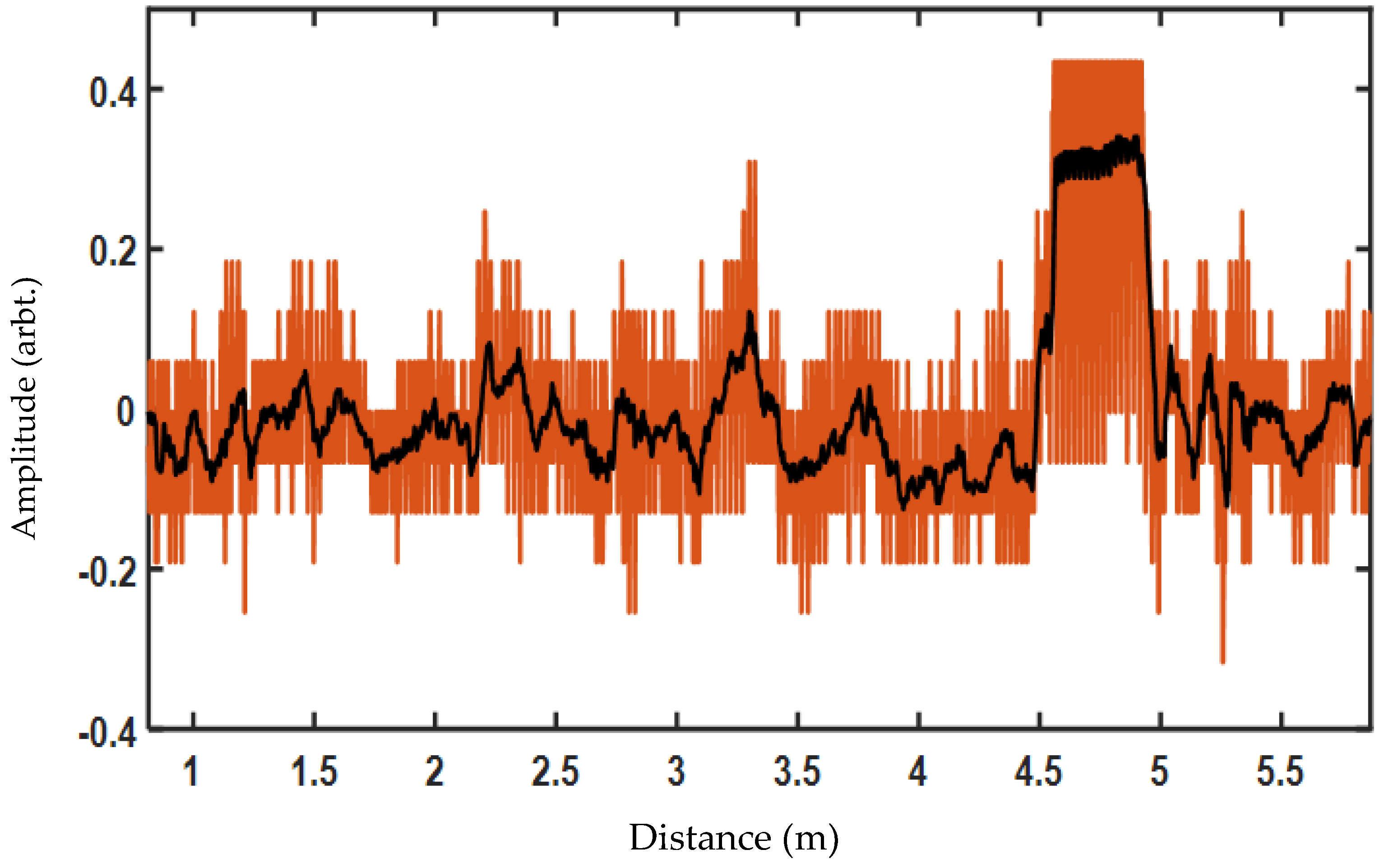
Figure 6 shows the Teletest signal of Test 5 before processing, where the defect’s signal region is in between the two dotted red lines. The SNR of a defect in this test is −0.98 dB, which means that it is completely buried in the noise. The noise signal is calculated by removing the torsional waves (pipe end and defect signal) from the shown signal in Figure 6. However, since Defect 2 is not present in this test, the location in between 4–4.5 m is also considered as noise.
Figure 7 shows the assigned values to the first (black line) and the second version (red line) of thresholding, which is the and subtraction of the from the , respectively. As can be seen both in the backward leakage signal and the noise region, the decrease in the assigned threshold is more than the defect and pipe end signals. In method two, a static percentage of either of the mentioned values is considered the threshold for each iteration; however, in method three, this percentage is assigned using the ratios of signals subtracted from its mean, as shown in Figure 8. The calculated threshold for each iteration using the average value of method three is shown in Figure 9. In the same figure, if method one was used, the threshold value would be a constant line for all of the iterations. The processed signal calculated from method three is illustrated in Figure 10, where it shows the locations at which the is higher than the threshold history. As expected, the pipe end is completely detected, since it is a complete axisymmetric feature, but only the center part of the defect could be detected.
5.2. First Set of Tests
The detection of Defect 1 is the focus in the first set of tests (test numbers 1–6). In these test cases, Defect 2 does not exist, and therefore, the region between 4–4.5 is considered noise. Furthermore, the coherent flexural noises existing in the Defect-1 region are less than those in the second Defect-2 region, with 34 kHz, 30 kHz, and 37 kHz having the least amounts, respectively. As can be seen from Table 3, the defects in these tests have a low SNR and are almost buried in temporal noise, which makes them difficult to be detected in the temporal domain.
5.2.1. Method One
This method was only successful for tests 1, 2, and 4. Figure 11 shows the limits of the threshold values. Observing the trends with regards to the frequency in tests 1–3, the minimum values are increasing, while the maximum values are decreasing up until the point where the minimum will result in an outlier in Test 3. The same trend is observable for the minimum values in tests 4–6, where, although the maximum values could not be detected, the minimum values are increasing with regard to the frequency. With regard to the defect CSA (and SNR), the algorithm can detect the 2% CSA defect using a 30-kHz excitation frequency (Test 4). Nonetheless, when the frequency is increased to 34 kHz in Test 5, although the defect’s SNR is increased by 1.68 dB, this method resulted in a false alarm, even at the minimum limit. Thus, it can be concluded that this algorithm is more sensitive to the frequency and local amplitude of the defect region rather than its temporal SNR and the overall energy of the noises in the region. Since higher energy is associated with lower frequencies, lower frequencies tests would achieve better results using this method for Defect 1.
5.2.2. Method Two
This method is effective in all of the tests except for Test 6. With regard to Figure 12, which shows the limits achieved using this method, the relation between the detection limits and frequency is no longer linear. The minimum is increasing with the frequency until it reaches a maximum peak on 34 kHz; then, it starts to decrease when moving toward 37 kHz. The same trend is observable for the detection length and safe zone margins. This means that this algorithm is a function of both the SNR of the noise and the defect, as well as the frequency where the optimum frequency would be around 34 kHz. Nonetheless, it should also be pointed out that when using a lower frequency, the same happens as in the previous method: the minimum value for detection is closer to zero, which means that defects would be easier to detect. Regarding the second thresholding version, the increase in the minimum limits is not as much as those in the maximum, which therefore increases the safe zone margins in all of the tests. This is clearly observable in tests 1 and 2, where the minimum limits remained unchanged. The average and maximum detection lengths of the defect remain unchanged. Therefore, using the second threshold version provides a greater safe zone margin.
In comparison to method one, this method has a greater range of operating frequencies and provides a larger safety margin for threshold selection. The optimum excitation frequency for this method is 34 kHz for the first set of tests.
5.2.3. Method Three
The average values are calculated automatically by taking the mean of the percentage of active sensors in each iteration; thus, they are fixed in both thresholding versions. The same as method two, this method can detect the defects without any false alarms in tests 1–5. However, only tests with an excitation frequency of 34 kHz can use the average value, since using it for other excitation frequencies would result in detecting outliers. The limits of this method are shown in Figure 13. The tests where the average value is between the minimum and maximum are when the automatic detection method is successful. Furthermore, the averages values achieved using all of the different frequencies are between 0.602–0.554, and tend to decrease slightly when the frequency is increased.
To conclude, this method can automatically detect defects of up to 2% CSA, which are buried in the noise level using a 34-kHz excitation frequency. Furthermore, with regard to the detection length, it can also be said that 34 kHz is the optimum excitation frequency in the first set of tests.
5.2.4. Comparison
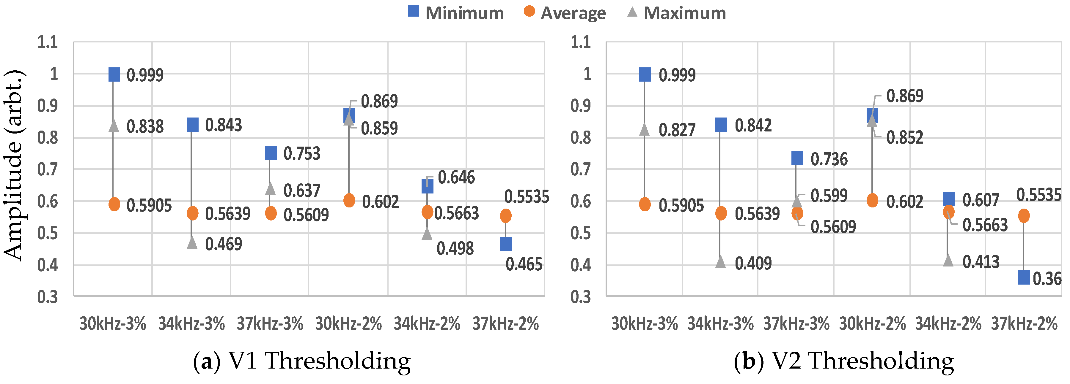
Figure 14 shows the amount of increase in the minimum and maximum values achieved using the first and second version of the thresholding. The minimums tend to increase less than the maximum values by at least a factor of two.
The generated safe zone margins for all of the methods are shown in Figure 15. Except for Test 4, method three tends to have a higher safe zone margin than method two, and the best margin is achieved using second thresholding version for method three. These results are especially important on tests 2 and 5, where the optimum excitation frequency of both methods is used. The second version of thresholding always produces a greater safety margin.
Figure 16 shows the length of detection achieved by average values with different algorithms. Cases where outliers are detected are not reported. As can be seen, in the optimum frequency, both of the defect lengths achieved by method two and method three are the same. In Test 5, in the second version of thresholding, the length has decreased, since the average value is fixed, and the defect size is smaller; however, in Test 2, the same detection length is achieved using both versions, since the defect is wider. Method three is the best out of these three mentioned ones, since it produces a larger safe zone margin, and can detect the defects automatically using the optimum excitation frequency of 34 kHz for the first set of tests.
5.3. Second Set of Tests
In the second set of trials, the focus is on detecting Defect 2. The defect signal is expected to be received between 4–4.5 m. Since the baseline of the defect signal is highly polluted by the coherent flexural noise, higher detection limits are required for detecting the defects, even when the CSA size of the defect is increased. This aim of these tests is to observe the effect of spatial noise on the algorithm and demonstrate its capability in detecting defects in such scenarios. Since excitation frequencies of 37 kHz, 34 kHz, and 30 kHz have the lowest spatial noise in the defect region, respectively, it is expected that the algorithms perform better using the respective mentioned frequencies.
5.3.1. Method One
Figure 17 shows the limits required from method one to detect Defect 2. The only excitation frequency that allowed the detection of defects without any outliers was 37 kHz, while 34 kHz resulted in the detection of defects with at least three outliers in both cases, and in 30 kHz, the defect could not be detected. With 37 kHz as the excitation frequency, it can be seen that when the defect energy decreases, the threshold is increased to 0.009. As this value is close to the maximum allowable threshold (0.01), no smaller defects could be detected even using this frequency. This is unlike the first set of tests, where it was easier to detect the defect using lower frequencies, since Defect 2 is located in a region with higher energies of flexural noises. Consider the case of the 34-kHz frequency, as reported in Figure 11: the maximum limit of detection of Defect 1 without any outliers is approximately 0.013. However, in the case of Defect 2, the minimum level is 0.019 for the 5% CSA defect, which is higher than the previously reported limit. This outcome indicates the detection of outliers in the test. The same can also be said regarding 37 kHz, where previously, the maximum limit was approximately 0.012, and now, the minimum required for the detection of a 4% CSA defect is 0.01, which is below the level where outliers will be detected. It can be concluded that method one is highly affected by the existing energy of flexurals in the same iteration.
5.3.2. Method Two
The results of method two are illustrated in Figure 18. Unlike the first set of tests, where 34 kHz was the optimum frequency of excitation, in these tests, 37 kHz achieves better results. It is not possible to detect Defect 2 without any outliers using the 30-kHz frequency, since the required minimum threshold level, 0.125, is higher than the maximums that are reported in Figure 13. Nonetheless, using the two other frequencies, Defect 2 can be detected. From the margins, it is evident that 37 kHz achieves the highest safe zone margin required for detection, where both the minimum and maximum thresholds that are required are respectively lower and higher than the ones required for other frequencies. Furthermore, when the defect size decreases, the limits are not affected significantly, which suggests that when using 37 kHz, smaller defect sizes than 4% CSA can be detected. In fact, in this region, defects with CSAs as small as 2% can only be detected using this frequency using both method two and method three.
Compared to method one, although the limits have been increased in the case of Defect 2, it can be seen that it is not affected as much, since method two is capable of detecting defects using 34 kHz without any outliers and 30 kHz with outliers. Nonetheless, this method also performs best in the absence of flexurals in the same location as the defect signal.
5.3.3. Method Three
Figure 19 shows the results achieved using method three. These are the same as before in the tests where the average detection values are in between the minimum and maximum thresholds; namely, the tests using 37 kHz as the excitation frequency are the tests where the defects can be automatically detected without any outliers when using this method. Same as the other methods, using 30 kHz for detection of Defect 2 is only possible when outliers are also reported. For the case of 34 kHz, when using the average value, it is not possible to detect Defect 2 without any outliers. However, it can be seen when using the second version of the thresholding value that the minimum detection value is significantly closer to the average value, which clearly illustrates the advantage of this version.
5.3.4. Comparison
Figure 20 shows the number of increments observed in the limits when V2 is used. It is the same as in the first test case: the minimums tend to increase less than the maximums. In tests using 30 kHz, since outliers are detected, the same amount of increment is reported.
The generated safe zone margins for the second set of tests are demonstrated in Figure 21. As expected, V2 always provides a greater safe zone margin. This is especially important in the case of method three, since generally, the minimums that are required for detection are well above the average value, while the maximums are close. The benefit of using V2 is clearly illustrated in Figure 19, where upon testing with the 34-kHz frequency, the maximum detection value of V2 in both tests is much closer to the calculated average value.
The average detection lengths achieved using all of the methods are shown in Figure 22 using the optimum frequency (37 kHz) for detecting Defect 2. Both methods two and three achieve the same detection length for 5% CSA; nonetheless, when the defect size decreases, method three tends to have a higher detection length. In the tests with a 34-kHz excitation frequency, method two achieved a higher detection length, since the average value is not set mathematically. Using the optimum frequency, it can be concluded that method three is the best method, since it generated the most detection length with the highest safe zone margin.
6. Conclusions
In this paper, a novel statistical algorithm was proposed that uses the full capability of the tool-set array of conventional guided waves inspection devices to identify defect signals that have been polluted by coherent noise. Laboratory trials confirmed the effectiveness of this algorithm in detecting defects with low/negative SNRs and its dependence on the frequency.
Three different methods and two different versions were created for generating the results, in which the thresholding scheme of each was different. In method one, the threshold is a static value set by the inspector. In method two, the assigned threshold to each iteration is a percentage taken from the summation of the amplitude of all of the transducers signals with the same as the time-domain signal generated by the normal propagation routine. In method three, the percentage value is determined by determining the number of transducers with the same phase over the total number of transducers, subtracted by an offset. Two versions of method two and method three are also developed, wherein the second version, the summation of signals with the same sign as the temporal signal was subtracted from the comparisonValue, before determining the final assigned threshold of each iteration. The following conclusions can be drawn with regards to the tests done:
- Method Comparison: Method one tended to produce the worst results, as it solely depended on a static value set by the user without considering the characteristics of the signals received in each iteration. Methods two and three can achieve a similar result in most cases; however, in method three, the threshold value can be set automatically, which provides a great benefit in one-off inspection scenarios.
- Version Comparison: Version 2 always produced a wider safe zone margin while achieving approximately the same defect detection length using the average values.
- Excitation Frequency: In the first set of tests, by lowering the frequency, a greater safe zone margin and a lower threshold value is required for method one. However, in the second set of tests, the exact opposite occurs. Therefore, method one is highly affected by the regional flexural waves, and high torsional energies are required for detection. However, both of the other methods have an optimum excitation frequency of 34 kHz for the first set of tests, and 37 kHz for the second set of tests. This suggests that all of the methods are more affected by the existing spatial noises caused by the flexural waves in the same iteration rather than the temporal noise of the neighborhood. The second set of tests also clearly illustrates the advantages of method two and method three in detecting defects in locations where a higher level of coherent noise exists.
- Safe Margin Zones: Method three (V2) always achieved the highest safe zone margin, and is therefore the safest method to use.
- With regard to these results, method three (V2) is the best method since the threshold can be determined automatically, and it achieves the highest safe zone margin. The tests prove that this method can detect defects using both 34 kHz and 37 kHz, depending on the existing coherent noise in the defect location. Furthermore, the algorithm is sensitive to the existing coherent noises in the baseline signal rather than the temporal noise in the tests.
This newly developed algorithm can be used to help the inspectors as an additional tool, allowing them an easier interpretation of the results. This is the main reason why all of the developed methods are mentioned. It also enables the possibility of developing narrowband transducers, as opposed to the currently used wideband transducers, which have a more focused transfer function and stronger excitation power.
In this paper, we have defined a new pathway for solving the problem of defect identification in the UGW inspection of pipelines. In this pathway, we use the information of both space and time to automatically detect defect signals rather than trying to minimize the coherent noise by spatial averaging techniques and interpreting the results based on their properties in a time domain. Thus, the main message of this paper was to illustrate the effectiveness of such approaches, which are feasibly applicable to the current systems of guided-wave testing.
Author Contributions
Conceptualization, H.N.M.; Data curation, H.N.M.; Formal analysis, H.N.M.; Funding acquisition, H.N.M.; Investigation, H.N.M.; Methodology, H.N.M.; Project administration, H.N.M.; Resources, H.N.M.; Software, H.N.M.; Supervision, H.N.M., K.Y. and A.K.N.; Validation, H.N.M.; Visualization, H.N.M., K.Y. and A.K.N.; Writing—original draft, H.N.M.; Writing—review & editing, H.N.M. and A.K.N.
Funding
This research study was made possible by the sponsorship and support of Brunel University London and National Structural Integrity Research Centre (NSIRC).
Conflicts of Interest
The authors declare no conflicts of interest.
References
- Ostachowicz, W.M. Guided Waves in Structures for SHM: The Time-Domain Spectral Element Method; Wiley: Hoboken, New Jersey, NJ, USA, 2012. [Google Scholar]
- Lowe, M.J.S.; Cawley, P. Long Range Guided Wave Inspection Usage—Current Commercial Capabilities and Research Directions; Imperial College: London, 2016; Available online: http://www3.imperial.ac.uk/pls/portallive/docs/1/55745699.PDF (accessed on 19 October 2018).
- Lowe, M.J.S.; Alleyne, D.N.; Cawley, P. Defect detection in pipes using guided waves. Ultrasonics 1998, 36, 147–154. [Google Scholar] [CrossRef]
- Thornicroft, K. Ultrasonic Guided Wave Testing of Pipelines using a Broadband Excitation; Brunel University London: London, UK, 2015. [Google Scholar]
- Pavlakovic, B. Signal Processing Arrangment. U.S. Patent 2006/0203086 A1. 14 September 2006. [Google Scholar]
- ASTM Standard E2775–16. Standard Practice for Guided Wave Testing of above Ground Steel Pipeword Using Piezoelectric Effect Transduce; ASTM International: West Conshohocken, PA, USA, 2017. [Google Scholar]
- Wilcox, P.D. A rapid signal processing technique to remove the effect of dispersion from guided wave signals. IEEE Trans. Ultrason. Ferroelectr. Freq. Control 2003, 50, 419–427. [Google Scholar] [CrossRef] [PubMed]
- Zeng, L.; Lin, J.; Lei, Y.; Xie, H. Waveform design for high-resolution damage detection using lamb waves. IEEE Trans. Ultrason. Ferroelectr. Freq. Control 2013, 60, 1025–1029. [Google Scholar] [CrossRef] [PubMed]
- Yücel, M.K.; Fateri, S.; Legg, M.; Wilkinson, A.; Kappatos, V.; Selcuk, C.; Gan, T.H. Coded Waveform Excitation for High-Resolution Ultrasonic Guided Wave Response. IEEE Trans. Ind. Inform. 2016, 12, 257–266. [Google Scholar] [CrossRef]
- Yücel, M.K.; Fateri, S.; Legg, M.; Wilkinson, A.; Kappatos, V.; Selcuk, C.; Gan, T.H. Pulse-compression based iterative time-of-flight extraction of dispersed Ultrasonic Guided Waves. In Proceedings of the 2015 IEEE 13th International Conference on Industrial Informatics (INDIN), Cambridge, UK, 22–24 July 2015; pp. 809–815. [Google Scholar]
- Lin, J.; Hua, J.; Zeng, L.; Luo, Z. Excitation Waveform Design for Lamb Wave Pulse Compression. IEEE Trans. Ultrason. Ferroelectr. Freq. Control 2016, 63, 165–177. [Google Scholar] [CrossRef] [PubMed]
- Malo, S.; Fateri, S.; Livadas, M.; Mares, C.; Gan, T. Wave Mode Discrimination of Coded Ultrasonic Guided Waves using Two-Dimensional Compressed Pulse Analysis. IEEE Trans. Ultrason. Ferroelectr. Freq. Control 2017, 64, 1–10. [Google Scholar] [CrossRef] [PubMed]
- Song, X.; Ta, D.; Wang, W. A base-sequence-modulated golay code improves the excitation and measurement of ultrasonic guided waves in long bones. IEEE Trans. Ultrason. Ferroelectr. Freq. Control 2012, 59, 2580–2583. [Google Scholar] [PubMed]
- Pedram, S.K.; Haig, A.; Lowe, P.S.; Thornicroft, K.; Gan, L.; Mudge, P. Split-spectrum signal processing for reduction of the effect of dispersive wave modes in long-range ultrasonic testing. Phys. Procedia 2015, 70, 388–392. [Google Scholar] [CrossRef]
- Pedram, S.K.; Fateri, S.; Gan, L.; Haig, A.; Thornicroft, K. Split-spectrum processing technique for SNR enhancement of ultrasonic guided wave. Ultrasonics 2018, 83, 48–59. [Google Scholar] [CrossRef] [PubMed]
- Fateri, S.; Boulgouris, N.V.; Wilkinson, A.; Balachandran, W.; Gan, T.H. Frequency-sweep examination for wave mode identification in multimodal ultrasonic guided wave signal. IEEE Trans. Ultrason. Ferroelectr. Freq. Control 2014, 61, 1515–1524. [Google Scholar] [CrossRef] [PubMed]
- Ng, C.-T. On the selection of advanced signal processing techniques for guided wave damage identification using a statistical approach. Eng. Struct. 2014, 67, 50–60. [Google Scholar] [CrossRef] [Green Version]
- Clarke, T.; Simonetti, F.; Cawley, P. Guided wave health monitoring of complex structures by sparse array systems: Influence of temperature changes on performance. J. Sound Vib. 2010, 329, 2306–2322. [Google Scholar] [CrossRef]
- Lu, Y.; Michaels, J.E. A methodology for structural health monitoring with diffuse ultrasonic waves in the presence of temperature variations. Ultrasonics 2005, 43, 717–731. [Google Scholar] [CrossRef] [PubMed]
- Chang, Y.; Zi, Y.; Zhao, J.; Yang, Z.; He, W.; Sun, H. An adaptive sparse deconvolution method for distinguishing the overlapping echoes of ultrasonic guided waves for pipeline crack inspection. Meas. Sci. Technol. 2017, 28, 035002. [Google Scholar] [CrossRef] [Green Version]
- Davies, J.; Cawley, P. The application of synthetic focusing for imaging crack-like defects in pipelines using guided waves. IEEE Trans. Ultrason. Ferroelectr. Freq. Control 2009, 56, 759–770. [Google Scholar] [CrossRef] [PubMed]
- Roberts, A.; Pardini, R.; Diaz, A. High frequency guided wave virtual array SAFT. Rev. Quant. Nondestruct. Eval. 2003, 22, 205–212. [Google Scholar]
- Luo, W.; Rose, J.L.; van Velsor, J.K.; Mu, J. Phased-array focusing with longitudinal guided waves in a viscoelastic coated hollow cylinder. AIP Conf. Proc. 2006, 820, 869–876. [Google Scholar]
- Davies, J. Inspection of Pipes Using Low Frequency Focused Guided Waves; Imperial College London: London, UK, 2008. [Google Scholar]
- Davies, J.; Simonetti, F.; Lowe, M.; Cawley, P. Review of Synthetically Focussed Guided Wave Imaging Techniques with Application to Defect Sizing. In Proceedings of the European Conference on Nondestructive Testing 2006, Berlin, Germany, 25 September 2006; pp. 1–9. [Google Scholar]
- Sicard, R.; Chahbaz, A.; Goyette, J. Guided lamb waves and L-SAFT processing technique for enhanced detection and imaging of corrosion defects in plates with small depth-to-wavelength ratio. IEEE Trans. Ultrason. Ferroelectr. Freq. Control 2004, 51, 1287–1297. [Google Scholar] [CrossRef] [PubMed]
- Fu, H.; Wu, B.; He, C.; Wang, W. A synthetic digital signal processing method of ultrasonic guided wave pipeline inspection. In Proceedings of the International Conference on Image Analysis and Signal Processing, Hubei, China, 21–23 October 2011; pp. 444–446. [Google Scholar]
- Meitzler, A.H. Mode Coupling Occurring in the Propagation of Elastic Pulses in Wires. J. Acoust. Soc. Am. 1961, 33, 435–445. [Google Scholar] [CrossRef]
- Rose, J.L. Ultrasonic Guided Waves in Solid Media; Cambridge University Press: Cambridge, UK, 2014. [Google Scholar]
- Mahal, H.N.; Mudge, P.; Nandi, A.K. Comparison of coded excitations in the presence of variable transducer transfer functions in ultrasonic guided wave testing of pipelines. In Proceedings of the 9th European Workshop on Structural Health Monitoring, Manchester, UK, 10–13 July 2018. [Google Scholar]
- Lowe, M.J.S.; Alleyne, D.N.; Cawley, P. The Mode Conversion of a Guided Wave by a Part- Circumferential Notch in a Pipe. J. Appl. Mech. 1998, 65, 649–656. [Google Scholar] [CrossRef]
- Nurmalia. Mode Conversion of Torsional Guided Waves for Pipe Inspection: An Electromagnetic Acoustic Transducer Technique; Osaka University: Osaka, Japan, 2013. [Google Scholar]
- Teletestndt, Long Range Guided Wave Testing with Teletest Focus+. 2018. Available online: https://www.teletestndt.com/ (accessed on 19 October 2018).
Figure 1.
Spatial signal reception from two rings of 32 source points from various features where the red, blue, and black dotted lines are showing the first ring, second ring, and the reference offset.
Figure 1.
Spatial signal reception from two rings of 32 source points from various features where the red, blue, and black dotted lines are showing the first ring, second ring, and the reference offset.

Figure 2.
Temporal domain of cases (d)–(i) from Figure 1
Figure 2.
Temporal domain of cases (d)–(i) from Figure 1

Figure 3.
System flowchart.

Figure 4.
Signal reception routes.

Figure 5.
Baseline signals of pipe with no defect with frequencies of (a) 30 kHz; (b) 34 kHz; and (c) 37 kHz. The first marked region (3–3.5 m) is the location of the first defect, and the second marked region (4.1–4.5) is the location of the second defect.
Figure 5.
Baseline signals of pipe with no defect with frequencies of (a) 30 kHz; (b) 34 kHz; and (c) 37 kHz. The first marked region (3–3.5 m) is the location of the first defect, and the second marked region (4.1–4.5) is the location of the second defect.

Figure 6.
Example signal achieved using general routine, tested by 34 kHz where the first two red dotted lines shows the defect region, and the third and fourth ones show the pipe end.
Figure 6.
Example signal achieved using general routine, tested by 34 kHz where the first two red dotted lines shows the defect region, and the third and fourth ones show the pipe end.

Figure 7.
Comparison of the first and second thresholding versions on the Test 5 signal where the two zoomed regions are showing the backward leakage, defect, noise, and pipe end, respectively. The black and red signals are showing the first and second versions, respectively.
Figure 7.
Comparison of the first and second thresholding versions on the Test 5 signal where the two zoomed regions are showing the backward leakage, defect, noise, and pipe end, respectively. The black and red signals are showing the first and second versions, respectively.

Figure 8.
Calculated percentage of sensors with same phase, where the offset (mean values) are removed (orange); the black signal is showing the filtered version for better illustration.
Figure 8.
Calculated percentage of sensors with same phase, where the offset (mean values) are removed (orange); the black signal is showing the filtered version for better illustration.

Figure 9.
Calculated threshold using method three on Test 5 (red) against the second version comparisonValue (black). In the case of method one, the threshold would be a constant line instead of changing based on the iteration.
Figure 9.
Calculated threshold using method three on Test 5 (red) against the second version comparisonValue (black). In the case of method one, the threshold would be a constant line instead of changing based on the iteration.

Figure 10.
Method three result (green signal) using the average value against the temporal signal (black) for testing a 2% CSA defect.
Figure 10.
Method three result (green signal) using the average value against the temporal signal (black) for testing a 2% CSA defect.

Figure 11.
Minimum, average, and maximum values of method one of the first set of tests.

Figure 12.
Limits achieved using method two on the first set of tests.

Figure 13.
Limits achieved using method three in the first set of tests.

Figure 14.
The increments achieved using the second version of thresholding in the first set of tests.
Figure 14.
The increments achieved using the second version of thresholding in the first set of tests.

Figure 15.
Bar graphs of the Safe zone margins of all methods in the first set of tests.

Figure 16.
Bar graphs of the detection length of the defect using the average value of all of the methods in the first set of tests.
Figure 16.
Bar graphs of the detection length of the defect using the average value of all of the methods in the first set of tests.

Figure 17.
Minimum, average, and maximum values of method one of the second test cases.

Figure 18.
Limits achieved using method two on the second set of tests.

Figure 19.
Limits achieved using method three on the second set of tests.

Figure 20.
The increments achieved using the second version of thresholding in the second set of tests.
Figure 20.
The increments achieved using the second version of thresholding in the second set of tests.

Figure 21.
Bar graphs of the Safe zone margins of all methods in the second set of tests.

Figure 22.
Bar graphs of detection length of the defect using the average value of all of the methods in the second set of tests.
Figure 22.
Bar graphs of detection length of the defect using the average value of all of the methods in the second set of tests.


Table 1.
Summary of the first set of tests conditions (first defect). CSA: cross-sectional area.
| Test (#) | Defect CSA (%) | Frequency (kHz) |
|---|---|---|
| 1 | 3 | 30 |
| 2 | 34 | |
| 3 | 37 | |
| 4 | 2 | 30 |
| 5 | 34 | |
| 6 | 37 |
Table 2.
Summary of the second set of tests conditions (second defect).
| Test (#) | Defect CSA (%) | Frequency (kHz) |
|---|---|---|
| 7 | 5 | 30 |
| 8 | 34 | |
| 9 | 37 | |
| 10 | 4 | 30 |
| 11 | 34 | |
| 12 | 37 |
Table 3.
Calculated signal-to-noise ratio (SNR) with respect to the coherent noises in the inspection (in dB).
Table 3.
Calculated signal-to-noise ratio (SNR) with respect to the coherent noises in the inspection (in dB).
| Test # | 1 | 2 | 3 | 4 | 5 | 6 | 7 | 8 | 9 | 10 | 11 | 12 |
|---|---|---|---|---|---|---|---|---|---|---|---|---|
| SNR | 2.97 | 8.93 | 10.36 | −2.65 | −0.98 | −3.43 | 18.57 | 27.63 | 28.05 | 14.73 | 24.00 | 23.10 |
© 2018 by the authors. Licensee MDPI, Basel, Switzerland. This article is an open access article distributed under the terms and conditions of the Creative Commons Attribution (CC BY) license (http://creativecommons.org/licenses/by/4.0/).
Share and Cite
MDPI and ACS Style
Mahal, H.N.; Yang, K.; Nandi, A.K. Detection of Defects Using Spatial Variances of Guided-Wave Modes in Testing of Pipes. Appl. Sci. 2018, 8, 2378. https://doi.org/10.3390/app8122378
AMA Style
Mahal HN, Yang K, Nandi AK. Detection of Defects Using Spatial Variances of Guided-Wave Modes in Testing of Pipes. Applied Sciences. 2018; 8(12):2378. https://doi.org/10.3390/app8122378
Chicago/Turabian StyleMahal, Houman Nakhli, Kai Yang, and Asoke K. Nandi. 2018. "Detection of Defects Using Spatial Variances of Guided-Wave Modes in Testing of Pipes" Applied Sciences 8, no. 12: 2378. https://doi.org/10.3390/app8122378
Note that from the first issue of 2016, this journal uses article numbers instead of page numbers. See further details here.