Time-Domain Hydro-Elastic Analysis of a SFT (Submerged Floating Tunnel) with Mooring Lines under Extreme Wave and Seismic Excitations


Department of Ocean Engineering, Texas A&M University, Haynes Engineering Building, 727 Ross Street, College Station, TX 77843, USA
*
Author to whom correspondence should be addressed.
Appl. Sci. 2018, 8(12), 2386; https://doi.org/10.3390/app8122386
Submission received: 19 October 2018
/
Revised: 19 November 2018
/
Accepted: 22 November 2018
/
Published: 26 November 2018
(This article belongs to the Special Issue Modelling, Simulation and Data Analysis in Acoustical Problems)
Abstract
:Global dynamic analysis of a 700-m-long SFT section considered in the South Sea of Korea is carried out for survival random wave and seismic excitations. To solve the tunnel-mooring coupled hydro-elastic responses, in-house time-domain-simulation computer program is developed. The hydro-elastic equation of motion for the tunnel and mooring is based on rod-theory-based finite element formulation with Galerkin method with fully coupled full matrix. The dummy-connection-mass method is devised to conveniently connect objects and mooring lines with linear and rotational springs. Hydrodynamic forces on a submerged floating tunnel (SFT) are evaluated by the modified Morison equation for a moving object so that the hydrodynamic forces by wave or seismic excitations can be computed at its instantaneous positions at every time step. In the case of seabed earthquake, both the dynamic effect transferred through mooring lines and the seawater-fluctuation-induced seaquake effect are considered. For validation purposes, the hydro-elastic analysis results by the developed numerical simulation code is compared with those by a commercial program, OrcaFlex, which shows excellent agreement between them. For the given design condition, extreme storm waves cause higher hydro-elastic responses and mooring tensions than those of the severe seismic case.
1. Introduction
The submerged floating tunnel (SFT) is an innovative solution used to cross deep waterways [1,2]. The SFT consists mainly of a tunnel for vehicle transportation and mooring lines for station-keeping. The tunnel is usually positioned at a certain submergence depth, typically greater than 20 m, with positive net buoyancy that is balanced by mooring lines anchored in the seabed [3,4].
Considering that wave/current/wind effects are greatly reduced, the cost is almost constant along the length [5], and ship passage is not obstructed by the structure, the SFT has been regarded as a competitive alternative to floating bridges and immersed tunnels. In this regard, since Norway’s first patent in 1923 [6], many proposals and case studies have been published worldwide, which includes Høgsfjord/Bjørnafjord in Norway [7,8,9], the Strait of Messina in Italy [10], Funka Bay in Japan [11,12], Qiandao Lake in China [13,14], and the Mokpo-Jeju SFT in Korea [15]. Even though there is no actually installed structure in the world despite extensive research [16], the first construction of the SFT is being considered by Norwegian Public Road Administration (NPRA) with global interest [17].
To provide sufficient confidence for the concept, feasibility studies under diverse catastrophic environmental conditions, such as extreme waves and earthquakes, must be extensively studied in advance. Along this line, numerous researches have been carried out to verify structural safety in wave and seismic excitations on the SFT. Regarding wave-excitation effects, Kunisu et al. [18] evaluated the effect of mooring-line configurations on SFT dynamic responses including possible snap loading. Lu et al. [11] and Hong et al. [19] focused on slack mooring phenomena at various buoyancy-weight ratios (BWRs) of the SFT and inclination angles of mooring lines. Long et al. [3] conducted parametric studies to investigate the effects of the BWR and mooring-line stiffness. Dynamic motions at varying BWRs and the corresponding comfort index were investigated by Long et al. [20]. Seo et al. [21] compared experimental results with simplified numerical approach for a segment of the SFT. Chen et al. [22] evaluated the influence of VIV (vortex induced vibration) of mooring lines on the SFT dynamic responses using a simplified numerical model. In addition, with regard to seismic-excitation effects, Di Pilato et al. [4] carried out a coupled dynamic analysis to investigate the effect of wave and seismic excitations. Martinelli et al. [13] suggested detailed procedures to generate artificial seismic excitations and performed the corresponding structural analysis. Dynamic responses at various shore connections under transverse earthquake were investigated by Xiao and Huang [23]. Martinelli et al. [24] and Wu et al. [25] focused on hydrodynamic fluid-structure interaction induced by vertical fluid fluctuations known as the seaquake. Mirzapour et al. [26] derived simplified analytical solutions for 2D and 3D cases and computed SFT dynamic responses in diverse stiffness conditions. Muhammad et al. [6] compared the dynamic effects induced by wave and seismic excitations.
During the past decade, various SFT-related studies have been carried out in the second author’s research lab. Cifuentes et al. [27] compared the dynamics of a moored-SFT segment in regular waves for various BWRs and mooring types between experimental results and numerical simulations. For the numerical simulations, both commercial program (OrcaFlex) and in-house program CHARM3D (Coupled Hull And Riser Mooring 3D) were used for cross-checking. Lee et al. [16] further investigated the dynamics of the short tunnel segment under irregular waves and random seabed earthquakes. Then, the initial studies of hydro-elastic responses of a long SFT with many mooring lines by random waves and seabed earthquakes were conducted by Jin and Kim [28] and Jin et al. [29] by using commercial software, OrcaFlex. However, when using OrcaFlex for seismic excitations, an indirect modeling with many seabed dummy masses has to be introduced instead of direct inputs of dynamic boundary conditions at those anchor points.
In this research, to add the capability of hydro-elastic analyses of a long SFT with many mooring lines in the in-house coupled dynamic-analysis program, a new approach called ‘dummy-connection-mass method’ is developed. The equation of motion for the line element is derived by rod theory, and finite element modelling is implemented by using Galerkin method. Linear and rotational springs are employed to conveniently connect several objects with given connection conditions. The Adams–Moulton implicit integration method combined with the Adam–Bashforth explicit scheme, is used for the time-domain-integration method so that stable and time-efficient numerical integration can be done without iteration. The newly developed program is applied to calculate the hydro-elastic responses of a 700-m-long SFT (with both ends fixed) with many mooring lines by extreme random waves or severe random earthquakes. The results from the newly developed program are cross-checked against those from OrcaFlex program. In the case of seabed earthquake, the seabed motions are transferred to the SFT through mooring lines and through seawater fluctuations called seaquake, which is extensively discussed in Section 4 based on the produced numerical results. In the present study, the effect of seismic-induced acoustic pressure is not considered since the resulting frequency range is much higher [30], and thus it is of little importance for the mooring design.
2. Configuration of the System
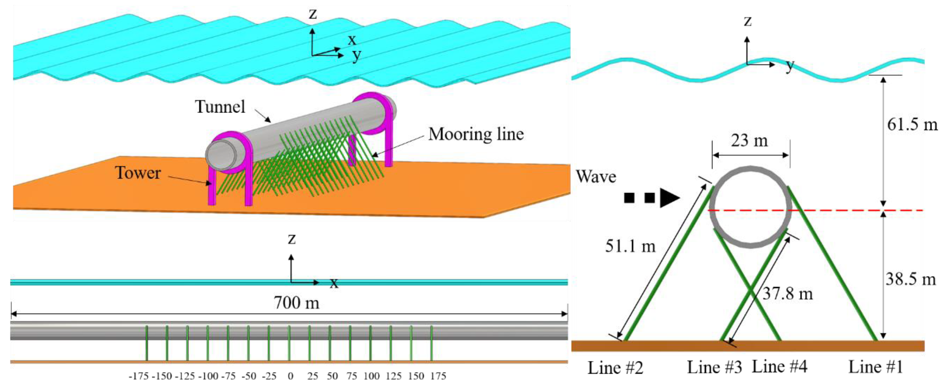
Figure 1 shows 2D and 3D views of the entire structure, and Table 1 summarizes major design parameters of the tunnel and mooring lines. The tunnel, which has a diameter of 23 m and a length of 700 m, is made of high-density concrete. Since the structure in this study is a section of the 30-km-long SFT, the fixed-fixed boundary condition at both ends are applied assuming that strong fixtures (or towers) will be built at 700-m intervals, as shown in the Figure 1. Considering that the water depth of the planned site is 100 m, the submergence depth, a vertical distance between free surface and the tunnel centerline, is set to be 61.5 m. The BWR is fixed at 1.3, and the tunnel thickness is 2.3 m. The tunnel thickness is actually greater than the real value to have the equivalent tunnel bending stiffness including inner compartment structures. The axial and bending stiffnesses are calculated based on the given data of Table 1.
Chain mooring lines with a nominal diameter of 180 mm are used. High static and dynamic mooring tensions are expected based on the given BWR and wave condition [28]. In addition, the maximum mooring tension should be smaller than the MBL (minimum breaking load) divided by safety factor (SF). Thus, chain might be the best choice considering high MBL of 30,689 kN for Grade R5. As shown in Figure 1, four 60-degree-inclined mooring lines are installed for every 25 m interval toward the center locations. The lengths of mooring lines are 51.1 m for line #1 and #2 and 37.8 m for line #3 and #4. The wet natural frequencies of the tunnel hydro-elastic responses coupled with mooring lines are calculated and presented in Table 2.
3. Numerical Model
Tunnel-mooring coupled dynamic analysis was conducted by using the in-house program, CHARM3D. This in-house code has been developed by second author’s research lab for the coupled dynamic simulations of complex offshore structures with mooring lines and risers during the past two decades [34,35]. In addition, the capability has further been expanded for various applications including multiple bodies connected by lines, wind turbines [36], dynamic positioning [37], and ice-structure interactions [38]. The program is further extended in this paper to study the SFT hydro-elastic dynamics for seismic excitations. In addition, some of the computed results are compared with those by widely-used commercial program OrcaFlex for cross-checking. In the following equations, bold variables represent vectors or matrices.
3.1. Governing Equations of Dynamic Simulation
The entire structure is modelled by rod elements and the rod theory suggested by Garrett [39] is used. The behavior of the rod element is determined by the position of the rod centerline. The equation of motion is solved in general coordinate whose tangential direction follows the line profile; therefore, coordinate transformations, which increase computation time, are not required. In addition, geometric non-linearity is considered without specific assumptions associated with the shape or orientation of lines [34]. The equation of motion and the extensible condition are presented in Equations (1) and (2).
where is a position vector, which is a function of arc length and time in order to define space curve, is Young’s modulus, is second moment of sectional area, is Lagrange multiplier, and are the distributed load and mass per unit length, is the tension, and is the cross sectional area filled with the material. In addition, dot and apostrophe denote time and spatial derivatives, respectively. The distributed load includes the weight of the rod and hydrostatic and hydrodynamic loads induced by the surrounding fluid. The hydrostatic load is subdivided into buoyancy and force induced by hydrostatic pressure. The hydrodynamic force is estimated by Morison equation for moving objects, which consists of linear wave inertia and nonlinear wave drag forces. Thus, Morison equation, which is given by Equation (3), enables to compute wave force per unit length at instantaneous rod-element positions at each time step.
where , , and are the inertia, added mass, and drag coefficients, is density of water, and is the cross-sectional area for the element, is the outer diameter, and and represent velocity and acceleration of a fluid particle normal to the rod centerline. The inertia coefficient of the tunnel and mooring lines is 2.0 considering that the added mass is the same as displaced mass [40]. The drag coefficient of the tunnel is a function of Reynolds number, KC (Keulegan-Carpenter) number, and relative surface roughness, and the representative value of 0.55 is used here based on the experimental results (e.g., [31]). The drag coefficient of mooring lines is 2.4 for stud-less chain [32]. It was shown in Cifuentes et al. [27] that the use of Morison equation for SFT dynamics is good enough compared to the case by using 3D diffraction/radiation panel program. Here, the Morison equation is further modified to include hydrodynamic force induced by vertical pressure variations during earthquake excitations i.e., the seaquake effect, as supported by Islam and Ahrnad [41], Martinelli et al. [24], Mousavi et al. [42], and Wu et al. [25]. In the equation, inertia and drag force terms are modified by introducing seismic velocity and acceleration as shown in Equation (4). The vertical component of seismic velocity and acceleration is considered only for the seaquake simulations.
Therefore, the final form of the equation of motion is given by Equations (5)–(9):
where κ is local curvature, is wet weight of the rod per unit length, which is comprised of weight and buoyancy , is effective tension in the rod, and is the hydrostatic pressure, which is a scalar, at the position on the rod. Therefore, Equation (5) combined with the stretching condition given in Equation (2) are the governing equations for dynamic simulations.
The governing equations are further formulated by Galerkin finite element method [39,43]. The position vector and Lagrange multiplier for a single element of the length are expressed as follows:
where and are shape functions defined on the interval . The weak form of the governing equation is generated by using the Galerkin method and integration by part:
where first and second terms of the right-hand side in Equation (12) are related to moment and force at the boundary. Cubic and quadratic shape functions, which are continuous on the element, are defined for the position vector and Lagrange multiplier, respectively:
where . The position vector, tangent of the position vector, and Lagrange multiplier are chosen to be continuous at the node between the neighboring elements. Therefore, the parameters and can be written as:
The position and its tangent vectors are obtained at both ends of the element while the Lagrange multiplier are computed at both ends and the middle point of the element. The final finite element formulation of the governing equation for the 3 dimensional problem are presented in Equation (16).
For , subscript j is dimension, which is 1–3 for the 3 dimensional problem, and subscript k is for 1–4 given in Equation (15). In Equations (17)–(21), the general mass, the added mass, the general stiffness from the bending stiffness and rod tension, and external force matrices are defined with Kronecker Delta function :
In addition, the stretching condition can be formulated as given in Equation (22):
where
A dummy 6 DOF rigid body, which is equipped with negligible properties, is introduced to conveniently connect the tunnel and mooring lines. The dummy mass means negligible mass (1 kg in proto type) of dummy rigid body used only for connection purpose. Therefore, force and moment are transferred by using both linear and rotational springs of very large stiffness from the tunnel and mooring lines through the rigid body. Force and moment transmitted from the mooring line to the rigid body are computed as follows [43]:
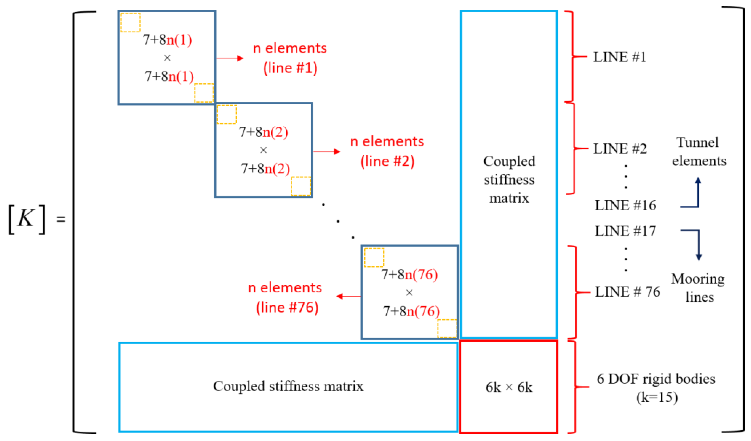
where and represent coupling stiffness and damping matrices, denotes a transformation matrix between the rigid body origin and the connection location, and are the displacements of the rigid body and the connecting location. Infinite stiffness values are used in the coupling stiffness matrix to tightly connect lines, and damping matrix is not utilized in the simulations. Therefore, the entire stiffness matrix that couples tunnel elements with mooring lines is created as shown in Figure 2.
Newton’s iteration method is used in static analysis of the SFT. The Adams–Moulton implicit integration method, which has 2nd-degree of accuracy, is used for the time-domain-integration method. Since instantaneous velocity and acceleration are required to calculate hydrodynamic force from Morison equation, the Adam–Bashforth explicit scheme is combined with the Adams–Moulton implicit scheme to avoid iteration.
3.2. Theory of OrcaFlex
A similar approach is used to model the whole structure in OrcaFlex, a well-known commercial program. The tunnel and mooring lines are modelled by line elements, and the line-element theory is based on the lumped mass method. The line element consists of a series of nodes and segments. Force properties are lumped in the node, which includes weight, buoyancy, and drag etc. Stiffness components i.e., axial, bending, and torsional stiffness, are represented by massless springs [44]. The equation of motion is expressed in Equation (27).
where , , and are mass, damping, and stiffness matrices. is external force vector, which is hydrodynamic force in this case. Symbols, , , , and denote position, velocity, acceleration vectors, and time, respectively. Hydrodynamic force is also computed by the same Morison equation for a moving object with consideration for relative velocity and acceleration. The advantage of the developed program compared to OrcaFlex for the present application can be summarized as follows: (i) In OrcaFlex, hydrodynamic force generated from the seaquake effects is not included. (ii) In CHARM3D, higher-order rod FE elements are used compared to lumped-mass-based OrcaFlex. (iii) The seabed movements can be directly imputed in the developed program.
3.3. Environmental Conditions
Simultaneous random-wave and seismic excitations are considered for global performance analysis. The same wave and seismic time histories are inputted in both programs for cross-checking. JONSWAP wave spectrum is used to generate time histories of random waves. Significant wave height and peak period for the 100-year-storm condition are 11.7 m and 13.0 s. Enhancement parameter is 2.14 that is the average value in Korea [45]. Random waves are generated by superposing 100 component waves with randomly perturbed frequency intervals to avoid signal repetition. The lowest and highest cut-off frequencies of input spectrum is 0.3 rad/s and 2.3 rad/s, respectively. The wave direction is perpendicular to a longitudinal direction of the tunnel. A 3-h simulation is carried out to analyze the statistics of dynamic behaviors and mooring tensions under the storm condition. Figure 3 shows theoretical JONSWAP wave spectrum and the reproduced spectrum from the time histories of wave elevation. It also shows the time histories of wave elevation produced by the JONSWAP wave spectrum.
Regular (sinusoidal) and recorded irregular seismic excitations data are also employed. The amplitude of regular seismic motion in the vertical direction is 0.01 m at diverse frequencies from 0.781 rad/s to 7.805 rad/s. Figure 4 shows the time histories of seismic displacements and corresponding spectra for recorded irregular seismic excitations in three directions, which are obtained by USGS [46]. The earthquake occurred in 78 km WNW of Ferndale, California, USA in 2014, and the magnitude of this earthquake is 6.8 in Richter scale. Seismic displacements in three directions are inputted for each anchor point of mooring lines and two ends of the tunnel fixture at every time step. Hydrodynamic force from the seaquake effect is also computed for the tunnel and mooring lines.
4. Results and Discussions
4.1. Static Analysis
The developed code is first cross-checked with OrcaFlex in the static condition before dynamic simulations. Because static displacements of the tunnel are only affected by weight, buoyancy, and stiffness components of tunnel and mooring lines, direct comparison can be made after initial modeling of the entire SFT system. Figure 5 shows the vertical displacements of tunnel and mooring tension in the static condition. The results produced by the developed program coincide well with OrcaFelx’s results. The reference dashed line in the tension figure indicates the allowable tension (minimum break load divided by safety factor).
4.2. Dynamic Behaviors under Extreme Wave Excitations
Dynamic simulations under the 100-year-strom condition (Hs = 11.7 m and Tp = 13.0 s) are performed for three hours. As mentioned before, the same wave time histories are inputted to both programs to directly compare the dynamics results. Both computer programs produce almost identical results. Figure 6 shows the envelopes of maximum and minimum for SFT displacements and mooring tension. The maximum horizontal and vertical responses and mooring tension occur in the middle location. The horizontal responses are larger than the vertical responses since the 1st natural frequency of horizontal motion is closer to the input wave spectrum than that of vertical motion. Mooring-tension results show that shorter mooring lines (Line #3) have higher mooring tension than longer mooring lines (Line #1). The maximum mooring tension at the middle section is smaller than the MBL (minimum breaking load) divided by the SF (safety factor), which is presented in Figure 6b as a pink line. Recall that the MBL is 30,689 kN for Grade R5, which is obtained by DNV regulation [33]. The SF 1.67 is used as recommended by API RP 2SK [47]. Even if the extreme 100-year-storm condition is considered, the maximum mooring tension is still smaller than the allowable tension.
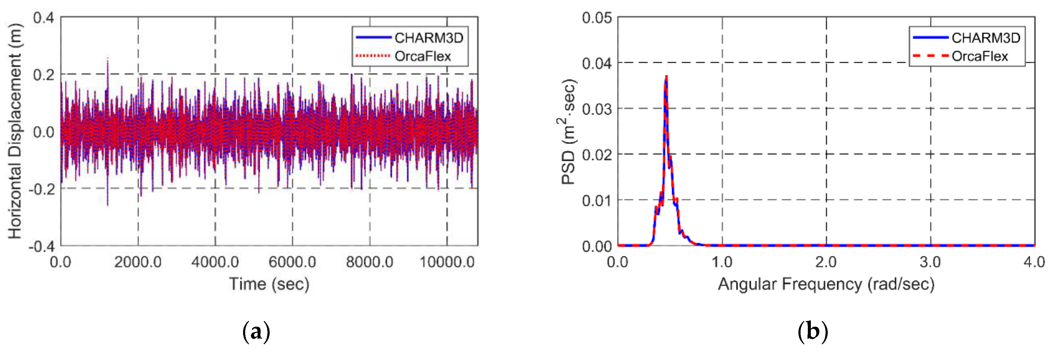
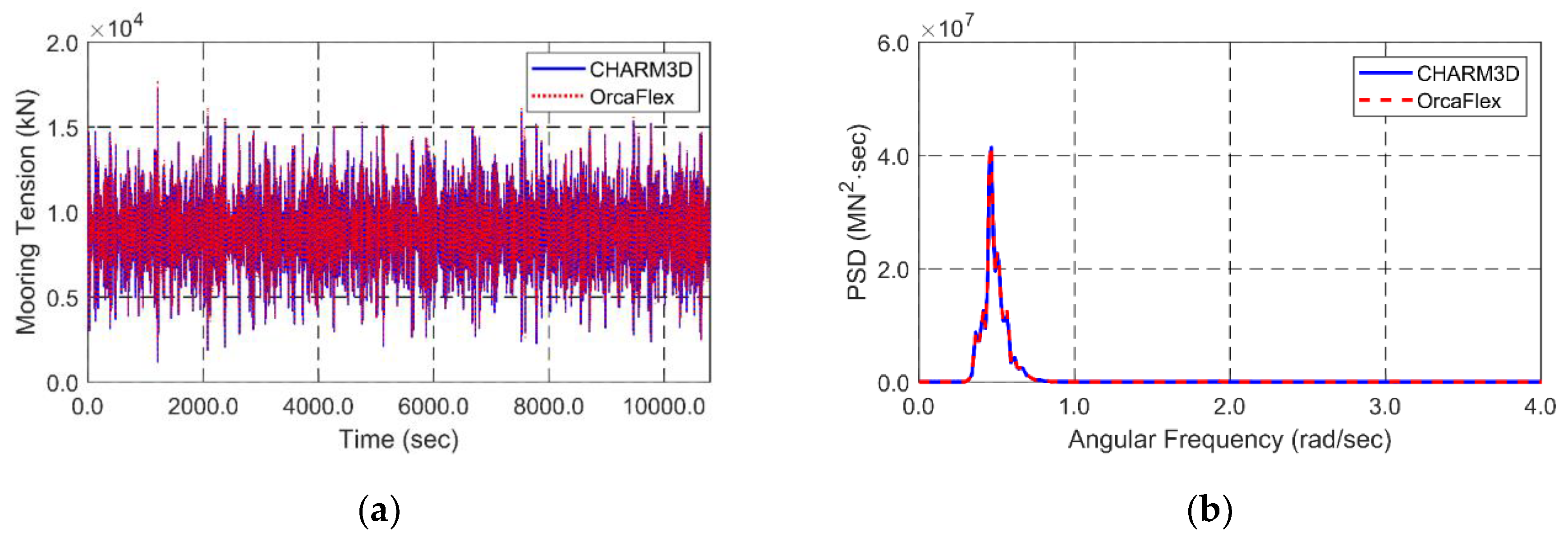
Figure 7, Figure 8 and Figure 9 show the time histories and corresponding spectra of horizontal/vertical responses of the tunnel and mooring tension at the middle section. The spectra of responses indicate that wave-induced motions are dominant since the lowest natural frequencies in both directional motions (1.92 and 3.12 rad/s for horizontal and vertical directions) are away from the dominant input-wave spectral range of Figure 3. It means that there is negligible contribution from the structural elastic resonances. In case of mooring tension, under the given BWR = 1.3, snap-loadings characterized by extraordinary high peaks do not occur, as shown in the time series. However, it should be noted that the snap-loadings tend to occur at lower BWRs [28]. Obviously, smaller dynamic motions and mooring tensions can be obtained by further increasing submergence depth [28]. The relevant statistics obtained from the time series are summarized in Table 3.
4.3. Dynamic Behaviors under Severe Seismic Excitations
Regular and irregular seismic excitations are utilized for SFT dynamic analysis. Since the fixed–fixed boundary condition is applied at both ends of the tunnel, both ends as well as all anchoring points are assumed to move together with seismic motions. As a result, seismic time histories are inputted to every anchor location of mooring lines and both ends of the tunnel. The hydrodynamic forces generated by sea-water fluctuations under vertical seismic motions are computed by using modified Morison equation (e.g., Islam and Ahrnad [41], Martinelli et al. [24], Mousavi et al. [42], and Wu et al. [25]). The effect is well known and called seaquake. As a result, there are two mechanisms causing SFT dynamics under seabed seismic motions. First, the seismic motions are transferred through mooring lines. Second, sea-water fluctuations in the vertical direction. In this paper, the former will be called earthquake effect and the latter will be called seaquake effect. To investigate the seaquake effect, regular seismic cases only in the vertical direction are simulated and the resulting SFT dynamics are analyzed. Subsequently, strong real seismic displacements are applied to the SFT system to check the global performance and structural robustness.
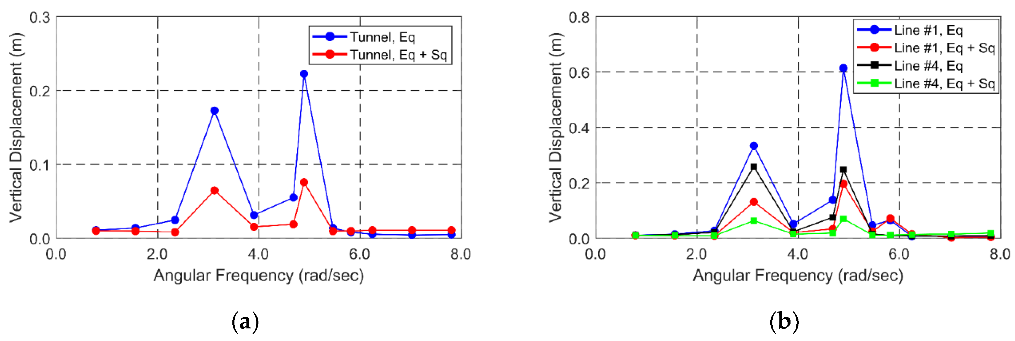
Figure 10 shows tunnel’s vertical motion amplitudes at the mid-section and the corresponding vertical responses of mooring line #1 at its center under regular (sinusoidal) seismic excitations. Vertical motions of tunnel are largely amplified at 3.12 rad/s and 4.89 rad/s, the 1st and 3rd natural frequencies. The amplified tunnel motions at those frequencies directly influence high mooring dynamics, as shown in Figure 10b. A small peak can also be observed at 5.78 rad/s, the lowest natural frequency of mooring lines #1 itself.
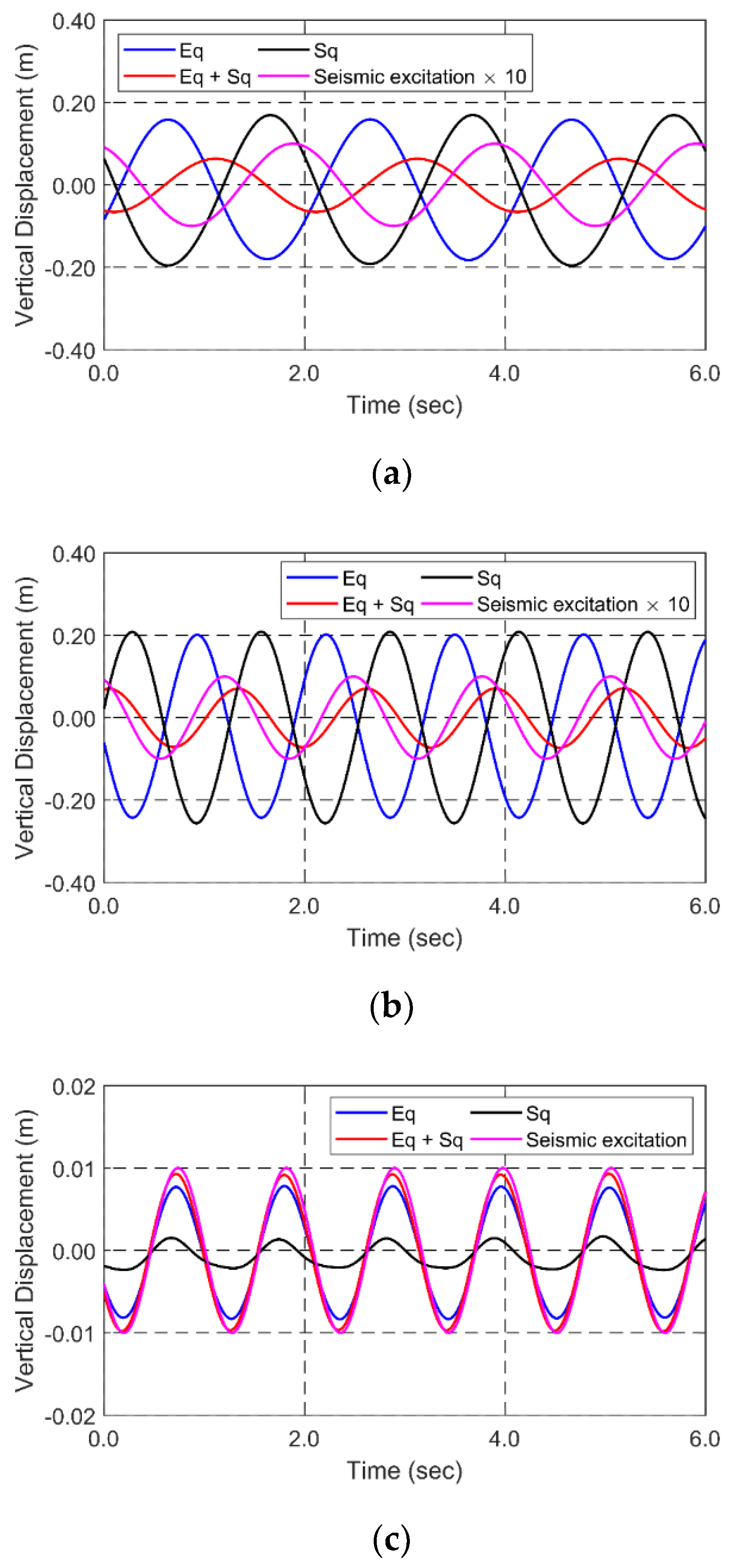
The hydrodynamic force by seaquake directly acts on the tunnel with earthquake frequencies. Whereas, the seismic excitations are delivered to the tunnel through mooring lines, as discussed earlier. Then, the resulting tunnel response also causes hydrodynamic force on the tunnel. Therefore, there exist phase effects between the two components. We can see that the tunnel dynamics are significantly reduced after including the seaquake effect when compared to the earthquake-only case. The reason can be found from Figure 11 by plotting the contribution of each constituent component separately. In the figure, the phase of the tunnel response induced by earthquake is opposite to that induced by seaquake at the tunnel’s natural frequencies, 3.12 rad/s and 4.89 rad/s. Therefore, there is cancellation effect between the two components so that the total vertical response amplitude can be reduced compared to the earthquake-only case. On the other hand, when earthquake frequency is greater than 5.7 rad/s, the two components become in phase, so the tunnel vertical responses are increased compared to the earthquake-only case although the resulting increment is small. The seaquake effects are not generated by the horizontal seismic motions if the seabed is flat since the horizontal seabed motions do not influence seawater fluctuating motions.
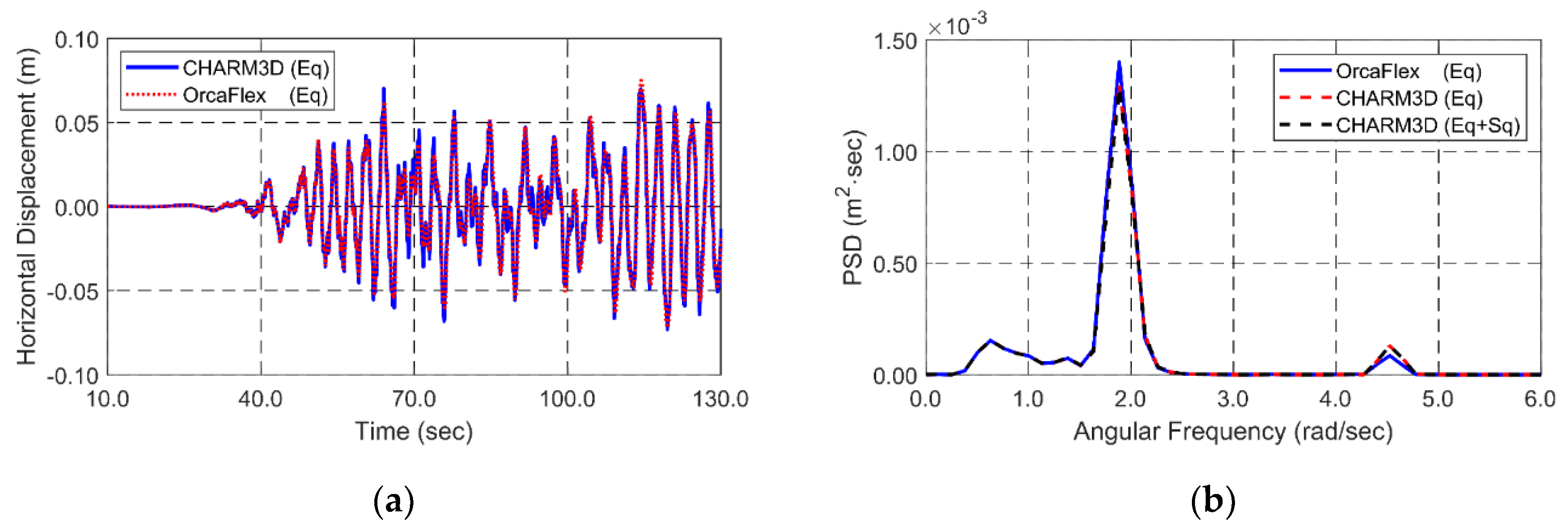
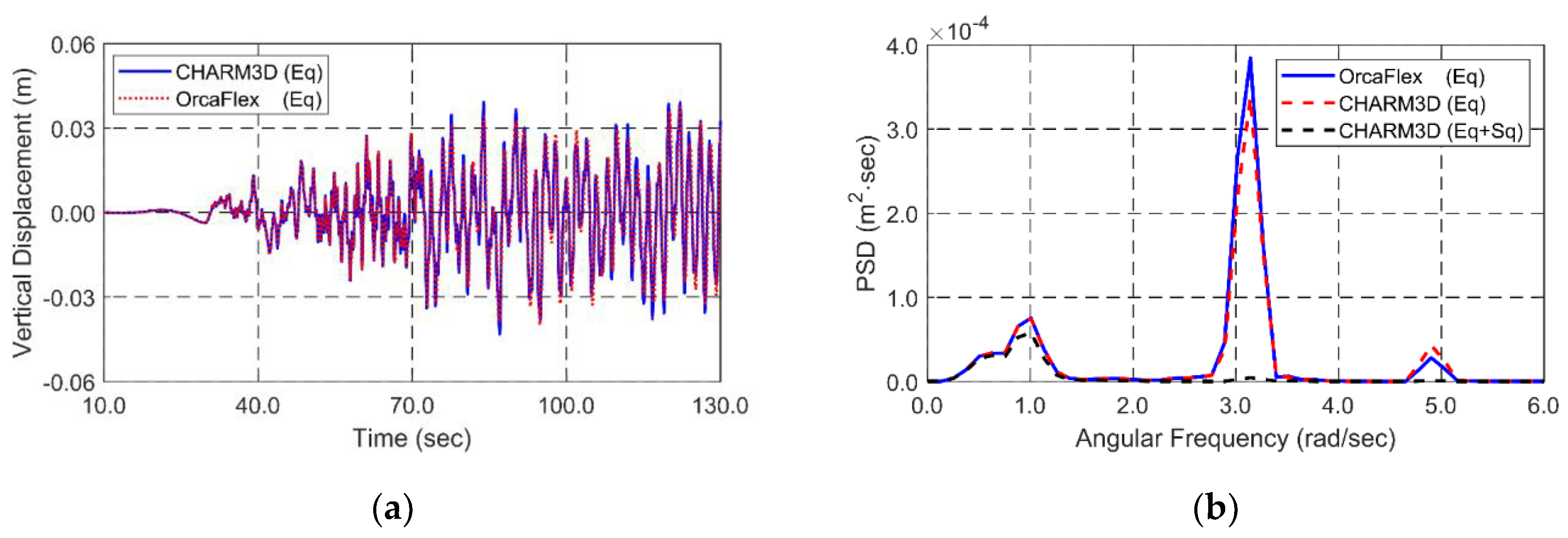
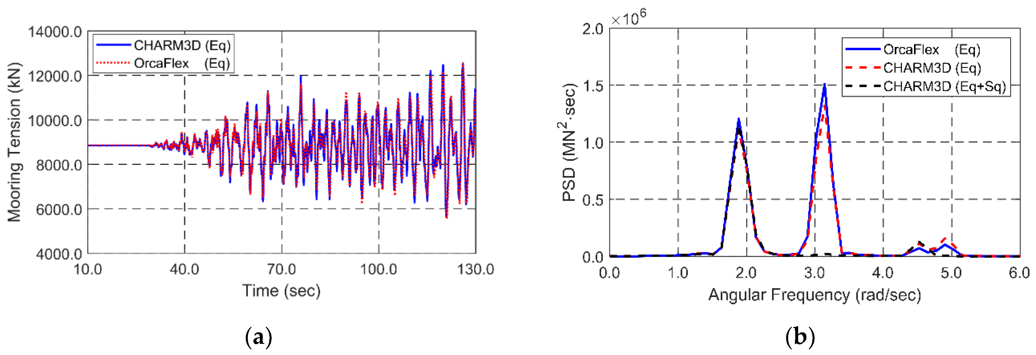
Figure 12, Figure 13 and Figure 14 show the time histories of horizontal/vertical responses of the tunnel and the corresponding mooring tensions at the tunnel’s middle section under the real seismic excitations, as given in Figure 4. The case of earthquake effect only is compared with that of earthquake plus seaquake. Firstly, in the earthquake-only case, the tunnel responses are greater than the input seismic motions, horizontally about 3 times and vertically about twice larger. The horizontal responses are more amplified because its lowest natural frequency is closer to the dominant frequency range of seismic excitations than that of vertical response. The corresponding tunnel-response spectra show that they have the first small peak at the seismic frequency, the next highest peak at the lowest natural frequency, and the next small peak at the third-lowest natural frequency. Mooring tensions are mostly influenced by the SFT horizontal and vertical motions at their lowest natural frequencies, while there is virtually little contribution near seismic frequencies. The maximum tensions for this earthquake case are much smaller than those caused by extreme wave excitations, as previously considered. However, the earthquake-induced tunnel dynamics can be significantly more amplified when the lowest natural frequencies of the tunnel’s elastic responses are closer to dominant seismic frequencies. In the figure, the same dynamic simulation results by OrcaFlex are also given for cross-checking. The two independent computer programs produced almost identical results.
In the spectral plots of Figure 12, Figure 13 and Figure 14, the spectra of tunnel responses and mooring tensions after adding seaquake effects are also given. In Figure 12, there is little change in the case of SFT horizontal motions since the seaquake mainly influences only the vertical responses, as was pointed out earlier. In Figure 13, there is a big reduction in the vertical-response spectrum at its lowest natural frequency (3.12 rad/s) after including the seaquake effect. It is due to the phase-cancellation effects, as discussed in the previous regular-earthquake case of Figure 11a,b. So, this reduction effect directly reflects the reduction in tension i.e., in Figure 14, the tension spectral amplitude is greatly reduced near 3.12 rad/s but remains the same at the lowest natural frequency of horizontal response, 1.92 rad/s. This trend can also be seen in the corresponding time-series comparisons (Figure 15) for the two cases (with and without considering the seaquake effect) regarding vertical tunnel responses and mooring tensions. The relevant statistics obtained from the time series are summarized in Table 4. It is seen that the inclusion of seaquake effect reduces both vertical SFT responses and mooring tensions, as discussed earlier.
5. Conclusions
Global performance analysis of the SFT was carried out for survival random wave and seismic excitations. To solve tunnel-mooring coupled hydro-elastic responses, an in-house time-domain- simulation computer program was developed. The hydro-elastic equation of motion for the tunnel and mooring was based on rod-theory-based finite element formulation with Galerkin method. The dummy-connection-mass method was devised to conveniently connect multiple segmented objects and mooring lines with linear and rotational springs. Considering the slender shape of the structure, hydrodynamic forces were computed by the modified Morison equation. The numerical results produced by the developed program were in good agreement with those by the commercial program OrcaFlex based on lumped-mass method. The extreme wave excitations caused the maximum SFT dynamic motions of 24 cm and 6 cm in the horizontal and vertical directions and the corresponding mooring tensions below allowable level. Snap motions and loadings of mooring lines were not observed. Under regular seismic excitations, large resonant responses of the tunnel were observed at 1st and 3rd natural frequencies. In the case of seabed earthquake, the seabed motions are transferred to SFT through mooring lines and through seawater fluctuations called seaquake. When the latter is further considered, horizontal responses were not affected but vertical responses become significantly reduced especially at its lowest natural frequency. After analyzing the behaviors of the two contributions, it was found that the reduction was caused by the phase-cancellation effect. However, in other cases, the phases could enhance each other to increase the total responses of the SFT. Under extreme irregular seismic excitations, the maximum SFT dynamic motions of 7 cm and 2 cm were generated and the corresponding mooring tensions were about 30% smaller compared to the extreme wave case. However, when the frequencies of seismic excitations are closer to SFT natural frequencies, larger dynamic amplifications are expected.
Author Contributions
All authors have equally contributed to publish this article related to design of target model, validation of numerical modeling, simulations, analysis, and writing.
Funding
This work was supported by the National Research Foundation of Korea (NRF) grant funded by the Korea government (MSIT) (No. 2017R1A5A1014883).
Conflicts of Interest
The authors declare no conflict of interest.
References
- Ge, F.; Lu, W.; Wu, X.; Hong, Y. Fluid-structure interaction of submerged floating tunnel in wave field. Procedia Eng. 2010, 4, 263–271. [Google Scholar] [CrossRef]
- Paik, I.Y.; Oh, C.K.; Kwon, J.S.; Chang, S.P. Analysis of wave force induced dynamic response of submerged floating tunnel. KSCE J. Civ. Eng. 2004, 8, 543–550. [Google Scholar] [CrossRef]
- Long, X.; Ge, F.; Wang, L.; Hong, Y. Effects of fundamental structure parameters on dynamic responses of submerged floating tunnel under hydrodynamic loads. Acta Mech. Sin. 2009, 25, 335–344. [Google Scholar] [CrossRef]
- Di Pilato, M.; Perotti, F.; Fogazzi, P. 3D dynamic response of submerged floating tunnels under seismic and hydrodynamic excitation. Eng. Struct. 2008, 30, 268–281. [Google Scholar] [CrossRef]
- Faggiano, B.; Landolfo, R.; Mazzolani, F. The sft: An innovative Solution for waterway Strait Crossings; IABSE Symposium Report; International Association for Bridge and Structural Engineering: Lisbon, Portugal, 2005; pp. 36–42. [Google Scholar]
- Muhammad, N.; Ullah, Z.; Choi, D.-H. Performance evaluation of submerged floating tunnel subjected to hydrodynamic and seismic excitations. Applied Sci. 2017, 7, 1122. [Google Scholar] [CrossRef]
- Skorpa, L. Innovative norwegian fjord crossing. How to cross the høgsjord, alternative methods. In Proceedings of the 2nd Congress AIOM (Marine and Offshore Engineering Association), Naples, Italy, 15–17 November 1989; pp. 15–17. [Google Scholar]
- Remseth, S.; Leira, B.J.; Okstad, K.M.; Mathisen, K.M.; Haukås, T. Dynamic response and fluid/structure interaction of submerged floating tunnels. Comput. Struct. 1999, 72, 659–685. [Google Scholar] [CrossRef]
- Engebretsen, K.B.; Jakobsen, K.K.; Haugerud, S.A.; Minoretti, A. A submerged floating tube bridge concept for the bjørnafjord crossing: Marine operations. In Proceedings of the ASME 2017 36th International Conference on Ocean, Offshore and Arctic Engineering, Trondheim, Norway, 25–30 June 2017; American Society of Mechanical Engineers: New York, NY, USA, 2017; p. V07BT06A027. [Google Scholar]
- Faggiano, B.; Landolfo, R.; Mazzolani, F. Design and modelling aspects concerning the submerged floating tunnels: An application to the messina strait crossing. Krobeborg. Strait Crossing 2001, 511–519. [Google Scholar]
- Lu, W.; Ge, F.; Wang, L.; Wu, X.; Hong, Y. On the slack phenomena and snap force in tethers of submerged floating tunnels under wave conditions. Mar. Struct. 2011, 24, 358–376. [Google Scholar] [CrossRef]
- Fujii, T. Submerged floating tunnels project in funka bay design and execution. In Proceedings of the International Conference on Submerged Floating Tunnel, Sandnes, Norway, 29–30 May 1996. [Google Scholar]
- Martinelli, L.; Barbella, G.; Feriani, A. A numerical procedure for simulating the multi-support seismic response of submerged floating tunnels anchored by cables. Eng. Struct. 2011, 33, 2850–2860. [Google Scholar] [CrossRef]
- Mazzolani, F.; Landolfo, R.; Faggiano, B.; Esposto, M.; Perotti, F.; Barbella, G. Structural analyses of the submerged floating tunnel prototype in qiandao lake (pr of china). Adv. Struct. Eng. 2008, 11, 439–454. [Google Scholar] [CrossRef]
- Han, J.S.; Won, B.; Park, W.-S.; Ko, J.H. Transient response analysis by model order reduction of a mokpo-jeju submerged floating tunnel under seismic excitations. Struct. Eng. Mech. 2016, 57, 921–936. [Google Scholar] [CrossRef]
- Lee, J.; Jin, C.; Kim, M. Dynamic response analysis of submerged floating tunnels by wave and seismic excitations. Ocean Syst. Eng. Int. J. 2017, 7, 1–19. [Google Scholar] [CrossRef]
- Ghimire, A.; Prakash, O. Intangible study for the design and construction of submerged floating tunnel. Imp. J. Interdiscip. Res. 2017, 3, 721–724. [Google Scholar]
- Kunisu, H.; Mizuno, S.; Mizuno, Y.; Saeki, H. Study on submerged floating tunnel characteristics under the wave condition. In Proceedings of the The Fourth International Offshore and Polar Engineering Conference, Osaka, Japan, 10–15 April 1994; International Society of Offshore and Polar Engineers: Osaka, Japan, 1994; pp. 27–32. [Google Scholar]
- Hong, Y.; Ge, F.; Lu, W. On the two essential concepts for sft: Synergetic buoyancy-weight ratio and slack-taut map. Procedia Eng. 2016, 166, 221–228. [Google Scholar] [CrossRef]
- Long, X.; Ge, F.; Hong, Y. Feasibility study on buoyancy–weight ratios of a submerged floating tunnel prototype subjected to hydrodynamic loads. Acta Mech. Sin. 2015, 31, 750–761. [Google Scholar] [CrossRef] [Green Version]
- Seo, S.-I.; Mun, H.-S.; Lee, J.-H.; Kim, J.-H. Simplified analysis for estimation of the behavior of a submerged floating tunnel in waves and experimental verification. Mar. Struct. 2015, 44, 142–158. [Google Scholar] [CrossRef]
- Chen, Z.; Xiang, Y.; Lin, H.; Yang, Y. Coupled vibration analysis of submerged floating tunnel system in wave and current. Appl. Sci. 2018, 8, 1311. [Google Scholar] [CrossRef]
- Xiao, J.; Huang, G. Transverse earthquake response and design analysis of submerged floating tunnels with various shore connections. Procedia Eng. 2010, 4, 233–242. [Google Scholar] [CrossRef]
- Martinelli, L.; Domaneschi, M.; Shi, C. Submerged floating tunnels under seismic motion: Vibration mitigation and seaquake effects. Procedia Eng. 2016, 166, 229–246. [Google Scholar] [CrossRef]
- Wu, Z.; Ni, P.; Mei, G. Vibration response of cable for submerged floating tunnel under simultaneous hydrodynamic force and earthquake excitations. Adv. Struct. Eng. 2018, 21, 1761–1773. [Google Scholar] [CrossRef]
- Mirzapour, J.; Shahmardani, M.; Tariverdilo, S. Seismic response of submerged floating tunnel under support excitation. Ships Offshore Struct. 2017, 12, 404–411. [Google Scholar] [CrossRef]
- Cifuentes, C.; Kim, S.; Kim, M.; Park, W. Numerical simulation of the coupled dynamic response of a submerged floating tunnel with mooring lines in regular waves. Ocean Syst. Eng. 2015, 5, 109–123. [Google Scholar] [CrossRef]
- Jin, C.; Kim, M. Dynamic and structural responses of a submerged floating tunnel under extreme wave conditions. Ocean Syst. Eng. Int. J. 2017, 7, 413–433. [Google Scholar]
- Jin, C.; Lee, J.; Kim, H.; Kim, M. Dynamic responses of a submerged floating tunnel in survival wave and seismic excitations. In Proceedings of the The 27th International Ocean and Polar Engineering Conference, San Francisco, CA, USA, 25–30 June 2017; International Society of Offshore and Polar Engineers: San Francisco, CA, USA, 2017; pp. 547–551. [Google Scholar]
- Lee, J.H.; Seo, S.I.; Mun, H.S. Seismic behaviors of a floating submerged tunnel with a rectangular cross-section. Ocean Eng. 2016, 127, 32–47. [Google Scholar] [CrossRef]
- Thompson, N. Mean forces, pressure and flow field velocities for circular cylindrical structures: Single cylinder with two-dimensional flow. EDU Data Item 1980, 80025. [Google Scholar]
- Veritas, D.N. Offshore Standard dnv-os-e301: Offshore Standard-Position Mooring; Det Norske Veritas (DNV) Oslo: Oslo, Norway, 2010. [Google Scholar]
- Veritas, D.N. Offshore Standard dnv-os-e302: Offshore Mooring Chain; Det Norske Veritas (DNV) Oslo: Oslo, Norway, 2009. [Google Scholar]
- Kim, M.; Koo, B.; Mercier, R.; Ward, E. Vessel/mooring/riser coupled dynamic analysis of a turret-moored fpso compared with otrc experiment. Ocean Eng. 2005, 32, 1780–1802. [Google Scholar] [CrossRef]
- Koo, B.; Kim, M. Hydrodynamic interactions and relative motions of two floating platforms with mooring lines in side-by-side offloading operation. Appl. Ocean Res. 2005, 27, 292–310. [Google Scholar] [CrossRef]
- Bae, Y.; Kim, M. Coupled dynamic analysis of multiple wind turbines on a large single floater. Ocean Eng. 2014, 92, 175–187. [Google Scholar] [CrossRef]
- Kim, S.; Kim, M.; Kang, H. Turret location impact on global performance of a thruster-assisted turret-moored fpso. Ocean Syst. Eng. Int. J. 2016, 6, 265–287. [Google Scholar] [CrossRef]
- Jang, H.; Kang, H.; Kim, M. Numerical simulation of dynamic interactions of an arctic spar with drifting level ice. Ocean Syst. Eng. Int. J. 2016, 6, 345–362. [Google Scholar] [CrossRef]
- Garrett, D. Dynamic analysis of slender rods. J. Energy Resour. Technol. 1982, 104, 302–306. [Google Scholar] [CrossRef]
- Faltinsen, O. Sea Loads on Ships and Offshore Structures; Cambridge University Press: London, UK, 1993. [Google Scholar]
- Islam, N.; Ahrnad, S. Nonlinear seismic response of articulated offshore tower. Def. Sci. J. 2003, 53, 105–113. [Google Scholar] [CrossRef]
- Mousavi, S.A.; Bargi, K.; Zahrai, S.M. Optimum parameters of tuned liquid column–gas damper for mitigation of seismic-induced vibrations of offshore jacket platforms. Struct. Control Health Monit. 2013, 20, 422–444. [Google Scholar] [CrossRef]
- Ran, Z.; Kim, M.; Zheng, W. Coupled dynamic analysis of a moored spar in random waves and currents (time-domain versus frequency-domain analysis). J. Offshore Mech. Arct. Eng. 1999, 121, 194–200. [Google Scholar] [CrossRef]
- Orcina. Orcaflex Manual. Available online: https://www.orcina.com/SoftwareProducts/OrcaFlex/index.php (accessed on 17 October 2018).
- Suh, K.-D.; Kwon, H.-D.; Lee, D.-Y. Some statistical characteristics of large deepwater waves around the korean peninsula. Coast. Eng. 2010, 57, 375–384. [Google Scholar] [CrossRef]
- USGS. National Strong-Motion Project Earthquake Data Sets. Available online: https://escweb.wr.usgs.gov/nsmp-data/nsmn_eqdata.html (accessed on 27 August 2018).
- API. Recommended Practice for Design and Analysis of Stationkeeping Systems for Floating Structures: Exploration and Production Department. Api Recommended Practice 2sk (rp 2sk): Effective Date: March 1, 1997; American Petroleum Institute: Washington, DC, USA, 1996. [Google Scholar]
Figure 1.
2D and 3D views of the entire structure.

Figure 2.
Stiffness matrix for the simulated SFT (line #1~#16 are for tunnel and line #17~#N are for mooring lines, n(1) means number of sub-elements of line #1, k is the number of the 6 DOF rigid body).
Figure 2.
Stiffness matrix for the simulated SFT (line #1~#16 are for tunnel and line #17~#N are for mooring lines, n(1) means number of sub-elements of line #1, k is the number of the 6 DOF rigid body).

Figure 3.
Wave time histories produced by JONSWAP wave spectrum (a) and theoretical JONSWAP wave spectrum and reproduced spectrum from wave time histories using FFT (fast Fourier transform) for validation (b).
Figure 3.
Wave time histories produced by JONSWAP wave spectrum (a) and theoretical JONSWAP wave spectrum and reproduced spectrum from wave time histories using FFT (fast Fourier transform) for validation (b).

Figure 4.
Time histories of real seismic excitations in longitudinal = x (a), transverse = y (b), and vertical = z (c) directions and its corresponding spectra.
Figure 4.
Time histories of real seismic excitations in longitudinal = x (a), transverse = y (b), and vertical = z (c) directions and its corresponding spectra.

Figure 5.
Submerged floating tunnel (SFT) vertical displacement (a) and mooring tension (b) in the static condition.
Figure 5.
Submerged floating tunnel (SFT) vertical displacement (a) and mooring tension (b) in the static condition.

Figure 6.
Envelopes of the maximum and minimum displacements of the tunnel (a) and mooring tension (b) in the 100-year-strom condition.
Figure 6.
Envelopes of the maximum and minimum displacements of the tunnel (a) and mooring tension (b) in the 100-year-strom condition.

Figure 7.
Time histories (a) and spectrum (b) of horizontal displacement of the tunnel in the middle location under the 100-year-strom waves.
Figure 7.
Time histories (a) and spectrum (b) of horizontal displacement of the tunnel in the middle location under the 100-year-strom waves.

Figure 8.
Time histories (a) and spectrum (b) of vertical displacement of the tunnel in the middle location under the 100-year-strom waves.
Figure 8.
Time histories (a) and spectrum (b) of vertical displacement of the tunnel in the middle location under the 100-year-strom waves.

Figure 9.
Time histories (a) and spectrum (b) of mooring tension (#3) in the middle location under the 100-year-strom waves.
Figure 9.
Time histories (a) and spectrum (b) of mooring tension (#3) in the middle location under the 100-year-strom waves.

Figure 10.
Amplitudes of vertical displacements of the tunnel (a) and mooring line #1 (b) at the middle location under regular seismic excitations of various frequencies (Eq: earthquake only considered; Eq + Sq: both earthquake and seaquake considered).
Figure 10.
Amplitudes of vertical displacements of the tunnel (a) and mooring line #1 (b) at the middle location under regular seismic excitations of various frequencies (Eq: earthquake only considered; Eq + Sq: both earthquake and seaquake considered).

Figure 11.
Time histories of vertical displacements of the tunnel at the middle section by respective force components under regular seismic excitations of 3.12 rad/s (a), 4.89 rad/s (b), and 5.78 rad/s (c) (Eq: earthquake only considered; Eq + Sq: both earthquake and seaquake considered; Sq: seaquake only considered; time histories of seismic excitations are multiplied by 10 for better visualization).

Figure 12.
Time histories (without seaquake) (a) and spectra (b) of horizontal tunnel responses at the middle location under seismic excitations
Figure 12.
Time histories (without seaquake) (a) and spectra (b) of horizontal tunnel responses at the middle location under seismic excitations

Figure 13.
Time histories (without seaquake) (a) and spectra (b) of vertical tunnel responses at the middle location under seismic excitations.
Figure 13.
Time histories (without seaquake) (a) and spectra (b) of vertical tunnel responses at the middle location under seismic excitations.

Figure 14.
Time histories (without seaquake) (a) and spectra (b) of mooring tension #4 at the middle location under seismic excitations
Figure 14.
Time histories (without seaquake) (a) and spectra (b) of mooring tension #4 at the middle location under seismic excitations

Figure 15.
Time histories of vertical responses of the tunnel (a) and mooring tension #4 (b) in the middle location under seismic excitations with and without seaquake effect.
Figure 15.
Time histories of vertical responses of the tunnel (a) and mooring tension #4 (b) in the middle location under seismic excitations with and without seaquake effect.


Table 1.
Major parameters of the tunnel and mooring lines.
| Component | Parameter | Value | Unit |
|---|---|---|---|
| Tunnel | Length | 700 | m |
| Outer diameter | 23 | m | |
| End boundary condition | Fixed-fixed condition | - | |
| Material | High-density concrete | - | |
| Young’s modulus | 30 | GPa | |
| Bending stiffness (EI) | 2.34 × 10¹¹ | kN·m2 | |
| Axial stiffness (EA) | 4.27 × 10⁹ | kN | |
| Buoyancy-weight ratio (BWR) | 1.3 | - | |
| Added mass coefficient | 1.0 | - | |
| Drag coefficient | 0.55 [31] | - | |
| Mooring lines (Chain, Stud-less type) | Length | 51.1 (Line # 1 and 2), 37.8 (Line # 3 and 4) | m |
| Mass/unit length | 644.7 | kg/m | |
| Nominal diameter () for wave drag force calculation | 0.18 | m | |
| Equivalent outer diameter () for wave inertia force calculation | 0.324 () | m | |
| Bending stiffness () | 0 | kN·m2 | |
| Axial stiffness () | 2.77 × 10⁶ | kN | |
| Added mass coefficient | 1.0 | ||
| Drag coefficient | 2.4 [32] | ||
| Minimum breaking load (MBL) | 30,689 (Grade R5) [33] | kN |
Table 2.
Wet natural frequencies of the tunnel hydro-elastic responses coupled with mooring lines.
| Component | Wet Natural Frequency (rad/s) | Mode Number |
|---|---|---|
| Tunnel (Horizontal direction) | 1.92 | 1st mode |
| 2.70 | 2nd mode | |
| 4.53 | 3rd mode | |
| Tunnel (Vertical direction) | 3.12 | 1st mode |
| 3.45 | 2nd mode | |
| 4.89 | 3rd mode | |
| Mooring lines #1 and #2 (Center) | 5.78 | 1st mode |
| Mooring lines #3 and #4 (Center) | 9.04 | 1st mode |
Table 3.
Statistics of the SFT motions and mooring tensions at the middle location under 100-yr irregular wave excitations (from the time series of Figure 7, Figure 8 and Figure 9).
| Parameter | Maximum | Minimum | Standard Deviation | Unit |
|---|---|---|---|---|
| Horizontal displacement | 0.243 | −0.261 | 0.059 | m |
| Vertical displacement | 0.058 | −0.066 | 0.014 | |
| Mooring tension (line #1) | 14,765.75 | 885.56 | 1917.55 | kN |
| Mooring tension (line #2) | 15,276.12 | 902.94 | 1919.01 | |
| Mooring tension (line #3) | 17,334.93 | 1206.64 | 2015.53 | |
| Mooring tension (line #4) | 16,542.11 | 953.24 | 2014.32 |
Table 4.
Statistics of the SFT motions and mooring tensions at the middle location under irregular seismic excitations (Eq: earthquake, Sq: seaquake).
Table 4.
Statistics of the SFT motions and mooring tensions at the middle location under irregular seismic excitations (Eq: earthquake, Sq: seaquake).
| Parameter | Numerical Model | Maximum | Minimum | Standard Deviation | Unit |
|---|---|---|---|---|---|
| Horizontal displacement | Eq | 0.070 | −0.073 | 0.023 | m |
| Eq + Sq | 0.070 | −0.072 | 0.023 | ||
| Vertical displacement | Eq | 0.039 | −0.042 | 0.013 | |
| Eq + Sq | 0.019 | −0.019 | 0.006 | ||
| Mooring tension (line #1) | Eq | 9872.22 | 3783.56 | 801.58 | kN |
| Eq + Sq | 8728.01 | 4631.84 | 649.80 | ||
| Mooring tension (line #2) | Eq | 9722.09 | 3291.79 | 829.07 | |
| Eq + Sq | 8778.38 | 4491.79 | 649.33 | ||
| Mooring tension (line #3) | Eq | 12,295.18 | 4918.66 | 958.46 | |
| Eq + Sq | 11,009.40 | 6691.91 | 649.58 | ||
| Mooring tension (line #4) | Eq | 12,512.53 | 5633.35 | 925.67 | |
| Eq + Sq | 11,001.66 | 6772.99 | 652.55 |
© 2018 by the authors. Licensee MDPI, Basel, Switzerland. This article is an open access article distributed under the terms and conditions of the Creative Commons Attribution (CC BY) license (http://creativecommons.org/licenses/by/4.0/).
Share and Cite
MDPI and ACS Style
Jin, C.; Kim, M.-H. Time-Domain Hydro-Elastic Analysis of a SFT (Submerged Floating Tunnel) with Mooring Lines under Extreme Wave and Seismic Excitations. Appl. Sci. 2018, 8, 2386. https://doi.org/10.3390/app8122386
AMA Style
Jin C, Kim M-H. Time-Domain Hydro-Elastic Analysis of a SFT (Submerged Floating Tunnel) with Mooring Lines under Extreme Wave and Seismic Excitations. Applied Sciences. 2018; 8(12):2386. https://doi.org/10.3390/app8122386
Chicago/Turabian StyleJin, Chungkuk, and Moo-Hyun Kim. 2018. "Time-Domain Hydro-Elastic Analysis of a SFT (Submerged Floating Tunnel) with Mooring Lines under Extreme Wave and Seismic Excitations" Applied Sciences 8, no. 12: 2386. https://doi.org/10.3390/app8122386
Note that from the first issue of 2016, this journal uses article numbers instead of page numbers. See further details here.