CFD Investigation of a High Head Francis Turbine at Speed No-Load Using Advanced URANS Models

Featured Application

The present numerical investigation gives some insights regarding the challenges to compute the flow in hydraulic Francis turbines at off-design operating points. However, such simulations are useful to design hydraulic turbines that will be operated with more flexibility. Therefore, the present results can be used to determine which turbulence models are useful to compute off-design operating points, keeping in mind limitations and future improvements.

Abstract

Due to the integration of new renewable energies, the electrical grid undergoes instabilities. Hydroelectric power plants are key players for grid control thanks to pumped storage power plants. However, this objective requires extending the operating range of the machines and increasing the number of start-up, stand-by, and shut-down procedures, which reduces the lifespan of the machines. CFD based on standard URANS turbulence modeling is currently able to predict accurately the performances of the hydraulic turbines for operating points close to the Best Efficiency Point (BEP). However, far from the BEP, the standard URANS approach is less efficient to capture the dynamics of 3D flows. The current study focuses on a hydraulic turbine, which has been investigated at the BEP and at the Speed-No-Load (SNL) operating conditions. Several “advanced” URANS models such as the Scale-Adaptive Simulation (SAS) SST $k-\omega$ and the BSL- EARSM have been considered and compared with the SST $k-\omega$ model. The main conclusion of this study is that, at the SNL operating condition, the prediction of the topology and the dynamics of the flow on the suction side of the runner blade channels close to the trailing edge are influenced by the turbulence model.

1. Introduction

Hydropower is the main renewable source of energy generation in the world with 3.7% of the total final energy consumption [1]. In order to increase the part of the hydropower in the energy mix, efforts are made to develop micro-hydropower [2], to recover energy from existing water networks [3], or to improve the efficiency of the existing power plants during refurbishment [4]. Beyond these efforts and due to the development and integration of renewable energy resources, hydraulic turbines and pump-turbines are key technical components for load shifting and frequency control of the grid [5,6]. However, in order to act as a grid stabilizer, the hydraulic machines have to extend their operating range [7].

Computational Fluid Dynamics (CFD) is one of the main tools used to investigate the dynamics of the flow in various hydraulic turbines at both stable and unstable operating points [8,9]. Most of the numerical investigations are carried out by solving the Unsteady Reynolds-Averaged Navier–Stokes (URANS ) equations. The Reynolds stresses are often modeled using Boussinesq’s assumption, which requires computing the eddy viscosity, usually calculated using a two-equation turbulence model. Such an approach has been used to compute full head Francis turbines at the Best Efficiency Point (BEP) including also full load [10,11,12,13], partial load [13,14,15], and Speed-No-Load (SNL) [16,17,18] operating points or transition from pump to turbine mode [19], start-up [20], or the S-shaped region of pump-turbines [21]. The Francis-99 workshop, whose summary is available in [22,23], gave an overview of the state of the art for the simulation of high head Francis turbines at design and off-design operating points. Regarding the turbulence modeling, the authors mentioned that the BEP is well predicted by both URANS and hybrid turbulence models. The part load operating point is more challenging, and results show a larger discrepancy compared to the measurements. This discrepancy is explained by the influence of the mesh near the wall boundaries. Hybrid turbulence models improve the results at part load operating conditions compared to the standard URANS models.

Regarding more precisely the SNL operating conditions, several authors put in evidence the inability of standard two-equation turbulence models to capture the pressure fluctuations [17,18]. Indeed, these models are built to compute steady flows in absence of streamline curvature, stagnation points and large vortices, which are characteristic of the flow at SNL. Therefore, in order to overcome the limitations of the standard turbulence models, Scale-Adaptive Simulation (SAS) [17] based on the Shear Stress Transport (SST) $k-\omega$ model or Large Eddy Simulation (LES) [18] has been carried out. In both cases, the content in pressure fluctuations is enhanced and shows an improved agreement with the experimental measurements.

LES in a complete hydraulic machine requires a very fine mesh with around 100 million nodes [18,24]. In order to avoid the use of such large meshes, which require large Central Processing Unit (CPU) resources, some authors intended to use hybrid RANS/LES models. Hybrid RANS/LES models are designed to adjust the level of the eddy viscosity in relation to the grid spacing, at least in the framework of Detached Eddy Simulation (DES) [25,26]. Krappel et al. [27] used the Improved Delayed-Detached Eddy Simulation (IDDES) model to simulate the flow in a Francis pump turbine with a mesh containing 20 million elements. Compared to the results provided by the SST $k-\omega$ turbulence model, the IDDES model improved the prediction of the standard deviation of the velocity components and of the turbulent kinetic energy in the draft tube cone. Minakov et al. computed the part load and full load operating conditions in a reduced domain of the Francis-99 turbine using a DES SST $k-\omega$ model and a mesh with only six million control volumes [28]. The results show an improvement of the accuracy regarding the r.m.s. velocity components compared to the results provided by a standard Reynolds stress model. The LES behavior can also be obtained without using explicitly the grid spacing, as is the case in the SAS framework proposed by Menter and Egorov [29,30]. The SAS formulation has been used by several authors to compute the flow through hydraulic turbines [17,31]. Neto et al. [31] showed that the SAS model on a grid with nine million control volumes improves the prediction of the velocity profiles in the draft tube diffuser for the part load operating condition compared to the standard SST model. Excluding the resolution of the turbulent eddies, Explicit Algebraic Reynolds Stress Models (EARSM) and Reynolds Stress Models (RSM) are able to capture the flows characterized by stagnation points and streamline curvature. Such models have been used for instance by Mössinger et al. [32] to compute the flow in a high head Francis turbine including part load, BEP, and full load operating conditions. They concluded that the EARSM or RSM model does not improve the results compared to the SST model. Moreover, at part load condition, the RSM model was not able to converge.

Based on the previous literature review, the linear eddy viscosity models are able to compute accurately the BEP of a high head Francis turbine, but have some difficulties in computing the flow at part load and SNL operating conditions. During the last 15 years, several improvements have been achieved in the development of URANS and hybrid RANS/LES models [33,34,35]. Consequently, the present paper focuses on the influence of some “advanced” URANS turbulence models regarding the dynamics of the flow at the SNL operating condition of a high head Francis turbine already investigating at part load by Müller et al. [36] and at various operating points by the current authors [37,38,39].

The paper deals first with the description of the case study, the governing equations, and the numerical setup. In the BEP results, a detailed analysis regarding the influence of the mesh, the boundary conditions, and the numerical setup is carried out. Finally, the SNL operating point is computed with four “advanced” URANS models: the SST $k-\omega$ model with production limiter and curvature correction, the SAS SST $k-\omega$ model, the Organised Eddy Simulation (OES) SST $k-\omega$ model, and the Baseline $k-\omega$ model (BSL) EARSM model. The results are compared with the ones provided by the standard SST $k-\omega$ model and with experimental data.

2. Case Study

The considered case study is the Grimsel 2 pumped-storage power plant operated by Kraftwerke Oberhasli AG (KWO) [40] and built between 1974 and 1980 in Switzerland. This power plant is equipped with four 100-MW ternary groups: a horizontal-axis motor/generator, a Francis turbine, and a pump. The number of guide vanes is $z_g=24$, and the number of runner blades is $z_b=17$. The speed, discharge, and power factors along with the specific speed at the BEP are respectively:

$$\begin{array}{cccccccc}\hfill n_{ED}=& \frac{nD}{E^{1/2}}=0.271\hfill & \hfill Q_{ED}=& \frac{Q}{D^2{E}^{1/2}}=0.183\hfill & \hfill P_{ED}=& \frac{P_m}{\rho D^2{E}^{3/2}}=0.171\hfill & \hfill \nu =& \frac{\omega Q^{1/2}}{{\pi }^{1/2}{\left(2E\right)}^{3/4}}=0.247\hfill \end{array}$$

(1)

At the BEP, the Reynolds number is equal to $21.6\times {10}^6$ based on the discharge velocity and the diameter at the runner outlet section (these two quantities are used to define the dimensionless variables in the paper. The dimensionless pressure is defined with the head at the BEP.).

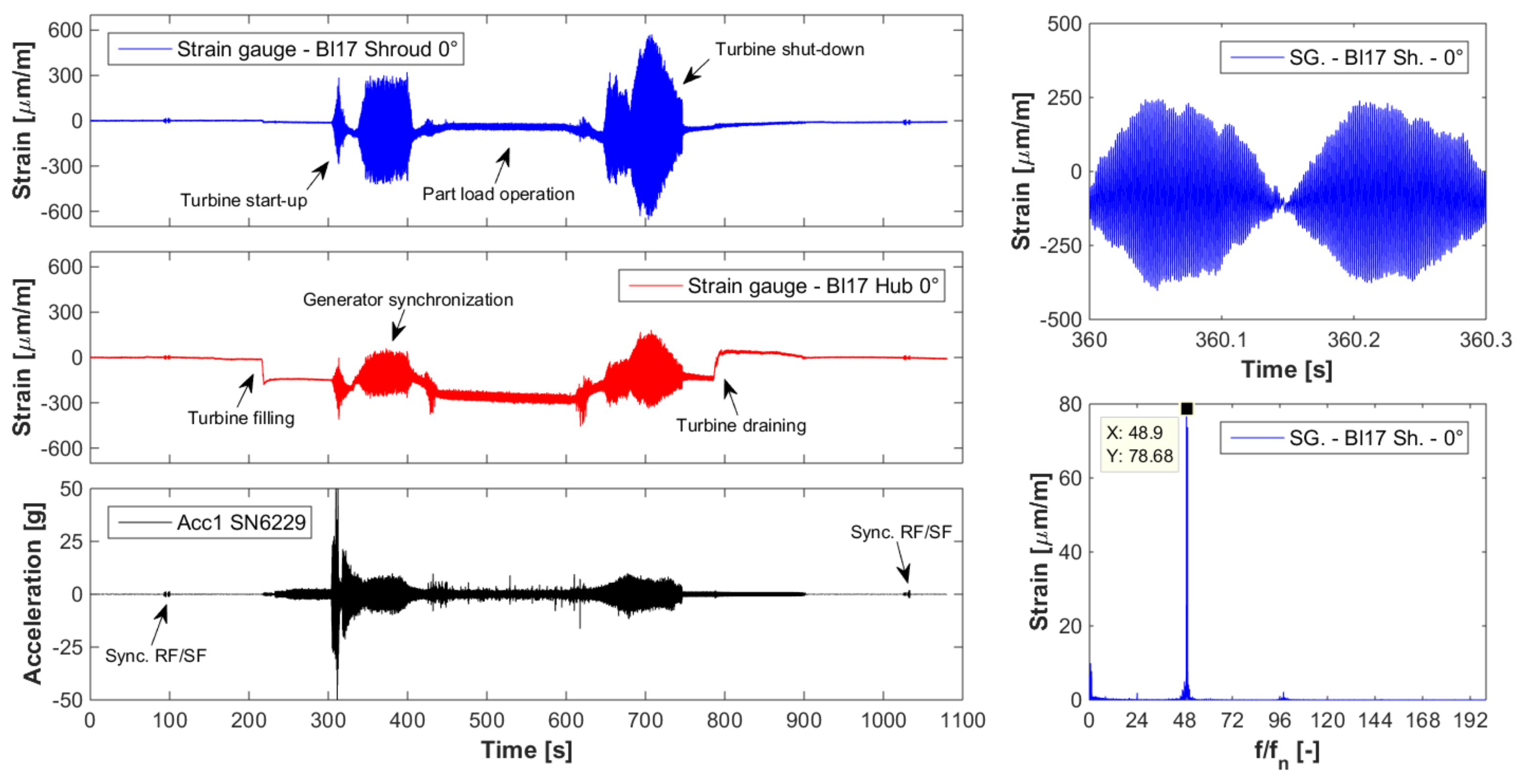
As the electricity market requires more and more flexibility, the number of start-up, stand-by, and shut-down procedures per year has increased strongly during the last decade. Consequently, the turbine spends more and more time at operating points for which the hydraulic conditions are far from the ones at the BEP. After several operation cycles, some cracks have been observed on the runner at the junction between the trailing edge of the blades and the hub. The phenomenon responsible for the development of the cracks is not yet clearly identified. However, experimental measurements on the prototype showed that the maximum amplitude of strain occurs at the SNL operating point during the synchronization of the generator with the electrical network, as well as during the shutdown phase (see Figure 1). The frequency associated with this phenomenon is close to 49$\ast f_n$ (with $f_n$ the runner frequency).

3. CFD Setup

3.1. Governing Equations

The incompressible flow is modeled by the URANS equations that are expressed in Cartesian coordinates as follows:

$$\begin{array}{cc}\hfill \frac{\partial {\overline{u}}_j}{\partial x_j}=& 0\hfill \end{array}$$

(2)

$$\begin{array}{cc}\hfill \frac{\partial \rho {\overline{u}}_i}{\partial t}+\frac{\partial \rho {\overline{u}}_j{\overline{u}}_i}{\partial x_j}=& -\frac{\partial \overline{p}}{\partial x_i}+\frac{\partial {\sigma }_{ij}}{\partial x_j}+\frac{\partial {\tau }_{ij}}{\partial x_j}\hfill \end{array}$$

(3)

with:

• $\rho$ the fluid density.
• $\overline{p}$ the mean pressure.
• ${\overline{u}}_i$ the mean velocity vector.
• ${\sigma }_{ij}$ the viscous stress tensor computed using a Newtonian linear constitutive equation.
• ${\tau }_{ij}=-\rho \overline{u_i^{{}^{\prime }}{u}_j^{{}^{\prime }}}$ the Reynolds stress tensor (an instantaneous variable a is decomposed following the Reynolds decomposition in a mean part $\overline{a}$ and a fluctuating part $a^{{}^{\prime }}$).

Two types of closure models are considered to compute the Reynolds stress tensor: models based on Boussinesq’s assumption and models based on an explicit algebraic formulation.

Boussinesq’s assumption considers a closure formulation of the Reynolds stress tensor (see Equation (4)) by analogy with the Newtonian linear constitutive equation. This assumption reduces the six unknown components of the Reynolds stress tensor to one scalar ${\mu }_t$, classically called the eddy viscosity. In order to compute the eddy viscosity, various approaches based on an algebraic formulation or one- or two-equation models have been developed [41].

$${\tau }_{ij}={\mu }_t\left(\frac{\partial u_i}{\partial x_j}+\frac{\partial u_j}{\partial x_i}\right)-\frac{2}{3}\rho k{\delta }_{ij}$$

(4)

The explicit algebraic models require formulating the Reynolds stresses as a function of the anisotropy tensor $a_{ij}$ (see Equation (5)). In the general 3D case, the anisotropy tensor can be expressed as the combination of ten tensors and five invariants [42].

$$\overline{u_i{u}_j}=k\left(a_{ij}+\frac{2}{3}{\delta }_{ij}\right)$$

(5)

In the present paper, three models based on Boussinesq’s assumption have been considered. Each of them requires solving two additional equations in order to compute the eddy viscosity. The first one is the SST $k-\omega$ model proposed by Menter [43]. This model solved a transport equation for the turbulent kinetic energy k (Equation (6)) and a transport equation for the turbulent eddy frequency $\omega$ (Equation (7)), which is in fact a blending between the $\omega$- and $ϵ$-equations (in order to limit the paper length, the values of the coefficients used in the turbulence models are not given in the paper, except the case when the value differs from the standard one. The readers are kindly requested to refer to the cited papers.).

$$\begin{array}{cc}\hfill \frac{\partial \rho k}{\partial t}+\frac{\partial \rho k{u}_j}{\partial x_j}=& P_k-{\beta }^{\ast }\rho k\omega +\frac{\partial }{\partial x_j}\left[\left(\mu +{\sigma }_k{\mu }_t\right)\frac{\partial k}{\partial x_j}\right]\hfill \end{array}$$

(6)

$$\begin{array}{cc}\hfill \frac{\partial \rho \omega }{\partial t}+\frac{\partial \rho \omega u_j}{\partial x_j}=& \frac{\alpha }{{\nu }_t}{P}_k-\beta \rho {\omega }^2+\frac{\partial }{\partial x_j}\left[\left(\mu +{\sigma }_{\omega }{\mu }_t\right)\frac{\partial \omega }{\partial x_j}\right]+2\left(1-F_1\right)\frac{\rho {\sigma }_{\omega 2}}{\omega }\frac{\partial k}{\partial x_j}\frac{\partial \omega }{\partial x_j}\hfill \end{array}$$

(7)

The eddy viscosity is then computed as:

$${\mu }_t=\frac{\rho a_{1}k}{max\left(a_1\omega ,S{F}_2\right)}$$

(8)

The formulation of the SST model can include:

• A production limiter for the turbulence production term $P_k$ (see Equation (9)), which avoids the build-up of turbulent kinetic energy in stagnation regions [44].

  $${\tilde{P}}_k=min\left(P_k,10{\beta }^{\ast }\rho k\omega \right)$$

  (9)
• A rotation-curvature correction term, which allows the model to be sensitive to streamline curvature and system rotation [45].

For ten years, an advanced formulation of the SST model has been developed by Menter and Egorov [30,46,47]. This advanced formulation, named Scale-Adaptive Simulation (SAS), is based on a revisited version of the $k-kl$ model of Rotta [48], which makes an additional production term $Q_{SAS}$ (see Equation (10)) appear in the transport equation of $\omega$ (see Equation (7)). This term makes the von Karman length scale $L_{vK}$ appear, which allows the model to adjust to the already resolved scales in the flow field.

$$Q_{SAS}=max\left[\rho {\xi }_2{S}^2{\left(\frac{L}{L_{vK}}\right)}^2-C_{SAS}\frac{2\rho k}{{\sigma }_{\mathsf{\Phi }}}max\left(\frac{1}{k^2}\frac{\partial k}{\partial x_j}\frac{\partial k}{\partial x_j},\frac{1}{{\omega }^2}\frac{\partial \omega }{\partial x_j}\frac{\partial \omega }{\partial x_j}\right),0\right]$$

(10)

with ${\xi }_2=3.51$, $C_{SAS}=2$, and ${\sigma }_{\mathsf{\Phi }}=2/3$.

For non-equilibrium turbulent flow with massive separations, the group of M. Braza have reconsidered the value of the coefficient $C_{\mu }$ in the formulation of two-equation isotropic eddy-viscosity models [49,50] and anisotropic eddy-viscosity models [51]. They have shown that the value of the coefficient $C_{\mu }=0.09$ derived from an equilibrium assumption is overestimated for unsteady detached flow. They proposed in the framework of the OES models a value of $C_{\mu }=0.02$. In the present work, the OES modeling is applied by changing the value of the coefficient ${\beta }^{\ast }$ (which corresponds to the coefficient $C_{\mu }$ in the $k-ϵ$ two-equation model formulation) from 0.09 to 0.02.

The EARSM model used in the present paper is the one developed by Wallin [52] and adjusted to the BSL $k-\omega$ model [53]. The differences are the use of a value of 1.245 for $A_1$ instead of 1.2, the neglect of the fourth order tensor polynomial contribution ${\beta }_9$, the change of the tensor basis according to [54], and the use of the standard eddy viscosity instead of the effective eddy viscosity to compute the diffusion term in the k and $\omega$ transport equations. Furthermore, the correction of the diffusion term is not used in the present calculation.

For all the models considered in the study, a wall law is used to compute the turbulent stresses in the first cell [55].

3.2. Mesh

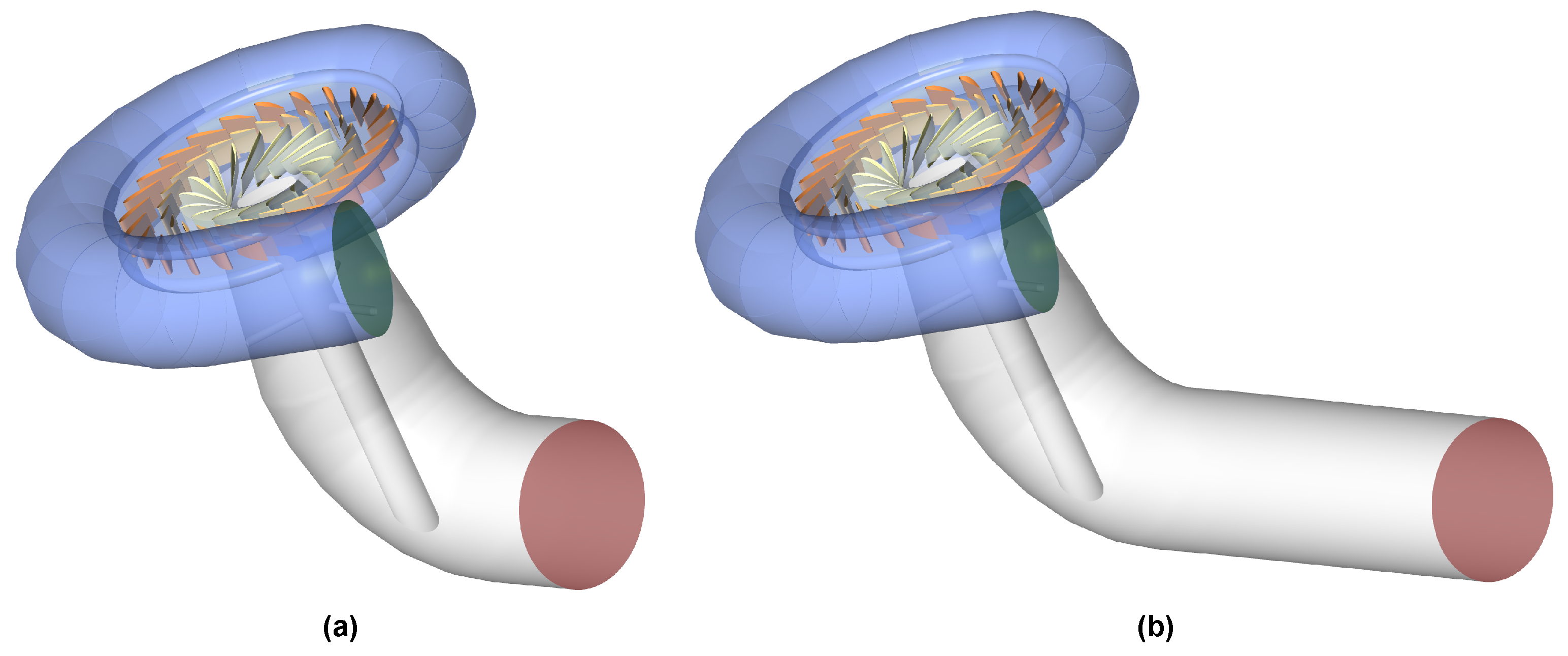
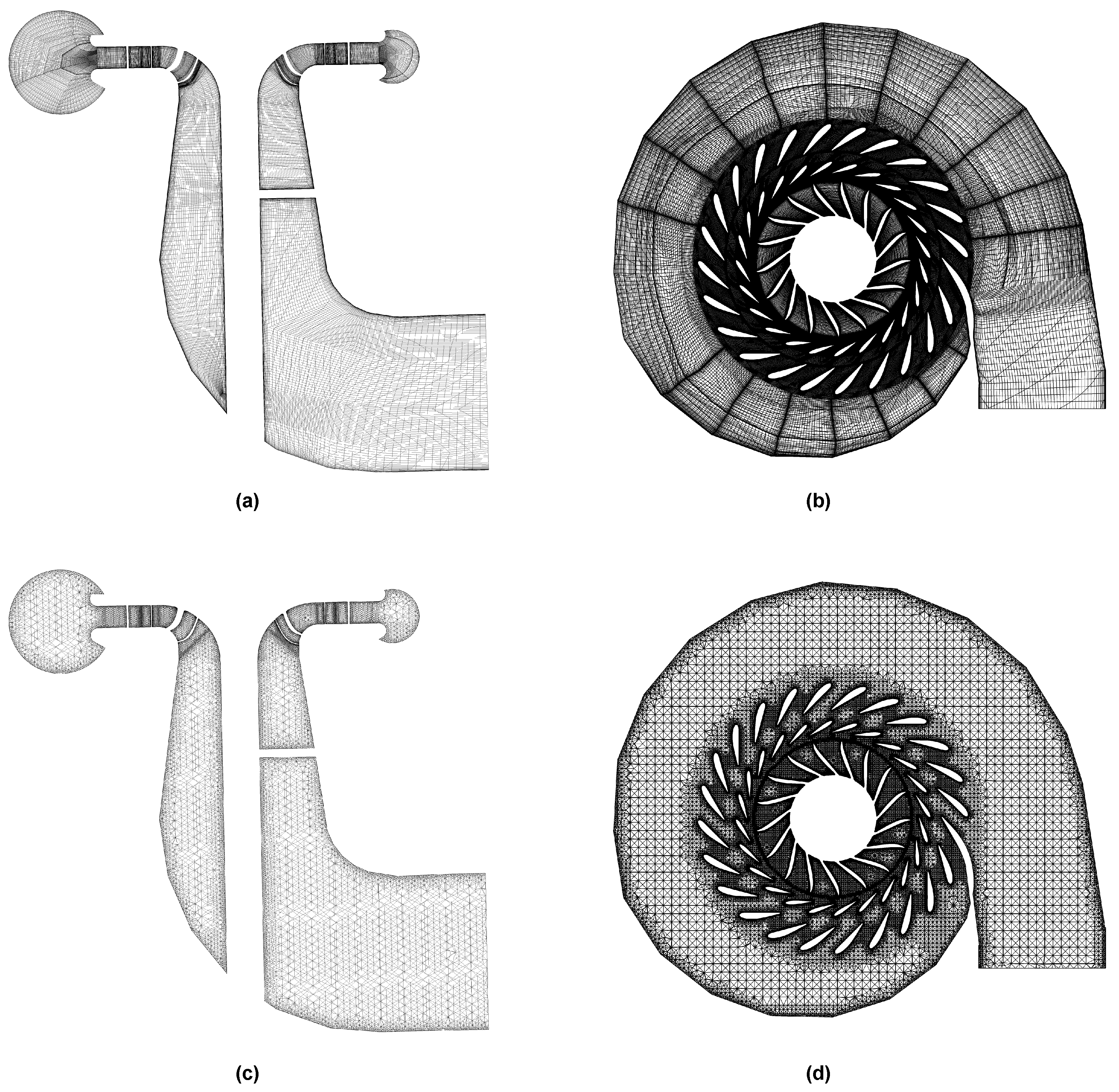
Two computational domains have been considered taking into account the whole turbine from the spiral case to the standard draft tube (see Figure 2 on the left) or an artificially-extended draft tube (see Figure 2 on the right). Two types of mesh have been considered: two structured hexahedral meshes (see Figure 3 at the top) and one unstructured mesh (see Figure 3 at the bottom) with tetrahedral and prism elements. All the meshes have been built with the ICEM CFD v17.2 software [53]. Considering the hexahedral meshes, five sub-domains are meshed separately using a blocking method. These five sub-domains are the spiral case, the stay vanes, the guide vanes, the runner, and the draft tube. The two structured meshes differ only by the height of the first cell layer at the walls in the guide vanes, runner, and draft tube domains. On the contrary, for the unstructured mesh, the whole turbine is meshed including only three fluid domains and two internal interfaces: one between the guide vanes and the runner and another between the runner and the draft tube, in order to delimit the fixed and the rotating part of the computational domain. Along the solid walls, five prism layers are generated to better resolve the boundary layer. The number of nodes and elements for each mesh are shown in

Table 1. Number of nodes and elements for each mesh.

Sub-Domain	Structured Mesh		Unstructured Mesh
	Nodes (${10}^6$)	Elements (${10}^6$)	Nodes (${10}^6$)	Elements (${10}^6$)
Spiral Case	3.7	3.6
Stay Vanes	2.9	2.8	2.8	8.9
Guide Vanes	3.7	3.5
Runner	2.8	2.6	2.2	6.6
Draft Tube	1.6	1.5	0.8	2.7
Total	14.7	14.0	5.8	18.2

. The minimum angle and the maximum aspect ratio for each mesh and each sub-domain are provided in

Table 2. Minimum angle and aspect ratio for each mesh.

Sub-Domain	Structured Mesh		Refined Structured Mesh		Unstructured Mesh
	Min Angle	Max Aspect	Min Angle	Max Aspect	Min Angle	Max Aspect
	(deg)	Ratio	(deg)	Ratio	(deg)	Ratio
Spiral Case	20	2248	20	2248
Stay Vanes	29	77	29	77	12	592
Guide Vanes	23	62	23	118
Runner	7	75	3	212	30	147
Draft Tube	20	171	20	774	20	329

. For the structured meshes, the minimum angle in the runner domain is low compared to the recommended value of 20 degrees; however, the percentage of the mesh with a poor minimum angle represents less than 1% of the runner mesh. The average $y^{+}$ on several solid walls for the BEP is given in

Table 3. Average $y^{+}$ value on solid walls. Best Efficiency Point (BEP).

Sub-Domain	Structured Mesh	Refined Structured Mesh	Unstructured Mesh
Spiral Case	720	720	90
Stay Vanes	550	550	160
Guide Vanes	850	285	300
Runner	2700	690	250
Draft Tube	330	310	90

. It is obvious that the $y^{+}$ in the runner for the structured mesh is high compared to some standard requirements. This point will be further discussed in the Results Section.

3.3. Numerical Setup

The flow inside the turbine is computed using the Ansys^® CFX v17.2 software [53]. The CFX solver uses an element-based finite volume method with a co-located grid. The Rhie–Chow discretization is used for the pressure-velocity coupling [56]. The system of equations is solved using a coupled formulation and a multigrid accelerated Incomplete Lower Upper (ILU) factorization technique. For the steady state simulations, a pseudo-time step is used to reach convergence, whereas for the unsteady simulations, the second order backward Euler scheme has been chosen. Regarding the convection terms, a high order scheme [57] is used for the mean transport equation and a first order scheme for the turbulence transport equations, except for the simulations with the SAS SST $k-\omega$ model, for which a high order scheme is specified. The fluxes at the interfaces between the stationary and rotating domains are computed using a General Grid Interface (GGI) algorithm. A frozen formulation is used for the steady simulations, whereas a fully-transient approach is used for the unsteady simulations.

Regarding the boundary conditions:

• no-slip walls are specified at the solid walls.
• the mass flow rate or the total pressure is set at the inlet of the spiral case.
• the surface averaged pressure is set at the outlet through an opening boundary condition.
• the rotational speed is imposed in the rotating domain.

4. BEP Results

The simulations at the BEP aim at checking and validating the CFD setup using only the SST $k-\omega$ turbulence model. Several simulations (see

Table 4. List of the computations performed at the BEP.

Reference	Algorithm	Rotor/Stator Interface	Computational Domain	Mesh	Inlet Boundary Condition
CFD1	Steady	Frozen	standard	structured	mass flow rate
CFD2	Steady	Frozen	standard	refined structured	mass flow rate
CFD3	Steady	Frozen	standard	unstructured	mass flow rate
CFD4	Steady	Frozen	extended	structured	mass flow rate
CFD5	Steady	Frozen	standard	structured	total pressure
CFD6	Unsteady	Transient	standard	structured	mass flow rate

) have been performed in order to investigate the influence of the mesh, the size of the computational domain, the algorithm, and the inlet boundary conditions. Regarding the unsteady simulation CFD6, the time step was set to a 0.9${}^{\circ }$ revolution per time step, and three runner revolutions have been computed.

The results compare the discharge $Q_{ED}$, the speed $n_{ED}$, and power $P_{ED}$ factors and the dimensionless efficiency (the dimensionless efficiency was computed as the ratio between the CFD and measured efficiencies) ${\eta }^{\ast }$ with the measured values (see

Table 5. CFD results at the BEP compared with the measurements.

Reference	${\mathit{Q}}_{\mathit{E}\mathit{D}}$	${\mathit{n}}_{\mathit{E}\mathit{D}}$	${\mathit{P}}_{\mathit{E}\mathit{D}}$	${\mathit{\eta }}^{\ast }$
CFD1	0.187	0.268	0.175	1.00
CFD2	0.190	0.271	0.177	1.00
CFD3	0.188	0.269	0.177	1.01
CFD4	0.187	0.267	0.174	0.99
CFD5	0.186	0.275	0.174	1.00
CFD6	0.187	0.268	0.178	1.01
EXP	0.183	0.271	0.171	1.00

). Regarding the discharge factor $Q_{ED}$, the discrepancy between the CFD and the measurements was between +1.4% for the computation CFD5 with the imposed total pressure at the inlet and +3.8% for the computation CFD2 using the refined structured mesh. For the speed factor $n_{ED}$, the discrepancy was between −1.5% for the computation CFD4 with the extended draft tube and +1.5% for the computation CFD5 with the imposed total pressure at the inlet. The power factor $P_{ED}$ was overestimated at least by +1.8% and at most by +4%. Finally, the dimensionless efficiency was predicted with 1% of precision. Keeping in mind the uncertainties on the input and measured values and the fact that the leakage flow through the labyrinths is neglected in the CFD, the accuracy of the numerical results was good and not strongly influenced by the numerical setup or the mesh.

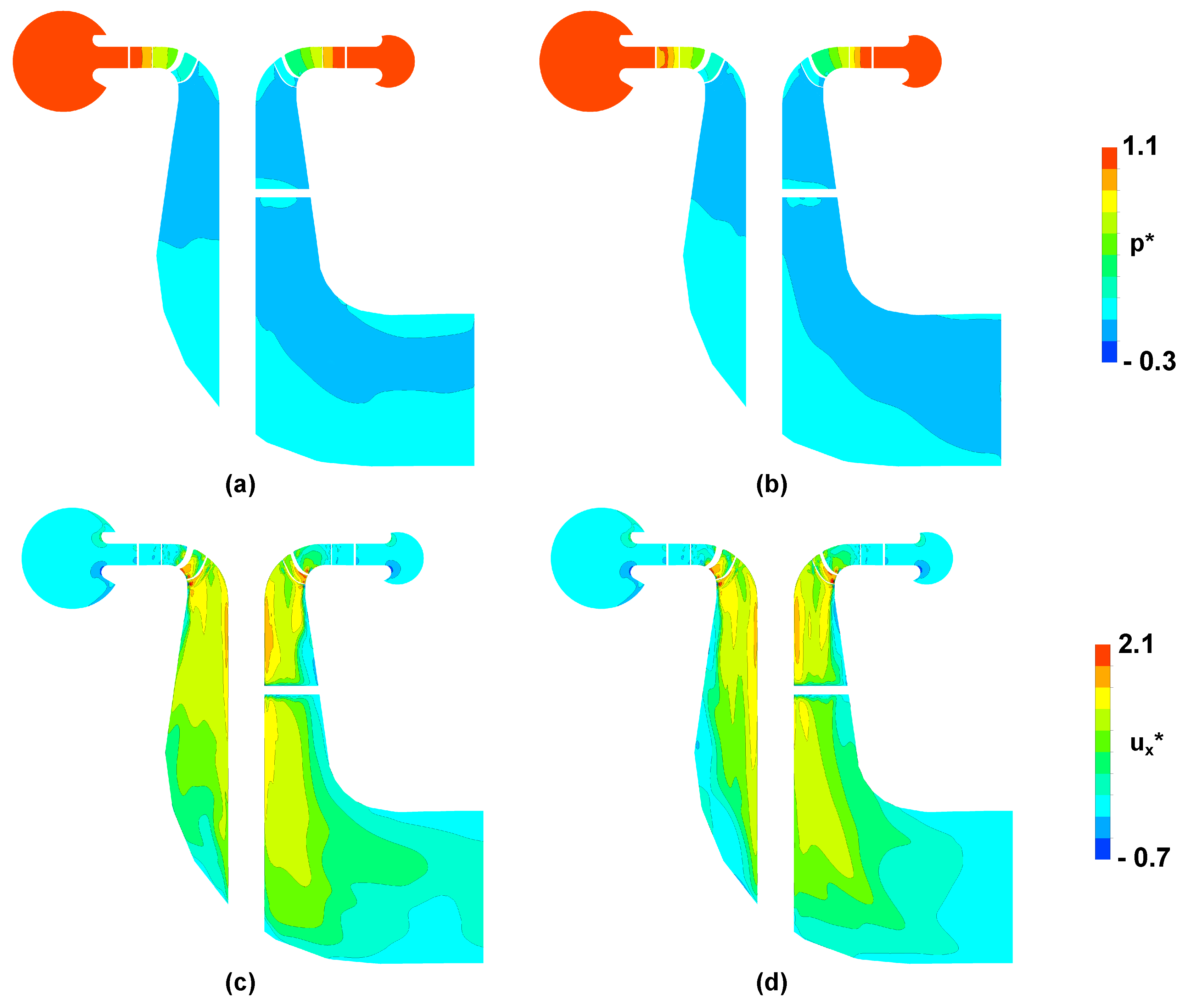
Figure 4 shows the dimensionless pressure and axial velocity contours in the meridional plane provided by the simulations CFD1 (structured mesh) and CFD2 (refined structured mesh). No differences were observed on the pressure contours between the two meshes. Regarding the axial velocity contours, both simulations gave the same pattern, with spots of high magnitude at the trailing edge of the runner blades close to the shroud. The small differences in the draft tube cone can be related to the use of a frozen interface.

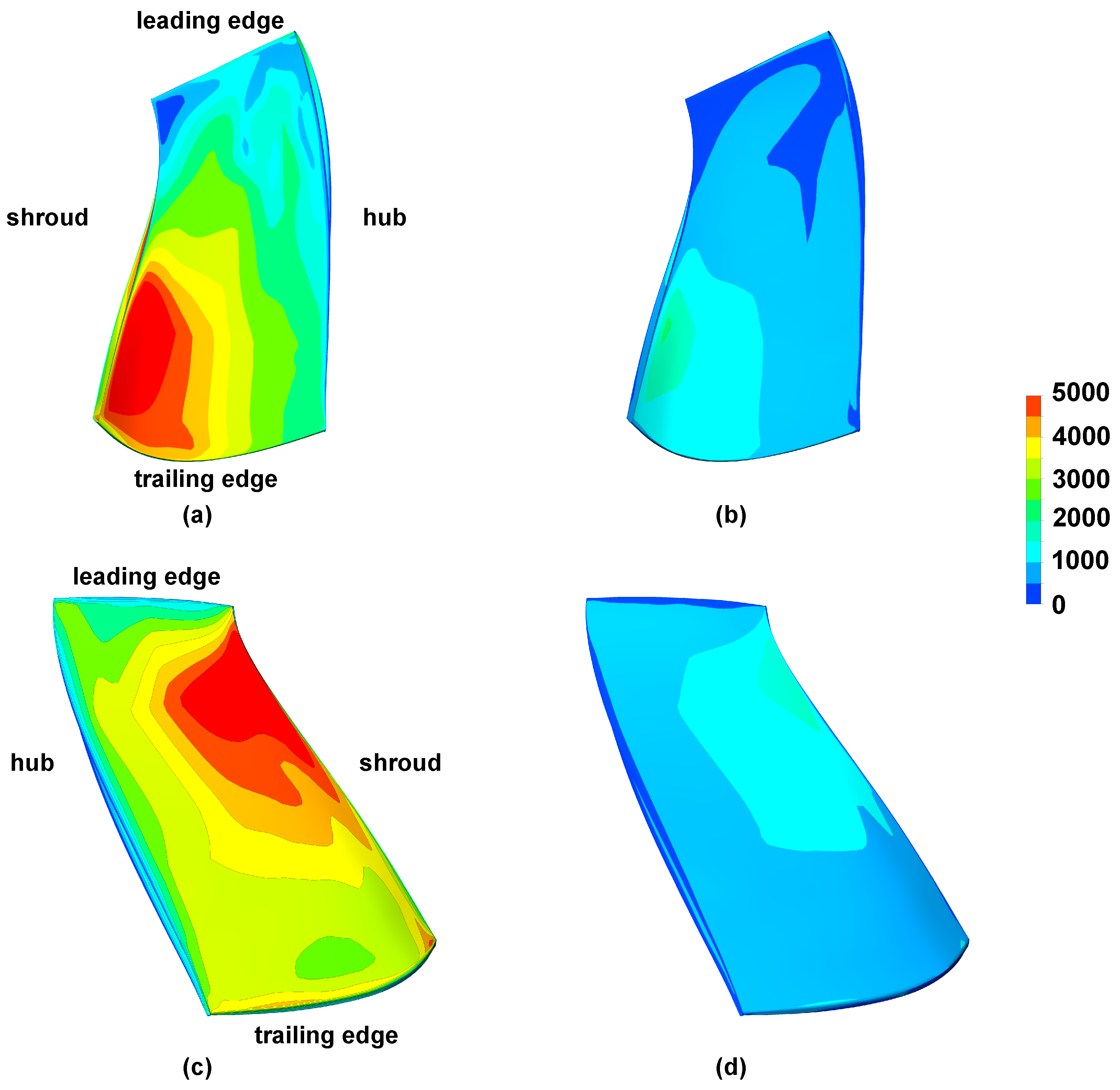
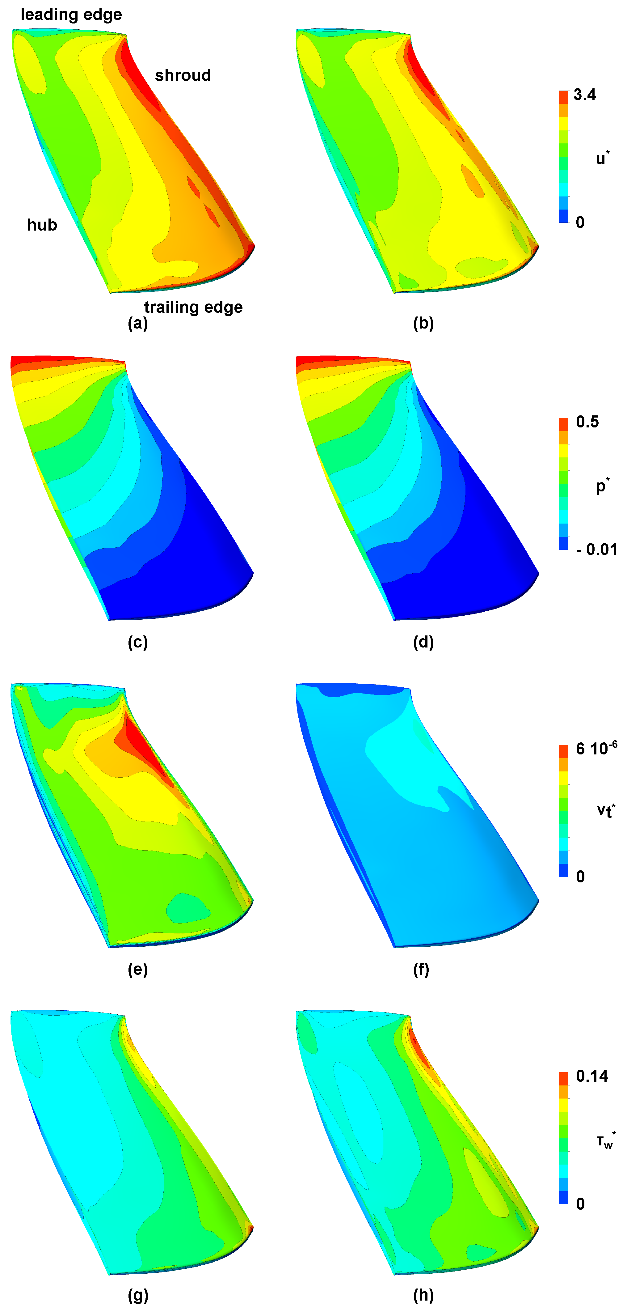
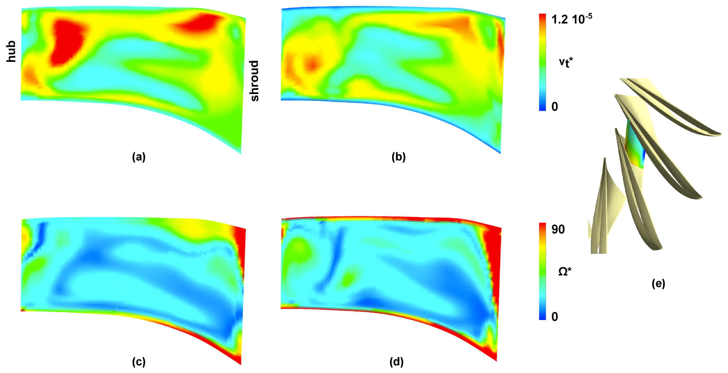
The $y^{+}$ contours on one of the blades are displayed in Figure 5 for both simulations CFD1 and CFD2. The refined mesh led to a reduction of the $y^{+}$ by a factor of three. The $y^{+}$ were very high in two regions: one on the pressure side at the trailing edge close to the shroud and one on the suction side at the leading edge close to the shroud. In order to investigate the influence of the $y^{+}$ values on the flow in the turbine, the contours of the dimensionless magnitude of the relative velocity, pressure, eddy viscosity, and wall shear stress on the suction side of one blade are shown in Figure 6 for both meshes. For each quantity, the pattern of the contours was the same. The differences between the two meshes were observed mainly for the dimensionless eddy viscosity, which is lower on the refined mesh, as expected. The wall shear stress was slightly higher on the refined mesh at the shroud close to the leading edge. The relative velocity differed along the shroud with a lower value predicted by the refined mesh, which is in agreement with the refinement of the mesh at the walls. Finally, the contours of the dimensionless magnitude of the vorticity and eddy viscosity in a cross-section of a blade channel are displayed in Figure 7. The pattern for the two quantities was rather the same for the two meshes, even if close to the hub, the simulation CFD1 made a region with a low magnitude of the vorticity appear, which is not observed on the refined mesh (simulation CFD2).

From the above analysis of the flow, it can be concluded that the simulation CFD1, with a slightly coarse mesh at the walls, allowed capturing the main features of the flow with an acceptable accuracy. Consequently, this mesh was used for the computations at the SNL operating point.

5. SNL Results

The SNL operating point was computed using the different turbulence models described in the governing equations subsection. The procedure for the computations was as follows: first, the SST model was used to compute a steady state simulation, then 6.25 runner revolutions with a time step set to 0.9${}^{\circ }$ of revolution per time step were computed, and finally, 6.25 additional runner revolutions with a time step reduced to 0.36${}^{\circ }$ of revolution per time step were computed. This last result was used as an initial guess to compute 6.25 additional runner revolutions simulated using: the SST model with the activation of the Curvature Correction and the Production limiter (SST-CC-Plim), the SST-OES model with a value of ${\beta }^{\ast }=0.02$, the SST-SAS model, and the BSL-EARSM model. The CPU time required for 6.25 runner revolutions was around $5\times {10}^7$ s, which corresponds to approximately one month on 24 CPUs.

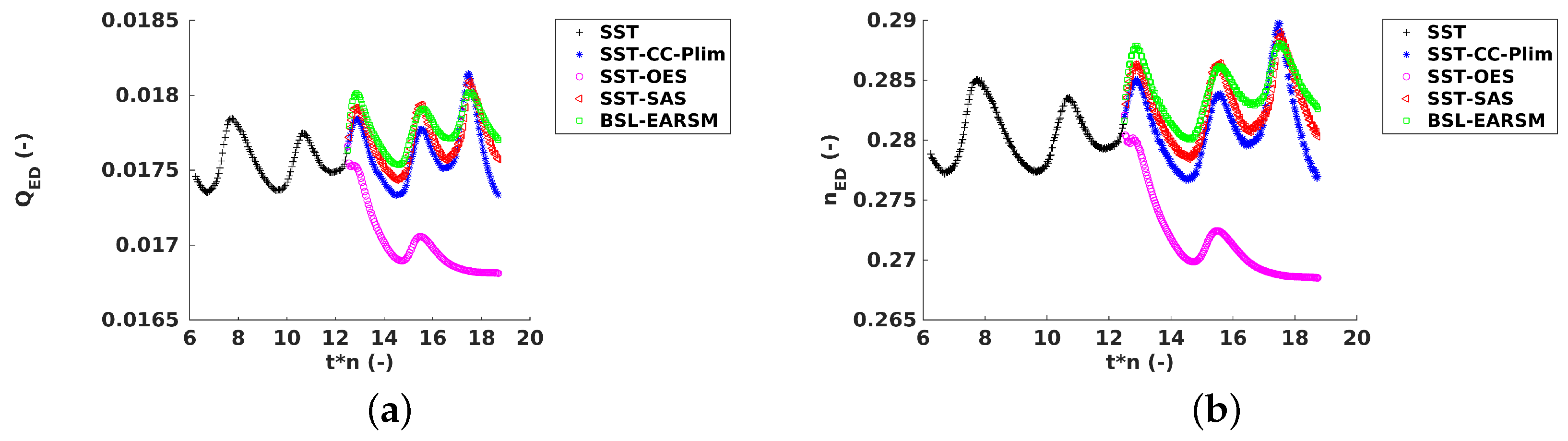
The time history of the discharge and speed factors are displayed in Figure 8. A low frequency was observed on both factors for each turbulence model except for the SST-OES model, which seemed to converge to a stable operating point. The four other turbulence models presented a similar time evolution of the global parameters of the turbine. The time-averaged values of the $Q_{ED}$ and $n_{ED}$ over 6.25 runner revolutions are given in

Table 6. CFD results at the SNL operating point compared with the measurements. Averaged values over 6.25 runner revolutions.

Turbulence Model	${\mathit{Q}}_{\mathit{E}\mathit{D}}$	${\mathit{n}}_{\mathit{E}\mathit{D}}$
SST	0.0176	0.280
SST-CC-Plim	0.0176	0.281
SST-OES	0.0170	0.272
SST-SAS	0.0177	0.283
BSL-EARSM	0.0178	0.284
EXP	0.0170	0.270

for each simulation. However, for the SST-OES model, the final values of the $Q_{ED}=0.0168$ and $n_{ED}=0.269$ were more valuable. Comparing with the experimental data, the SST-OES model was the one that provided the closest values of the $Q_{ED}$ and $n_{ED}$ within an accuracy of 1%. The others turbulence models overestimated the $Q_{ED}$ and $n_{ED}$, whereas, for the BSL-EARSM model, a maximum overestimation of the $Q_{ED}$ value by 4.7% and of the $n_{ED}$ value by 5.2%.

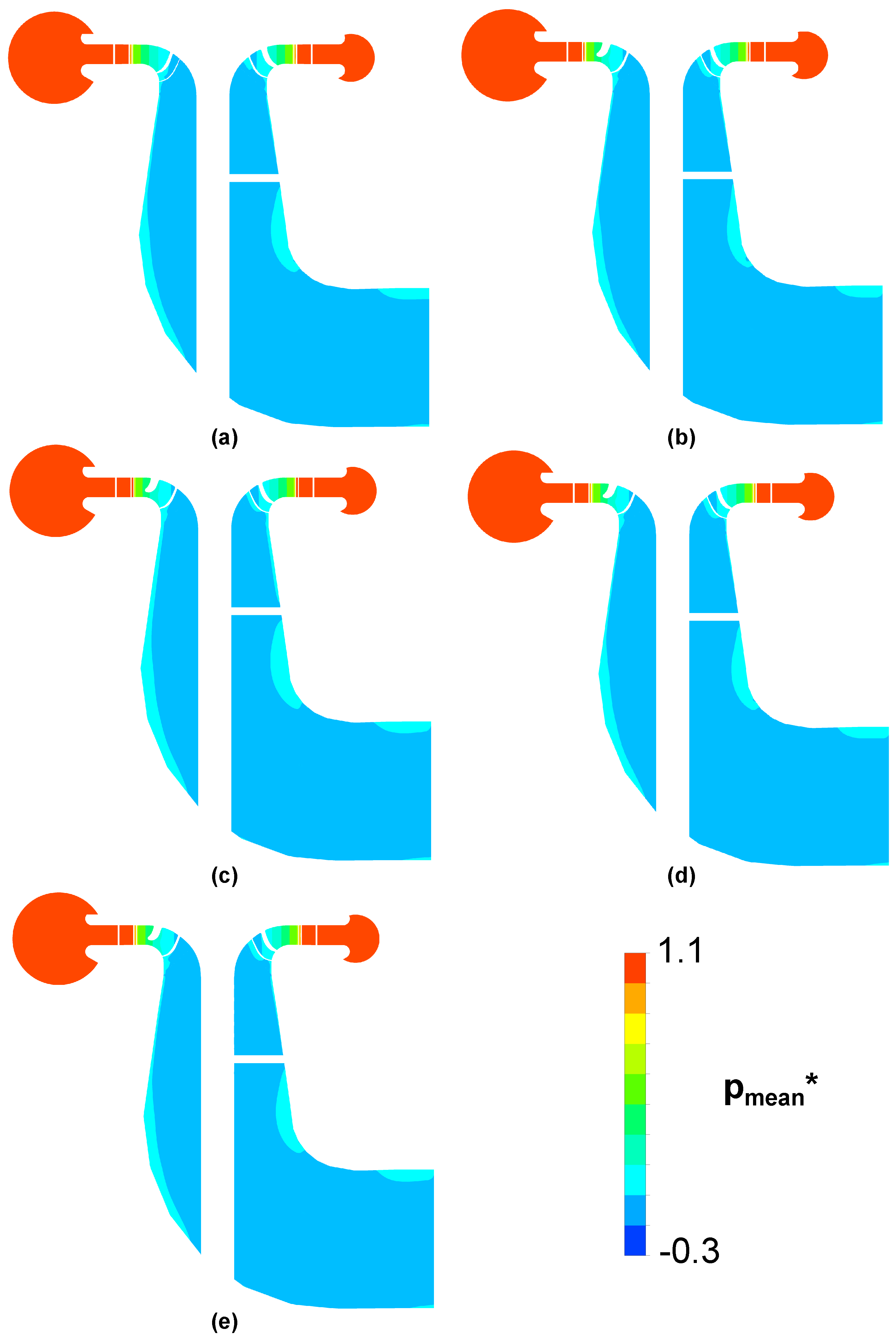
The contours of the dimensionless axial velocity (Figure 9) and pressure (Figure 10) on the meridional plane did not show any difference between the turbulence models. Comparing to the BEP, the pressure field was not strongly affected, whereas the axial flow was mainly concentrated close to the wall of the draft tube with a recirculation in the center of the draft tube around the tripod.

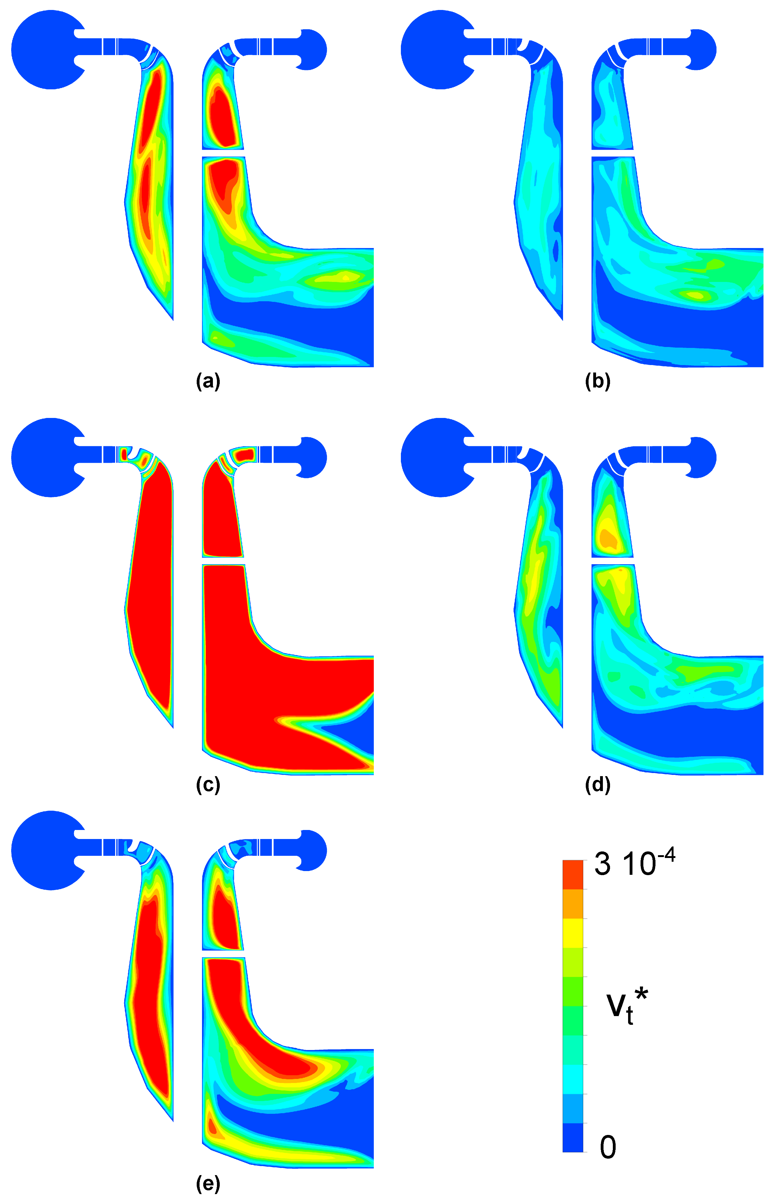
Despite the weak influence of the turbulence model on the mean pressure and axial velocity, the turbulence field was strongly affected by the turbulence model, as shown in Figure 11, which displays the instantaneous contours of the dimensionless eddy viscosity on the meridional plane. Compared to the SST model, the BSL-EARSM and the SST-OES models led to an increase of the eddy viscosity in the runner and the draft tube, whereas the SST-CC-Plim and the SST-SAS models led to a decrease of the eddy viscosity. The large magnitude of the eddy viscosity predicted by the SST-OES model was the explanation for the stable behavior observed on the $Q_{ED}$ and $n_{ED}$ factors.

The instantaneous iso-surface of the Q-criterion in the runner (downstream view) is shown on Figure 12. The SST model predicted a large spanwise vortex close to the trailing edge of the runner blade. Downstream of the vortex, a high pressure region was observed. The vortex was stable in time and identical in each blade channel. The SST-CC-Plim and BSL-EARSM models provided the same pattern, but the vortex was less expanded in the spanwise direction. Moreover, some small vortex shedding was observed with the SST-CC-Plim model. Regarding the SST-OES model, no vortices were present, and the high pressure region disappeared. Finally, the SST-SAS model provided a more chaotic pattern of vortices in the blade channel, with still the presence of a high pressure region in the vicinity of the hub and the blade trailing edge.

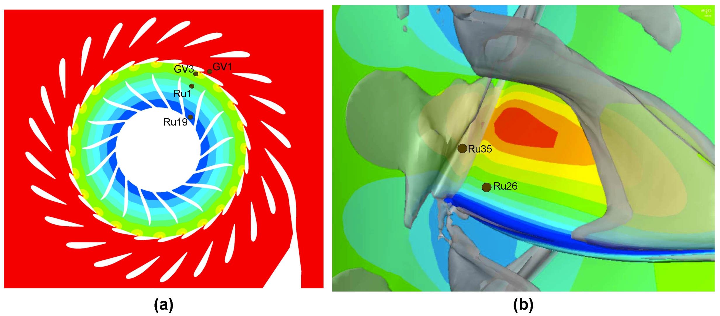
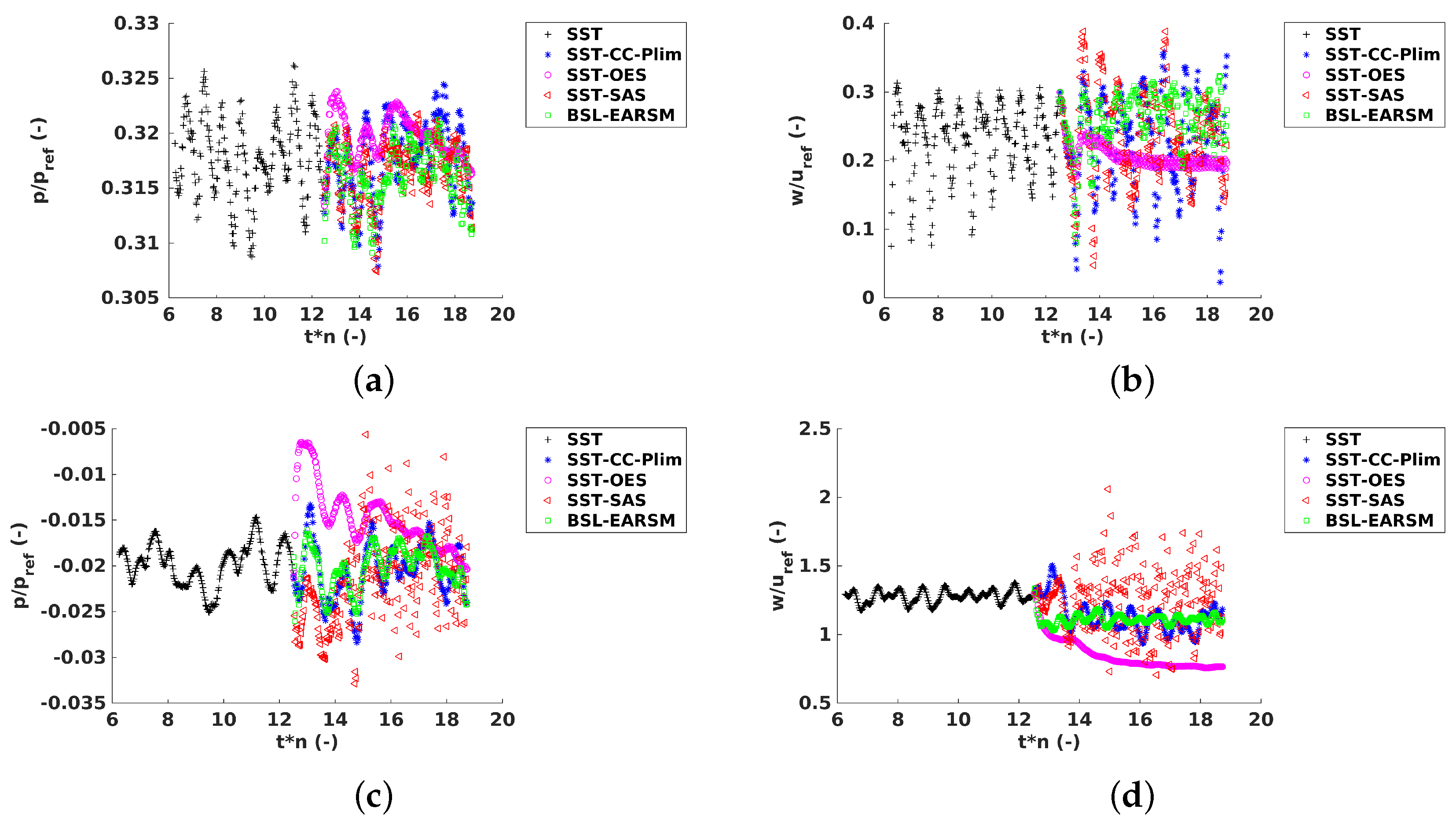
Several probes have been located in one guide vane and blade channel (see Figure 13). The probe GV1 was located upstream of the passage reduction due to the low opening of the guide vanes, whereas the probe GV3 was located just downstream of the passage reduction. The probes Ru1 and Ru19 were located in the middle of the blade channel, whereas the probes Ru26 (close to the trailing edge of the blade) and Ru35 (close to the hub) were located on the suction side downstream of the large spanwise vortex described previously.

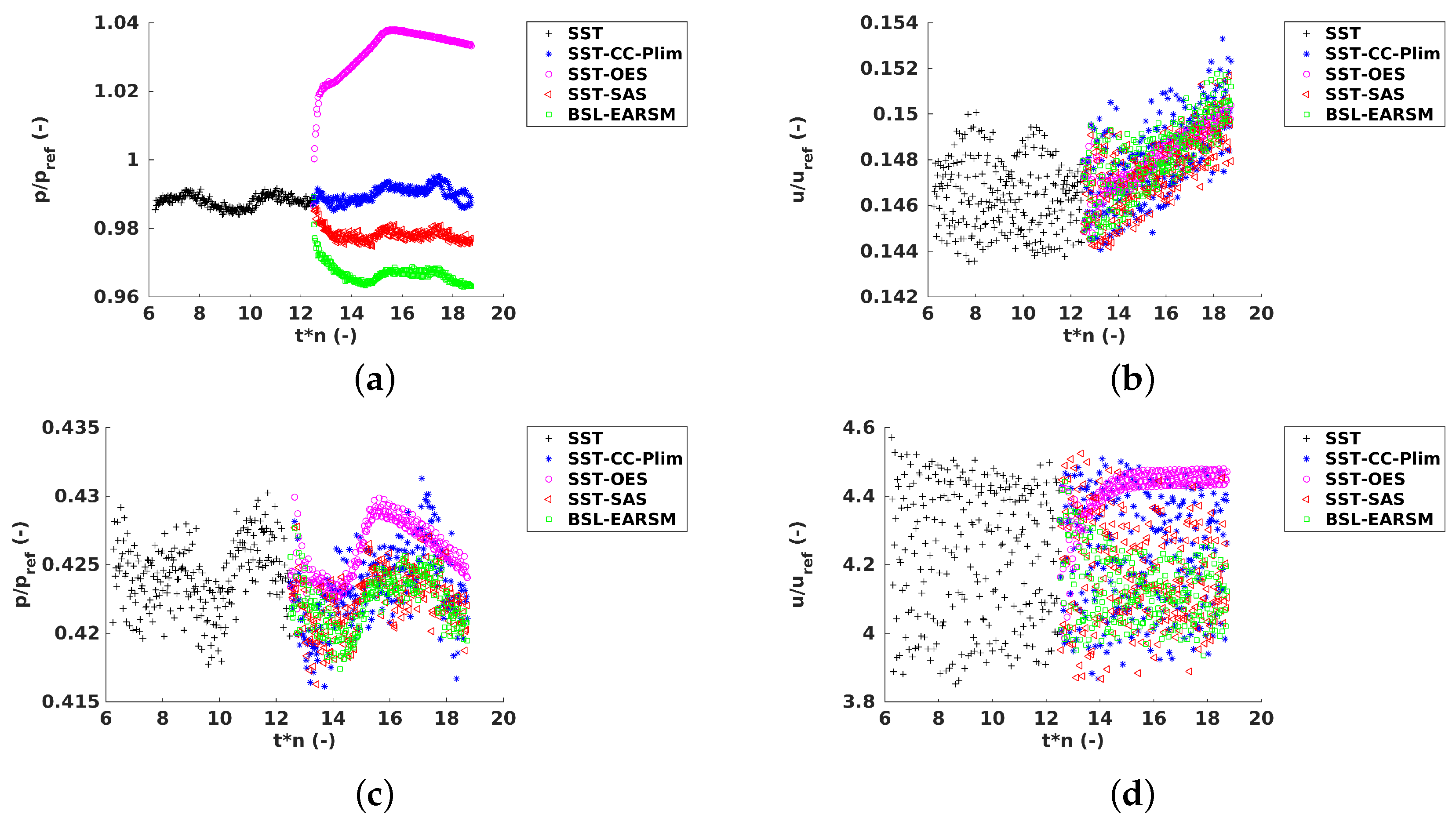
The time history of the dimensionless pressure and velocity magnitude in the guide vane channel is shown on Figure 14. At position GV1, the turbulence model influenced the pressure level, which was higher for the SST-OES model and lower for the SST-SAS and BSL-EARSM models compared with the SST model. The SST-CC-Plim model did not change the pressure level compared to the SST model. At position GV3, the pressure level was the same for all the models, even if the fluctuations were damped by the SST-OES model. Therefore, the pressure drop at the guide vane passage differed between the different models, explaining the differences in the predicted speed and discharge factors. Indeed, since the SST-OES model predicted a higher pressure drop at the guide vanes, then the predicted specific energy was higher, and the speed and discharge factors were lower. Regarding the velocity magnitude, at position GV1, all the models provided the same behavior characterized by a positive slope compared to the SST model. This feature was absent at position GV3, where large velocity fluctuations were observed compared to position GV1, except for the SST-OES model.

In the runner blade channel (see Figure 15), at location Ru1, the models predicted more or less the same dynamics, except the SST-OES model, which damped the pressure and velocity fluctuations. This feature was more pronounced downstream at the locations Ru19. At this position, the SST-SAS showed larger fluctuations than the others turbulence models.

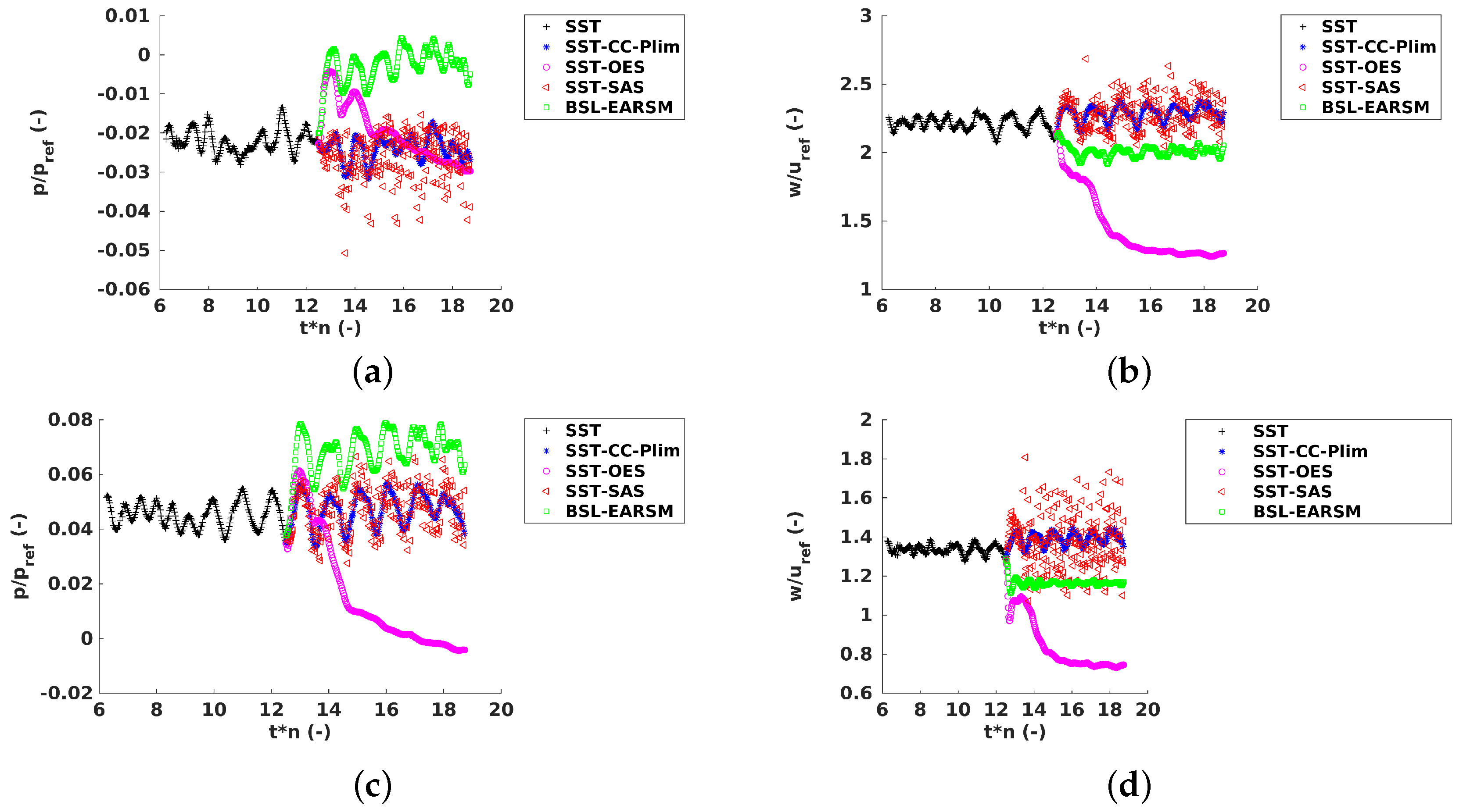
Finally, at locations Ru26 and Ru35 (see Figure 16), the SST-OES once again damped the fluctuations and provided a stable signal. The SST-CC-Plim model followed the behavior of the SST model. The BSL-EARSM model presented a similar behavior, but with a shift regarding the time-averaged pressure and velocity. The SST-SAS model predicted a higher amplitude of the pressure and velocity signals.

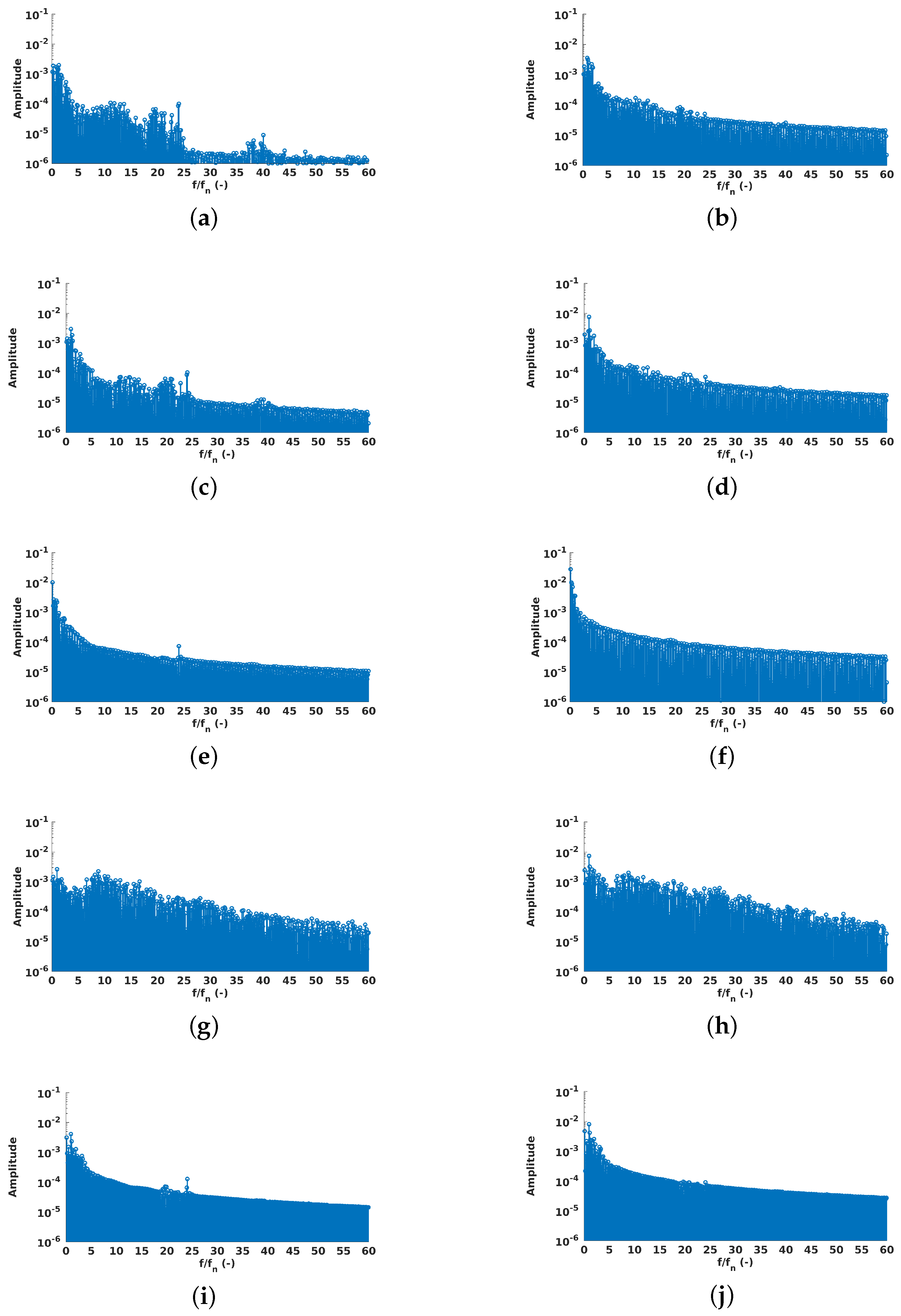
The pressure signals at the locations Ru26 and Ru35 have been transformed into the Fourier space, and the corresponding dimensionless amplitude is plotted against the scale frequency in Figure 17. At location Ru26, the SST model showed several peaks at frequencies lower than the scale frequency $f/f_n=24$, which corresponds to the guide vane passage frequency. Above this frequency, the amplitude decreased by one order of magnitude. Apart from the SST-SAS model, all the others models exhibited a peak at the scale frequency $f/f_n=24$. Beyond this frequency, the decrease in amplitude disappeared, which means that contrary to the SST model, these models increased the fluctuations at frequencies higher than the guide vane passage frequency. In the particular case of the SST-SAS model, no specific frequency was put in evidence due to the higher amplitudes predicted for all the frequencies, masking the guide vane passage frequency. At location Ru35, no specific frequency was captured by the models; however, SST-SAS still provided higher amplitudes for all the frequencies compared to the other models.

Regarding the large strain fluctuations that were observed experimentally at a scale frequency $f/f_n=49$, none of the simulations made such a frequency appear. Therefore, it seemed that the flow did not provide a specific excitation source for the structure. Nevertheless, as shown by the pressure spectrum provided by the SST-SAS model, the level of pressure fluctuations was increased around the scale frequency $f/f_n=49$ by the advanced turbulence models compared to the SST model.

6. Conclusions

The SNL operating point of a high head Francis turbine was investigated using several “advanced” RANS turbulence models. The unsteady simulations have been compared with the results obtained using the standard SST $k-\omega$ turbulence model and the available experimental data. The mean flow was slightly influenced by the turbulence model, which means that the flow pattern and the time-averaged global parameters of the turbine such as the speed or discharge factors were computed within an accuracy of less than 5%. This range of 5% was due to a difference in the pressure drop at the restriction passage imposed by the small guide vane opening. On the contrary, the turbulence field and the dynamics of the flow were strongly influenced by the turbulence models. For instance, the SST-OES model led to a quasi-stable behavior of the flow due to an increase of the eddy viscosity in the runner and the draft tube. Conversely, the SST-SAS model increased the level of pressure and velocity fluctuations compared with the standard SST model. The BSL EARSM model and the SST model with the curvature correction and production limiter shared the same behavior as the SST model, but they provided a little bit higher pressure and velocity fluctuations, mainly for frequencies beyond the guide vane passage frequency.

However, none of the models showed a specific excitation at the scale frequency $f/f_n=49$, whereas experimentally, the strain gauges exhibited a strong excitation. As this frequency could correspond to an eigenfrequency of the turbine, further investigations are required. It could be already suggested that the SST-SAS should provide a higher excitation source due to the higher pressure fluctuations predicted.

References

- Renewables 2018, Global Status Report; Renewable Energy Policy Network for the 21st Century: Paris, France, 2018.
- Paish, O. Micro-hydropower: Status and prospects. Proc. Inst. Mech. Eng. Part A J. Power Energy 2002, 216, 31–40. [Google Scholar] [CrossRef]
- Pérez-Sánchez, M.; Sánchez-Romero, F.J.; Ramos, H.M.; López-Jiménez, P.A. Energy recovery in existing water networks: Towards greater sustainability. Water 2017, 9, 97. [Google Scholar] [CrossRef]
- Spänhoff, B. Current status and future prospects of hydropower in Saxony (Germany) compared to trends in Germany, the European Union and the World. Renew. Sustain. Energy Rev. 2014, 30, 518–525. [Google Scholar] [CrossRef]
- Ibrahim, H.; Ilinca, A.; Perron, J. Energy storage systems—Characteristics and comparisons. Renew. Sustain. Energy Rev. 2008, 12, 1221–1250. [Google Scholar] [CrossRef]
- Mohd, A.; Ortjohann, E.; Schmelter, A.; Hamsic, N.; Morton, D.; Westphalia, S.; Sciences, A.; Soest, D.; Ring, L. Challenges in integrating distributed Energy storage systems into future smart grid. In Proceedings of the 2008 IEEE International Symposium on Industrial Electronics, Cambridge, UK, 30 June–2 July 2008; pp. 1627–1632. [Google Scholar] [CrossRef]
- Lowys, P.Y.; Guillaume, R.; André, F.; Duparchy, F.; Castro Ferreira, J.; Ferreira da Silva, A.; Duarte, F. Alqueva II and Salamonde II: A new approach for extending turbine operation range. In Proceedings of the Hydro 2014, Cernobbio, Italy, 13–15 October 2014. [Google Scholar]
- Keck, H.; Sick, M. Thirty years of numerical flow simulation in hydraulic turbomachines. Acta Mech. 2008, 229, 211–229. [Google Scholar] [CrossRef]
- Sick, M.; Michler, W.; Weiss, T.; Keck, H. Recent developments in the dynamic analysis. Proc. Inst. Mech Eng. Part A Power Energy 2009, 223, 415–427. [Google Scholar] [CrossRef]
- Avellan, F. Flow Investigation in a Francis Draft Tube: The Flindt Project. In Proceedings of the 20th IAHR Symposium, Charlotte, NC, USA, 6–9 August 2000; pp. 1–18. [Google Scholar]
- Flemming, F.; Foust, J.; Koutnik, J.; Fisher, R.K. Overload Surge Investigation Using CFD Data. Int. J. Fluid Mach. Syst. 2009, 2, 315–323. [Google Scholar] [CrossRef] [Green Version]
- Decaix, J.; Müller, A.; Favrel, A.; Avellan, F.; Münch, C. URANS Models for the Simulation of Full Load Pressure Surge in Francis Turbines Validated by Particle Image Velocimetry. J. Fluids Eng. 2017, 139, 121103. [Google Scholar] [CrossRef]
- Aakti, B.; Amstutz, O.; Casartelli, E.; Romanelli, G.; Mangani, L. On the performance of a high head Francis turbine at design and off-design conditions. J. Phys. Conf. Ser. 2015, 579, 012010. [Google Scholar] [CrossRef] [Green Version]
- Wack, J.; Riedelbauch, S. Numerical simulations of the cavitation phenomena in a Francis turbine at deep part load conditions. J. Phys. Conf. Ser. 2015, 656, 012074. [Google Scholar] [CrossRef] [Green Version]
- Ciocan, G.D.; Iliescu, M.S.; Vu, T.C.; Nennemann, B.; Avellan, F. Experimental Study and Numerical Simulation of the FLINDT Draft Tube Rotating Vortex. J. Fluids Eng. 2007, 129, 146–158. [Google Scholar] [CrossRef] [Green Version]
- Casartelli, E.; Mangani, L.; Romanelli, G.; Staubli, T. Transient simulation of speed-no load conditions with an open-source based C++ code. IOP Conf. Ser. Earth Environ. Sci. 2014, 22, 032029. [Google Scholar] [CrossRef]
- Nennemann, B.; Morissette, J.F.; Chamberland-Lauzon, J.; Monette, C.; Braun, O.; Melot, M.; Coutu, A.; Nicolle, J.; Giroux, A.M. Challenges in dynamic pressure and stress predictions at no-load operation in hydraulic turbines. IOP Conf. Ser. Earth Environ. Sci. 2014, 22, 032055. [Google Scholar] [CrossRef]
- Seidel, U.; Mende, C.; Hübner, B.; Weber, W.; Otto, A. Dynamic loads in Francis runners and their impact on fatigue life. IOP Conf. Ser. Earth Environ. Sci. 2014, 22, 032054. [Google Scholar] [CrossRef] [Green Version]
- Stens, C.; Riedelbauch, S. Investigation of a fast transition from pump mode to generating mode in a model scale reversible pump turbine. IOP Conf. Ser. Earth Environ. Sci. 2016, 49, 112001. [Google Scholar] [CrossRef]
- Nicolle, J.; Morissette, J.F.; Giroux, A.M. Transient CFD simulation of a Francis turbine startup. IOP Conf. Ser. Earth Environ. Sci. 2012, 15, 062014. [Google Scholar] [CrossRef] [Green Version]
- Casartelli, E.; Mangani, L.; Ryan, O.; Schmid, A. Application of transient CFD-procedures for S-shape computation in pump-turbines with and without FSI. IOP Conf. Ser. Earth Environ. Sci. 2016, 49, 042008. [Google Scholar] [CrossRef] [Green Version]
- Trivedi, C.; Cervantes, M.J.; Dahlhaug, O.G. Experimental and numerical studies of a high-head Francis turbine: A review of the Francis-99 test case. Energies 2016, 9, 74. [Google Scholar] [CrossRef]
- Trivedi, C.; Cervantes, M.J. State of the art in numerical simulation of high head Francis turbines. Renew. Energy Environ. Sustain. 2016, 1, 20. [Google Scholar] [CrossRef] [Green Version]
- Pacot, O.; Kato, C.; Guo, Y.; Yamade, Y.; Avellan, F. Large Eddy Simulation of the Rotating Stall in a Pump-Turbine Operated in Pumping Mode at a Part-Load Condition. J. Fluids Eng. 2016, 138, 111102. [Google Scholar] [CrossRef]
- Spalart, P.R.; Jou, W.H.; Strelets, M.; Allmaras, S.R. Comments on the feasibility of LES for wings and on a hybrid RANS/LES approach. In Advances in DNS/LES; Greyden Press: Ruston, LA, USA, 1997; Volume 1, pp. 137–148. [Google Scholar]
- Spalart, P.R. Detached-Eddy Simulation. Annu. Rev. Fluid Mech. 2009, 41, 181–202. [Google Scholar] [CrossRef]
- Krappel, T.; Kuhlmann, H.; Kirschner, O.; Ruprecht, A.; Riedelbauch, S. Validation of an IDDES-type turbulence model and application to a Francis pump turbine flow simulation in comparison with experimental results. Int. J. Heat Fluid Flow 2015, 55, 167–179. [Google Scholar] [CrossRef]
- Minakov, A.; Sentyabov, A.; Platonov, D.; Dekterev, A.; Gavrilov, A. Numerical modeling of flow in the Francis-99 turbine with Reynolds stress model and detached eddy simulation method. J. Phys. Conf. Ser. 2015, 579, 012004. [Google Scholar] [CrossRef] [Green Version]
- Menter, F.R.; Egorov, Y. A Scale-Adaptive Simulation Model using Two-Equation Models. In Proceedings of the 45rd AIAA Aerospace Sciences Meeting and Exhibit, Reno, NV, USA, 10–13 January 2005. [Google Scholar]
- Menter, F.; Egorov, Y. The Scale-Adaptive Simulation Method for Unsteady Turbulent Flow Predictions. Part 1: Theory and Model Description. Flow Turbul. Combust. 2010, 85, 113–138. [Google Scholar] [CrossRef]
- Neto, A.D.A.; Jester-Zuerker, R.; Jung, A.; Maiwald, M. Evaluation of a Francis turbine draft tube flow at part load using hybrid RANS-LES turbulence modeling. IOP Conf. Ser. Earth Environ. Sci. 2012, 15, 062010. [Google Scholar] [CrossRef]
- Mössinger, P.; Jester-Zürker, R.; Jung, A. Investigation of different simulation approaches on a high-head Francis turbine and comparison with model test data: Francis-99. IOP Conf. Ser. J. Phys. 2015, 579, 012005. [Google Scholar] [CrossRef] [Green Version]
- Fröhlich, J.; von Terzi, D. Hybrid LES/RANS methods for the simulation of turbulent flows. Prog. Aerosp. Sci. 2008, 44, 349–377. [Google Scholar] [CrossRef]
- Haase, W.; Aupoix, B.; Bunge, U.; Schwamborn, D. (Eds.) FLOMANIA—A European Initiative on Flow Physics Modelling; Springer: Berlin/Heidelberg, Germany, 2006. [Google Scholar]
- Haase, W.; Braza, M.; Revell, A. (Eds.) DESider—A European Effort on Hybrid RANS-LES Modelling; Springer: Berlin/Heidelberg, Germany, 2009. [Google Scholar]
- Müller, C.; Staubli, T.; Baumann, R.; Casartelli, E. A case study of the fluid structure interaction of a Francis turbine. IOP Conf. Ser. Earth Environ. Sci. 2014, 22, 032053. [Google Scholar] [CrossRef] [Green Version]
- Decaix, J.; Hasmatuchi, V.; Titzschkau, M.; Rapillard, L.; Manso, P.; Avellan, F.; Münch-Alligné, C. Experimental and numerical investigations of a high-head pumped-storage power plant at speed no-load. IOP Conf. Ser. Earth Environ. Sci. 2018. to be published. [Google Scholar]
- Hasmatuchi, V.; Decaix, J.; Titzschkau, M.; Münch-Alligné, C. A challenging puzzle to extend the runner lifetime of a 100 MW Francis turbine. In Proceedings of the Hydro 2018, Gdansk, Poland, 14–17 October 2018. [Google Scholar]
- Titzschkau, M.; Hasmatuchi, V.; Decaix, J.; Münch-Alligné, C. On-Board Measurements At A 100MW High-Head Francis Turbine. In Proceedings of the HydroVienna 2018, Vienna, Austria, 14–16 November 2018. [Google Scholar]
- Schlunegger, H.; Thöni, A. 100 MW full-size converter in the Grimsel 2 pumped-storage plant. In Proceedings of the Hydro 2013, Innsbruck, Austria, 7–9 October 2013. [Google Scholar]
- Wilcox, D. Turbulence Modeling for CFD, 3rd ed.; DCW Industries Inc.: La Cañada, CA, USA, 2006. [Google Scholar]
- Pope, S.B. A more general effective-viscosity hypothesis. J. Fluid Mech. 1975, 72, 331–340. [Google Scholar] [CrossRef]
- Menter, F. Two-equation eddy-viscosity turbulence models for engineering applications. AIAA J. 1994, 32, 1598–1605. [Google Scholar] [CrossRef] [Green Version]
- Menter, F. Review of the shear-stress transport turbulence model experience from an industrial perspective. Int. J. Comput. Fluid Dyn. 2009, 23, 305–316. [Google Scholar] [CrossRef]
- Smirnov, P.E.; Menter, F.R. Sensitization of the SST Turbulence Model to Rotation and Curvature by Applying the Spalart–Shur Correction Term. J. Turbomach. 2009, 131, 041010. [Google Scholar] [CrossRef]
- Egorov, Y.; Menter, F. Development and Application of SST-SAS Turbulence Model in the DESIDER Project. In Advances in Hybrid RANS-LES Modelling; Peng, S.H., Haase, W., Eds.; Springer: Berlin/Heidelberg, Germany, 2008; pp. 261–270. [Google Scholar]
- Egorov, Y.; Menter, F.; Lechner, R.; Cokljat, D. The Scale-Adaptive Simulation Method for Unsteady Turbulent Flow Predictions. Part 2: Application to Complex Flows. Flow Turbul. Combust. 2010, 85, 139–165. [Google Scholar] [CrossRef]
- Rotta, J. Turbulente Stromumgen; BG Teubner Stuttgart: Stuttgart, Germany, 1972. [Google Scholar]
- Hoarau, Y.; Perrin, R.; Braza, M.; Ruiz, D.; Tzabiras, G. Advances in turbulence modeling for unsteady flows—IMFT. In FLOMANIA—A European Initiative on Flow Physics Modelling; Haase, W., Aupoix, B., Bunge, U., Schwamborn, D., Eds.; Springer: Berlin/Heidelberg, Germany, 2006; pp. 85–88. [Google Scholar]
- Braza, M.; El Akoury, R.; Martinat, G.; Hoarau, Y.; Harran, G.; Chassaing, P. Turbulence modeling improvement for highly detached unsteady aerodynamic flows by statistical and hybrid approaches. In Proceedings of the ECCOMAS CFD 2006: European Conference on Computational Fluid Dynamics, Egmond aan Zee, The Netherlands, 5–8 September 2006. [Google Scholar]
- Bourguet, R.; Braza, M.; Harran, G.; El Akoury, R. Anisotropic Organised Eddy Simulation for the prediction of non-equilibrium turbulent flows around bodies. J. Fluids Struct. 2008, 24, 1240–1251. [Google Scholar] [CrossRef] [Green Version]
- Wallin, S.; Johansson, A.V. An explicit algebraic Reynolds stress model for incompressible and compressible turbulent flows. J. Fluid Mech. 2000, 403, 89–132. [Google Scholar] [CrossRef]
- ANSYS. Ansys Release 17.2, User Manual; Ansys: Canonsburg, PA, USA, 2017. [Google Scholar]
- Apsley, D.D.; Leschziner, M.A. A new low-Reynolds-number nonlinear two-equation turbulence model for complex flows. Int. J. Heat Fluid Flow 1998, 19, 209–222. [Google Scholar] [CrossRef]
- Menter, F.R.; Ferreira, J.; Esch, T. The SST Turbulence Model with Improved Wall Treatment for Heat Transfer Predictions in Gas Turbines. In Proceedings of the International Gas Turbine Congress, Tokyo, Japan, 2–7 November 2003; pp. 1–7. [Google Scholar]
- Rhie, C.; Chow, W. Numerical study of the turbulent flow past an airfoil with trailing edge separation. AIAA J. 1983, 21, 1525–1532. [Google Scholar] [CrossRef]
- Barth, T.; Jespersen, D. The design and application of upwind schemes on unstructured meshes. In Proceedings of the AIAA 27th Aerospace Sciences Meeting, Reno, NV, USA, 9–12 January 1989. [Google Scholar]
Figure 1.
Evidence of harmful structural loading of the turbine runner blades during the normal start-up and shut-down procedures. Signals recorded with the onboard instrumentation [37].
Figure 2.
(a) View of the CFD domain with the standard draft tube. (b) View of the CFD domain with the extended draft tube.
Figure 3.
(a) Structured hexahedral mesh, meridional plane view. (b) Structured hexahedral mesh, zero machine plane view. (c) Unstructured mesh, meridional plane view. (d) Unstructured mesh, zero machine plane view.
Figure 4.
(a) Dimensionless pressure contours on the meridional plane, CFD1 structured mesh, BEP. (b) Dimensionless pressure contours on the meridional plane, CFD2 refined structured mesh, BEP. (c) Dimensionless axial velocity contours on the meridional plane, CFD1 structured mesh, BEP. (d) Dimensionless axial velocity contours on the meridional plane, CFD2 refined structured mesh, BEP.
Figure 5.
Contours of the quantity, BEP. (a) Pressure side of a blade, CFD1 structured mesh. (b) Pressure side of a blade, CFD2 refined structured mesh. (c) Suction side of a blade, CFD1 structured mesh. (d) Suction side of a blade, CFD2 refined structured mesh.
Figure 6.
(a) Contours of the dimensionless magnitude of the relative velocity on the suction side of a blade, CFD1 structured mesh, BEP. (b) Contours of the dimensionless magnitude of the relative velocity on the suction side of a blade, CFD2 refined structured mesh, BEP. (c) Contours of the dimensionless pressure on the suction side of a blade, CFD1 structured mesh, BEP. (d) Contours of the dimensionless pressure on the suction side of a blade, CFD2 refined structured mesh, BEP. (e) Contours of the dimensionless eddy viscosity on the suction side of a blade, CFD1 structured mesh, BEP. (f) Contours of the dimensionless eddy viscosity on the suction side of a blade, CFD2 refined structured mesh, BEP. (g) Contours of the dimensionless wall shear on the suction side of a blade, CFD1 structured mesh, BEP. (h) Contours of the dimensionless wall shear on the suction side of a blade, CFD2 refined structured mesh, BEP.
Figure 7.
(a) Contours of the dimensionless eddy viscosity in a cross-section of a blade channel, CFD1 structured mesh, BEP. (b) Contours of the dimensionless eddy viscosity in a cross-section of a blade channel, CFD2 refined structured mesh, BEP. (c) Contours of the dimensionless vorticity in a cross-section of a blade channel, CFD1 structured mesh, BEP. (d) Contours of the dimensionless vorticity in a cross-section of a blade channel, CFD2 refined structured mesh, BEP. (e) Position of the cross-section in a blade channel.
Figure 8.
(a) Time history of the discharge factor , Speed-No-Load (SNL). (b) Time history of the speed factor , SNL. CC, Curvature Correction; Plim, Production limiter; OES, Organised Eddy Simulation; SAS, Scale-Adaptive Simulation; BSL-EARSM, Baseline Explicit Algebraic Reynodlds Stress Model.
Figure 9.
Contours of the dimensionless mean axial velocity on the meridional plane, SNL. (a) SST . (b) SST-CC-Plim . (c) SST-OES . (d) SST-SAS . (e) BSL-EARSM .
Figure 10.
Contours of the dimensionless mean pressure on the meridional plane, SNL. (a) SST . (b) SST-CC-Plim . (c) SST-OES . (d) SST-SAS . (e) BSL-EARSM .
Figure 11.
Instantaneous contours of the dimensionless eddy viscosity on the meridional plane, SNL. (a) SST . (b) SST-CC-Plim . (c) SST-OES . (d) SST-SAS . (e) BSL-EARSM .
Figure 12.
Instantaneous iso-surface of the Q-criterion and contours of the dimensionless pressure on the hub and one runner blade (downstream view), SNL. (a) SST . (b) SST-CC-Plim . (c) SST-OES . (d) SST-SAS . (e) BSL-EARSM .
Figure 13.
(a) Positions of the probes in one guide vane and blade channel. (b) Positions of the probes on the suction side of a runner blade close to the trailing edge.
Figure 14.
(a) Time history of the dimensionless pressure, probe GV1. (b) Time history of the dimensionless velocity magnitude, probe GV1. (c) Time history of the dimensionless pressure, probe GV3. (d) Time history of the dimensionless velocity magnitude, probe GV3.
Figure 15.
(a) Time history of the dimensionless pressure, probe Ru1. (b) Time history of the dimensionless velocity magnitude, probe Ru1. (c) Time history of the dimensionless pressure, probe Ru19. (d) Time history of the dimensionless velocity magnitude, probe Ru19.
Figure 16.
(a) Time history of the dimensionless pressure, probe Ru26. (b) Time history of the dimensionless velocity magnitude, probe Ru26. (c) Time history of the dimensionless pressure, probe Ru35. (d) Time history of the dimensionless velocity magnitude, probe Ru35.
Figure 17.
Pressure spectrum at probe Ru26: (a) SST . (c) SST-CC-Plim . (e) SST-OES . (g) SST-SAS . (i) BSL-EARSM . Pressure spectrum at probe Ru35: (b) SST . (d) SST-CC-Plim . (f) SST-OES . (h) SST-SAS . (j) BSL-EARSM .