A New Weighting Approach with Application to Ionospheric Delay Constraint for GPS/GALILEO Real-Time Precise Point Positioning


1
NASG Key Laboratory of Land Environment and Disater Monitoring, China University of Mining and Technology, Xuzhou 221116, China
2
School of Geomatics and Urban Spatial Information, Beijing University of Civil Engineering and Architecure, Beijing 100044, China
3
School of Environment Science and Spatial Informatics, China University of Mining and Technology 1Daxue Road, Xuzhou 221116, China
4
School of Geography, NanJing Normal University, No.1 Wenyuan Road, Xianlin University District, Nanjing 210023, China
5
School of Geodesy and Geomatics, Wuhan University, 129 Luoyu Road, Wuhan 430079, China
6
University of Chinese Academy of Sciences, Beijing 100049, China
*
Author to whom correspondence should be addressed.
Appl. Sci. 2018, 8(12), 2537; https://doi.org/10.3390/app8122537
Submission received: 8 November 2018
/
Revised: 5 December 2018
/
Accepted: 5 December 2018
/
Published: 7 December 2018
(This article belongs to the Special Issue Machine Learning Techniques Applied to Geoscience Information System and Remote Sensing)
Abstract
:The real-time precise point positioning (RT PPP) technique has attracted increasing attention due to its high-accuracy and real-time performance. However, a considerable initialization time, normally a few hours, is required in order to achieve the proper convergence of the real-valued ambiguities and other estimate parameters. The RT PPP convergence time may be reduced by combining quad-constellation global navigation satellite system (GNSS), or by using RT ionospheric products to constrain the ionosphere delay. But to improve the performance of convergence and achieve the best positioning solutions in the whole data processing, proper and precise variances of the observations and ionospheric constraints are important, since they involve the processing of measurements of different types and with different accuracy. To address this issue, a weighting approach is proposed by a combination of the weight factors searching algorithm and a moving-window average filter. In this approach, the variances of ionospheric constraints are adjusted dynamically according to the principle that the sum of the quadratic forms of weighted residuals is the minimum, and the filter is applied to combine all epoch-by-epoch weight factors within a time window. To evaluate the proposed approach, datasets from 31 Multi-GNSS Experiment (MGEX) stations during the period of DOY (day of year) 023-054 in 2018 are analyzed with different positioning modes and different data processing methods. Experimental results show that the new weighting approach can significantly improve the convergence performance, and that the maximum improvement rate reaches 35.9% in comparison to the traditional method of priori variance in the static dual-frequency positioning mode. In terms of the RMS (Root Mean Square) statistics of positioning errors calculated by the new method after filter convergence, the same accuracy level as that of RT PPP without constraints can be achieved.
1. Introduction
With the rapid development of Global Navigation Satellite System (GNSS), real-time precise point positioning (RT PPP) with integer ambiguities resolution is possible thanks to the real-time precise orbits, clocks, and code/phase biases products of satellites, provided freely by the Center National d’Etudes Spatiales (CNES) [1]. These real-time products in the CLK93/CLK92 stream have been broadcasted by the CNES real-time analysis center since 14/09/2014 [2]. Based on these products, the integer property of user ambiguities can be recovered to improve positioning accuracy and reliability. However, ambiguities and other parameters (e.g., tropospheric delay) need a few hours to achieve the proper convergence, even with good satellite geometries and observation quality [3]. Therefore, how to reduce the RT PPP convergence time has become one of the key issues for further improving RT PPP performance [4].
Three different methods have been proposed to reduce the convergence time in RT PPP. One is to fix ambiguity parameters to integer values. Many researchers have demonstrated that ambiguity resolution can improve the PPP in terms of both precision and convergence performance [5,6,7]. The second method is to utilize multi-frequency and/or other GNSS constellation observations [8,9,10]. With the application of observations from multi-frequency or other satellite positioning systems, the PPP convergence time can be reduced due to high measurement redundancy and improved degrees of freedom [11]. The third method is to apply RT ionospheric or tropospheric correction products [7,12,13]. Accuracy better than 10 cm can be achieved in a few minutes with dual-frequency signals by using precise ionospheric and tropospheric correction products [13]. Compared to the other two methods, ionosphreric products are the more effective in terms of reducing the convergence time [14]. Thanks to the standardized RT message of Vertical Total Electron Content (VTEC) models in CLK93/CLK92 stream from CNES [15], the convergence time of RT PPP can be reduced significantly by using an uncombined functional model with RT ionospheric correction products [3]. When RT ionospheric products are applied as an extra constraint in the RT PPP, proper and precise variances of the raw observations and ionospheric constraint are important as they involve the processing of measurements of different types whose quality is different in terms of residual errors. Currently, a priori variances are mainly used to determine the weights of observation and ionospheric constraint in the whole process of data processing. However, this method may not be precise, especially when the accuracy of ionospheric products is uncertain, and it will lead to unreliable positioning results. To address this issue, a weighting approach is proposed by combining a weight factor searching algorithm with a moving-window average filter. Weight factors are utilized to adjust the priori variances of ionospheric constraint and the moving-window average filter is introduced to improve the precision and reliability of the weight factors. In this paper, we adopt this method in the Precise Point Positioning With Integer and Zero-difference Ambiguity Resolution Demonstrator (PPP-WIZARD) by the CNES. Both static and kinematic experiments in single-frequency and dual-frequency cases are conducted to assess the performance of the new weighting approach. The results indicate that this new method can significantly reduce convergence time and improve reliability of positioning solutions in RT PPP.
The rest of the paper is organized as follows: Firstly, the uncombined functional model with ionospheric constraint for GPS/GALILEO RT PPP is presented. Secondly, the RT ionospheric products from CNES are compared with post-processing GIM (global ionospheric map) products from CODE (Center for Orbit Determination in Europe) agencies. Afterwards, the weight factors searching algorithm with a moving-window average filter is proposed. Finally, the converging performance and positioning accuracy of the proposed weighting approach are assessed in RT PPP by different methods and different positioning modes.
2. Approach of GPS/GALILEO RT PPP with Ionospheric Constraint
2.1. Function Models of GPS/GALILEO RT PPP
In the RT PPP model, satellite clock and position are calculated by broadcast ephemerides with RT precise orbit/clock corrections products from CNES. The uncombined raw observable model for GPS/GALILEO PPP can be written as [3]:
where and are the raw pseudorange (or code) and phase measurements at frequency to the system “” (for GPS and GALILEO) for the specific satellite and receiver . The pseudorange measurements are expressed in meters, while phase measurements are expressed in cycles. denotes the wavelength of phase observations at frequency . is the geometrical propagation distances between the satellite and receiver phase centers at each frequency including troposphere elongation, relativistic effects, etc. is the slant ionospheric delay at frequency in meters. is a frequency-dependent scale factor. This elongation varies with the inverse of the square of the frequency and with opposite signs between phase and pseudorange [3]. and are the frequency-dependent uncalibrated code delyas (UCD) and uncalibrated phase delyas (UPD) of the satllite. and are the UCD and UPD of receiver. is the contribution of the wind-up effect in cycles. stands for the undifferenced ambiguities for each frequency in cycle. and are satellite and receiver code clock offsets. In order to eliminate the UCD and UPD of satellite, the code biases and phase biases from CNES caster are applied to the raw observable model, the reparameterization of (1) can be written as [6]:
With
where is the geometric distance with satellite orbit, satellite code clock and tropospheric delay fixed. is differential code bias (DCB) of receiver. Note that both the ionospheric delay and of receiver are perfectly correlated, and they are estimated as lumped terms in the traditional uncombination PPP functional model. The estimated parameter vector can be expressed as:
If the ionosphere products are introduced as pseudo-measurements to constraint slant the ionosphere delay, the DCB of the receiver estimated parameter needs to be added in (4) to keep consistency between the estimated ionospheric delay and ionospheric products. The estimated parameter vector in the ionospheric delay constraint PPP can be expressed as:
2.2. RT Ionosphere Products and Post-Processing GIM Products
The RT ionospheric products using spherical harmonic expansions are broadcasted with an updating rate of 60 s in CLK92/CLK93 RT stream from the CNES caster [3]. A spherical harmonic expansion allows a global and continuous model of the ionosphere, but can also be applied to regional representation [3]. Based on these products and ionospheric mapping function, the slant TEC of each satellite can be used for positioning in real time. In contrast to RT ionospheric products, the post-processing GIM products from CODE agency are maps that contain a globally-distributed grid [16]. The spatial resolution of latitude and longitude is 2.5° and 5° in these maps, respectively, and the map is updated at an interval of one or two hours [16]. When the GNSS users obtain the vertical total electron content value from the ionosphere products, the slant ionosphere delay can be computed as follows:
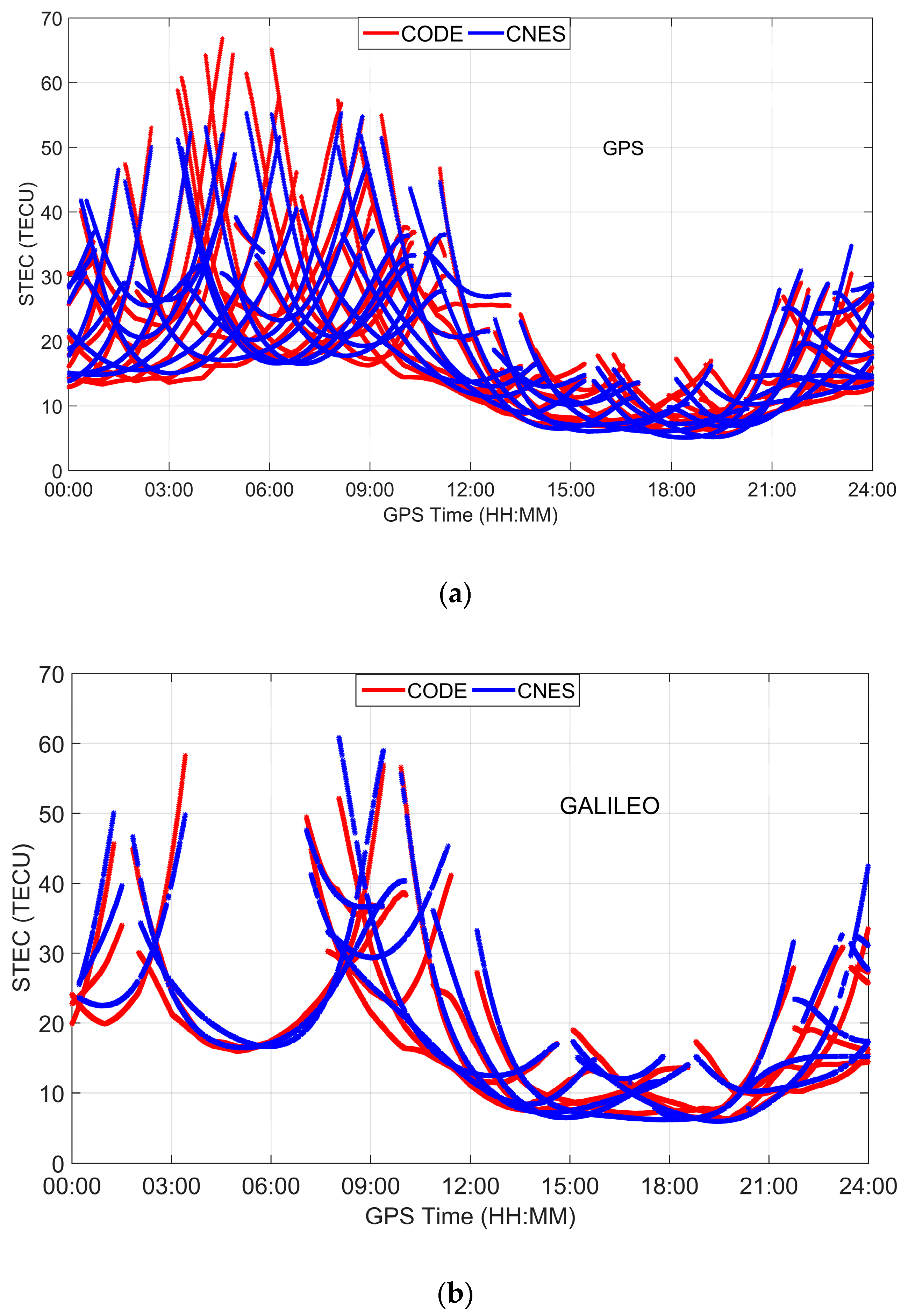
where is the ionospheric delay of the pseudo-observable, is the ionospheric mapping function as expressed in Equation (7), is the zenith angle from the satellites to the receiver, is the radius of the Earth (m) and is the height of the ionosphere shell (m), where the value of is 450 km for the products of CNES and CODE agency. Since the post-processing GIM products form CODE agency, that are computed by the stations distributed globally, has the highest accuracy (about 2~4 TECU) compared with those of other agencies [17], we use the post-processing GIM product as a reference to assess the RT ionosphere products. Figure 1 shows the slant TEC of GPS/GALILEO satellites for stations GMSD on day of year (DOY) 045, 2018. The slant TEC variation of RT ionosphere products and post-processing GIM products are quite consistent for a whole day, but there are obvious offsets with different products at some times, and the maximum offsets can be up to about 10 TECU, which is equivalent to a range error of about 1.6 m of the frequency of GPS. If the imprecise and unreliable variances of ionospheric constraint are used, these offsets have a negative impact on the accuracy of positioning.
2.3. Weight Factors Searching Algorithm with Moving-Window Average Filter
In order to achieve fast convergence and high-accuracy positioning solutions after convergence, a weighting approach is presented which combines a weight factors searching algorithm and a moving-window average filter. The weight factors searching algorithm is similar to the method of Helmert variance component estimation; it is based on the principle that the post-fit weighted sum residuals of squares is the minimum. A moving-window average filter is applied to improve the precision and reliability of this searching algorithm.
When RT ionospheric products are introduced, the variances matrix of measurement errors and measurement error vector in the Extended Kalman Filter (EKF) can be written as follows [18]:
where the subscript “” and “” denote the raw observation (pseudorange and phase measurements) and ionospheric constraints, respectively. The variance matrix of observation errors depends on the elevation of satellite and can be expressed as follows [19]:
In the Equation (10), the value of the standard deviation for GPS/GALILEO are set as 1 m and 0.01 m for the pseudorange and phase observations, respectively. Different from the variance matrix of observation, the variance of ionospheric constraints would be expressed as a product of a weight factor and an initial variance matrix , as follows:
The initial ionospheric constraints are set as the same as of pseudorange observations (this value of is suggested in PPP-WIZARD ducumentation). The computation procedure of the weight factors searching algorithm comprises the following steps:
- (1)
- Assign an initial weight factor () to the variance of ionospheric constraints .
- (2)
- Initialize the variance matrix of measurement errors by using Equation (10) and (11).
- (3)
- Compute post-fit measurement error vector after performing the EKF.
- (4)
- Compute the post-fit weighted sum residuals of squares .
- (5)
- Update the weight factor , where is a search space, which will be determined through the case studies later in the paper.
Repeat steps (2)–(5) to find the optimal weight factor that satisfies the following equation:
After step (6) is fulfilled, the final variance matrix of measurement errors can be determined by using the optimal weight factor .
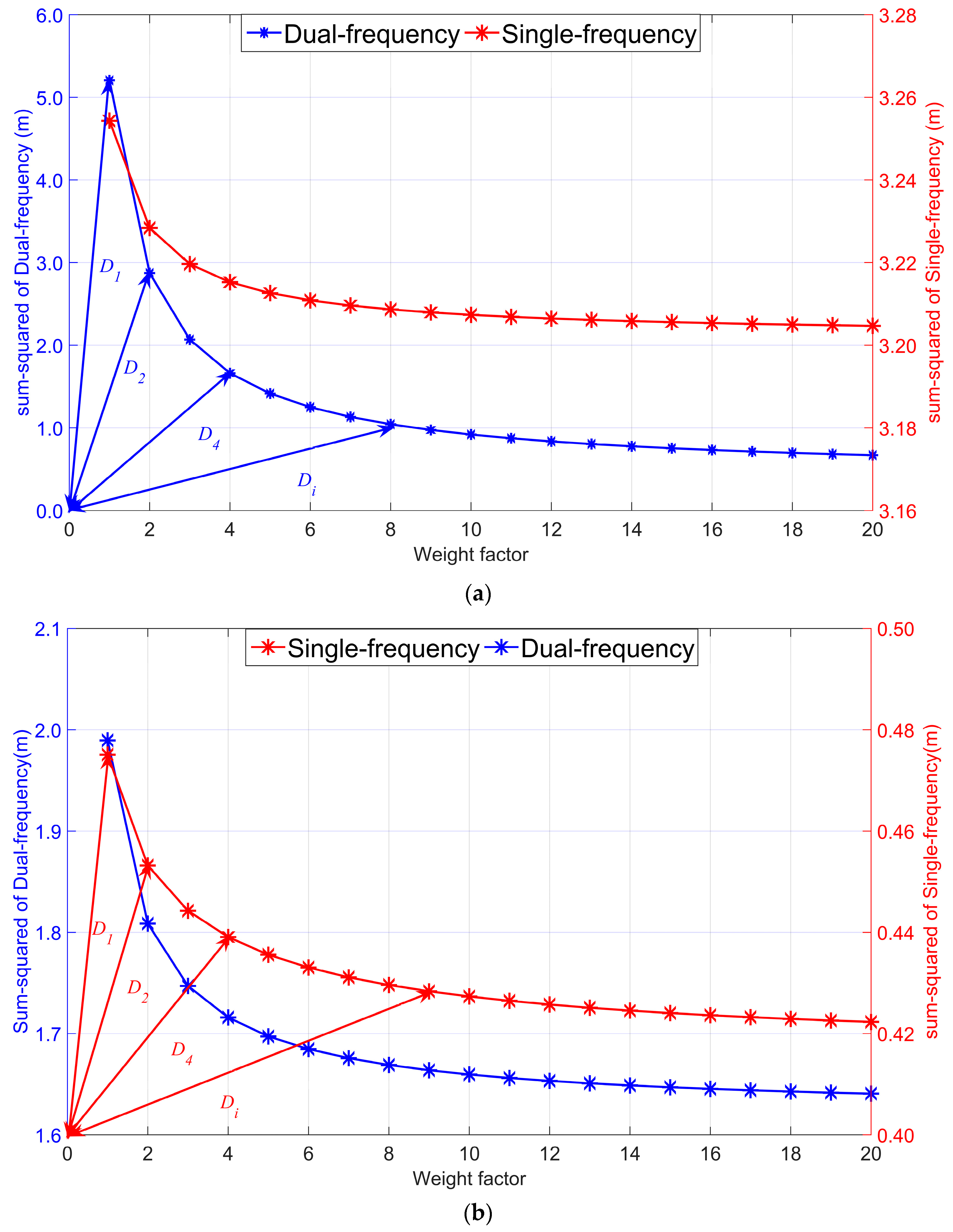
In order to determine a suitable search space of the weight factors searching algorithm, different positioning modes are conducted with ionospheric constraints. Figure 2 displays the relationships between the weight factors and the post-fit weighted sum-squared residuals. It is clearly seen that varying trend of post-fit sum-squared residuals are quite consistent in different positioning modes. Due to the imprecise used in RT PPP, the post-fit weighted sum residuals of squares is large when the variance matrix of ionospheric constraints is small. As the weight factor increases, the ionospheric constraints are weakened, and the post-fit weighted sum residuals of squares decreases gradually and then tends to be convergent. It was found that different positioning modes have the same characteristics, the post-fit weighted sum residuals of squares was close to stable when the distance between the point and the origin of the coordinate is the shortest. Therefore, to improve the efficiency of the searching algorithm, the Equation (12) can be replaced:
where subscript “” denotes search of searching algorithm, is the distance from the point to origin of the coordinate. If the distance is greater than distance , the search will be stopping and the of searching will be taken as the optimal weight factor.
Since the epoch-by-epoch determines the optimal weight factor, is not always available due to the limited number of the visible satellites and low redundancy of single-epoch data. To further enhance the reliability of the solutions, a moving-window average filter is applied to determine the smoothed optimal weight factor as follows:
where is the size of the smoothing window in average filter, is a smoothed optimal weight factor over multiple epochs within a time window from epoch to epoch . A long window size would tend to blend these changes into the previous open sky conditions, while a short one would change quickly to the conditions but would be prone to larger errors [20]. Since the observation data of MGEX station is obtained under good operating conditions, a suitable window size is set as 10. The effectiveness of this window size will be verified through experiments later in the paper.
3. Results and Analysis
3.1. Data Description and Process Schemes
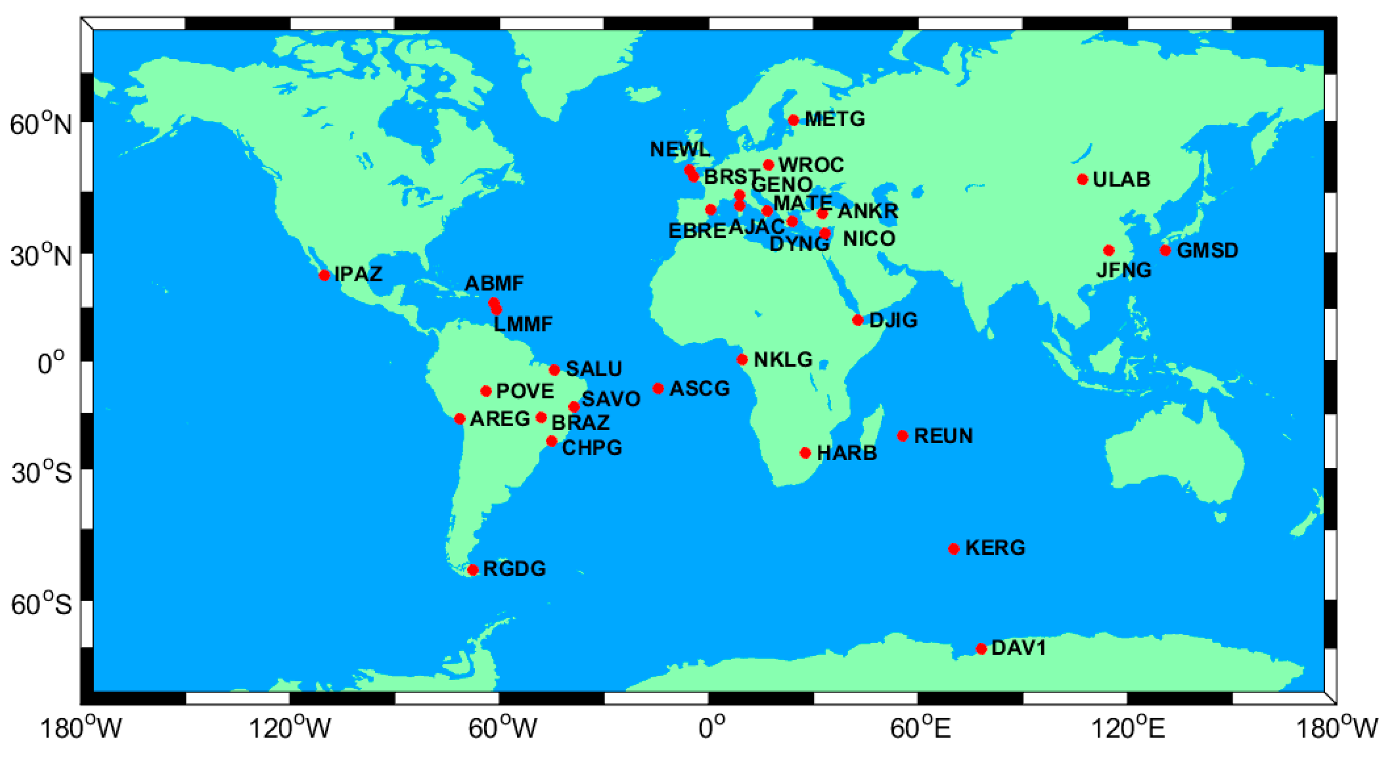
In order to test the proposed weighting approach for GPS/GALILEO RT PPP with ionospheric constraints, both static and kinematic experiments are conducted at single- and dual-frequencies. Three data processing methods, as listed in Table 1, were established to evaluate the impact on convergence time and positioning with different variances of ionospheric constraint. The first is using the GPS/GALILEO raw observations without ionospheric constraints, and the estimated parameter vector can be expressed as Equation (4). The second method is to determine the weight between observations and ionospheric constraints using priori variances by Equation (10). The third method is to determine the weight using the proposed approach. The estimated parameter vector of the second and the third method can be expressed as Equation (5). As shown in Figure 3, the observation data of 31 MGEX stations for 30-days (23 January 2018 to 23 February 2018) are selected. All these stations can track GPS/GALILEO satellites. The station coordinates were estimated every 30 s. The strategy of RT GPS/GALILEO PPP is summarized in Table 2. The RT precise orbit/clock correction and code/phase biases products in CLK92 stream from the CNES caster are used. Moreover, the correction of receiver PCO (phase center offset) and PCV (Phase Center Variations) for GALILEO are assumed to be the same as that of GPS.
3.2. Data Processing and Analysis
In GPS/GALILEO RT PPP, the position filter is considered to have converged when the absolute values of the positioning errors in East and North directions reach 0.1 m and keep within 0.1 m for consecutive 20 epochs (ten minutes) in dual-frequency static and kinematic cases. Given that the RT PPP errors in the single-frequency case are larger than those of dual-frequency case, the definition of the convergence of the single-frequency cases is enlarged to 0.3 m in the East and North directions. The convergence time is the period from the first epoch to the converged epoch. We compare the station coordinates calculated from different methods with coordinates supplied by IGS weekly solutions and calculate the RMS in three directions of them.
3.2.1. The Static RT PPP with Different Data Processing Methods
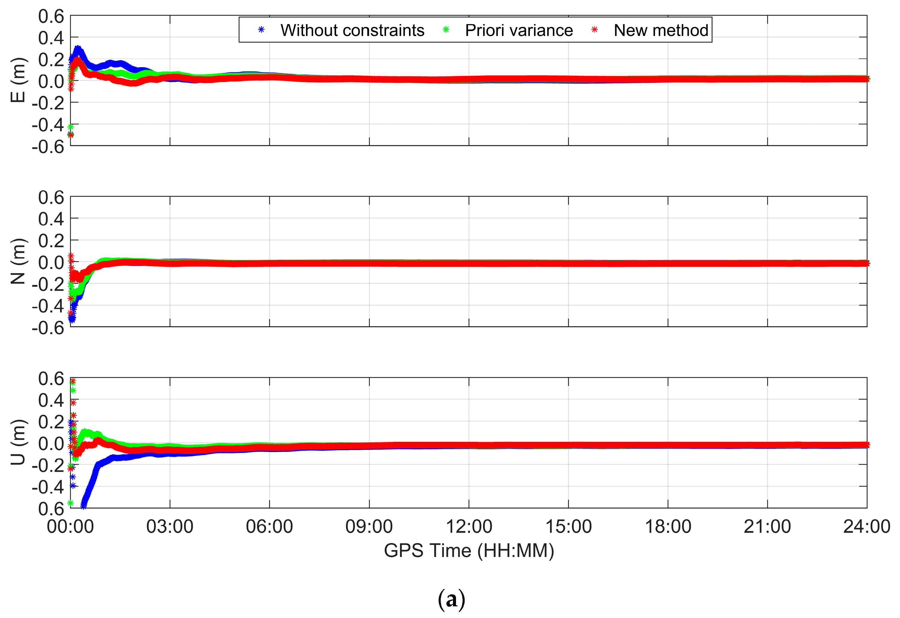
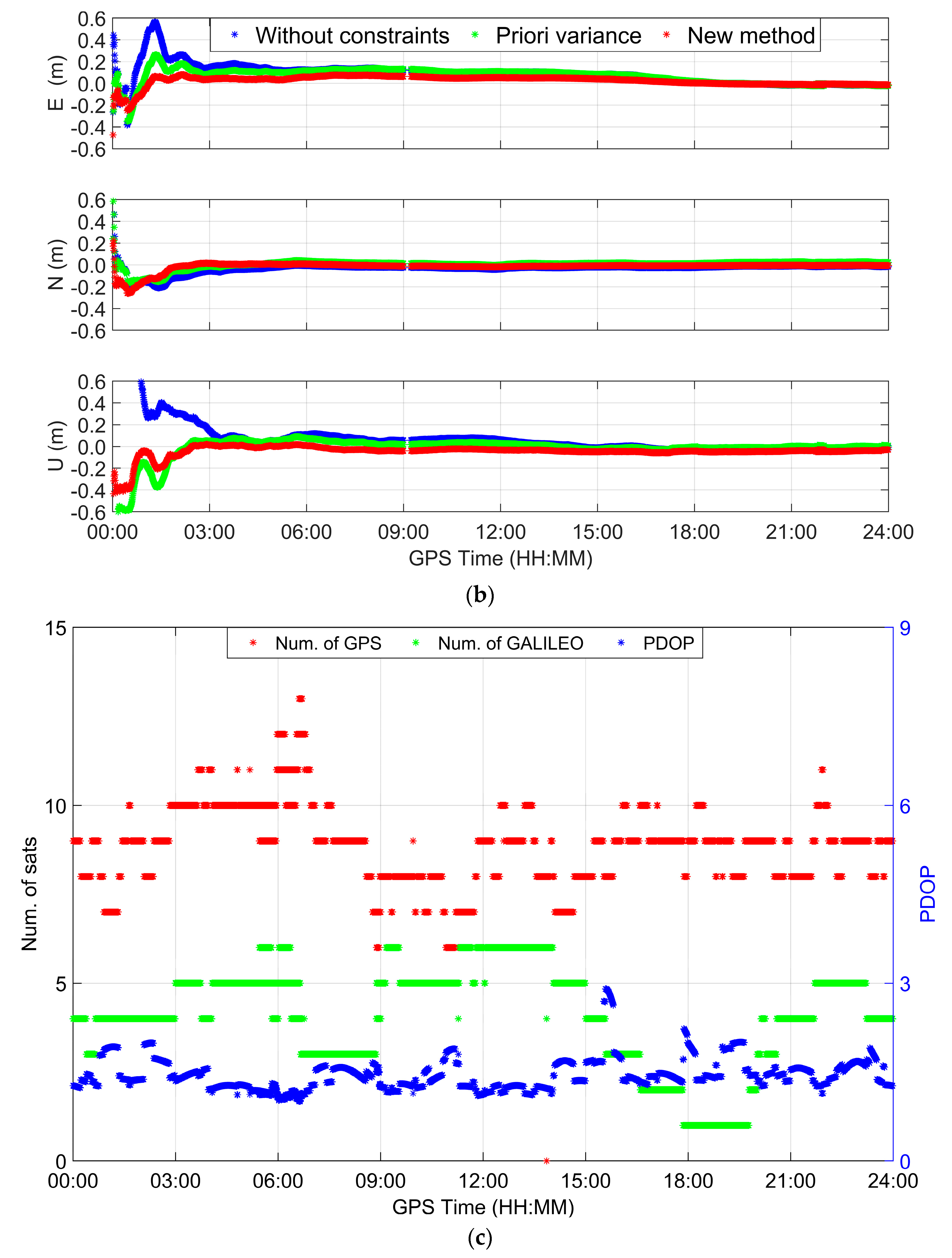
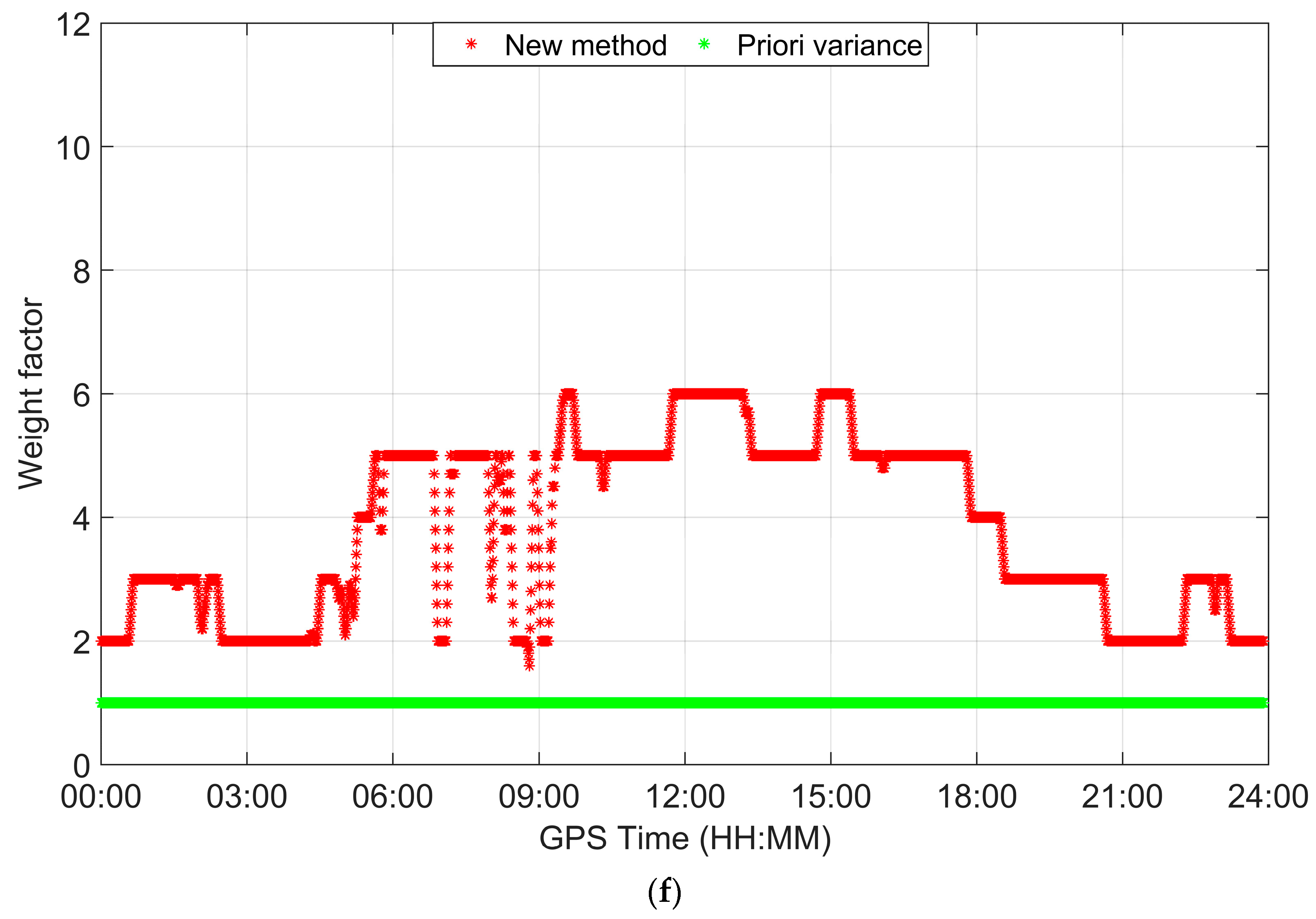
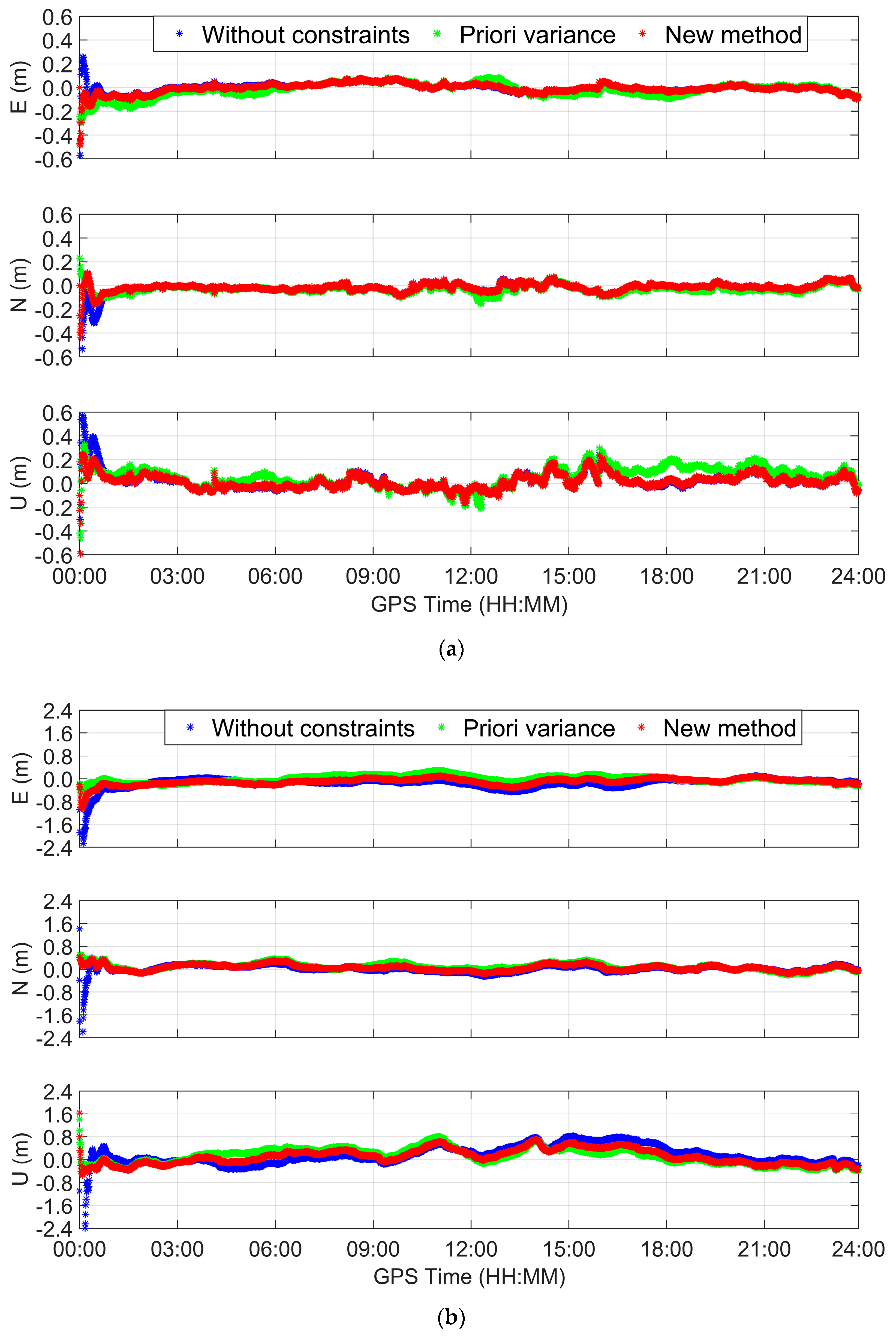
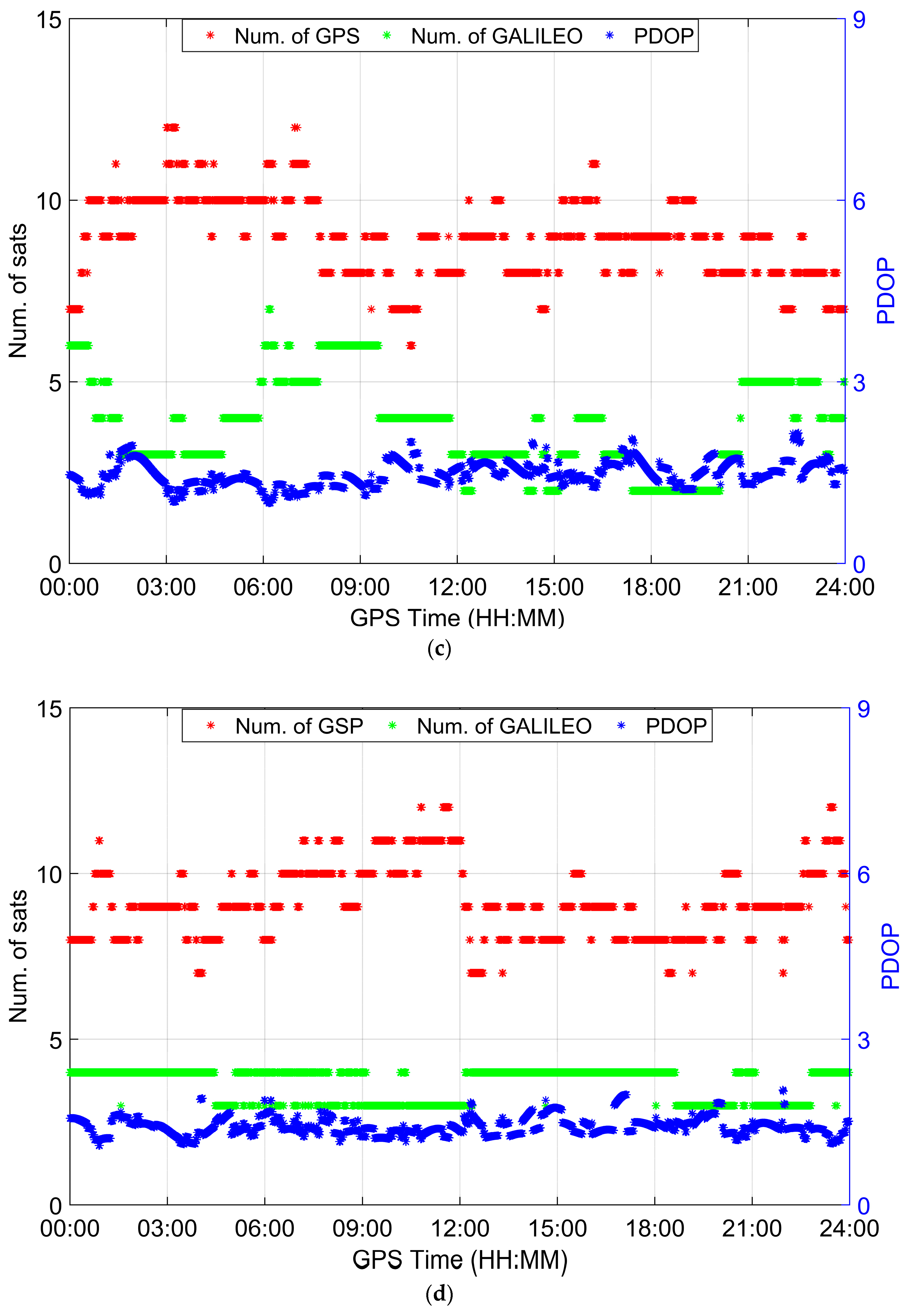
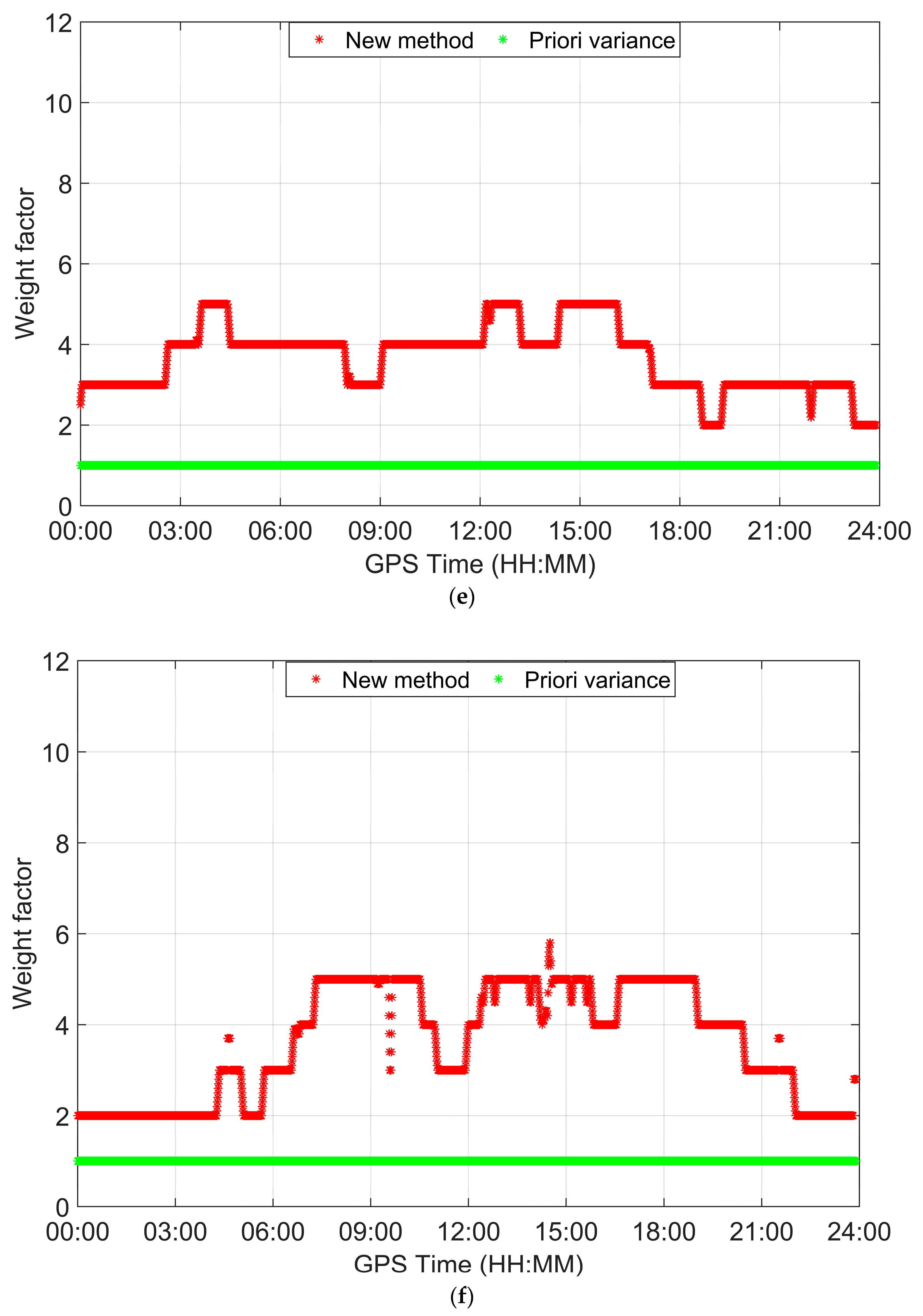
Figure 4a shows the positioning errors of static RT PPP with dual-frequency for stations ANRK on DOY 045, 2018. We can see that the result of three data processing methods is very similar when the filter converges to stable values. But there is great difference in convergence time with different processing methods. As seen from the blue curves, the convergence time of GPS/GALILEO RT PPP is about 116 min. After the ionospheric products are introduced for positioning with priori variance, it is clear that the convergence time can be reduced distinctly, especially in the UP direction. Compared with the priori variance method, the weights calculated by using new method are more reliable, and thus, convergence time can be further reduced; it only takes 26 min to achieve vertical accuracy of better than 0.1 m. The number of visible GPS/GALILEO satellites is shown in Figure 4b, together with the PDOP (position dilution of precision). The average number of visible GPS and GALILEO satellites are 9.3 and 5.4, respectively, leading to an average PDOP of 1.7. Figure 4c shows the weight factors of ionospheric constraints for different processing methods. The weight factors solutions vary in a range of 2.0 to 8.0 by using the new method. Since the priori variance for the ionospheric constraints does not correspond to reality, the weight factors of the new method are larger than that of a priori variance when the filter is not convergent; this is the reason why the convergence performance can be improved by using the new method.
To test the effectiveness of the new method in static single-frequency RT PPP, an experiment was conducted for station METG on DOY 051, 2018. Figure 4d shows the time series of single-frequency RT PPP positioning errors. The convergence performance of the without-constraints method is the worst of the three methods, especially in the East and Up direction, and its convergence time is up to 106 min. When ionospheric products are introduced as a pseudo-observable to constrain ionosphere delay in RT PPP, the convergence time can be reduced greatly. Using the new method, the convergence time is further reduced to 37 min and the positioning solutions are more precise than those of a priori variance. Figure 4f provides the weight factors for different processing methods. Due to the small weight factors calculated by the new method during the process of filter convergence, the contribution of ionospheric constraints is proper, and thus, convergence time can be reduced. The reason why positioning accuracy is high after filter convergence is that the weight factors calculated by the new method is larger than that of the priori variance method, and the contribution of low-accuracy (compared to carrier-phase measurements) RT ionospheric products is small. Table 3 summarizes the RMS of positioning error and convergence time for static single- and dual-frequency GPS/GALILEO RT PPP with three processing methods. The RMS computations are based on the position errors without considering the process of the filter convergence. From the Table 3, we can see that three methods have similar positioning accuracies after filter convergence in the dual-frequency case, but the positioning accuracy of the priori variance method becomes slightly worse than new methods in the single-frequency case. Compared to the other two methods, the proposed approach significantly improves convergence performance in static dual- and single-frequency cases. The convergence time improvement rate of the new method refers to the that of other two methods which are listed in the right column of “convergence time”, in which the largest improvement rate is 77%.
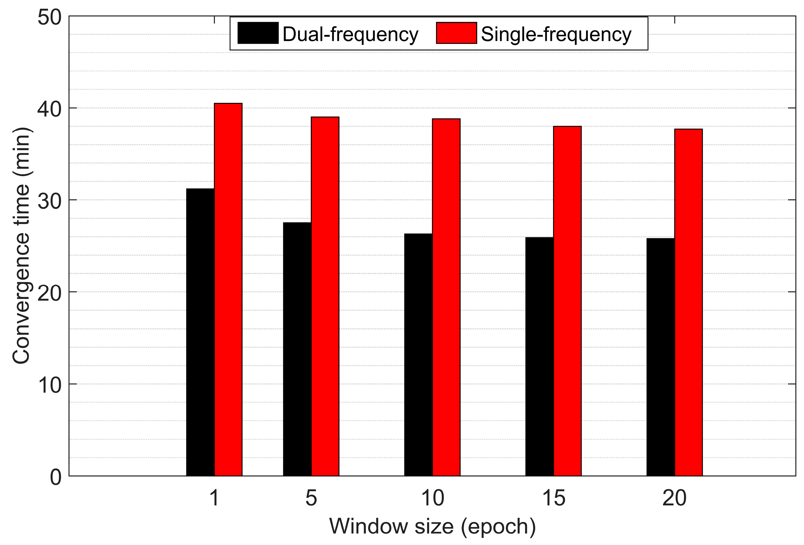
In order to ensure a reliable value of the window size in the proposed weighting approach, Figure 5 provides the convergence time of dual- and single-frequencies using different window sizes of 1, 5, 10, 15, and 20. As a result, the varying trend of convergence times is quite consistent in dual- and single-frequency cases, the improvement of the convergence time is less significant when the window size is increased from 10 to 20. This suggests that the window size of 10 is suitable, which will be applied for the rest of our data analysis.
3.2.2. The Kinematic RT PPP with Different Data Processing Methods
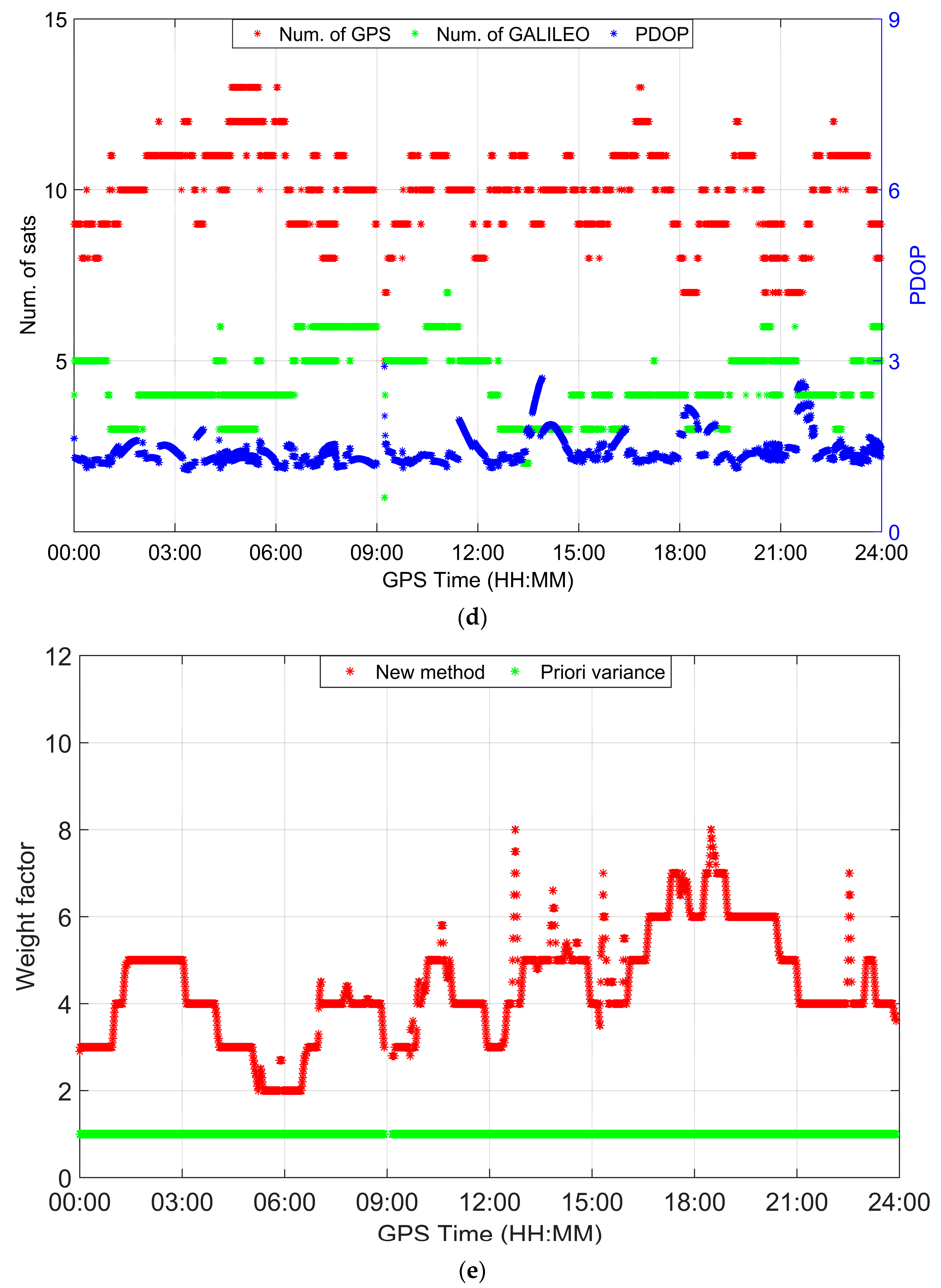
Different from static RT PPP positioning, the station coordinates will be estimated epoch-by-epoch in kinematic positioning. To assess the performance of the new weighting approach for single- and dual-frequency kinematic RT PPP, the datasets at MAT1 and WROC station on DOY 047, 2018 are conducted in the three processing methods.
The kinematic GPS/GALILEO RT PPP solutions with different methods are illustrated in Figure 6a,d for the dual- and single-frequency cases, respectively. The PDOP and number of satellites for MAT1 and KRGG station are provided in Figure 6b,e. Figure 6c,f shows the weight factors based on the new method and priori variance. We can find that the weight factors calculated by the new method are increased gradually when the positioning filter converges to a stable value, resulting in high-accuracy positioning solutions. Similar to the static RT PPP, we calculated the statistics of positioning accuracy and convergence times in different methods; these are given in Table 4. It is noted that both single- and dual-frequency convergence performance are improved after adding ionospheric constraints. Using our proposed approach, the RT PPP solution can converge within 15 min and 20 min for dual- and single-frequency cases, respectively, and the largest improvement rate can reach 73%. In terms of the RMS statistics of positioning errors, using the new method can achieve nearly the same positioning performance compared to the method without constraints. But using the priori variance method, obvious offsets exist in three directions after filter convergence, especially in the single-frequency case, which is caused by unreasonable weight in the ionospheric constraints.
3.2.3. Convergence Performance and Positioning Accuracy Assessment
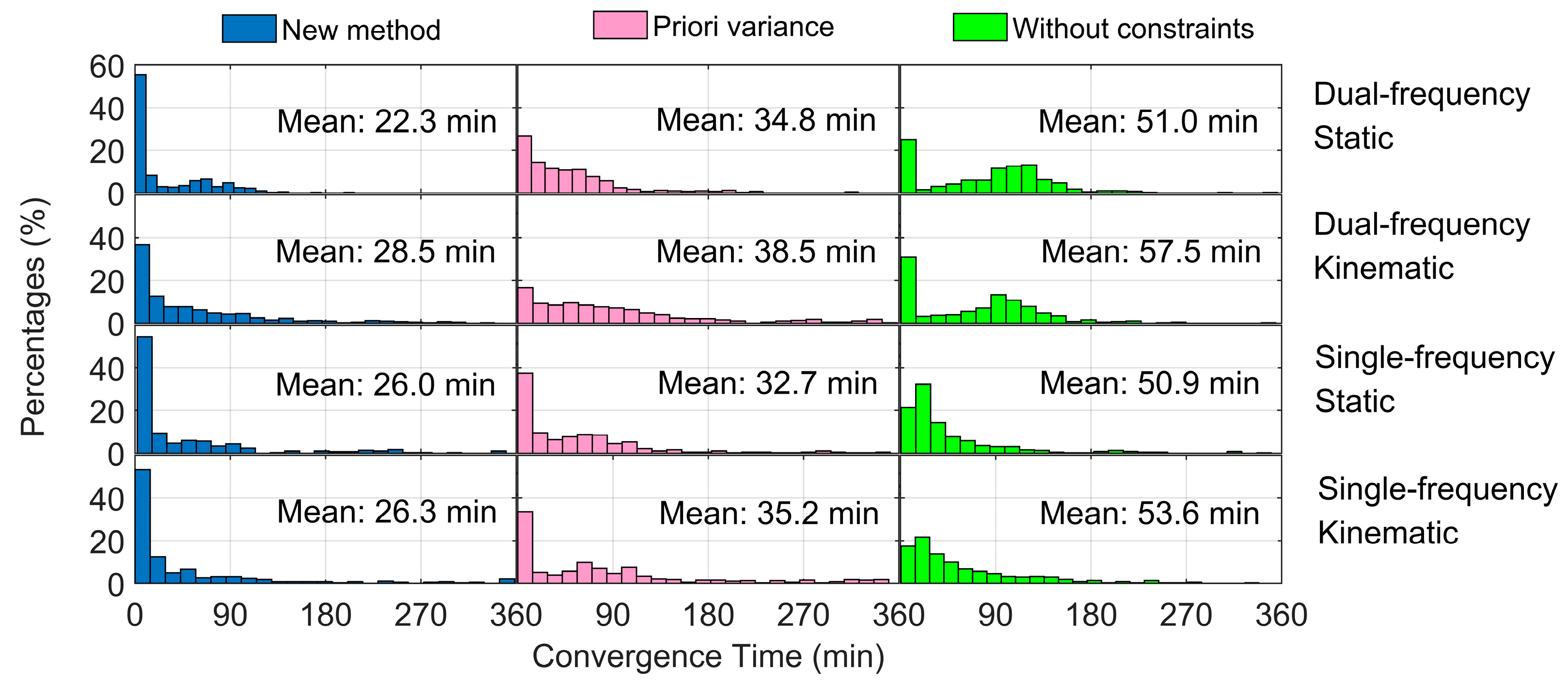
To further assess the convergence time and positioning accuracy in RT PPP using our proposed approach, the method of priori variance and without constraints, as listed in Table 1, are compared with a weight factors searching algorithm using datasets collected at 31 MGEX stations over 30 consecutive days from 23 January 2018 to 23 February 2018. A total of 11,160 sets of results are used to derive a statistical estimate on the convergence time as well as the positioning accuracy. The definition of the convergence time is the same as that described in Section 3.2. The distribution of the 11,160 sets of convergence times is plotted in minutes in Figure 7. It is observed that the performance of convergence can be improved in all positioning modes by using ionospheric constraints, but only to a slight degree. Using our proposed weighting approach, the convergence time of RT PPP is significantly decreased. The percentage of position solutions converging within 20 min is up to about 54%, 39%, 52%, and 50% in the dual-frequency static, dual-frequency kinematic, single-frequency static, and single-frequency kinematic positioning modes, respectively. The statistical results in terms of mean convergence time are also given in Figure 7. According to the mean values, the improvement of the new method on the convergence time is about 35.9%, 25.9%, 20.4%, and 25.2% over the method of priori variance in four positioning modes, respectively.
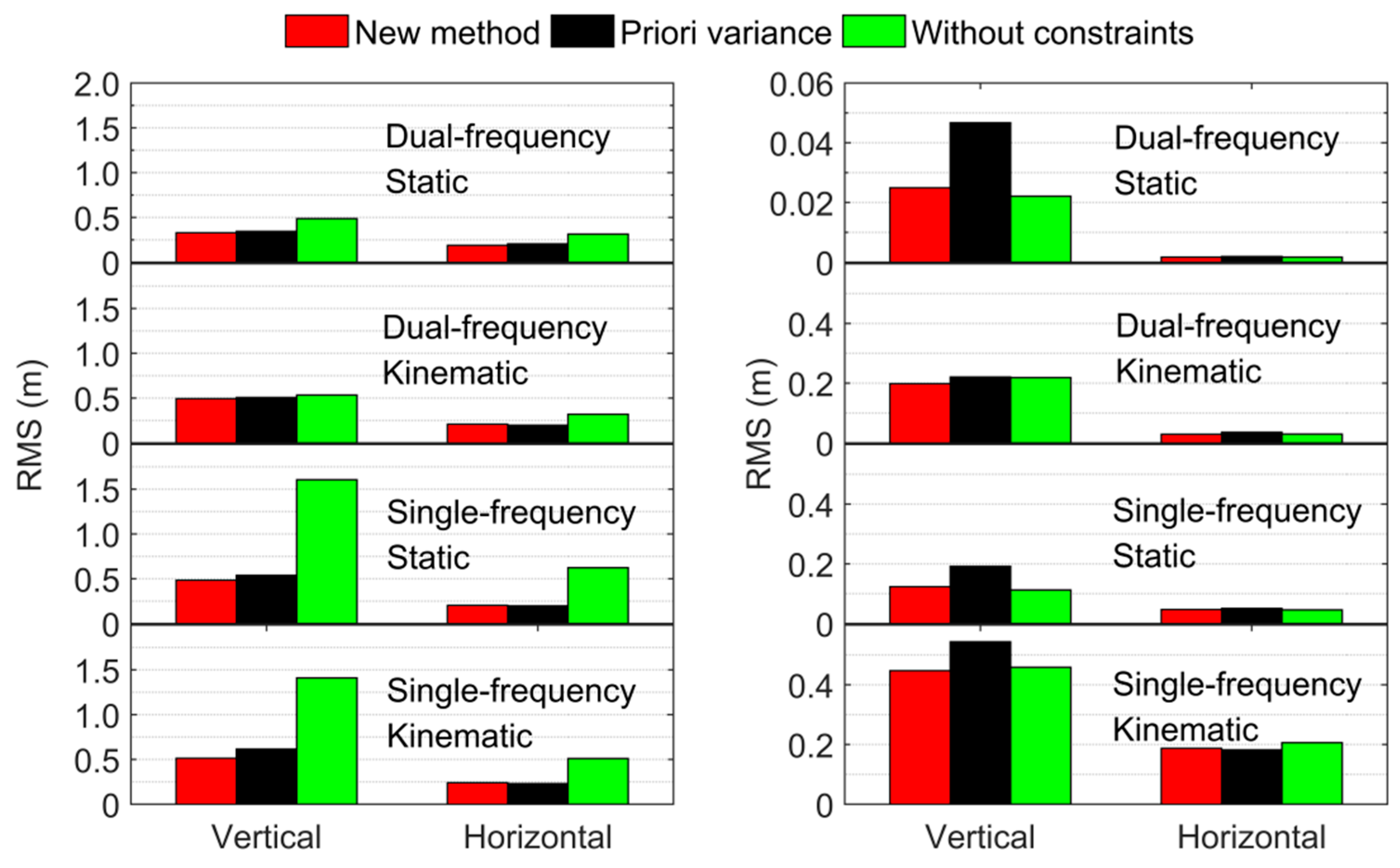
During the converging procedure of the RT PPP position filter, the size of position errors over time can also reflect the converging speed of the position filter [17]. Figure 8 illustrates the RMS statistical values of vertical and horizontal for all stations at the beginning of 30 min (left) and all day (right). Since the position solutions in the first two hours are still in the converging stage, they are not used for the accuracy statistics of all day. From the statistical results of 30 min, it is noted that positioning errors in four positioning modes sharply decrease after using RT ionospheric products at the beginning of the filter processing, especially in the single-frequency case. There is no denying that RT ionospheric products play an important role in accelerating filter convergence. But the method of priori variance exhibits slightly worse performance than the other two methods in the RMS statistical values of all day, as shown in Figure 8 (right), which indicates the negative impact of unreliable weighting on the convergence position accuracy. In terms of the RMS statistical values of all day, our proposed weighting approach can achieve the same precision as the method without constraints.
4. Conclusions
RT PPP can provide centimeter accuracy-level solutions based on real-time precise products, for orbits, clocks, and code/phase biases, provided by CNES. Nevertheless, a significant challenge for the RT PPP to achieve high-accuracy position solutions is its long convergence time, i.e., up to a few hours. Thanks to the standardization of RT message of VTEC models in CLK92/CLK93 stream from CNES, the convergence time of RT PPP can be reduced by using an uncombined functional model with RT ionospheric correction products. In order to significantly reduce the convergence time and achieve the high-accuracy positioning solutions after filter convergence, the proper weight of ionospheric constraints are important.
To solve this issue, a weight factors searching algorithm with a moving-window average filter is proposed. This approach is similar to the method of Helmert variance component estimation; it searches for the optimal weight of ionospheric constraints according to the principle that the sum of the quadratic forms of weighted residuals is the minimum, and makes good use of the weight information at previous epochs. Datasets collected at 31 MGEX stations on 30 consecutive days are exploited to evaluate the proposed approach. Both static and kinematic experiments have been carried out in dual- and single-frequency, and the statistical results indicate that the new method significantly improves the performance of RT PPP convergence. The maximum improvement reaches 35.9% in comparison to the method of priori variance. By using the new method, the final positioning accuracy is not affected by the accuracy of RT ionosphere products, and the same accuracy as that of without constraints can be achieved. Overall, our proposed weighting approach can not only accelerate the convergence at the beginning of filter processing, but can also achieve high-accuracy position solutions after filter convergence. Future work will include the application of the proposed weighting approach to multi-GNSS combinations with tropospheric constraints.
Author Contributions
T.L., J.W. and H.Y. came up with the idea of the constrain method, T.L. and X.C. analyzed the data, T.L. and Y.G. conceived and designed the experiments. T.L. wrote the paper.
Funding
The Fundamental Research Funds for the Central Universities with a grant number as 2015XKMS051.
Acknowledgments
The authors gratefully acknowledge Center National d’Etudes Spatiales (CNES) and IGS Multi-GNSS Experiment (MGEX) for providing GNSS data and precise products.
Conflicts of Interest
The authors declare no conflict of interest.
References
- Junior, O. Definition and Implementation of a New Service for Precise GNSS Positioning; UNESP: Sao Paulo, Brazil, 2018. [Google Scholar]
- Abdi, N.; Ardalan, A.A.; Karimi, R.; Rezvani, M.-H. Performance assessment of multi-GNSS real-time PPP over Iran. Adv. Space Res. 2017, 59, 2870–2879. [Google Scholar] [CrossRef]
- Laurichesse, D.; Privat, A. An open-source PPP client implementation for the CNES PPP-WIZARD demonstrator. In Proceedings of the ION GNSS+ 2015, Tampa, FL, USA, 14–18 September 2015; pp. 15–18. [Google Scholar]
- Geng, J.; Meng, X.; Dodson, A.H.; Ge, M.; Teferle, F.N. Rapid re-convergences to ambiguity-fixed solutions in precise point positioning. J. Geod. 2010, 84, 705–714. [Google Scholar] [CrossRef] [Green Version]
- Pan, L.; Xiaohong, Z.; Fei, G. Ambiguity resolved precise point positioning with GPS and BeiDou. J. Geod. 2016, 91, 25–40. [Google Scholar] [CrossRef]
- Laurichesse, D.; Langley, R. Handling the Biases for Improved TripleFrequency PPP Convergence. GPS World 2015, 26, 49–54. [Google Scholar]
- Li, X.; Ge, M.; Zhang, H.; Nischan, T.; Wickert, J. The GFZ real-time GNSS precise positioning service system and its adaption for COMPASS. Adv. Space Res. 2013, 51, 1008–1018. [Google Scholar] [CrossRef]
- Cai, C.; Gao, Y. Modeling and assessment of combined GPS/GLONASS precise point positioning. GPS Solut. 2012, 17, 223–236. [Google Scholar] [CrossRef]
- Lou, Y.; Zheng, F.; Gu, S.; Wang, C.; Guo, H.; Feng, Y. Multi-GNSS precise point positioning with raw single-frequency and dual-frequency measurement models. GPS Solut. 2015, 20, 849–862. [Google Scholar] [CrossRef]
- Li, P.; Zhang, X. Integrating GPS and GLONASS to accelerate convergence and initialization times of precise point positioning. GPS Solut. 2014, 18, 461–471. [Google Scholar] [CrossRef]
- Cai, C.; Gao, Y.; Pan, L.; Zhu, J. Precise point positioning with quad-constellations: GPS, BeiDou, GLONASS and Galileo. Adv. Space Res. 2015, 56, 133–143. [Google Scholar] [CrossRef]
- Li, W.; Teunissen, P.; Zhang, B.; Verhagen, S. Precise Point Positioning Using GPS and Compass Observations. In Proceedings of the China Satellite Navigation Conference (CSNC) 2013 Proceedings, Wuhan, China, 15–17 May 2013; pp. 367–378. [Google Scholar] [CrossRef]
- Zhang, H.; Hao, J.; Xie, J. The Weight Matrix Determination of Ionospheric Delay Constraintfor MultiGNSS Precise Point Positioning Using Raw Observations. Acta Geod. Cartogr. Sin. 2018, 47, 308–315. [Google Scholar] [CrossRef]
- Juan, J.M.; Hernández-Pajares, M.; Sanz, J.; Ramos-Bosch, P.; Aragon-Angel, A.; Orus, R. Enhanced Precise Point Positioning for GNSS Users. IEEE Trans. Geosci. Remote 2012, 50, 4213–4222. [Google Scholar] [CrossRef]
- RTCM Standard 10403.2. Differential GNSS (Global Navigation Satellite Systems) Services-Version 3; Radio Technical Commission for Maritime Services: Arlington, VA, USA, 2013. [Google Scholar]
- Schaer, S. IONEX: The ionosphere Map EXchange Format Version 1. In Proceedings of the Igs Analysis Center Workshop, Darmstadt, Germany, 9–11 February 1998. [Google Scholar]
- Cai, C.; Gong, Y.; Gao, Y.; Kuang, C. An Approach to Speed up Single-Frequency PPP Convergence with Quad-Constellation GNSS and GIM. Sensors 2017, 17, 1302. [Google Scholar] [CrossRef] [PubMed]
- Hernandez-Pajares, M.; Juan, J.M.; Sanz, J.; Ramos-Bosch, P.; Rovira-Garcia, A.; Salazar, D. The ESA/UPC GNSS-Lab tool (gLAB): An advanced multipurpose package for GNSS data processing. In Proceedings of the Satellite Navigation Technologies and European Workshop on GNSS Signals and Signal Processing, Noordwijk, The Netherlands, 8–10 December 2011; pp. 1–8. [Google Scholar]
- Gerdan, G.P. A comparison of four methods of weighting double difference pseudorange measurements. Surveyor 1995, 40, 60–66. [Google Scholar] [CrossRef]
- Cai, C.; Pan, L.; Gao, Y. A Precise Weighting Approach with Application to Combined L1/B1 GPS/BeiDou Positioning. J. Navig. 2014, 67, 911–925. [Google Scholar] [CrossRef] [Green Version]
- Wu, J.T.; Wu, S.C.; Hajj, G.A.; Bertiger, W.I.; Lichten, S.M. Effects of antenna orientation on GPS carrier phase. Astrodynamics 1991, 1993, 1647–1660. [Google Scholar]
- Petit, G.; Luzum, B. IERS Conventions. Bureau International des Poids et Mesures Sevres (France). 2010. Available online: https://www.iers.org/IERS/EN/Publications/TechnicalNotes/tn36.html (accessed on 1 July 2017).
- Niell, A.E. Global mapping functions for the atmosphere delay at radio wavelengths. J. Geophys. Res.-Solid Earth 1996, 101, 3227–3246. [Google Scholar] [CrossRef]
- Teunissen, P. A Comparision of TCAR, CIR and LAMBDA GNSS Ambiguity Resolution. In Proceeding of the 15th International Technical Meeting of the Satellite Division of the Institute of Navigation, Portland, OR, USA, 24–27 September 2001; pp. 2799–2808. [Google Scholar]
- Ge, Y.; Zhou, F.; Sun, B.; Wang, S.; Shi, B. The Impact of Satellite Time Group Delay and Inter-Frequency Differential Code Bias Corrections on Multi-GNSS Combined Positioning. Sensors 2017, 17, 602. [Google Scholar] [CrossRef] [PubMed]
Figure 1.
Slant TEC of GPS (a) and GALILEO (b) derived from different agencies at station GMSD.

Figure 2.
Relationships between the weight factors and the post-fit weighted sum-squared residuals for kinematic (a) and static (b).
Figure 2.
Relationships between the weight factors and the post-fit weighted sum-squared residuals for kinematic (a) and static (b).

Figure 3.
The distribution of MGEX stations in the experiment.

Figure 4.
Static positioning errors (a,b), number of satellites, PDOP (c,d), weight factors (e,f) of dual-frequency RT PPP by station ANRK (a,c,e) and single-frequency RT PPP by station METG (b,d,f).
Figure 4.
Static positioning errors (a,b), number of satellites, PDOP (c,d), weight factors (e,f) of dual-frequency RT PPP by station ANRK (a,c,e) and single-frequency RT PPP by station METG (b,d,f).


Figure 5.
Convergence time using the proposed weighting approach with different smoothing window sizes for dual-frequency and single-frequency METG station.
Figure 5.
Convergence time using the proposed weighting approach with different smoothing window sizes for dual-frequency and single-frequency METG station.

Figure 6.
The kinematic positioning errors (a,b), number of satellites, PDOP (c,d), weight factors (e,f) of dual-frequency by station MAT1 (a,c,e) and single-frequency by station KRGG (b,d,f).
Figure 6.
The kinematic positioning errors (a,b), number of satellites, PDOP (c,d), weight factors (e,f) of dual-frequency by station MAT1 (a,c,e) and single-frequency by station KRGG (b,d,f).


Figure 7.
Distribution of convergence time for dual-frequency static, dual-frequency kinematic, single-frequency static, and single-frequency kinematic using datasets at 31 MGEX stations over thirty days.
Figure 7.
Distribution of convergence time for dual-frequency static, dual-frequency kinematic, single-frequency static, and single-frequency kinematic using datasets at 31 MGEX stations over thirty days.

Figure 8.
RMS statistics of positioning errors for different RT PPP processing methods at the beginning of 30 min (left) and all day (right).
Figure 8.
RMS statistics of positioning errors for different RT PPP processing methods at the beginning of 30 min (left) and all day (right).


Table 1.
List of Data Processing Methods.
| Modes | Details |
|---|---|
| Without constraint | GPS/GALILEO observations without ionospheric constraints |
| Priori variance | GPS/GALILEO observations+ionospheric constraints with a priori variance |
| New method | GPS/GALILEO observations+ionospheric constraints with proposed method |
Table 2.
Strategies for RT GPS/GALILEO PPP.
| Item | Setting |
|---|---|
| Observations | Raw pseudo range and phase observations |
| Frequency | GPS: L1/L2; GALILEO: E1/E5 |
| Estimator | Extended Kalman filter |
| Elevation cutoff | 10° |
| Sampling offset | 30 s |
| Observations weight | Elevation dependent weighting; 0.01 m and 1 m for GPS/GALILEO phase and pseudo range observables in zenith direction; |
| Phase windup | Phase polarization effects applied [21] |
| Attitude law | Nominal attitude for GPS and GALILEO |
| Station displacement | Solid Earth tides, ocean tide loading and pole tides [22] |
| A priori Troposphere delay | Saastamoinen model and Niell mapping function [23] |
| Zenith wet tropospheric delay | Estimated as random walk () |
| Ionosphere | Estimated as random walk processes (); |
| Station coordinate | Estimated as constant/white noise () in static/kinematic modes |
| Receiver clock | Estimated as white noise for each GNSS system |
| Satellite antenna PCO and PCV | PCV and PCO values for GPS/GALILEO were corrected with igs14.atx; |
| Receiver antenna PCO and PCV | Corrected by igs14.atx; Applied the same values as GPS to GALILEO; |
| Phase ambiguities | Float solution [24,25] |
Table 3.
Static RT PPP for three processing methods.
| Frequency | Methods | Convergence Time (min) | E (m) | N (m) | U (m) |
|---|---|---|---|---|---|
| Dual-frequency | Without constraint | 116 (77%) | 0.0033 | 0.0038 | 0.0346 |
| A priori variance | 50 (48%) | 0.0030 | 0.0039 | 0.0349 | |
| New method | 26 | 0.0019 | 0.0038 | 0.0336 | |
| Single-frequency | Without constraint | 106 (65%) | 0.0102 | 0.0748 | 0.0832 |
| A priori variance | 52 (28%) | 0.0129 | 0.0848 | 0.0732 | |
| New method | 37 | 0.0092 | 0.0687 | 0.0514 |
Table 4.
Kinematic RT PPP for three processing methods.
| Frequency | Methods | Convergence Time (min) | E (m) | N (m) | U (m) |
|---|---|---|---|---|---|
| Dul-frequency | Without constraint | 56 (73%) | 0.0682 | 0.0821 | 0.1186 |
| A priori variance | 38 (32%) | 0.0852 | 0.0798 | 0.1634 | |
| New method | 15 | 0.0568 | 0.0825 | 0.1183 | |
| Single-frequency | Without constraint | 61 (67%) | 0.1152 | 0.1007 | 0.3257 |
| A priori variance | 31 (35%) | 0.1655 | 0.1534 | 0.3760 | |
| New method | 20 | 0.1062 | 0.1186 | 0.3009 |
© 2018 by the authors. Licensee MDPI, Basel, Switzerland. This article is an open access article distributed under the terms and conditions of the Creative Commons Attribution (CC BY) license (http://creativecommons.org/licenses/by/4.0/).
Share and Cite
MDPI and ACS Style
Liu, T.; Wang, J.; Yu, H.; Cao, X.; Ge, Y. A New Weighting Approach with Application to Ionospheric Delay Constraint for GPS/GALILEO Real-Time Precise Point Positioning. Appl. Sci. 2018, 8, 2537. https://doi.org/10.3390/app8122537
AMA Style
Liu T, Wang J, Yu H, Cao X, Ge Y. A New Weighting Approach with Application to Ionospheric Delay Constraint for GPS/GALILEO Real-Time Precise Point Positioning. Applied Sciences. 2018; 8(12):2537. https://doi.org/10.3390/app8122537
Chicago/Turabian StyleLiu, Tianjun, Jian Wang, Hang Yu, Xinyun Cao, and Yulong Ge. 2018. "A New Weighting Approach with Application to Ionospheric Delay Constraint for GPS/GALILEO Real-Time Precise Point Positioning" Applied Sciences 8, no. 12: 2537. https://doi.org/10.3390/app8122537
Note that from the first issue of 2016, this journal uses article numbers instead of page numbers. See further details here.