Magnetic Levitation Control Based on Flux Density and Current Measurement

Featured Application

Active magnetic levitation.

Abstract

This paper presents an active magnetic levitation application that exploits the measurement of coil current and flux density to determine the displacement of the mover. To this end, the nonlinear behavior of the plant and the physical sensing principle are modeled with a finite element approach at different air gap lengths and coil currents. A linear dynamic model is then obtained at the operating point as well as a linear relation for the displacement estimates. The effectiveness of the modeling approach and the performance of the sensing and control techniques are validated experimentally on an active magnetic levitation system. The results demonstrate that the solution is able to estimate the displacement of the mover with a relative error below 3% with respect to the nominal air gap. Additionally, this approach can be exploited for academic purposes and may serve as a reference to implement simple but accurate active magnetic levitation control using low-cost, off-the-shelf sensors.

1. Introduction

Active magnetic levitation is found nowadays in industrial systems where contact-free operation is advantageous. Typical applications include the support of compressors, turbines and flywheels in vacuum, manufacturing, and oil-and-gas industrial fields [1,2,3,4]. High efficiency, low maintenance cost and control of the hovering dynamics are some of the key benefits of this technology [1,5].

In a nutshell, active magnetic levitation systems aim to control the position of the levitating object by varying the force imposed with an electromagnet. Their inherent nonlinear and unstable open loop nature motivate a substantial research effort mainly focused on the investigation of more effective actuator architectures [6,7] and the development of advanced control strategies to improve their dynamic performance, stability and robustness [8,9,10]. Additionally, since the performance of such systems is heavily influenced by the quality of the position feedback, the displacement sensing technique represents a crucial element. Typically, the displacement measurement is performed exploiting a variety of technologies such as optical, capacitive, magnetic, and electromagnetic sensing [1,11]. Optical sensors are easy to use and suitable for large air gaps [12], but prone to resolution loss due to diffraction effects [1]. Capacitive sensing features high resolution but is expensive and sensitive to dirt and dust [11,13]. Magnetic sensors have a good resolution but are sensitive to external magnetic fields [1]. Eddy-current and inductive sensors have good sensitivity, robustness, and immunity to dust [14,15,16]. Alternative solutions are the so-called self-sensing techniques, where the displacement sensor is not present, and the position of the levitating object is determined from the direct measurement of other variables, typically voltage and current in the electromagnet coil [1,17,18,19]. This reduces significantly cost, weight, and hardware complexity. A significant amount of research focuses on observer-based estimation relying on a mathematical model of the system [20,21,22]. Other techniques exploit the functional relationship between the magnetic circuit inductance and the position of the levitated object [23,24,25].

A further position sensing solution determines the displacement through the measurement of the flux density at the air gap along with the current flowing in the electromagnet coil. The addition of the flux density at the air gap with respect to the afore-mentioned self-sensing solutions improves the robustness and performance, while reducing the effects of plant-model mismatch and unmodeled dynamics [20,26]. However, in the authors’ knowledge, the literature related to this approach is limited. In [27], a Hall effect magnetic field sensor is installed between the electromagnet and the levitating object. A permanent magnet (PM) is also added to the levitating object. In this configuration, the sensed magnetic flux density is dominated by the behaviour of the PM and the displacement can be correlated with this measurement. However, as stated by the authors, the measurement of the magnetic flux density from the suspended object is corrupted by the magnetic behaviour of the coil, which is neglected in the sensing technique. This deficiency is addressed in [28] with a more precise sensing solution. The disturbance introduced by the solenoid field is evaluated numerically through a finite element (FE) model. A sensor fusion algorithm based on the unscented Kalman filter is adopted for the displacement estimation in real time.

This paper proposes a position control approach exploiting the measurements of the coil current and the magnetic flux density at the air gap to obtain the displacement of the mover. Unlike the aforementioned works, the mover is ferromagnetic and does not include any PM elements. In this case, the magnetic flux density strongly depends on both, the coil current and the mover position. This dependency is difficult to obtain analytically due to magnetic saturation on the mover, irregular or unknown flux paths, non-homogeneous air gap and leakage and stray flux effects. Therefore, FE simulations are carried out to identify the resulting nonlinear behaviour of the plant parameters (coil flux linkage and magnetic force) and the expected magnetic flux density measurement for different current and air gap length values. Subsequently, the model is linearized for a nominal operating point. A voltage control strategy is designed and implemented to validate the proposed solution on a simple magnetic levitation demonstrator. From an academic perspective, the proposed approach serves to illustrate fundamental principles of electrical and electronic engineering: electromagnetism and electrodynamics, control design, and practical implementation issues. Furthermore, users need to reinforce and understand the physics of the system due to the fact that the position sensor is not installed and indirect measurements are used instead.

The paper is structured as follows: Section 2 describes the general dynamic equations of the system and outlines the FE model. A linearized plant model and a method for displacement estimation are also introduced. Section 3 describes the levitator test rig, its main components and defines the design of the stabilizing controller. Section 4 presents the experimental results. Finally, Section 5 concludes the work.

2. Modeling

The magnetic levitation demonstrator consists of an electromagnet fixed to a frame and a levitated spherical body (mover), as illustrated in Figure 1. The electromagnet is an E-shaped core made of laminated soft iron with a coil wound on its central limb. The mover is devised with a thin soft iron yoke to reduce its mass.

Table 1. Geometric and layout features of the magnetic levitation demonstrator.

Subsystem	Property	Value	Unit
Electromagnet	Height	64	$\mathrm{mm}$
	Depth	17	$\mathrm{mm}$
	Limb width	16	$\mathrm{mm}$
	Slot width	16	$\mathrm{mm}$
	Total width	80	$\mathrm{mm}$
Coil	Wire gauge	0.5	$\mathrm{mm}$
	Number of turns	684	-
Mover	Outside diameter	92	$\mathrm{mm}$
	Yoke thickness	0.5	$\mathrm{mm}$
	Mass	67	$\mathrm{g}$

summarizes the main geometric and layout features of the described setup.

The system is governed by the following dynamic equations:

$$\begin{array}{cc}\hfill u& =\dot{\lambda }(i,q)+Ri,\hfill \end{array}$$

(1)

$$\begin{array}{cc}\hfill m\ddot{q}& =f_m(i,q)-f_d.\hfill \end{array}$$

(2)

Equation (1) describes the behavior of the coil circuit, where the input voltage u is contrasted by Ohm’s law through the coil resistance R and by Lenz’s law with the variation of the coil flux linkage $\lambda$ in time. The flux linkage $\lambda$ depends on the magnetomotive force applied to the magnetic circuit and the reluctance, which decreases with the air gap. Hence, $\lambda$ is a function of the vertical displacement q and the current i. Equation (2) defines the dynamic equilibrium of the mover body. The resultant force includes a magnetic component $f_m$ developed by the electromagnet and an external disturbance $f_d$ (usually the weight of the sphere). The force $f_m$ is a function of the vertical displacement coordinate q and the supply current i.

From the control point of view, the voltage u is the command input and the current i and flux density $B_s$ are the measured variables. This latter quantity is determined using an analog sensor installed on one of the side limbs of the electromagnet. Its role is to measure the flux density component $B_s$ which is orthogonal to the cross section of the sensing element (see Figure 1). The relation between $\lambda$, the current i and the vertical displacement q can be known either experimentally or from simulation. Thus, the measurement of $B_s$ and i allows to estimate q, provided that the magnetic hysteresis of the ferromagnetic parts is negligible.

The behavior of $\lambda$, $f_m$ and $B_s$ is necessary to implement any model-based control strategy on the described system. However, the analytical determination of these terms is not trivial due to magnetic saturation on the sphere yoke, irregular or unknown flux paths, non-homogeneous air gap, leakage and stray flux effects.

To simplify the analysis, the model is evaluated with the aid of a 3D finite element model in COMSOL Multiphysics. If losses in the iron domains are neglected, the electromagnetic problem formulation in terms of the magnetic vector potential $\mathbf{A}$ is given by

$$\begin{array}{c}\hfill \mathbf{B}=\mathbf{\nabla }\times \mathbf{A},\end{array}$$

(3)

$$\begin{array}{c}\hfill \mathbf{\nabla }\times \mathbf{H}={\mathbf{J}}_e,\end{array}$$

(4)

where $\mathbf{B}$ and $\mathbf{H}$ are the magnetic flux density and field vectors, respectively, and ${\mathbf{J}}_e$ is the external current density vector. Neglecting iron losses implies that the stated problem can be solved in a magnetostatic formulation, i.e., without the need for a computationally intensive time-stepping solution.

Air domains surrounding the actuator and inside the sphere are characterized by a unitary relative permeability with respect to vacuum. Soft iron domains, on the other hand, are represented with a nonlinear relation to account for saturation:

$$\begin{array}{c}\hfill \mathbf{H}=f_{\mathrm{Fe}}\left(\left|\mathbf{B}\right|\right)\frac{\mathbf{B}}{\left|\mathbf{B}\right|}\end{array}$$

(5)

The coil domain has the same magnetic properties as air. However, a specific feature of the software allows to define a homogenized multi-turn coil with external current density

$$\begin{array}{c}\hfill {\mathbf{J}}_e=\frac{N_{c}i}{A_c}{\mathbf{e}}_c,\end{array}$$

(6)

where $N_c$ is the number of turns of the coil, $A_c$ is its total cross section and ${\mathbf{e}}_c$ is a vector field representing the local direction of the coil wires. This latter term is determined by a coil geometry analysis study step embedded in COMSOL Multiphysics.

The symmetry of the model allows reducing the geometry size to one quarter, provided that the mover is perfectly centered with respect to the electromagnet. To decrease the computational overhead, this symmetry is exploited by imposing a Dirichlet’s boundary condition on all the surfaces of the model:

$$\mathbf{n}\times \mathbf{A}=\mathbf{0}$$

(7)

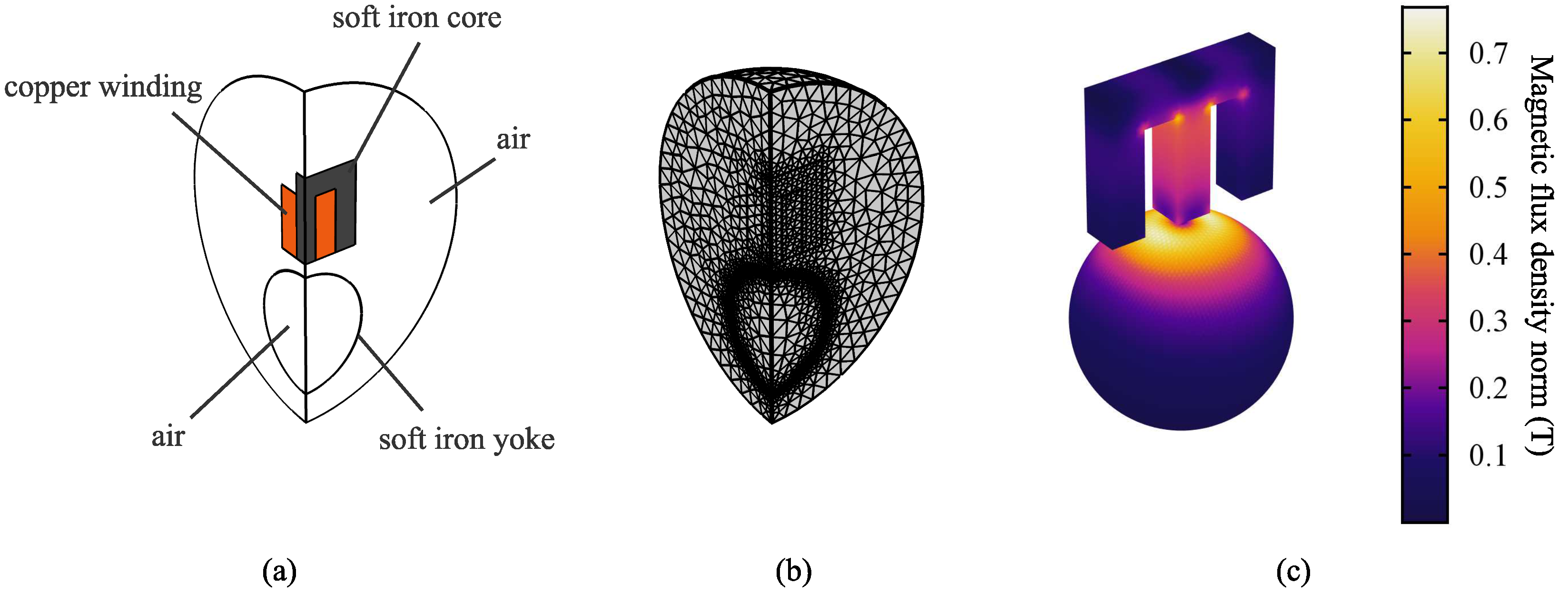
where n is the unit vector normal to the surface where the condition is applied. The resulting FE model is shown in Figure 2. It is simulated for a matrix of current and vertical displacement input values ranging from 0.1 to 1 $\mathrm{A}$ and 1 to 10 $\mathrm{mm}$, respectively. The coordinate q is assumed null when the mover is in contact with the central limb of the electromagnet and positive as the mover goes downwards.

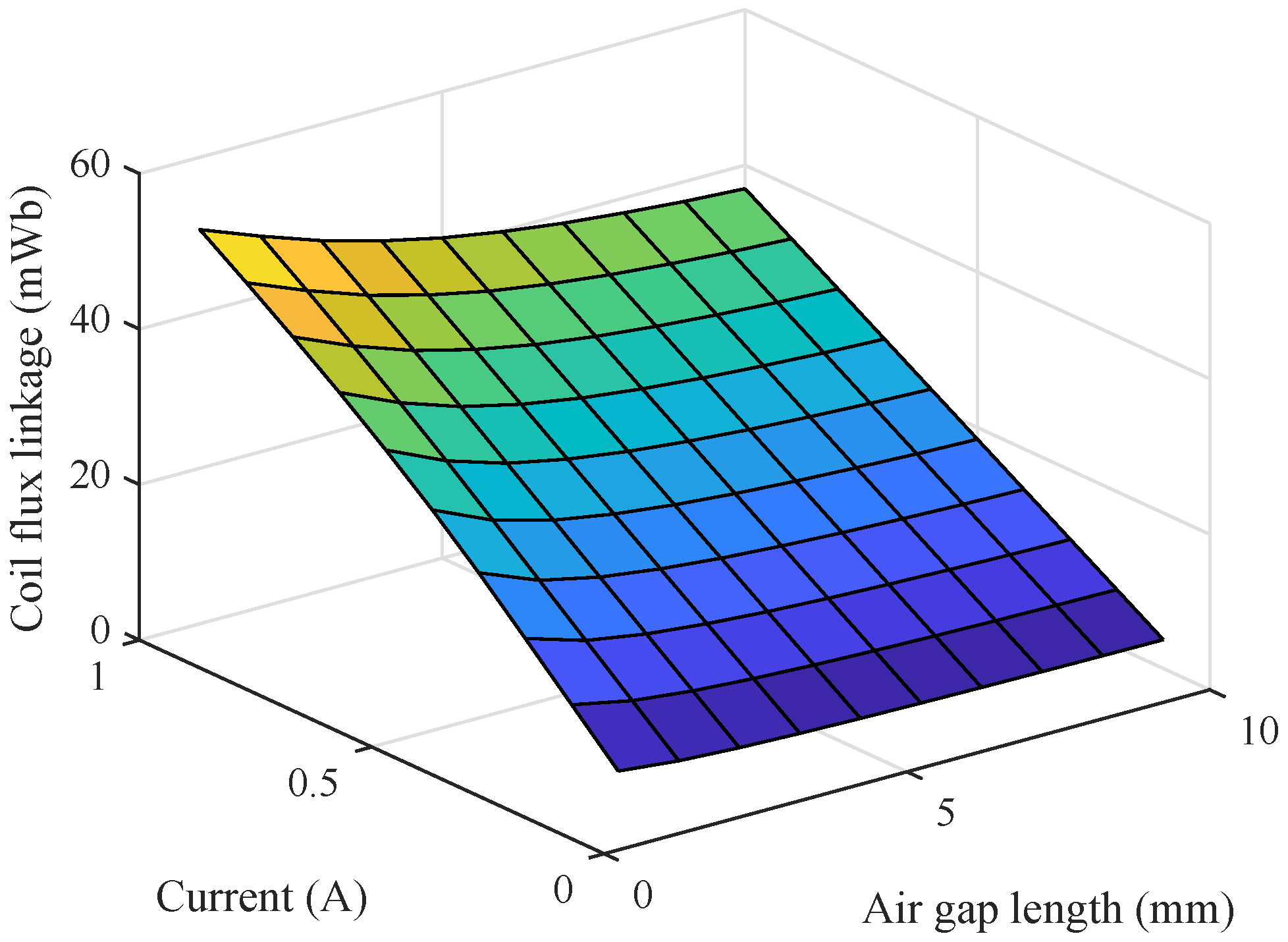
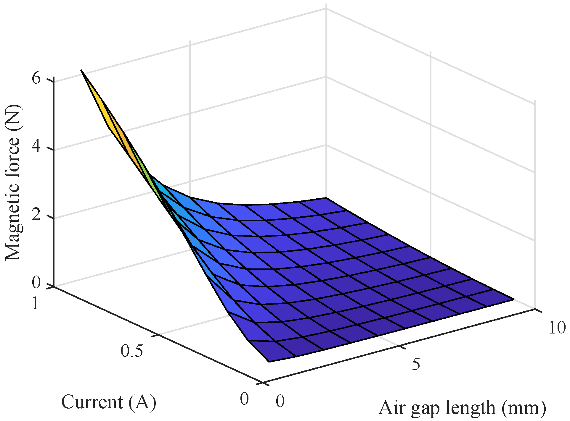
Figure 3, Figure 4 and Figure 5 illustrate the behavior of the analyzed terms for the working set of $(i,q)$ input pairs. It is observed that the variables exhibit nonlinear behavior with respect to the inputs. This is particularly emphasized for the magnetic force developed by the actuator. In addition, the coil flux linkage $\lambda$ and the measured magnetic flux density $B_s$ exhibit similar behaviors. Discrepancies are found when the mover is very close to the electromagnet because the flux on the side limb tends to change direction, while $B_s$ takes only the flux density component orthogonal to the cross section of the sensing element. Please note that the behavior of $B_s(i,q)$ is numerically defined in the examined range. Therefore, the measurements of $B_s$ and i can be used to determine indirectly the vertical position of the mover.

As an alternative to the numerical approach proposed here, the relation $B_s(i,q)$ (see Figure 5) could be characterized experimentally by adding a position sensor. However, a suitable position control is needed a priori to stabilize the plant and obtain reliable measurements. When applying a feedback control law, the flux density and the coil current values are prone to corruption due to feedback noise propagation.

2.1. Plant Model

Since the most important nonlinear dependencies of the plant have been numerically identified, the plant can be stabilized with any control technique. However, linearized models are usually preferred for control designers to exploit all the advantages of linear control theory. At any desired operating point, Equations (1) and (2) can be linearized and rewritten in terms of states $x={\left[qvi\right]}^T$ as a linear continuous-time state space representation

$$\begin{array}{cc}\hfill \left[\begin{array}{c}\dot{q}\\ \dot{v}\\ \dot{i}\end{array}\right]& =\left[\begin{array}{ccc}0& 1& 0\\ \frac{k_q}{m}& 0& \frac{k_i}{m}\\ 0& -\frac{k_v}{L_0}& -\frac{R}{L_0}\end{array}\right]\left[\begin{array}{c}q\\ v\\ i\end{array}\right]\hfill \\ & +\left[\begin{array}{cc}\begin{array}{c}0\\ 0\\ \frac{1}{L_0}\end{array}& \begin{array}{c}0\\ \frac{1}{m}\\ 0\end{array}\end{array}\right]\left[\begin{array}{c}u\\ f_d\end{array}\right],\hfill \end{array}$$

(8)

where

$$k_i=k_v={\left.\frac{\partial f_m}{\partial i}\right|}_{x_0},k_q={\left.\frac{\partial f_m}{\partial q}\right|}_{x_0},L_0={\left.\frac{\partial \lambda }{\partial i}\right|}_{x_0}.$$

The states $x={\left[qvi\right]}^T$ are hereinafter the deviation variables of the mover displacement, its speed and the coil current, respectively. The coefficients $k_q$ and $k_i$ are the well-known force-displacement and force-current factors [1,29], $L_0$ stands for the inductance and $k_v$ is the back-electromotive force coefficient. The coefficient $k_v$ is considered equal to $k_i$ due to energy conservation. All these parameters are numerically evaluated at the operating point $x_0$ from the FE simulations presented in the previous Section.

2.2. Displacement Estimation

As previously stated, a position sensor is not used and a combination of flux density and coil current measurements is proposed instead to calculate the mover displacement. To this end, the relation $B_s(i,q)$ (see Figure 5) can be linearized at the desired operating point $x_0={\left[q_0{v}_0{i}_0\right]}^T$ from the Taylor series first order approximation:

$$\begin{array}{cc}\hfill {\widehat{B}}_s& \approx B_0+{\left.\frac{\partial B_s}{\partial i}\right|}_{x_0}(\widehat{i}-i_0)+{\left.\frac{\partial B_s}{\partial q}\right|}_{x_0}(\widehat{q}-q_0)\hfill \\ & \approx B_0+k_{bi}(\widehat{i}-i_0)+k_{bq}(\widehat{q}-q_0).\hfill \end{array}$$

(9)

where ${\widehat{B}}_s$ and $\widehat{i}$ are the measurements of the flux density and the coil current, respectively. The term $\widehat{q}$ stands for the unmeasured position of the mover. When transforming (9) into the corresponding deviation variables at the operating point (i.e., $B={\widehat{B}}_s-B_0,i=\widehat{i}-i_0$ and $q=\widehat{q}-q_0$), the displacement can be directly calculated as

$$q=\frac{1}{k_{bq}}B-\frac{k_{bi}}{k_{bq}}i.$$

(10)

The absolute values of the coefficients $k_{bq}$ and $k_{bi}$ are hereinafter named sensing coefficients. It is worth mentioning that any other more accurate displacement estimation based on, for instance, lookup tables or polynomial approximations derived from Figure 5 can be applied. However, for the sake of clarity, the linear relation (10) of the displacement estimates with the current and flux density sensors is proposed here. It makes sense as long as the mover does not deviate significantly from the nominal position.

3. Experimental Setup

3.1. Test Rig

The experiments are conducted with the test rig shown in Figure 6. The current in the electromagnet coil is measured by an Amploc AMP25 Hall sensor (sensitivity $37\mathrm{mV}/\mathrm{A}$). An Allegro A1325 linear Hall-effect sensor (sensitivity $31.25\mathrm{mV}/\mathrm{mT}$) measures the flux density component $B_s$. The sensitivity of the current sensor is increased by winding the coil conductor through the sensor core ten turns. The power stage consists of a Pololu G2 High-Power Motor Driver 24v13 with a fixed PWM carrier set at 20 kHz and a 24-V DC voltage.

The control strategy is implemented in a Texas Instruments TMS320F28335 digital signal processor (DSP). The resolution of the analog-to-digital converter (ADC) module of the DSP and the PWM output is 12 bits in both cases. The sampling frequency of the ADC module is triggered by the PWM carrier at 20 $\mathrm{kHz}$. All the DSP peripherals are configured via MATLAB/Simulink using the embedded coder support package for Texas Instruments C2000 processors and Simulink Coder. These packages allow fast prototyping because the C code is generated from a high level graphical Simulink environment. The fundamental time step of the position control loop is set at 1 $\mathrm{ms}$, and data acquisition through Simulink matches this time step.

3.2. Control Design

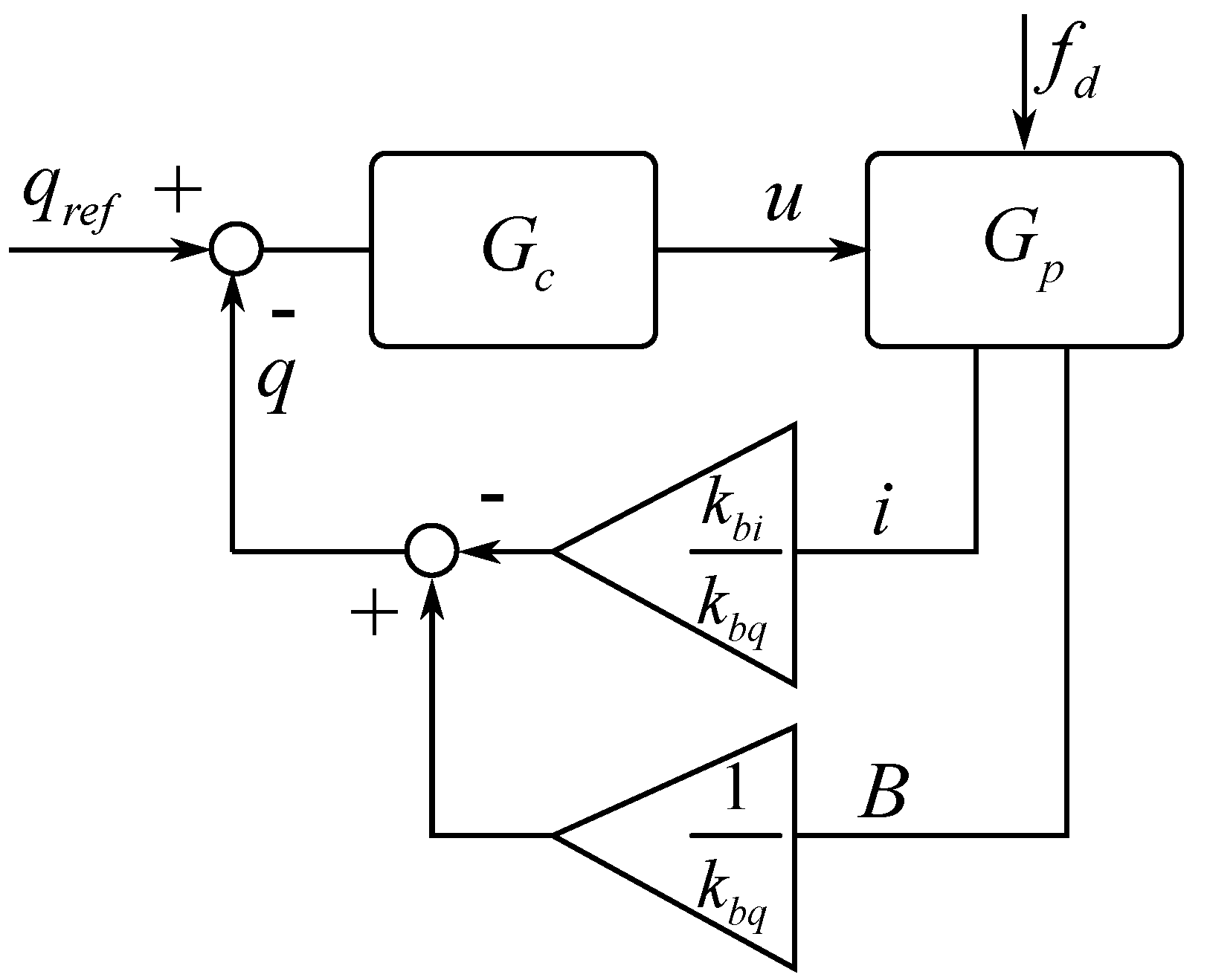
Any linear or nonlinear control technique could be applied and tested in the demonstrator since the plant is numerically identified by the FE simulations and the mover displacement is also known from current and flux density measurements. However, this work is intended only to assess the feasibility of applying an indirect sensing technique for an active magnetic levitation system. Hence, a linear, computationally inexpensive voltage control strategy is proposed as shown in Figure 7.

When using voltage control, the control requirements are hardly achievable if a conventional PID controller is used. According to [30], a convenient controller is a ${\mathrm{PD}}^2$ (i.e., two phase-lead compensator in series). However, since zero tracking error at steady state is desired, a small integral action is added and the resulting controller is the combination of a $\mathrm{PID}$ with a phase-lead compensator as

$$G_c=K_c\left(1+\frac{1}{{\tau }_{i}s}+\frac{{\tau }_d}{{\tau }_{f}s+1}\right)\frac{{\tau }_{1}s+1}{{\tau }_{2}s+1}.$$

(11)

The control requirements for the design are a phase margin between 30 and ${60}^{\circ }$, and the gain margin greater than $6\mathrm{dB}$ to guarantee stability even if the parameters of the plant model vary to a certain extent [31]. To this end, a linear model (8) is first obtained at $x_0$ and hence, the control parameters are selected accordingly.

4. Results and Discussion

Different tests are conducted to evaluate the plant-model mismatch, the correctness of the displacement estimation and the resolution of the sensing approach. The experimental results are obtained by selecting an air gap of $5\mathrm{mm}$ and the corresponding bias current $i_0=0.7\mathrm{A}$ to compensate the weight force. The measured coil resistance $R=3.4\mathsf{\Omega }$ is considered constant during the experiments and hence, a bias voltage $u_0=2.21\mathrm{V}$ is applied. As a result, there exists also a measured steady state flux density $B_0=12.88\mathrm{mT}$ which can be also corroborated from Figure 5.

For safety purposes, the coil voltage is bounded to $[0,2u_0]$ throughout the experiments to work only in the proximity of the nominal operating point $x_0$. This action avoids impulsive coil currents if the mover is manually removed. The resulting parameters of the plant model, the controller and the involved sensing coefficients at $x_0$ are presented in

Table 2. Plant Model, Controller and Sensing Parameters

Subsystem	Parameter	Value	Unit
Plant Model	$k_q$	216.30	$\mathrm{N}/\mathrm{m}$
	$k_i$	2.17	$\mathrm{N}/\mathrm{A}$
	$L_0$	41.21	$\mathrm{mH}$
	$k_v$	2.17	$\mathrm{Vs}/\mathrm{m}$
Controller	$K_c$	1000	$\mathrm{V}/\mathrm{m}$
	${\tau }_i$	0.20	$\mathrm{s}$
	${\tau }_d$	0.0125	$\mathrm{s}$
	${\tau }_f$	0.0021	$\mathrm{s}$
	${\tau }_1$	0.0125	$\mathrm{s}$
	${\tau }_2$	0.0021	$\mathrm{s}$
Sensing coefficients	$k_{bi}$	18.4	$\mathrm{mT}/\mathrm{A}$
	$k_{bq}$	0.8753	$\mathrm{mT}/\mathrm{mm}$

.

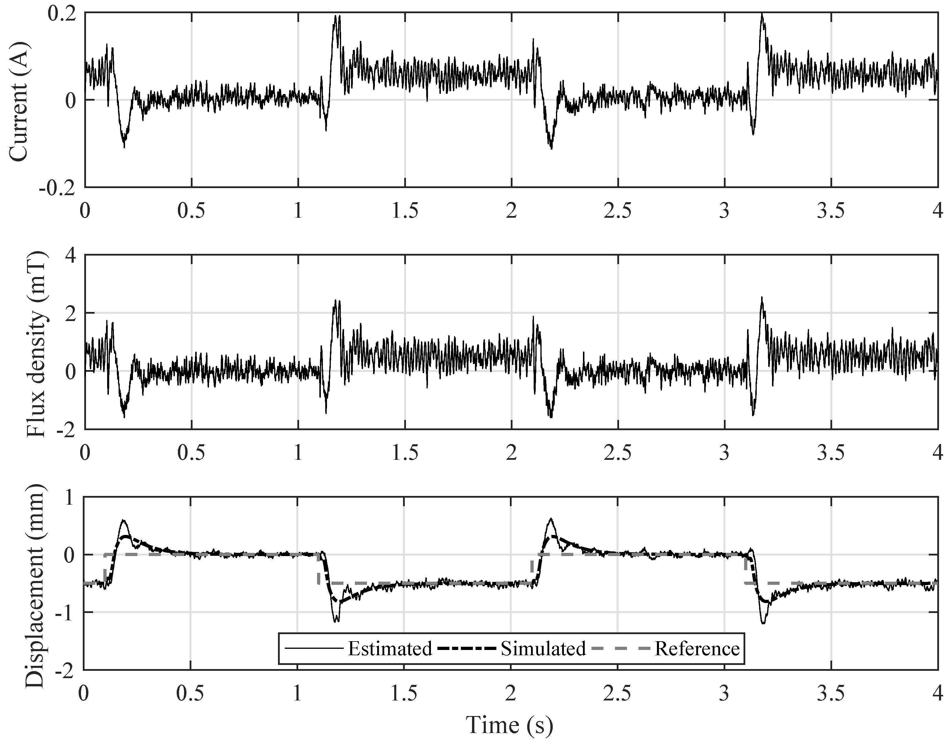
Transient responses of the system are presented in Figure 8 by varying the position reference $q_{ref}$. The obtained results prove the feasibility of applying the indirect sensing solution and the proposed control technique. The resulting linear model is sufficient to replicate the dynamics of the plant with a slight deterioration near the overshoots. This discrepancy is expected due to the nonlinear nature of the plant. Figure 8 also presents the unfiltered behavior of current and flux density measurements. However, a low-pass filter with a cut-off frequency at $300\mathrm{Hz}$ is applied before using them for the displacement estimation. This filter is accounted for the controller synthesis.

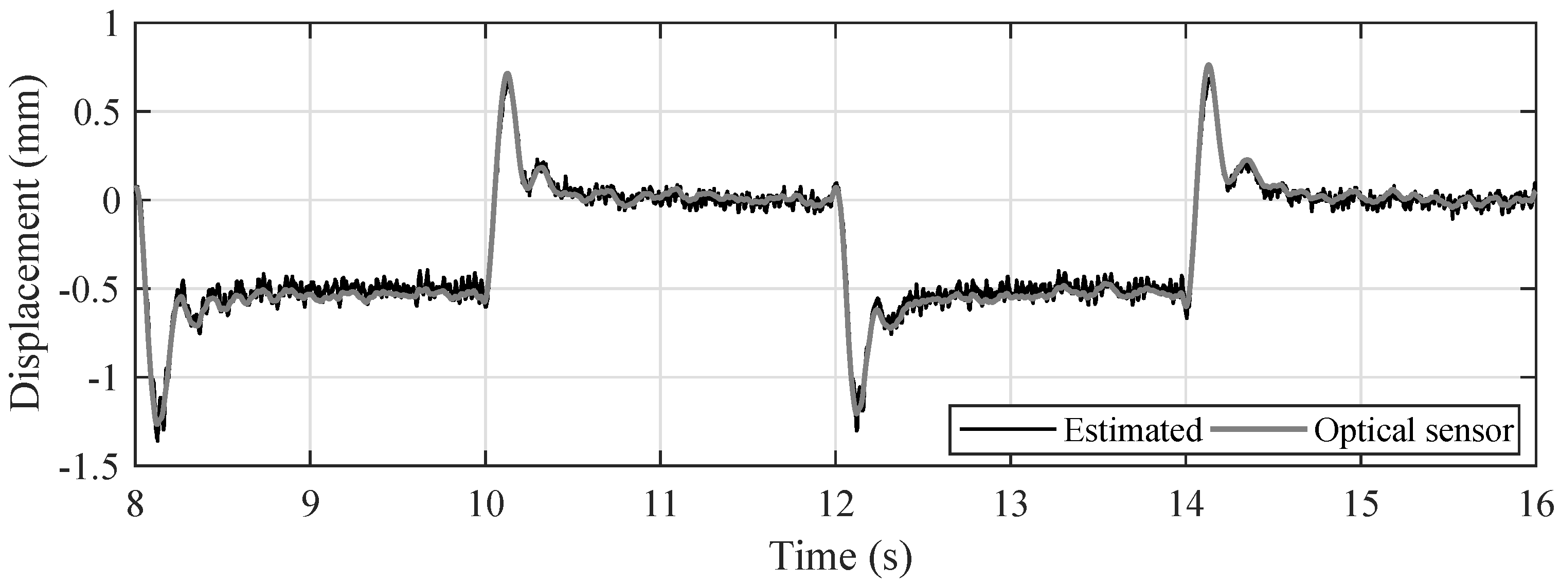
The correctness of the position estimates has been corroborated with a Micro-Epsilon optical displacement sensor LD1605-4 (sensitivity $5\mathrm{V}/\mathrm{mm}$, resolution $1\mathsf{\mu }\mathrm{m}$). Figure 9 shows both, the estimates and the sensor measurements when a reference step change is applied. Similarly, Figure 10 shows a quasi-static estimation behaviour around the nominal air gap. The position estimates match the sensor measurements with enough precision. The linear approximation (10) proved sufficient to estimate the mover displacement in the vicinity of the operating point. A slight but acceptable degradation of the position estimate is advisable when the sphere moves downwards and beyond the nominal operating point.

Figure 11 shows the open loop steady state behavior of the measurements from both sensors and the resulting displacement estimates. The data is obtained in a ten-second sampling window by fixing manually the mover at the nominal air gap while keeping the bias constant (i.e., the steady state condition at the operating point with the control voltage u set to $u_0$). The aim of this test is to inspect the resolution of the estimates from the measurements without the effect of the controller. The errors of the measurements are $\pm 6\mathrm{mA}$ and $\pm 69.8\mathsf{\mu }\mathrm{T}$ for the current and flux density sensors, respectively. These errors are amplified by the sensing gain blocks (see Figure 7) and propagated through the feedback loop. All in all, the displacement estimate error is bounded to $\pm 0.15\mathrm{mm}$ which is around $3\%$ of the nominal air gap. Please note that the uncertainty propagation is also affected by the resolution of the ADC module of the DSP. Nevertheless, since the system is inherently unstable, a stabilizing controller is mandatory for the levitation and therefore, the actual error under normal operation (i.e., controlled system) can differ according to the sensitivity of the control loop.

5. Conclusions

A simple, low-cost position control strategy on an active magnetic levitation demonstrator has been presented. The quasi-static nonlinear behavior of the magnetic force and flux linkage obtained from finite element simulations served to obtain a linear dynamic plant model once the operating point is selected. Furthermore, the numerical simulation of the measured flux density at different air gaps and coil currents allowed to identify the sensing coefficients involved in the displacement estimation. The nonlinear behavior of the plant is known a priori from numerical simulations, favoring significantly the synthesis of the control strategy. The proposed indirect sensing solution is able to estimate the displacement of the mover with a relative error below 3% with respect to the nominal air gap.

References

- Bleuler, H.; Cole, M.; Keogh, P.; Larsonneur, R.; Maslen, E.; Okada, Y.; Schweitzer, G.; Traxler, A.; Nordmann, R. Magnetic Bearings: Theory, Design, and Application to Rotating Machinery; Springer Science & Business Media: Berlin, Germmany, 2009. [Google Scholar]
- Yoon, S.Y.; Lin, Z.; Allaire, P.E. Control of Surge in Centrifugal Compressors by Active Magnetic Bearings: Theory and Implementation; Springer Science & Business Media: Berlin, Germmany, 2012. [Google Scholar]
- Hutterer, M.; Schrödl, M. Control of Active Magnetic Bearings in Turbomolecular Pumps for Rotors with Low Resonance Frequencies of the Blade Wheel. Lubricants 2017, 5, 26. [Google Scholar] [CrossRef]
- Li, X.; Anvari, B.; Palazzolo, A.; Wang, Z.; Toliyat, H. A Utility-Scale Flywheel Energy Storage System with a Shaftless, Hubless, High-Strength Steel Rotor. IEEE Trans. Ind. Electron. 2018, 65, 6667–6675. [Google Scholar] [CrossRef]
- Chiba, A.; Fukao, T.; Ichikawa, O.; Oshima, M.; Takemoto, M.; Dorrell, D.G. Magnetic Bearings and Bearingless Drives; Elsevier: Amsterdam, The Netherlands, 2005. [Google Scholar]
- Filatov, A.; Hawkins, L.; McMullen, P. Homopolar Permanent-Magnet-Biased Actuators and Their Application in Rotational Active Magnetic Bearing Systems. Actuators 2016, 5, 26. [Google Scholar] [CrossRef]
- Chen, S.L.; Weng, C.C. Robust control of a voltage-controlled three-pole active magnetic bearing system. IEEE/ASME Trans. Mechatron. 2010, 15, 381–388. [Google Scholar] [CrossRef]
- Maslen, E.; Montie, D. Sliding mode control of magnetic bearings: A hardware perspective. J. Eng. Gas Turbines Power 2001, 123, 878–885. [Google Scholar] [CrossRef]
- Bonfitto, A.; Castellanos Molina, L.; Tonoli, A.; Amati, N. Offset-Free Model Predictive Control for Active Magnetic Bearing Systems. Actuators 2018, 7, 46. [Google Scholar] [CrossRef]
- Javed, A.; Mizuno, T.; Takasaki, M.; Ishino, Y.; Hara, M.; Yamaguchi, D. Lateral Vibration Suppression by Varying Stiffness Control in a Vertically Active Magnetic Suspension System. Actuators 2018, 7, 21. [Google Scholar] [CrossRef]
- Boehm, J.; Gerber, R.; Kiley, N. Sensors for magnetic bearings. IEEE Trans. Magn. 1993, 29, 2962–2964. [Google Scholar] [CrossRef]
- Fama, R.C.; Lopes, R.V.; Milhan, A.; Galvão, R.; Lastra, B. Predictive control of a magnetic levitation system with explicit treatment of operational constraints. In Proceedings of the 18th International Congress of Mechanical Engineering, Ouro Preto, Brazil, 6–11 November 2005. [Google Scholar]
- Salazar, A.O.; Dunford, W.; Stephan, R.; Watanabe, E. A magnetic bearing system using capacitive sensors for position measurement. IEEE Trans. Magn. 1990, 26, 2541–2543. [Google Scholar] [CrossRef]
- Recheis, M.; Nicolics, J.; Wegleiter, H.; Schweighofer, B.; Fulmek, P. Evaluation of inductive displacement sensors for a basic active magnetic bearing test rig. In Proceedings of the 2011 34th International Spring Seminar on Electronics Technology (ISSE), Tratanska Lomnica, Slovakia, 11–15 May 2011; IEEE: Piscataway, NJ, USA, 2011; pp. 626–631. [Google Scholar]
- Klaučo, M.; Kalúz, M.; Kvasnica, M. Real-time implementation of an explicit MPC-based reference governor for control of a magnetic levitation system. Control Eng. Pract. 2017, 60, 99–105. [Google Scholar] [CrossRef]
- Noh, M.; Gruber, W.; Trumper, D.L. Low-cost eddy-current position sensing for bearingless motor suspension control. In Proceedings of the 2017 IEEE International Electric Machines and Drives Conference (IEMDC), Miami, FL, USA, 21–24 May 2017; IEEE: Piscataway, NJ, USA, 2017; pp. 1–6. [Google Scholar]
- Mizuno, T. Towards Practical Applicatitons of Self-Sensing Magnetic Bearings. In Proceedings of the Third International Symposium on Magnetic Bearings, Washington, DC, USA, 29–31 July 1992; Volume 169. [Google Scholar]
- Vischer, D.; Bleuler, H. Self-sensing active magnetic levitation. IEEE Trans. Magn. 1993, 29, 1276–1281. [Google Scholar] [CrossRef]
- Bonfitto, A.; Tonoli, A.; Silvagni, M. Sensorless active magnetic dampers for the control of rotors. Mechatronics 2017, 47, 195–207. [Google Scholar] [CrossRef]
- Maslen, E.H.; Montie, D.T.; Iwasaki, T. Robustness limitations in self-sensing magnetic bearings. J. Dyn. Syst. Meas. Control 2006, 128, 197–203. [Google Scholar] [CrossRef]
- Zingerli, C.M.; Kolar, J.W. Novel observer based force control for active magnetic bearings. In Proceedings of the 9th International Power & Energy Conference (IPEC 2010), Singapore, 26–29 October 2010; Volume 2729, p. 21892196. [Google Scholar]
- Bobtsov, A.A.; Pyrkin, A.A.; Ortega, R.S.; Vedyakov, A.A. A state observer for sensorless control of magnetic levitation systems. Automatica 2018, 97, 263–270. [Google Scholar] [CrossRef]
- Schammass, A.; Herzog, R.; Buhler, P.; Bleuler, H. New results for self-sensing active magnetic bearings using modulation approach. IEEE Trans. Control Syst. Technol. 2005, 13, 509–516. [Google Scholar] [CrossRef]
- Park, Y.H.; Han, D.C.; Park, I.H.; Ahn, H.J.; Jang, D.Y. A self-sensing technology of active magnetic bearings using a phase modulation algorithm based on a high frequency voltage injection method. J. Mech. Sci. Technol. 2008, 22, 1757–1764. [Google Scholar] [CrossRef]
- Glück, T.; Kemmetmüller, W.; Tump, C.; Kugi, A. A novel robust position estimator for self-sensing magnetic levitation systems based on least squares identification. Control Eng. Pract. 2011, 19, 146–157. [Google Scholar] [CrossRef]
- Siegwart, R.; Vischer, D.; Larsonneur, R.; Herzog, R.; Traxler, A.; Bleuler, H.; Schweitzer, G. Control concepts for active magnetic bearings. In Proceedings of the International Symposium on Magnetic Suspension Technology, Hampton, VA, USA, 19–23 August 1991. Part 2. [Google Scholar]
- Lundberg, K.H.; Lilienkamp, K.A.; Marsden, G. Low-cost magnetic levitation project kits. IEEE Control Syst. 2004, 24, 65–69. [Google Scholar]
- Chowdhury, A.; Sarjaš, A. Finite element modelling of a field-sensed magnetic suspended system for accurate proximity measurement based on a sensor fusion algorithm with unscented Kalman filter. Sensors 2016, 16, 1504. [Google Scholar] [CrossRef] [PubMed]
- Castellanos, L.; Bonfitto, A.; Tonoli, A.; Amati, N. Identification of Force-Displacement and Force-Current Factors in an Active Magnetic Bearing System. In Proceedings of the 18th Annual IEEE International Conference on Electro Information Technology, Rochester, MI, USA, 3–5 May 2018; pp. 3–5. [Google Scholar]
- Vischer, D. A new approach to sensor-less and voltage controlled AMBs based on network theory concepts. In Proceedings of the 2nd International Symposium Magnetic Bearing, Tokyo, Japan, 12–14 July 1990; pp. 301–306. [Google Scholar]
- Ogata, K. Modern Control Engineering; Prentice Hall: Upper Saddle River, NJ, USA, 2010; Volume 4. [Google Scholar]
Figure 1.
Model scheme of the magnetic levitation demonstrator.
Figure 2.
Finite-element 3D model of the levitation system: (a) geometry and domains; (b) mesh consisting of 109,210 elements; (c) magnetic flux density norm distribution for and , where the geometry is mirrored and the air domains are omitted for display purposes.
Figure 3.
Numerical behavior of the coil flux linkage as a function of current i and displacement q.
Figure 4.
Numerical behavior of the magnetic force as a function of current i and displacement q.
Figure 5.
Numerical behavior of the measured flux density as a function of current i and displacement q.
Figure 6.
Magnetic levitation demonstrator constituted by (1) frame, (2) base, (3) coil, (4) core, (5) magnetic flux density sensor, (6) mover, (7) power stage, (8) DSP development board, (9) current sensor, (10) power supply, (11) personal computer.
Figure 7.
Control and sensing scheme. represents the plant and stands for the controller. The coil voltage u is manipulated to control the position of the mover.
Figure 8.
Step response of the controlled plant for current i, flux density measurements. The displacement q is estimated from the former signals and compared to the control reference and the output of the numerical model.
Figure 9.
Comparison of the mover displacement estimates with an accurate optical displacement sensor. The estimates are obtained from (10).
Figure 10.
Quasi-static comparison of the mover displacement estimates with an accurate optical displacement sensor in the range around the nominal air gap ().
Figure 11.
Current and flux density measurements, and estimated displacement at steady state in open loop.